Stock Price Correlation Coefficient Prediction with ARIMA-LSTM Hybrid Model

Abstract

Predicting the price correlation of two assets for future time periods is important in portfolio optimization. We apply LSTM recurrent neural networks (RNN) in predicting the stock price correlation coefficient of two individual stocks. RNN’s are competent in understanding temporal dependencies. The use of LSTM cells further enhances its long term predictive properties. To encompass both linearity and nonlinearity in the model, we adopt the ARIMA model as well. The ARIMA model filters linear tendencies in the data and passes on the residual value to the LSTM model. The ARIMA-LSTM hybrid model is tested against other traditional predictive financial models such as the full historical model, constant correlation model, single-index model and the multi-group model. In our empirical study, the predictive ability of the ARIMA-LSTM model turned out superior to all other financial models by a significant scale. Our work implies that it is worth considering the ARIMA-LSTM model to forecast correlation coefficient for portfolio optimization.
Keywords – Recurrent Neural Network, Long Short-Term Memory cell, ARIMA model, Stock Correlation Coefficient, Portfolio Optimization

1 Introduction

When constructing and selecting a portfolio for investment, evaluation of its expected returns and risks is considered the bottom line. Markowitz has introduced the Modern Portfolio Theory which proposes methods to quantify returns and risks of a portfolio, in his paper ‘Portfolio Selection’ (1952) [13]. With the derived return and risk, we draw the efficient frontier, which is a curve that connects all the combination of expected returns and risks that yield the highest return-risk ratio. Investors then select a portfolio on the efficient frontier, depending on their risk tolerance.
However, there have been criticisms on Markowitz’s assumptions. One of them is that the correlation coefficient used in measuring risk is constant and fixed. According to Francois Chesnay & Eric Jondeau’s empirical study on correlation coefficients, stock markets’ prices tend to have positive correlations during times of financial turbulence [6]. This implies that the correlation of any two assets may as well deviate from mean historical correlation coefficients subject to financial conditions; thus, the correlation is not stable. Frank Fabozzi, Francis Gupta and Harry Markowitz himself also briefly discussed the shortcomings of the Modern Portfolio Theory in their paper, ‘The Legacy of Modern Portfolio Theory’ (2002) [7].

Acknowledging such pitfalls of the full historical correlation coefficient evaluation measures, numerous models for correlation coefficient prediction have been devised. One alternative is the Constant Correlation model, which sets all pairs of assets’ correlations equal to the mean of all the correlation coefficients of the assets in the portfolio [3]. Some other forecast models include the Multi-Group model and the Single-Index model. We will cover these models in our paper at part 2, ‘Various Financial Models for Correlation Prediction’. Although there have been many financial and statistical approaches to estimate future correlation, few have implemented the neural network to carry out the task. Neural networks are frequently used to predict future stock returns and have produced noteworthy results. Given that stock correlation data can also be represented as time series data – deriving the correlation coefficient dataset with a rolling time window – application of neural networks in forecasting future correlation coefficients can be expected to have successful results as well. Rather than circumventing by predicting individual asset returns to compute the correlation coefficient, we cast predictions directly on the correlation coefficient value itself.
In this paper, we suggest a hybrid model of the ARIMA and the neural network to predict future correlation coefficients of stock pairs that are randomly selected among the S&P500 corporations. The model adopts the Recurrent Neural Network with Long Short-Term Memory cells (for convenience, the model using this cell will be called LSTM in the rest of our paper). To better predict the time series trend, we also utilize the ARIMA model. In the first phase, the ARIMA model catches the linear tendencies in the time series data. Then, the LSTM model attempts to capture nonlinearity in the residual values, which is the output of the former phase. This ARIMA and neural network hybrid model was discussed in Peter Zhang’s literature [19], and an empirical study was conducted by James Hansen and Ray Nelson on a variety of time series data [10]. The model architecture used in these literatures are different from what is demonstrated in our paper. We only focus on the hybrid model’s versatile predictive potential to capture both linearity and nonlinearity. Further model details will be elaborated at part 3, ‘The ARIMA-LSTM Hybrid Model’.
In the final evaluation step, the ARIMA-LSTM hybrid model will be tested on two time periods which were not involved in the training step. The layout and methodology of this research will be discussed in detail at part 4, ‘Research Methodology’. The data will be explored as well in this section. The performance of the model will then be compared with that of the full historical model as well as other frequently used predictive models that are introduced in part 2. Finally, the results will be summarized and evaluated in part 5, ‘Results and Evaluation’.

2 Various Financial Models for Correlation prediction

The impreciseness of the full historical model for correlation prediction has largely been acknowledged [6, 7]. There have been numerous attempts to complement mispredictions. In this section, we discuss three other frequently used models, along with the full historical model; three of which cited in the literature by Elton et al. (1978) [3] – Full Historical model, Constant Correlation model, and the Single-Index model – and the other, the Multi-Group model, in another paper of Elton et al. (1977) [5].

2.1 Full Historical Model

The Full Historical model is the simplest method to implement for the portfolio correlation estimation. This model adopts the past correlation value to forecast future correlation coefficient. That is, the correlation of two assets for a certain future time span is expected to be equal to the correlation value of a given past period [3].

$$\hat{\rho}_{ij}^{(t)}=\rho_{ij}^{(t-1)}$$ (1)

i, j : asset index in the correlation coefficient matrix
However, this model has encountered criticisms on its relative inferior prediction quality compared to other equivalent models

2.2 Constant Correlation Model

The Constant Correlation model assumes that the full historical model encompasses only the information of the mean correlation coefficient [3]. Any deviation from the mean correlation coefficient is considered a random noise; it is sufficient to estimate the correlation of each pair of assets to be the average correlation of all pairs of assets in a given portfolio. Therefore, applying the Constant Correlation model, all assets in a single portfolio have the same correlation coefficient.

$$\hat{\rho}_{ij}^{(t)}=\frac{\displaystyle\sum_{i>j}\rho_{ij}^{(t-1)}}{\displaystyle n(n-1)/2}$$ (2)

i, j : asset index in the correlation coefficient matrix
n : number of assets in the portfolio

2.3 Single-Index Model

The Single-Index model presumes that asset returns move in a systematic way with the ‘single-index’, that is, the market return [3]. To quantify the systematic movement with respect to the market return, we need to specify the market return itself. We call this specification the ‘market model’, which was contrived by H. M. Markowitz [4], and furthered by Sharpe (1963) [17]. The ‘market model’ relates the return of asset i with the market return at time t, which is represented in the following equation:

$R_{i,t}=\alpha_{i}+\beta_{i}\hskip 4.2679ptR_{m,t}+\epsilon_{i,t}$

$R_{i,t}$ : return of asset i at time t
$R_{m,t}$ : return of the market at time t
$\alpha_{i}$: risk adjusted excess return of asset i
$\beta_{i}$: sensitivity of asset i to the market
$\epsilon_{i,t}$: residual return; error term
   such that, $E(\epsilon_{i})=0$   ;   $Var(\epsilon_{i})=\sigma^{2}_{\epsilon_{i}}$

Here, we use the beta($\beta$) of asset i and j to estimate the correlation coefficient. With the equation that,

$Cov(R_{i},R_{j})=\rho_{ij}\sigma_{i}\sigma_{j}=\beta_{i}\beta_{j}\sigma_{m}^{2}$

$\sigma_{i}/\sigma_{j}$ : standard deviation of asset i / j’s return
$\sigma_{m}$ : standard deviation of market return

The estimated correlation coefficient $\hat{\rho}_{ij}$ would be,

$$\hat{\rho}_{ij}^{(t)}=\frac{\displaystyle\beta_{i}\beta_{j}\sigma_{m}^{2}}{\displaystyle\sigma_{i}\sigma_{j}}$$ (3)

2.4 Multi-Group Model

The Multi-Group model [5] takes the asset’s industry sector into account. Under the assumption that assets in the same industry sector generally perform similarly, the model sets each correlation coefficient of asset pairs identical to the mean correlation of the industry sector pair’s correlation value. In other words, the Multi-Group model is a model that applies the Constant Correlation model to each pair of business sectors. For instance, if company A and company B, each belongs to industry sector $\alpha$ and $\beta$, their correlation coefficient would be the mean value of all the correlation coefficients of asset pairs with the same industry sector combination ($\alpha,\beta$).
The equation for the prediction is slightly different depending on whether the two industry sectors $\alpha$ and $\beta$ are identical or not. The equation is as follows.

$$\hat{\rho}_{ij}^{(t)}=\begin{cases}\frac{\displaystyle\sum_{i\in\alpha}^{n_{\alpha}}\sum_{j\in\beta;i\neq j}^{n_{\beta}}\rho_{ij}^{(t-1)}}{\displaystyle n_{\alpha}(n_{\beta}-1)},\hskip 5.69054pt\text{where $\alpha$ = $\beta$}\\ \frac{\displaystyle\sum_{i\in\alpha}^{n_{\alpha}}\sum_{j\in\beta;i\neq j}^{n_{\beta}}\rho_{ij}^{(t-1)}}{\displaystyle n_{\alpha}n_{\beta}},\hskip 5.69054pt\text{where $\alpha$ $\neq$ $\beta$}\end{cases}$$ (4)

$\alpha$ / $\beta$ : industry sector notation
$n_{\alpha}$ / $n_{\beta}$ : the number of assets in each industry sector

3 The ARIMA-LSTM Hybrid Model

Time series data is assumed to be composed of the linear portion and the nonlinear portion [19]. Thus, we can express as follows.

$$x_{t}=L_{t}+N_{t}+\epsilon_{t}$$

$L_{t}$ represents the linearity of data at time $t$, while $N_{t}$ signifies nonlinearity. The $\epsilon$ value is the error term.
The Autoregressive Integrated Moving Average (ARIMA) model is one of the traditional statistical models for time series prediction. The model is known to perform decently on linear problems. On the other hand, the Long Short-Term Memory (LSTM) model can capture nonlinear trends in the dataset. So, the two models are consecutively combined to encompass both linear and nonlinear tendencies in the model. The former sector is the ARIMA model, and the latter is the LSTM model.

3.1 ARIMA model sector

The ARIMA model is fundamentally a linear regression model accommodated to track linear tendencies in stationary time series data. The model is expressed as ARIMA(p,d,q). Parameters p, d, and q are integer values that decide the structure of the time series model; parameter p, q each is the order of the AR model and the MA model, and parameter d is the level of differencing applied to the data. The mathematical representation of the ARMA model of order (p,q) is as follows.

$$\hat{x}_{t} = c+\phi_{1}x_{t-1}+\phi_{2}x_{t-2}+\cdots+\phi_{p}x_{t-p}$$

$$\hskip 5.69054pt-\theta_{1}\varepsilon_{t-1}-\theta_{2}\varepsilon_{t-2}-\cdots-\theta_{q}\varepsilon_{t-q}$$

$$= c+\sum_{k=1}^{p}\hskip 2.84526pt\phi_{k}x_{t-k}-\sum_{l=1}^{q}\theta_{l}\hskip 2.84526pt\varepsilon_{t-l}$$

Term $c$ is a constant; $\phi_{k}$ and $\theta_{k}$ are coefficient values of AR model variable $x_{t-k}$, and MA model variable $\varepsilon_{t-l}$. $\varepsilon_{t-l}$ is an error notation at period $t–l$ ($\varepsilon_{t-l}=x_{t-l}-\hat{x}_{t-l}$). It is assumed that $\varepsilon_{t-l}$ has zero mean with constant variance, and satisfies the i.i.d condition.
Box & Jenkins [9] introduced a standardized methodology to build an ARIMA model. The methodology consists of three iterative steps. (1) Model identification and model selection – the type of model, the AR(p) or MA(q), or ARMA(p,q), is determined. (2) Parameter estimation – the model parameters are adjusted to optimize the model. (3) Model Checking – residual analysis is performed to better the model.
In the model identification and model selection step, the proper type of model among the AR and MA models is decided. To judge which model fits best, stationary time series data needs to be provided. Stationarity requires that basic statistical properties such as the mean, variance, covariance or autocorrelation be constant over time periods. In cases of dealing with non-stationary data, differencing is applied once or twice to achieve stationarity – differencing more than two times is not frequently implemented. After stationarity conditions are satisfied, the autocorrelation function (ACF) plot and the partial autocorrelation function (PACF) plot are examined to select the model type.
The parameter estimation step involves an optimization process utilizing mathematical error metrics such as the Akaike Information Criterion (AIC), the Bayesian Information Criterion (BIC), or the Hannan-Quinn Information Criterion (HQIC). In this paper, we resolve to use the AIC metric to estimate parameters.

$AIC=-2\hskip 2.84526ptln(\hat{L})+2k$

The $ln(\hat{L})$ notation is the value of the likelihood function, and $k$ is the degree of freedom, that is, the number of parameters used. A model that has a small AIC value is generally considered a better model. There are different ways to compute the likelihood function, $ln(\hat{L})$. We use the maximum likelihood estimator for the computation. This method tends to be slow, but produces accurate results. Lastly, in the model checking step, residual analysis is carried out to finalize the ARIMA model. If residual analysis concludes that the residual value does not suffice standards, the three steps are iterated until an optimal ARIMA model is attained. Here, we use the residual that is calculated from the ARIMA model as the input for the subsequent LSTM model. As the ARIMA model has identified the linear trend, the residual is assumed to encompass the non-linear features [19].

$x_{t}-L_{t}\hskip 5.69054pt=\hskip 5.69054ptN_{t}+\epsilon_{t}$

The $\epsilon_{t}$ value would be the final error term of our model.

3.2 LSTM model sector

Neural Networks are known to perform well on nonlinear tasks. Because of its versatility due to large dimension of parameters, and the use of nonlinear activation functions in each layer, the model can adapt to nonlinear trends in the data. But empirical studies on financial data show that the performance of neural networks are rather mixed. For example, in D.M.Q. Nelson et al.’s literature [2], the accuracy of an LSTM neural network for stock price prediction generally tops other non-neural-network models. However, there are overlapping portions in the accuracy range of each model, implying that the model not always performs superior to others. This provides a ground for our paper to use an ARIMA-LSTM hybrid model that encompasses both linearity and nonlinearity, so as to produce a more sophisticated result compared to pure LSTM neural network models.
To understand the LSTM model, the mechanism of Recurrent Neural Networks (RNN) should first be discussed. The RNN is a type of sequential model that performs effectively on time series data. It takes a sequence of vectors of time series data as input X = [$x_{1},x_{2},x_{3},\cdots,x_{t}$] and outputs a vector value computed by the neural network structures in the model’s cell, symbolized as A in Figure 1. Vector X is a time series data spanning t time periods. The values in vector X is sequentially passed through cell A. At each time step, the cell outputs a value, which is concatenated with the next time step data, and the cell state C. The output value and C serve as input for the next time step. The process is repeated up to the last time step data. Then, the Backward Propagation Through Time (BPTT) process, where the weight matrices are updated, initiates. The BPTT process will not be further illustrated in this paper. For detailed illustration, refer to S. Hochreiter and J. Schmidhuber’s literature on Long Short-Term Memory (1997) [16].
The A cell in Figure 1 can be substituted with various types of cells. In this paper, we select the standard LSTM cell with forget gates, which was introduced by F. Gers et al. (1999) [8]. The LSTM cell adopted in this paper comprises four interactive neural networks, each representing the forget gate, input gate, input candidate gate, and the output gate. The forget gate outputs a vector whose element values are between 0 and 1. It serves as a forgetter that is multiplied to the cell state $C_{t-1}$ from the former time step to drop values that are not needed and keep those that are necessary for the prediction.

$f_{t}\hskip 2.84526pt=\hskip 2.84526pt\sigma(\hskip 2.84526ptW_{f}\cdot[h_{t-1},x_{t}]+b_{f}\hskip 2.84526pt)$

The $\sigma$ function, also denoted with the same symbol in Figure 2, is the logistic function, often called the sigmoid. It serves as the activation function that enables nonlinear capabilities for the model.

$\sigma(X)\hskip 2.84526pt=\hskip 2.84526pt\frac{\displaystyle 1}{\displaystyle 1+e^{-X}}$

In the next phase, the input gate and the input candidate gate operate together to render the new cell state $C_{t}$, which will be passed on to the next time step as the renewed cell state. The input gate uses the sigmoid as the activation function and the input candidate utilizes the hyperbolic tangent, each outputting $i_{t}$ and $\tilde{C}_{t}$. The $i_{t}$ selects which feature in $\tilde{C}$ should be reflect ed in to the new cell state $C_{t}$.

$i_{t}\hskip 2.84526pt=\hskip 2.84526pt\sigma(\hskip 2.84526ptW_{i}\cdot[h_{t-1},x_{t}]+b_{i}\hskip 2.84526pt)$

$\tilde{C}_{t}\hskip 2.84526pt=\hskip 2.84526pttanh(\hskip 2.84526ptW_{C}\cdot[h_{t-1},x_{t}]+b_{C}\hskip 2.84526pt)$

The $tanh$ function, denoted ‘$tanh$’ in Figure 2 as well, is the hyperbolic tangent. Unlike the sigmoid, which renders value between 0 and 1, the hyperbolic tangent outputs value between -1 and 1.

$tanh(X)=\frac{\displaystyle e^{X}-e^{-X}}{\displaystyle e^{X}+e^{-X}}$

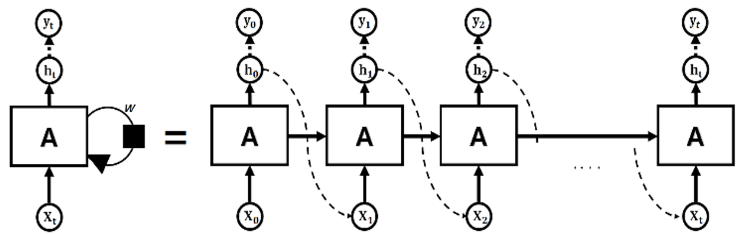
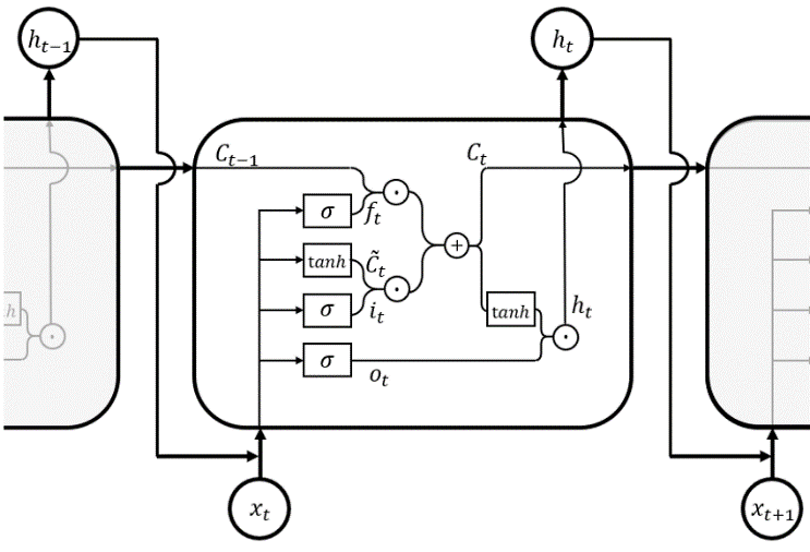
Figure 1. Structure of Recurrent Neural Network

Figure 2. Inner structure of a Long Short-Term Memory cell

Finally, the output gate decides what values are to be selected, combining $o_{t}$ with the $tanh$-applied state $C_{t}$ as output $h_{t}$. The new cell state is a combination of the forget-gate-applied former cell state $C_{t-1}$ and the new $tanh$-applied state $C_{t}$.

$o_{t}\hskip 2.84526pt=\hskip 2.84526pt\sigma(\hskip 2.84526ptW_{o}\cdot[h_{t-1},x_{t}]+b_{o}\hskip 2.84526pt)$

$C_{t}\hskip 2.84526pt=\hskip 2.84526ptf_{t}\hskip 2.84526pt\cdot\hskip 2.84526ptC_{t-1}\hskip 5.69054pt+\hskip 5.69054pti_{t}\hskip 2.84526pt\cdot\hskip 2.84526pt\tilde{C}_{t}$

$h_{t}\hskip 2.84526pt=\hskip 2.84526pto_{t}\hskip 5.69054pt\cdot\hskip 5.69054pttanh(C_{t})$

The cell state $C_{t}$ and output $h_{t}$ will be passed to the next time step, and will go through a same process. Depending on the task, further activation functions such as the Softmax or Hyperbolic tangent can be applied to $h_{t}$’s. In our paper’s case, which is a regression task that has output with values bounded between -1 and 1, we apply the hyperbolic tangent function to the output of the last element of data vector X. Figure 2 provides a visual illustration to aid understanding of the LSTM cell inner structure.

4 Research Methodology

4.1 ARIMA

4.1.1 the Data

In this paper, we resolve to utilize the ‘adjusted close’ price of the S&P500 firms . The price data from 2008-01-01 to 2017-12-31 of the S&P500 firms are downloaded. The data has a small ratio of missing values. The ratio of missing price data of each asset is around 0.1%, except for one asset with ticker ‘MMM’, which has a ratio around 1.1%. Although MMM’s ratio is not that high, missing data imputation seems improbable because the missing values are found in consecutive days, creating great chasms in the time series. This may cause distortion when computing the correlation coefficient. So we exclude MMM from our research. For other assets, we impute the missing data at time t with the value of time t-1 for all assets. Then, we randomly select 150 stocks from the fully imputed price dataset. The randomly selected 150 firms’ tickers are enlisted in ‘Appendices A’.
Using the fully imputed 150 set of price data, we compute the correlation coefficient of each pair of assets with a 100-day time window. In order to add diversity, we set five different starting values, $1^{st},21^{st},41^{st},61^{st}$ and $81^{st}$, and each apply a rolling 100-day window with a 100-day stride until the end of the dataset. This process renders 55875 sets of time series data (${}_{150}\textrm{C}_{2}\cdot 5$), each with 24 time steps. Finally, we generate the train, development, and test1&2 data set with the 55875 $\times$ 24 data. We split the data as follows by means to implement the walk-forward optimization [15] in the model evaluation phase.

$\cdot$	Train set :	index 1    ~   21
$\cdot$	Development set :	index 2    ~   22
$\cdot$	Test1 set :	index 3    ~   23
$\cdot$	Test2 set :	index 4    ~   24

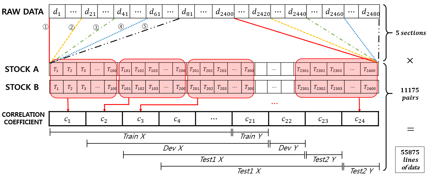
Figure 3. Data generation scheme

4.1.2 Model Fitting

Before fitting an ARIMA model, the order of the model must be specified. The ACF plot and the PACF plot aids the decision process. Most of the datasets showed an oscillatory trend that seemed close to a white noise as shown in Table 1. Other notable trends includes an increasing/decreasing trend, occasional big dips while steady correlation coefficient, and having mixed oscillatory-steady periods. Although the ACF/PACF plots indicate that a great portion of the datasets are close to a white noise, several orders (p, d, q) = (1, 1, 0), (0, 1, 1), (1, 1, 1), (2, 1, 1), (2, 1, 0) seems applicable. We fit the ARIMA model with these five orders and select the model with the least AIC value, for each train/development/test1/test2 dataset’s data. The method we use to compute the log likelihood function for the AIC metric is the maximum likelihood estimator.
After fitting the ARIMA model, we generate predictions for each 21 time steps to compute the residual value. Then, the last data point of each data will serve as the target variable Y, and the rest as variable X (Figure 3). The newly X/Y-split datasets will be the input values for the next LSTM model sector.

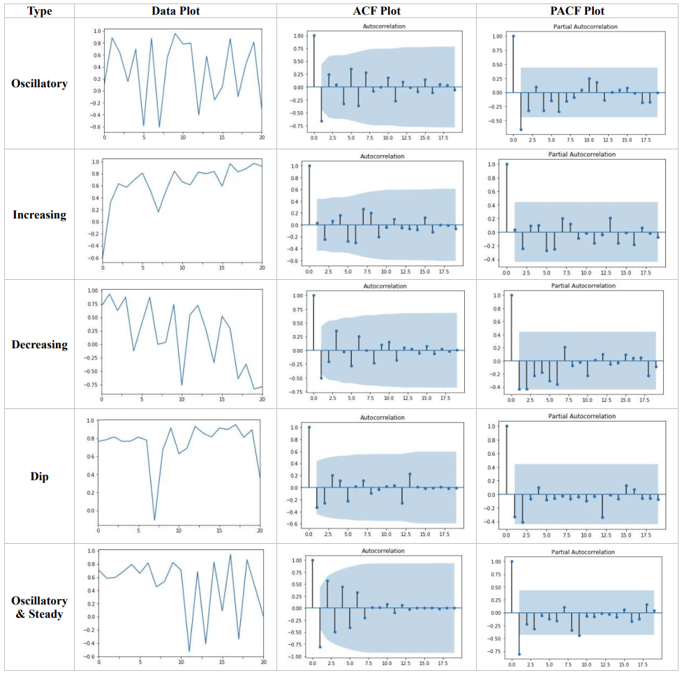
Table 1. Notable trends and the ACF/PACF of 1-level-differenced data

4.1.3 the Algorithm

Algorithm 1. ARIMA model fitting algorithm

1: datasets = [train, dev, test1, test2] 2: orders = [ (1,1,0), (0,1,1), (1,1,1), (2,1,1), (2,1,0) ] 3: for all data in datasets do 4:         X = empty list 5:         Y = empty list 6:         for all time-series T in data do 7:              models = empty list 8:              for all order in orders do 9:                   $\textit{M}_{order}=$ fit ARIMA(T, order) 10:                   add $\textit{M}_{order}$ to models 11:              with least-AIC model $\textit{M}_{\textit{fit}}$ in models 12:                   residual = X - predict(T, $\textit{M}_{\textit{fit}}$) 13:              add residual[0:20] to X 14:              add residual[20] to Y 15:         save X, Y

4.2 LSTM

4.2.1 the Data

We use the residual values, derived from the ARIMA model, of the 150 randomly selected S&P500 stocks as input for the LSTM model. The datasets include the train X/Y, development X/Y, test1 X/Y, and test2 X/Y. Each X dataset has 55875 lines with 20 time steps, with a corresponding Y dataset for each time series (Figure 3). The data points are generally around 0, as the input is a residual dataset (Figure 4).

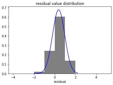
Figure 4. Data Point Distribution

4.2.2 Model Training

The architecture of the model for our task is an RNN neural network that employs 25 LSTM units. The last outputs of 25 LSTM units is merged into a single value with a fully connected layer. Then, the value will be passed through a doubled-hyperbolic tangent activation function to output a single final prediction. The doubled-hyperbolic tangent is simply the hyperbolic tangent function scaled by a factor of 2. Figure 5 shows a simplified architecture of the model.
When training the model, it is crucial to keep an eye on overfitting. Overfitting occurs when the model fits excessively on dataset while training. Hence, the predictive performance on the train dataset will be high, but will be poor on other newly introduced data. To monitor this problem, a separate set of development dataset is used. We train the LSTM model with the train dataset until the predictive performances on the train dataset and development dataset become similar to each other.
The dropout method is one of the widely used methods to prevent overfitting. It prevents the neurons to develop interdependency, which causes overfitting. This is executed by simply turning off neurons in the network during training with probability $p$. Then, in the testing phase, dropout is disabled and each weight values are multiplied by $p$, to scale down the output value into a desired boundary. Moreover, dropout has the effect of training multiple neural networks and averaging the outputs [14].
Other than dropout, we considered more regularization to prevent overfitting. There are mainly two types of regularization methods: Lasso regularization (L1) and Ridge regularization (L2). These regularizers keep the weight values of each network in the LSTM model from becoming too large. Big parameter values of each layers may cause the network to focus severely on few features, which may result in overfitting. A general expression of the error function with regularization is as follows.

$$\sum_{i=1}^{n}\{Y_{i}-(W\cdot X_{i}+b)\}^{2}+\lambda_{W}\sum_{i=1}^{k}\sum_{j=1}^{k^{\prime}}W_{ij}^{2}+\lambda_{b}\sum_{i=1}^{l}\sum_{j=1}^{l^{\prime}}b_{ij}^{2}$$

Parameters $\lambda_{\textit{W}}$ and $\lambda_{\textit{b}}$ determine the intensity of regularization of the cost function. If the lambda values are too high, the model will be under-trained. On the other hand, if they are too low, regularization affect will be minimal. In our model, after trial and error, it turned out that not applying any regularization performs better. We tried more complex architectures with regularization, but for all architectures, models with no regularization had superior outputs.
Another problem to pay attention to when training a neural network model is the vanishing/exploding gradient. This is particularly emphatic for RNN’s. Due to a deep propagation through time, the gradients far away from the output layer tend to be very small or large, preventing the model from training properly. The remedy for this problem is the LSTM cell itself. The LSTM is capable of connecting large time intervals without loss of information [16].
Other miscellaneous details about the training process includes the use of mini-batch of size 500, the ADAM optimization function et cetera. For detail, refer to the LSTM section source codes in ‘Appendices B’.

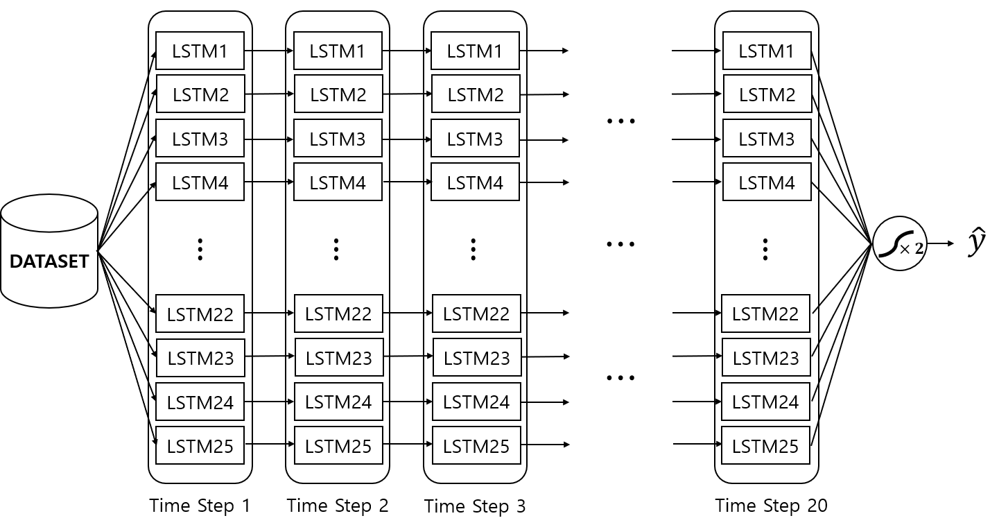
Figure 5. LSTM model sector architecture

4.2.3 Evaluation

The walk-forward optimization method [15] is used as the evaluation method. The walk-forward optimization requires that a model be fitted for each rolling time intervals. Then, for each time interval, the newly trained model is tested on the next time step. This ensures the robustness of the model fitting strategy. However, this process is computationally expensive. In addition, our paper’s motive is to fit parameters of a model that generalizes well on various assets as well as on different time periods. Thus, it is needless to train multiple models to approve of the model-fitting strategy. Rather than training a new model for each rolling train-set window, we resolve to train a single model with the first window and apply it to three time intervals – the development set and the test1/test2 set.
We selected our optimal model with the Mean Squared Error (MSE) metric. That is, the cost function of our model was the MSE. For further evaluation, the Mean Absolute Error (MAE) and Root Mean Squared Error(RMSE) was also investigated.

MSE $=\frac{\displaystyle 1}{\displaystyle n}$ $\sum_{i=1}^{n}(y_{i}-\hat{y}_{i})^{2}$

MAE $=\frac{\displaystyle 1}{\displaystyle n}$ $\sum_{i=1}^{n}|y_{i}-\hat{y}_{i}|$

The selected optimal model is then tested on two recent time periods. We use two separate datasets to test the model because the development set is deemed to be involved in the learning process as well.
If the model’s correlation coefficient prediction on two time periods turn out decent as well, we then test our model against former financial predictive models. The MSE and MAE values are computed for the four financial models as well. For the constant correlation model and the multi-group model, we regarded the 150 assets we selected randomly to be our portfolio constituents.

4.2.4 the Algorithm

Algorithm 2. LSTM model training algorithm

1: read [train_X/Y, dev_X/Y, test1_X/Y, test2_X/Y] 2: define model 3:         add LSTM(units = 25) 4:         add Dense(shape=(25,1), activation=‘double-tanh’) 5: Repeat 6:         Forward_propagate model with train_X 7:         Backward_propagate model with train_Y 8:         Update model parameters 9:         train_MSE, train_MAE = model(train_X, train_Y) 10:         dev_MSE, dev_MAE = model(dev_X, dev_Y) 11:         if train_MSE, dev_MSE converged 12:              end Repeat 13: test1_MSE, test1_MAE = model(test1_X, test1_Y) 14: test2_MSE, test2_MAE = model(test2_X, test2_Y)

5 Results And Evaluation

After around 200 epochs, the train dataset’s MSE value and development dataset’s MSE value started to converge (Figure 6). The MAE learning curve showed a similar trend as well. Among the models, we selected the $247^{th}$ epoch’s model. The epoch was decided based on both the overfitting metric and the performance metric. The overfitting metric was represented with the normalized value of the MSE difference between the train & development dataset. And the performance metric was represented with the normalized value of the MSE sum of the train & development datset. Then, the sum of the two normalized value was calculated to find the epoch that had the least value. The mathematical representation of the criterion is as follows.

$criterion=\frac{\displaystyle diff_{MSE}-mean(diff_{MSE})}{\displaystyle stdev(diff_{MSE})}+\frac{\displaystyle sum_{MSE}-mean(sum_{MSE})}{\displaystyle stdev(sum_{MSE})}$

With the selected ARIMA-LSTM hybrid model, the MSE, RMSE and MAE values of the prediction were calculated. The MSE value on the development, test1, and test2 dataset were 0.1786, 0.1889, 0.2154 each. The values have small variations, which means the model has been generalized adequately.
Then, the metric values were compared with that of other financial models. Among the financial models, the Constant Correlation model performed the best on our 150 S&P500 stocks’ dataset, just as what the empirical study of E. J. Elton et al. has shown [3]. However, its performance was nowhere near the ARIMA-LSTM hybrid model’s predictive capacity. The ARIMA-LSTM’s MSE value was nearly two thirds of that of other equivalent models. The MAE metric also showed clear outperformance. Table 2 demonstrates all metrics’ values for every dataset, for each model. The least value of each metric was boldfaced. Here, we can easily notice the how all the metric values of the ARIMA-LSTM model are in boldface.
For further investigation, we tested our final model on different assets in the S&P500 firms. Excluding the 150 assets we have already selected to train our model, we randomly selected 10 assets and generated datasets with identical structures as the ones used in the model training and testing. This generates 180 lines of data. We then pass the data into our ARIMA-LSTM hybrid model and evaluate the predictions with the MSE, RMSE and MAE metrics. We iterate this process 10 times to check for model stability. The output of 10 iterations are demonstrated in Table 3.
The MSE values of 10 iterations range from 0.1447 to 0.2353. Although there is some variation in the results compared to the Test1 & 2, this may be due to a relatively small sample size, and the outstanding performance of the model makes it negligible. Therefore, we may carefully affirm that our ARIMA-LSTM model is robust.

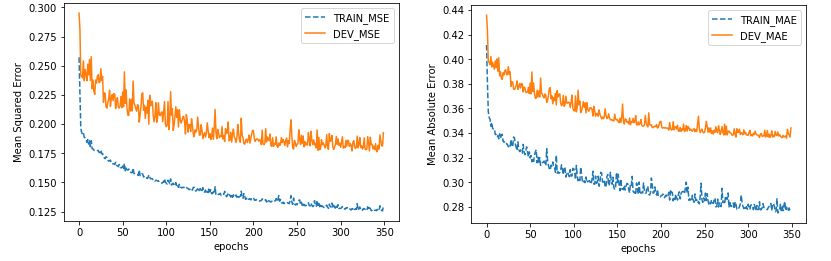
Figure 6. Learning curves of the ARIMA-LSTM model training process

Development dataset Test1 dataset Test2 dataset MSE RMSE MAE MSE RMSE MAE MSE RMSE MAE ARIMA-LSTM .1786 .4226 .3420 .1889 .4346 .3502 .2154 .4641 .3735 Full Historical .4597 .6780 .5449 .5005 .7075 .5741 .4458 .6677 .5345 Constant Correlation .2954 .5435 .4423 .2639 .5137 .4436 .2903 .5388 .4576 Single-Index .4035 .6352 .5165 .3517 .5930 .4920 .3860 .6213 .5009 Multi-Group .3079 .5549 .4515 .2910 .5394 .4555 .2874 .5361 .4480

Table 2. ARIMA-LSTM model performance results and its comparison

Iter. Tickers MSE RMSE MAE 1 PRGO, MRO, ADP, HCP, FITB, PEG, SYMC, EOG, MDT, NI .2025 .4500 .3732 2 STI, COP, MCD, AON, JBHT, DISH, GS, LRCX, CTXS, LEG .1517 .3895 .3331 3 TJX, EMN, JCI, C, BIIB, HOG, PX, PH, XEC, JEC .1680 .4099 .3476 4 ROP, AZO, URI, TROW, CMCSA, SLB, VZ, MAC, ADS, MCK .1966 .4434 .3605 5 RL, CVX, SRE, PFE, PCG, UTX, NTRS, INCY, COP, HRL .2353 .4851 .3951 6 FE, STI, EA, AAL, XOM, JNJ, COL, APC, MCD, VFC .2175 .4664 .3709 7 BBY, AXP, CAG, TGT, EMR, MNST, HSY, MCK, INCY, WBA .1447 .3804 .3094 8 BXP, HST, NI, ESS, GILD, TSN, T, MSFT, LEG, COST .1997 .4469 .3518 9 CVX, FE, WMT, IDXX, GOOGL, PKI, EQIX, DISH, FTI, HST .1785 .4225 .3331 10 NKE, VAR, DVN, VRSN, PFG, HAS, UNP, EQT, FE, AIV .2168 .4656 .3742

Table 3. ARIMA-LSTM testing results on different asset combinations

6 Conclusion

The purpose of our empirical study was to propose a model that performs superior to extant financial correlation coefficient predictive models. We adopted the ARIMA-LSTM hybrid model in an attempt to first filter out linearity in the ARIMA modeling step, then predict nonlinear tendencies in the LSTM recurrent neural network. The testing results showed that the ARIMA-LSTM hybrid model performs far superior to other equivalent financial models. Model performance was validated on both different time periods and on different combinations of assets with various metrics such as the MSE, RMSE, and the MAE. The values nearly halved that of the Constant Correlation model, which, in our experiment, turned out to perform best among the four financial models. Judging from such outperformance, we may presume that the ARIMA-LSTM hybrid model has sufficient predictive potential. Thus, the ARIMA-LSTM model as a correlation coefficient predictor for portfolio optimization would be considerable. With a better predictor, the portfolio is optimized more precisely, thereby enhancing returns in investments.
However, our experiment did not cover time periods before the year 2008. So our model may be susceptible to specific financial conditions that were not present in the years between 2008 and 2017. But financial anomalies and noises are always prevalent. It is impossible to embrace all probable specific tendencies into the model. Hence, further research into dealing with financial black swans is called for.

Appendix A 150 S&P500 Stocks

* This is the list of tickers of the 150 randomly selected S&P500 stocks.

CELG	PXD	WAT	LH	AMGN	AOS
EFX	CRM	NEM	JNPR	LB	CTAS
MAT	MDLZ	VLO	APH	ADM	MLM
BK	NOV	BDX	RRC	IVZ	ED
SBUX	GRMN	CI	ZION	COO	TIF
RHT	FDX	LLL	GLW	GPN	IPGP
GPC	HPQ	ADI	AMG	MTB	YUM
SYK	KMX	AME	AAP	DAL	A
MON	BRK	BMY	KMB	JPM	CCI
AET	DLTR	MGM	FL	HD	CLX
OKE	UPS	WMB	IFF	CMS	ARNC
VIAB	MMC	REG	ES	ITW	NDAQ
AIZ	VRTX	CTL	QCOM	MSI	NKTR
AMAT	BWA	ESRX	TXT	EXR	VNO
BBT	WDC	UAL	PVH	NOC	PCAR
NSC	UAA	FFIV	PHM	LUV	HUM
SPG	SJM	ABT	CMG	ALK	ULTA
TMK	TAP	SCG	CAT	TMO	AES
MRK	RMD	MKC	WU	CAN	HIG
TEL	DE	ATVI	O	UNM	VMC
ETFC	CMA	NRG	RHI	RE	FMC
MU	CB	LNT	GE	CBS	ALGN
SNA	LLY	LEN	MAA	OMC	F
APA	CDNS	SLG	HP	XLNX	SHW
AFL	STT	PAYX	AIG	FOX	MA

Appendix B LSTM Model Source Code

* This source code is a simplified version; unnecessary portions were contracted or omitted. For original and other relevant source codes, visit
‘https://github.com/imhgchoi/Corr_Prediction_ARIMA_LSTM_Hybrid’.

⬇

import pandas as pd

import numpy as np

import os

from keras.models import Sequential, load_model

from keras.layers import Dense, LSTM, Activation

from keras import backend as K

from keras.utils.generic_utils import get_custom_objects

from keras.callbacks import ModelCheckpoint

from keras.regularizers import l1_l2

# Train - Dev - Test Generation

train_X= pd.read_csv(’~/train_dev_test/after_arima/train_X.csv’)

dev_X = pd.read_csv(’~/train_dev_test/after_arima/dev_X.csv’)

test1_X = pd.read_csv(’~/train_dev_test/after_arima/test1_X.csv’)

test2_X = pd.read_csv(’~/train_dev_test/after_arima/test2_X.csv’)

train_Y = pd.read_csv(’~/train_dev_test/after_arima/train_Y.csv’)

dev_Y = pd.read_csv(’~/train_dev_test/after_arima/dev_Y.csv’)

test1_Y = pd.read_csv(’~/train_dev_test/after_arima/test1_Y.csv’)

test2_Y = pd.read_csv(’~/train_dev_test/after_arima/test2_Y.csv’)

# data sampling

STEP = 20

_train_X = np.asarray(train_X).reshape((int(1117500/STEP), 20, 1))

_dev_X = np.asarray(dev_X).reshape((int(1117500/STEP), 20, 1))

_test1_X = np.asarray(test1_X).reshape((int(1117500/STEP), 20, 1))

_test2_X = np.asarray(test2_X).reshape((int(1117500/STEP), 20, 1))

_train_Y = np.asarray(train_Y).reshape(int(1117500/STEP), 1)

_dev_Y = np.asarray(dev_Y).reshape(int(1117500/STEP), 1)

_test1_Y = np.asarray(test1_Y).reshape(int(1117500/STEP), 1)

_test2_Y = np.asarray(test2_Y).reshape(int(1117500/STEP), 1)

#define custom activation

class Double_Tanh(Activation):

def __init__(self, activation, **kwargs):

super(Double_Tanh, self).__init__(activation, **kwargs)

self.__name__ = ’double_tanh’

def double_tanh(x):

return (K.tanh(x) * 2)

get_custom_objects().update({’double_tanh’:Double_Tanh(double_tanh)})

# Model Generation

model = Sequential()

model.add(LSTM(25, input_shape=(20,1)))

model.add(Dense(1))

model.add(Activation(double_tanh))

model.compile(loss=’mean_squared_error’, optimizer=’adam’, metrics=[’mse’, ’mae’])

# Fitting the Model

model_scores = {}

epoch_num=1

for _ in range(50):

# train the model

dir = ’~/models/hybrid_LSTM’

file_list = os.listdir(dir)

if len(file_list) != 0 :

epoch_num = len(file_list) + 1

recent_model_name = ’epoch’+str(epoch_num-1)+’.h5’

filepath = ’~/models/hybrid_LSTM/’+recent_model_name

model = load_model(filepath)

filepath = ’~/models/hybrid_LSTM/epoch’+str(epoch_num)+’.h5’

checkpoint = ModelCheckpoint(filepath, monitor=’loss’, verbose=1, save_best_only=False, mode=’min’)

callbacks_list = [checkpoint]

if len(callbacks_list) == 0:

model.fit(_train_X, _train_Y, epochs=1, batch_size=500, shuffle=True)

else:

model.fit(_train_X, _train_Y, epochs=1, batch_size=500, shuffle=True, callbacks=callbacks_list)

# test the model

score_train = model.evaluate(_train_X, _train_Y)

score_dev = model.evaluate(_dev_X, _dev_Y)

# get former score data

df = pd.read_csv(’~/models/hybrid_LSTM.csv’)

train_mse = list(df[’TRAIN_MSE’])

dev_mse = list(df[’DEV_MSE’])

train_mae = list(df[’TRAIN_MAE’])

dev_mae = list(df[’DEV_MAE’])

# append new data

train_mse.append(score_train[1])

dev_mse.append(score_dev[1])

train_mae.append(score_train[2])

dev_mae.append(score_dev[2])

# organize newly created score dataset

model_scores[’TRAIN_MSE’] = train_mse

model_scores[’DEV_MSE’] = dev_mse

model_scores[’TRAIN_MAE’] = train_mae

model_scores[’DEV_MAE’] = dev_mae

# save newly created score dataset

model_scores_df = pd.DataFrame(model_scores)

model_scores_df.to_csv(’~/models/hybrid_LSTM.csv’)

References

- [1] G. Francis A. N. Refenes, A. Zapranis. Stock performance modeling using neural networks: A comparative study with regression models. Neural Networks, 7(2):375–388, 1994.
- [2] R.A. de Oliveira D.M.Q. Nelson, A.C.M. Pereira. Stock market’s price movement prediction with lstm neural networks. In 2017 International Joint Conference on Neural Networks (IJCNN), pages 1419–1426, 2017.
- [3] T. J. Urich E. J. Elton, M. J. Gruber. Are betas best? Journal of Finance, 33:1375–1384, 1978.
- [4] M. J. Gruber E.J. Elton. Modern portfolio theory, 1950 to date. Journal of banking And Finance, 21:1743–1759, 1997.
- [5] M. W. Padberg E.J. Elton, M. J. Gruber. Simple rules for optimal portfolio selection: The multi group case. Journal of Financial and Quantitative Analysis, 12(3):329–349, 1977.
- [6] E. Jondeau F. Chesnay. Does correlation between stock returns really increase during turbulent periods? Economic Notes, Vol.30, no.1-2001:53–80, 2001.
- [7] H. M. Markowitz F. J. Fabozzi, F. Gupta. The legacy of modern portfolio theory. The Journal of Investing, Vol. 11, No. 3:7–22, 2002 Fall.
- [8] F. Cummins F.A. Gers, J. Schmidhuber. Learning to forget: Continual prediction with lstm. Technical Report, IDSIA-01-99, 1999.
- [9] G. Jenkins G.E.P. Box. Time series analysis, forecasting and control. Holden-Day, San Francisco, CA, 1970.
- [10] R. D. Nelson J.V. Hansen. Time-series analysis with neural networks and arima-neural network hybrids. Journal of Experimental And Theoretical Artificial Intelligence, 15:3:315–330, 2003.
- [11] T. Tanigawa K. Kamijo. Stock price pattern recognition - a recurrent neural network approach. 1990 IJCNN International Joint Conference on Neural Networks, vol.1, San Diego, CA, USA:215–221, 1990.
- [12] J. H. Bang M. Dixon, D. Klabjan. Classification-based financial markets prediction using deep neural networks. Algorithmic Finance, 6(3-4):67–77, 2017.
- [13] H. M. Markowitz. Portfolio selection. The Journal of Finance, Vol.7, No.1:77–91, Mar. 1952.
- [14] A. Krizhvsky I. Sutskever R. Salakhutdinov N. Srivastave, G. Hinton. Dropout: A simple way to prevent neural networks from overfitting. Journal of Machine Learning Research, 15:1929–1958, 2014.
- [15] P. Grzegorzewski P. ladyzynski, K. Zbikowski. Stock trading with random forests, trend detection tests and force index volume indicators. Artificial Intelligence and Soft Computing, Lecture Notes in Computer Science, 7895:pp.441–452, 2013.
- [16] J. Schmidhuber S. Hochreiter. Long short-term memory. Neural Computation, 9(8):1735–1780, 1997.
- [17] W.F. Sharpe. A simplified model for portfolio analysis. Management Science, 13:277–293, 1963.
- [18] G. Swales Y. Yoon. Predicting stock price performance: A neural network approach. System Sciences, Proceedings of the Twenty-Fourth Annual Hawaii International Conference on, Vol. 4, IEEE:156–162, 1991.
- [19] G.P. Zhang. Time series forecasting using a hybrid arima and neural network model. Neurocomputing, 50:159–175, 2003.
- [20] F. Zhao. Forecast correlation coefficient matrix of stock returns in portfolio analysis, 2013.