Designing Adaptive Neural Networks
for Energy-Constrained Image Classification

Abstract.

As convolutional neural networks (CNNs) enable state-of-the-art computer vision applications, their high energy consumption has emerged as a key impediment to their deployment on embedded and mobile devices. Towards efficient image classification under hardware constraints, prior work has proposed adaptive CNNs, i.e., systems of networks with different accuracy and computation characteristics, where a selection scheme adaptively selects the network to be evaluated for each input image. While previous efforts have investigated different network selection schemes, we find that they do not necessarily result in energy savings when deployed on mobile systems. The key limitation of existing methods is that they learn only how data should be processed among the CNNs and not the network architectures, with each network being treated as a blackbox.

To address this limitation, we pursue a more powerful design paradigm where the architecture settings of the CNNs are treated as hyper-parameters to be globally optimized. We cast the design of adaptive CNNs as a hyper-parameter optimization problem with respect to energy, accuracy, and communication constraints imposed by the mobile device. To efficiently solve this problem, we adapt Bayesian optimization to the properties of the design space, reaching near-optimal configurations in few tens of function evaluations. Our method reduces the energy consumed for image classification on a mobile device by up to $6\times$, compared to the best previously published work that uses CNNs as blackboxes. Finally, we evaluate two image classification practices, i.e., classifying all images locally versus over the cloud under energy and communication constraints.

1. Introduction

Deep convolutional neural networks (CNNs) have been established as one of the most powerful machine learning techniques for a plethora of computer vision applications. In response to the growing demand for state-of-the-art performance in real-world deployment, the complexity of CNNs has increased significantly, which has come at the significant cost of energy consumption. As a consequence, the energy requirements of CNNs have emerged as a key impediment preventing their deployment on energy-constrained embedded and mobile devices, such as Internet-of-Things (IoT) nodes, wearables, and smartphones. For instance, object classification with AlexNet can drain the smartphone battery within an hour (Yang et al., 2017). This design challenge has resulted in an ever-increasing interest to develop energy-efficient image classification solutions (Russakovsky et al., 2015).

As means to reducing the average classification cost by trading off the accuracy, prior art has investigated the use of adaptive CNNs, i.e., systems of CNNs with different accuracy and computation characteristics, where a selection scheme adaptively selects the network to be evaluated for each input image (Bolukbasi et al., 2017). A large body of work from both industry (Goodfellow et al., 2013) and academia (Venkataramani et al., 2015; Panda et al., 2016, 2017a; Park et al., 2015; Panda et al., 2017b) exploits the insight that a large portion of an image dataset can be correctly classified by simpler CNN architectures. Nevertheless, all previous approaches focus only on learning how data should be processed among the CNNs and not the network architectures. Hence, existing adaptive CNNs are optimized only with respect to the network selection scheme, with each CNN being treated as a blackbox (i.e., pre-trained off-the-shelf CNN).

Moreover, prior work has not explicitly profiled energy savings on state-of-the-art mobile systems on chip (SoCs). Thus, the reported savings could be attributed to either significant runtime reduction when executing smaller CNNs on powerful workstation GPUs or to gate count (area, ergo power) reduction on ASIC-like designs. In our analysis, however, we found that the energy-limited mobile SoCs have small headroom for savings, hence limiting the overall effectiveness of existing adaptive CNN designs. For example, our results show that existing methods, if tested on commercial Nvidia Tegra TX1 platforms, could actually lead to an increase in energy consumption under strict accuracy constraints.

In this paper, we make the following observation: the minimum energy achieved by adaptive CNNs can be significantly reduced if the architecture of each individual network is optimized jointly with the network selection scheme. Our key insight is to treat the architectural choices of each network (e.g., number of hidden units, number of feature maps, etc.) as hyper-parameters. To the best of our knowledge, there is no global, systematic methodology for the hardware-constrained hyper-parameter optimization of adaptive CNNs based on hardware measurements on a real mobile platform, even though prior art has highlighted this suboptimality (Park et al., 2015). Such observation constitutes the key motivation behind our work.

Our work makes the following contributions:

1. Globally optimized adaptive CNNs: To the best of our knowledge, we are first to optimize systems of adaptive CNNs for both the network architectures and the network selection scheme, under hardware constraints imposed by the mobile platforms. Our methodology identifies designs that outperform the best previously published approaches in resource-constrained adaptive CNNs by up to $6\times$ in terms of minimum energy per image and by up to $31.13\%$ in terms of accuracy improvement, when tested on a commercial Nvidia mobile SoC and the CIFAR-10 dataset.

2. Adaptive CNNs as hyper-parameter problem: To enable this design paradigm, our work formulates the design of adaptive CNNs as a hyper-parameter optimization problem, where the architectural parameters of each network, such as the number of hidden units and the number of feature maps, are treated as hyper-parameters to be jointly optimized intrinsically with respect to hardware constraints. We show that our formulation is generic and able to incorporate different design goals that are significant in a mobile design space. In our results, we consider optimization under energy, accuracy, and communication constraints.

3. Enhancing Bayesian optimization for designing adaptive CNNs: To solve this challenging hyper-parameter optimization problem, we adapt Bayesian optimization (BO) to exploit properties of the mobile design space. In particular, we observe that once the accuracy and hardware measurements (power, runtime, energy) have been obtained for a set of candidate CNN designs, it is relatively inexpensive to sweep over different network selection schemes to populate the optimization process with more data points. This fine-tuning step allows the modified BO, which we denote as $BO^{+}$ in the remainder of the paper, to reach the near-optimal region faster compared to a hardware-unaware BO methodology, and to effectively reach the optimal designs identified by exhaustive (grid) search.

4. Insightful design space exploration: Image classification under mobile hardware constraints constitutes a challenging design space with several trade-offs possible. We exploit the effectiveness of our method as a useful aid for design space exploration, and we evaluate two representative practices for image classification with adaptive CNNs, i.e., classifying all images locally or over the cloud under energy and communication constraints. We investigate both these methods under different energy, communication, and accuracy constraints on a commercial Nvidia system, thus providing computer vision practitioners and mobile platform designers with insightful directions for future research.

2. Related Work

Adaptive CNN execution: Prior art has shown that a large percentage of images in an image dataset are easy to classify even with a simpler CNN configuration (Venkataramani et al., 2015). Since the “easy” examples do not require the computational complexity and overhead of a massive, monolithic CNN, this inspires the use of adaptive CNNs with varying levels of accuracy and complexity. This insight of dynamically trading off accuracy with energy-efficiency can be found in several existing approaches from different groups and under different names (e.g., conditional (Panda et al., 2016), scalable (Venkataramani et al., 2015), etc.).

The early efforts to enable energy efficiency were based on “early-exit” conditions placed at each layer of a CNN, aiming at bypassing later stages of a CNN if the classifier has a “confident” prediction in earlier stages. These methods include the scalable-effort classifier (Venkataramani et al., 2015), the conditional deep learning classifier (Panda et al., 2016), the distributed neural network (Teerapittayanon et al., 2017), the edge-host partitioned neural network (Ko et al., 2018), and the cascading neural network (Leroux et al., 2017). However, recent work shows that adaptive execution at the network level outperforms layer-level execution (Bolukbasi et al., 2017). Hence, we focus on network-level designs. We note that our formulation is generic and can be flexibly applied to the layer-wise case.

At the network-level, Takhirov et al. have trained an adaptive classifier (Takhirov et al., 2016). However, the method is applied on regression-based classifiers of low complexity. Park et al. propose a two-network adaptive design (Park et al., 2015), where the decision of which network to process the input data is done by looking into the “confidence score” of the network output. Bolukbasi et al. extend the formulation of network-level adaptive systems to multiple networks (Bolukbasi et al., 2017). Finally, other works extend the cascading execution to more tree-like structures for image classification (Panda et al., 2017a; Roy et al., 2018).

Nevertheless, existing approaches rely on off-the-shelf network architectures without studying their architectures jointly. While prior art has explicitly highlighted this limitation (Park et al., 2015), to the best of our knowledge there is no global, systematic methodology for the hardware-constrained hyper-parameter optimization of adaptive CNNs. On the contrary, our work is the first to cast this problem as a hyper-parameter optimization problem and to enhance a BO methodology to efficiently solve it, thus effectively designing both the CNN architectures and the chooser functions among them.

Pruning- and quantization-based energy efficient CNNs: Beyond adaptive CNNs, there are two key approaches that address energy efficiency based on CNN parameter reduction. First, prior art has investigated pruning-based methods to reduce the network connections (Han et al., 2015; Dai et al., 2017; Yang et al., 2017). Second, other works reduce directly the computational complexity of CNNs by quantizing the network weights (Ding et al., 2018). Nevertheless, recent work argues that the effectiveness of methods targeting the weights and parameters of a monolithic CNN relies heavily on the performance of this baseline (seed) network (Gordon et al., 2018). Hence, in our case we focus on adaptive CNN structures to globally optimize and identify the sizing of the different CNNs. Existing approaches are complimentary and could be used to further reduce computational cost given the globally optimal “seed” identified with our approach.

Hyper-parameter optimization: Hyper-parameter optimization of CNNs has emerged as an increasingly challenging and expensive process, dubbed by many researchers to be more of an art than science. In the context of hardware-constrained optimization, among different model-based methods for hyper-parameter optimization, several groups have shown that BO is effective for architectural search in CNNs (Snoek et al., 2012) and has been successfully used for the co-design of hardware accelerators and NNs (Hernández-Lobato et al., 2016b; Reagen et al., 2017), of NNs under runtime (Hernández-Lobato et al., 2016a) and power constraints (Stamoulis et al., 2018). Nevertheless, BO has not been considered in the design space of adaptive CNNs. We employ BO to identify both the flow of input images among the CNNs and their sizing (e.g., number of filters, kernel sizes, etc.).

It is worth noting that existing methodologies rely on simplistic proxies of the hardware performance (e.g., counts of the NN’s weights (Gelbart et al., 2014) or energy per operation assumptions (Smithson et al., 2016; Rouhani et al., 2016)), or simulation results (Reagen et al., 2017). Since our target application is the mobile and embedded design space, we employ BO with all network architectures sampled and optimized for on commercial mobile platforms (i.e., NVIDIA boards) based on actual hardware measurements. In addition, our work is the first to consider BO under constraints for both the communication and computation energy consumption.

3. Background

3.1. Adaptive Neural Networks

Image classification in an adaptive CNN is intuitive. To allow for inference efficiency, an adaptive CNN system leverages the fact that many examples are correctly classified by relatively smaller (computationally more efficient) networks, while only a small fraction of examples require larger (computationally expensive) networks to be correctly classified.

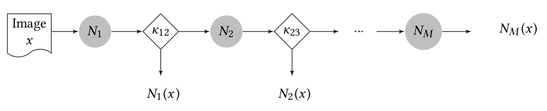
Figure 1. Classifying an image $x$ using adaptive neural networks comprised of $M$ CNNs. The system evaluates $N_{i}$ first, and based on a decision function $\kappa_{i,i+1}$ decides to use $N_{i}(x)$ as the final prediction or to evaluate networks in later stages.

Let us consider the case with $M$ neural networks to choose from, i.e. $N_{1},...,N_{i},...,N_{M}$, as shown in Figure 1. For an input data item $x\in\mathcal{X}$, we denote the predictions of each $i$-th network as $N_{i}(x)~{}\in~{}R^{K}$, which represents the probabilities of input $x$ belonging to each of the $K$ classes. Note that $K$ is the number of classes in the classification problem. To quantify the performance with respect to the classification task, we denote the loss $L(\tilde{y}(x),y)$, where $\tilde{y}(x)$ and $y\in\{1,2,~{}\dots,K\}$ are the predicted and true labels, respectively. As common practice, $\tilde{y_{i}}(x)$ is defined as the most probable class based on the current prediction, i.e., $\tilde{y_{i}}(x)=~{}$ argmax $N_{i}(x)$. To simplify notation, as loss we use the 0-1 loss $L(\tilde{y}_{i}(x),y)=\mathbbm{1}_{\tilde{y}_{i}(x)\neq y}$, showing whether the label $\tilde{y}_{i}(x)$ predicted from $N_{i}$ fails to match the true label $y$. Let $L(\tilde{y}_{i}(x),y)=L_{i}$ be the loss per network $N_{i}$. In addition, let us denote the performance (cost) term that we want to optimize for as $C_{i}=C(N_{i}(x))$ of the $i$-th network.

Given an image to be classified, the $N_{1}$ is always executed first. Next, a decision function $\kappa$ is evaluated to determine whether the classification decision from $N_{1}$ should be returned as the final answer or the next network $N_{2}$ should be evaluated. In general, we denote decision function $\kappa_{ij}:N_{i}(x)\to\{0,1\}$ that provides “confidence feedback” and decides between exiting at state $N_{i}$ (i.e., $\kappa_{ij}=0$) or continuing at subsequent stage $N_{j}$ (i.e., $\kappa_{ij}=1$).

3.2. Network selection problem

Adaptive CNNs can be seen as an optimization problem (Bolukbasi et al., 2017; Park et al., 2015). The goal of the network selection problem is to select functions $\kappa$ that optimize for the per-image inference cost (e.g., average per image runtime) subject to a constraint on the overall accuracy degradation. For the sake of notation simplicity, we write the optimization formulation for the two-network case, but the notation can be extended to an arbitrary number of networks $M$ (Bolukbasi et al., 2017):

(1) $$\begin{split}\underset{\theta_{12}}{\min}\text{~{}~{}}\mathbb{E}_{x\sim\mathcal{X}}\big{[}C_{2}\cdot\kappa_{12}\big{(}N_{1}(x)|&\theta_{12}\big{)}+C_{1}\big{]}\\ s.t.\text{~{}~{}}\mathbb{E}_{(x,y)\sim\mathcal{X}\times\mathcal{Y}}\Big{[}\Big{(}1-\kappa_{12}\big{(}N_{1}(x)|\theta_{12}\big{)}\Big{)}\cdot&\Big{(}L_{1}\big{(}\tilde{y}_{1}(x),y\big{)}-\\ &L_{2}\big{(}\tilde{y}_{2}(x),y\big{)}\Big{)}\Big{]}\leq B\end{split}$$

where the constraint here intuitively specifies that whenever the image stays at $N_{1}$, the error rate difference should not be greater than $B$. We observe that in Equation 1 the cost function is optimized only over the parameters of the decision functions, and not with respect to the parameters of the individual networks.

Selecting the decision function $\kappa$: An effective choice for the $\kappa_{ij}$ function is a threshold-based formulation (Park et al., 2015; Takhirov et al., 2016), where we define as score margin $SM$ the distance between the largest and the second largest value of the vector $N_{i}(x)=(N_{i}^{1}(x),N_{i}^{2}(x),...,N_{i}^{K}(x))$ at the output of network $N_{i}$. Intuitively, the more “confident” the CNN is about its prediction, the larger the value of the predicted output, thus the larger the value of $SM$ (since $N_{i}(x)$’s sum to 1).

Without loss of generality, in Figure 1 we show decisions between two subsequent stages, i.e., $j=i+1$, for visualization and notation simplicity. However, $N_{j}$ could be any other network in the design, i.e., $j\in M\wedge i\neq j$, hence “cascading” the execution to any later stage. For the case of $j=i+1$, let’s denote $\theta_{i,i+1}$ the threshold value for the decision function $\kappa_{i,i+1}$ between a network $N_{i}$ and a network $N_{i+1}$. If $SM$ in the output of $N_{i}$ is larger than $\theta_{i,i+1}$, the inference result from $N_{i}$ is considered correct, otherwise $N_{i+1}$ is evaluated next, i.e., $\kappa_{i,i+1}(N_{i}(x)|\theta_{i,i+1})=\mathbbm{1}_{[SM_{i}\geq\theta_{i,i+1}]}$

3.3. Network design problem

Existing methodologies have investigated the design of a monolithic CNN as a hyper-parameter optimization problem (Hernández-Lobato et al., 2016a; Stamoulis et al., 2018), where CNN architecture choices (e.g., number of feature maps per convolution layer, number of neurons in fully connected layers, etc.) are optimally selected such that the inference cost of the CNN is minimized subject to maximum error constraint $b$.

To this end, we define design space $\mathcal{H}$ of a CNN, wherein a point $h_{i}=(h_{i,1},h_{i,2},h_{i,3},...)\in\mathcal{H}$ is the vector with elements the hyper-parameters of the neural network. Intuitively, the choice of different $h$ values, i.e., of a different network architecture, results in different characteristics in both loss $L(\tilde{y}(x|h),y)$ and computational efficiency $C(N(x|h))$ of the network. For a single network, the hyper-parameter optimization problem is written:

(2) $$\begin{split}&\underset{h\in\mathcal{H}}{\min}\text{~{}~{}}\mathbb{E}_{x\sim\mathcal{X}}\big{[}C\big{(}N(x|h)\big{)}\big{]}\text{~{}~{}~{}~{}~{}~{}~{}~{}}s.t.\text{~{}~{}~{}~{}~{}~{}~{}~{}}\mathbb{E}_{(x,y)\sim\mathcal{X}\times\mathcal{Y}}\big{[}L\big{(}\tilde{y}(x|h),y\big{)}\big{]}\leq b\end{split}$$

We note that formulations based on Equation 2 do not incorporate design choices encountered in adaptive CNNs.

3.4. Key insight behind our work

In summary, the two aforementioned optimization problems are decoupled and have not been jointly studied to date. On the one hand, the network selection problem (Equation 1) assumes the architectures of CNNs (i.e., vectors $h$) to be fixed and that the networks are already available and pretrained. Consequently, the optimization problem in Equation 1 is solved only over possible $\kappa$’s. On the other hand, the network design problem (Equation 2) assumes a single monolithic CNN and cannot be directly applied to adaptive CNNs. In the following section, we describe how our methodology elegantly formulates and optimizes both problems jointly.

4. Proposed Methodology

4.1. Hyper-parameter optimization

We formulate the design of adaptive CNNs as a hyper-parameter optimization problem with respect to both the decision functions as well as the networks’ sizing. For the system of $M$ neural networks we can define design space $\mathcal{Z}$ that consists of the set of hyper-parameters for each network $h_{i}$ and hyper-parameters $\theta$’s of the decision functions $\kappa$’s, i.e., $z=(h_{1},...,h_{M},\theta_{12},\theta_{23},...),z\in\mathcal{Z}$.

Energy minimization: Our goal is to minimize the average (expected) energy consumption per image subject to a maximum accuracy degradation. Let us denote as $E(N_{i}(x|h_{i}))$ the energy consumed when executing neural network $N_{i}$ to classify an input image $x\in\mathcal{X}$. For the two-network system (i.e., $M=2$), we write:

(3) $$\begin{split}\underset{z=(h_{1},h_{2},\theta_{12})}{\min}\text{~{}~{}}\mathbb{E}_{x\sim\mathcal{X}}\Big{[}E_{2}\big{(}N_{2}(x|h_{2})\big{)}\cdot\kappa_{12}\big{(}&N_{1}(x|h_{1})|\theta_{12}\big{)}+\\ &E_{1}\big{(}N_{1}(x|h_{1})\big{)}\Big{]}\\ s.t.\text{~{}~{}}\mathbb{E}_{(x,y)\sim\mathcal{X}\times\mathcal{Y}}\Big{[}\Big{(}1-\kappa_{12}\big{(}N_{1}(x|h_{1})|&\theta_{12}\big{)}\Big{)}\cdot\\ \Big{(}L_{1}\big{(}\tilde{y}_{1}(x|h_{1}),y\big{)}-L_{2}&\big{(}\tilde{y}_{2}(x|h_{2}),y\big{)}\Big{)}\Big{]}\leq B\end{split}$$

As a key contribution of our work, note that in the proposed formulation (Equation 3) the overall energy and accuracy explicitly depend on the architecture of the networks based on the values of the respective hyper-parameters $h_{i}$. Moreover, please note that, unlike prior art that resorts in exhaustive (offline) or iterative (online) methods to find a value for the threshold (Park et al., 2015; Takhirov et al., 2016), a hyper-optimization treatment allows us to directly incorporate the $\theta$ values as hyper-parameters that will be co-optimized alongside the sizing of the networks.

Considering different design paradigms: Existing methodologies from several groups consider cases that either (i) all networks execute locally on the same hardware platform (Park et al., 2015; Takhirov et al., 2016), and (ii) some of the networks are executed on remote servers, hence some of the images will be communicated over the web (Leroux et al., 2017). The formulation of the objective function in Equation 3 allows us to consider energy consumption under different design paradigms.

First, let us consider the case where all networks are executed locally. We denote as $\tau(N_{i}(x))$ and $P(N_{i}(x))$ the runtime and power required when evaluating a neural network $N_{i}$ an input image $x\in\mathcal{X}$. The expected (per image) energy is therefore written as:

(4) $$\begin{split}\mathbb{E}_{x\sim\mathcal{X}}\Big{[}P_{2}\big{(}N_{2}(x|&h_{2})\big{)}\cdot\tau\big{(}N_{2}(x|h_{2})\big{)}\cdot\kappa_{12}\big{(}N_{1}(x|h_{1})|\theta_{12}\big{)}\\ &+P_{1}\big{(}N_{1}(x|h_{1})\big{)}\cdot\tau\big{(}N_{1}(x|h_{1})\big{)}\Big{]}\end{split}$$

Second, we consider the case where some of the images $x\in\mathcal{X}$ are sent to the server over the network and the result is being communicated back. In this case, the energy consumed is the product of the power consumed from the client node $P(N_{i}(x))$ and total runtime $\tau(N_{i}(x))$ that takes to send the image and receive the result. For the case of the two-network system, this design will correspond to having $N_{1}$ executing on the edge device and $N_{2}$ on the server machine. Hence, the total energy consumption is:

(5) $$\begin{split}&\mathbb{E}_{x\sim\mathcal{X}}\Big{[}P_{idle}\cdot\Big{(}\tau_{server}\big{(}N_{2}(x|h_{2})\big{)}+\tau_{communication}\Big{)}\cdot\\ &\kappa_{12}\big{(}N_{1}(x|h_{1})|\theta_{12}\big{)}+P_{1}\big{(}N_{1}(x|h_{1})\big{)}\cdot\tau_{edge}\big{(}N_{1}(x|h_{1})\big{)}\Big{]}\end{split}$$

where $\tau_{edge}$ and $\tau_{server}$ is the runtime when executing on the edge device and the server, respectively, and $P_{idle}$ is the idle power of the edge device while waiting for the result.

Energy-constrained optimization: We can also consider the problem of minimizing classification error, while not exceeding a maximum energy per image $E_{max}$. This design case is significant for image classification under the energy budget imposed by mobile hardware engineers. Formally, we can solve:

(6) $$\begin{split}\underset{z=(h_{1},h_{2},\theta_{12})}{\min}\text{~{}~{}}\mathbb{E}_{(x,y)\sim\mathcal{X}\times\mathcal{Y}}\Big{[}\Big{(}1-\kappa_{12}(N_{1}(x|h_{1})|&\theta_{12})\Big{)}\cdot\\ \Big{(}L_{1}\big{(}\tilde{y}_{1}(x|h_{1}),y\big{)}-L_{2}\big{(}&\tilde{y}_{2}(x|h_{2}),y\big{)}\Big{)}\Big{]}\\ s.t.\text{~{}~{}}\mathbb{E}_{x\sim\mathcal{X}}\big{[}E_{2}\big{(}N_{2}(x|h_{2})\big{)}\cdot\kappa_{12}\big{(}N_{1}(x|h_{1})|\theta_{12}\big{)}&+\\ E_{1}\big{(}N_{1}(x|&h_{1})\big{)}\big{]}\leq E_{max}\end{split}$$

4.2. Adapting Bayesian optimization

Solving Equations 3 and 6 gives rise to a daunting optimization problem, due to the fact that the constraint and objective have terms that are costly to evaluate. That is, to obtain the overall accuracy, all networks need to be trained, hence each step of an optimization algorithm can take hours to complete.

Algorithm 1 Bayesian optimization framework

1:Obj. function $f(z)$, constraint $g(z)$, constraint value $c$, design space $\mathcal{Z}$, Num. iterations $D$

2:Optimizer $z^{*}$ of adaptive neural networks

3:for $d=1,2,...,D$ do

4:     $\mathcal{M}\leftarrow$ fit models on data so far $\mathcal{D}$

5:     $z_{d}\leftarrow\operatorname*{arg\,max}_{z\in\mathcal{Z}}\alpha(z,\mathcal{M})$   // acquisition function max.

6:     // Training and profiling each network $N_{i}$

7:     for $i=1,2,...,M$ do

8:         $L_{i}(z_{i,d})\leftarrow$ train network $N_{i}$

9:         // power, runtime measurements on device

10:         $E_{i}(z_{i}^{d})\leftarrow$energy of $N_{i}$

11:     end for

12:     // Evaluate accuracy and energy consumption

13:     $u^{d},v^{d}\leftarrow$ evaluate obj. $f(z^{d})$ and const. $g(z^{d})$

14:     $\mathcal{D}=\mathcal{D}\cap\{z^{d},u^{d},v^{d}\}$

15:     // $\kappa$ function fine-tuning

16:     for each decision function $\kappa_{i,i+1}$ do

17:         for $\theta_{i,i+1}^{\prime}=0.0,...,1.0$ do

18:              $z^{d}\leftarrow(h^{d}_{1},...,h^{d}_{M},...,\theta_{ij}^{\prime},...)$

19:              $u^{\prime},v^{\prime}\leftarrow$ evaluate $f(z^{\prime})$ and $g(z^{\prime})$

20:              $\mathcal{D}=\mathcal{D}\cap\{z^{\prime},u^{\prime},v^{\prime}\}$

21:         end for

22:     end for

23:end for

24:return $z^{*}\leftarrow\operatorname*{arg\,max}_{z}\{u^{1},...,u^{D}\}\text{~{}}s.t.\text{~{}}v^{*}\leq c$

To enable energy-aware hyper-parameter optimization, we use Bayesian optimization. The effectiveness of Bayesian optimization comes from of the approximation the costly “black-box” functions with a surrogate model, based on Gaussian processes (Snoek et al., 2012), which is cheaper to evaluate. The design of adaptive CNNs (Equations 3, 6) corresponds to constrained minimizing function $f(z)$ over design space $\mathcal{Z}$ and constraint $g(z)$, i.e., ${\min}_{{z\in\mathcal{Z}}}~{}f(z)$, subject to $g(z)\leq c$. We adapt Bayesian optimization in this design space and we summarize the methodology in Algorithm 1.

In each step $d$, Bayesian optimization queries the objective function $f$ and the constraint function $g$ at a candidate point $z_{d}$ and records observations $u,v\in\mathcal{R}$, respectively, acquiring a tuple $\langle z^{d},u^{d},v^{d}\rangle$. In the context of a system of adaptive neural networks, this corresponds to profiling the energy, runtime, and power of each network $N_{i}$ (line 10), to obtain the expected energy consumption and accuracy on an image dataset $\mathcal{X}$ (line 13).

In general, Bayesian optimization consists of three steps: first, the probabilistic models $\mathcal{M}$ (for $f$ and $g$) are fitted based on the set of $d-1$ data points $\mathcal{D}\in\mathcal{Z}=\langle z^{l},u^{l},v^{l}\rangle_{l=1}^{d-1}$ collected so far (line 4); second, the probabilistic models $\mathcal{M}$ are used to compute a so-called acquisition function $\alpha(z,\mathcal{M})$, which quantifies the expected improvement of the objective function at arbitrary points $z\in\mathcal{Z}$, conditioned on the observation history $\mathcal{D}$ ($\alpha(\cdot)$ in line 5); last, $f$ and $g$ are evaluated at point $z_{d}$, which is the current feasible optimizer of the acquisition function (line 5).

Fine-tuning the functions $\kappa$: We make the observation that if we maintain the sizing of the networks considered in each outer iteration of Algorithm 1, we can fine-tune across the decision functions $\kappa$. This step (lines 17 -21), which in the case of threshold-based $\kappa$’s corresponds to sweeping across $\theta$ values, has negligible complexity compared to the overall optimization overhead and it is equivalent to the threshold-based optimization employed by prior art (without changing the architecture of the networks (Park et al., 2015)).

The benefit of the $\kappa$-based fine-tuning is twofold. First, in earlier stages of Bayesian optimization more data are being appended to the observation history $\mathcal{D}$ which improves the convergence of Bayesian optimization. Second, in the later states of Bayesian optimization, the $\kappa$-based optimization serves as fine-tuning around the near-optimal region. Effectively, our methodology combines the design space exploration properties inherent to Bayesian optimization-based methods, and the exploitation scope of optimizing only over the $\kappa$ functions. As confirmed in our results, Algorithm 1 improves upon the designs considered during Bayesian optimization.

5. Experimental Setup

To enable energy-aware Bayesian optimization of adaptive CNNs, we implement the key steps of Algorithm 1 on top of the Spearmint tool (Snoek et al., 2012). For all considered cases, we employ Bayesian optimization for 50 objective function evaluations. As commercial embedded board we use NVIDIA Tegra TX1, on which we deploy and profile the candidate networks $N_{i}$’s. To measure the energy and power, and runtime values, we use the power sensors available on the board. The use of Tegra (i.e., ARM-based architecture) limits our choices of the Deep Learning packages to Caffe (Jia et al., 2014). Nevertheless, energy profiling has been successfully employed to other DL platforms (as shown in (Cai et al., 2017)), hence our findings can be extended to tools such as TensorFlow. We train the candidate networks on a server machine with an NVIDIA GTX 1070.

To enable a representative comparison with prior art, we consider a two-network system with CaffeNet as $N_{1}$ and VGG-19 as $N_{2}$, as in  (Park et al., 2015). For a three-network case, we consider LeNet, CaffeNet, and VGG-19 as $N_{1}$, $N_{2}$, and $N_{3}$, respectively. Without loss of generality, we employ hyper-parameter optimization and we learn the structure of the CaffeNet network, without changing the LeNet or VGG-19 networks. For the convolution layers we vary the number of feature maps (32-448) and the kernel size (2-5), and for the fully connected layers the number of units (500-4000). Due to resource limitations (Tegra storage, runtime requirements of Bayesian optimization, etc.) we currently assess the proposed methodology on CIFAR-10. In the future, we plan to investigate the transferability to larger datasets (e.g., ImageNet) and platforms beyond commercial GPUs (e.g., hardware accelerators (Chen et al., 2017a)). In addition, we plan to explore the use of predictive models that span different types of deep learning frameworks and commercial GPUs (Cai et al., 2017), and which could be flexibly extended to account for process variations (Stamoulis and Marculescu, 2016; Stamoulis et al., 2015; Chen et al., 2017b) and thermal effects (Cai et al., 2016).

We consider the following test cases of adaptive image classification: (i) all CNNs execute locally on the mobile system and we denote this case as local; (ii) only $N_{1}$, i.e., the less complex network is deployed on the mobile system (edge node), while the more accurate networks execute on a server (remote execution). For every image item, the decision function selects whether to use the local prediction or to communicate the image to the server and receive the result of the more complex network. We compute the communication time to transfer jpeg images and to receive the classification results back over two types of connectivity, via Ethernet and over WiFi, which we denote as Ethernet and wireless respectively. As an interesting direction in the context of IoT applications, our method can be flexibly extended to profile and design for other compression and communication protocols (e.g., 4G modules, Bluetooth, etc.), whose integration we leave for future work.

6. Experimental Results

Adaptive CNNs as hyper-parameter optimization problem: We first demonstrate the advantages that hyper-parameter optimization offers in this design space. For both these cases of local and remote execution with two networks, we employ grid search and we plot the obtained error-energy pairs in Figures 2(a) and 2(b), respectively. We highlight this trade-off between accuracy and energy by drawing the Pareto front (green line).

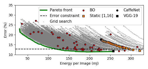
(a) Embedded (local) execution for both networks.

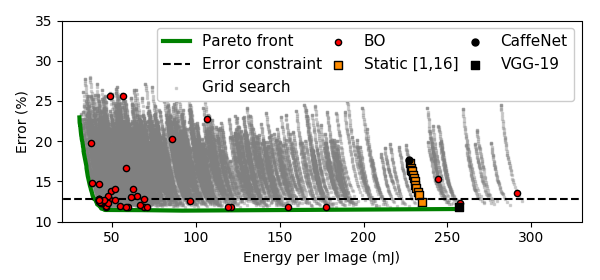
(b) An edge-server energy-minimization design paradigm.

Figure 2. Energy minimization under maximum error constraint. Bayesian optimization considers configurations (red circles) around the near-optimal region, while significantly outperforming static-design systems (orange squares).

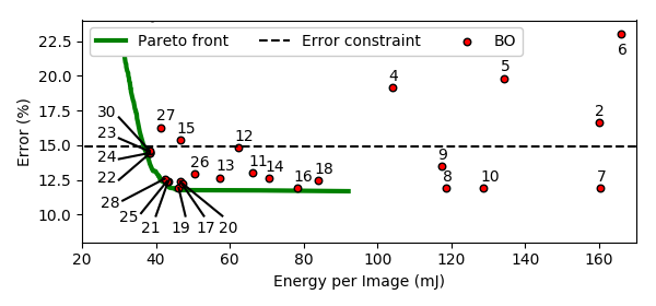
(a) Sequence of configurations selection

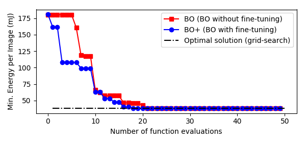
(b) Best solution against the number of function evaluations.

Figure 3. Bayesian optimization for minimum energy under error constraints in the edge-server design. The method progressively evaluates designs closer to the Pareto front. The near-optimal region is reached within 22 function evaluations.

This illustration is insightful and allows us to make three important observations. First, we note how far to the left the Pareto front is compared to the configurations obtained by existing works that optimize only the decision function (orange squares). This fully captures the motivation and novelty behind our work, i.e., to treat the design of adaptive CNN systems as a hyper-parameter problem and globally optimize for the architecture of the CNNs.

Second, it is important to observe that the configurations considered by Bayesian optimization (red circles) lie to the left of both the static optimization designs (orange squares), as well as the monolithic AlexNet and VGG-19 networks (black markers), hence showing that our methodology allows for significant reduction in energy consumption (as discussed in detail next). Third, we note how close to the Pareto-front the Bayesian optimization points are, showing the effectiveness of the method at eventually identifying the feasible, near-optimal region.

Evaluating the effectiveness of BO: To fully assess the effectiveness at reaching the near-optimal region in few tens of function evaluations, we visualize the progress of BO for the case of edge-server adaptive neural networks in Figure 3, which corresponds to the edge-server design of Figure 2(b). First, we show the sequence of configurations selected in Figure 3(a), where we enumerate the first 30 function evaluations. We observe that the near-optimal region is reached with 22 Bayesian optimization steps.

Next, we assess the advantage that the $\kappa$-based fine-tuning step offers. In Figure 3(b), we show the minimum constraint-satisfying energy achieved during Bayesian optimization without (red line) and with (blue line) this step employed during the optimization. In the remainder of the results, we denote these methods as BO and BO⁺, respectively. We also show the optimal solution (dashed line), as obtained by grid search. As motivated in our methodology section, we indeed observe that the fine-tuning step allows the optimization to select configurations around the near-optimal region in less function evaluations. As we discuss in detail next, this is beneficial, especially in over-constrained optimization cases.

Comprehensive adaptive CNNs evaluation: To enable a comprehensive analysis, we employ Bayesian optimization on all three design practices, i.e., local, Ethernet, and wireless. For each design, we solve both a constrained and an over-constrained case for both the error-constrained energy minimization (Equation 3) and the energy-constrained error minimization (Equation 6) problems. We plot the error on the validation set and energy per-image in Figure 4(a) and 4(b), respectively, for both BO and BO⁺. In addition, we compare the optimal result obtained by grid search, the best result by previously published work that treats the CNNs as blackboxes (Park et al., 2015) (denoted as static), and the energy and error by solely using either $N_{1}$ (CaffeNet) or $N_{2}$ (VGG-19) on their own. We report the constraints per case in the parentheses on the x axis.

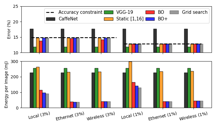
(a) Energy minimization under maximum error constraints.

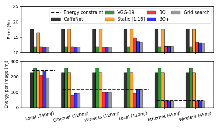
(b) Error minimization under maximum energy constraints.

Figure 4. Assessing the effectiveness of the proposed methodology across different design paradigms and both constrained and over-constrained cases (the constraint values per case are given in the parentheses on the x-axis labels). We observe that our methodology BO⁺ (blue) successfully approaches the grid-search solution (gray), while always outperforming the best solution achieved by existing static-design methods (orange).

Table 1. Hyper-parameter optimization results on the test set. Our methodology does not overfit on the validation set.

	Minimum energy (mJ) achieved under allowed accuracy degradation constraint (given in parenthesis).
Method	Local ($3\%$)	Ethernet ($3\%$)	Wireless ($3\%$)	Local ($1\%$)	Ethernet ($1\%$)	Wireless ($1\%$)
Static (Bolukbasi et al., 2017; Park et al., 2015)	256.09	230.05	231.15	292.25	233.50	235.97
BO	114.43	38.28	41.49	163.15	41.85	45.54
BO+	99.35	38.00	40.50	148.26	41.68	45.54
Grid	93.43	38.00	40.50	123.57	41.68	45.49
	Minimum error (%) achieved under energy constraint (given in parenthesis).
Method	Local ($240mJ$)	Ethernet ($120mJ$)	Wireless ($120mJ$)	Local ($120mJ$)	Ethernet ($45mJ$)	Wireless ($45mJ$)
Static (Bolukbasi et al., 2017; Park et al., 2015)	17.30	18.44	18.44	18.44	18.44	18.44
BO	12.67	12.77	12.74	20.69	12.83	14.42
BO+	12.66	12.70	12.74	16.30	12.83	13.98
Grid	12.58	12.58	12.58	14.14	12.82	13.98

We note that the error percentage value corresponds to the maximum accuracy degradation allowed compared to always using VGG-19 (i.e., the $B$ value in Equation 3). Last, in Figure 4 we report the validation error since this metric is the standard way of assessing the result of Bayesian optimization. We also report the test error of the optimal, feasible solutions obtained in Table 1. Based on the results, we can make several observations:

(i) Suboptimality of prior work: As discussed in the introduction, the energy consumption of CaffeNet and VGG-19 shows a small headroom for energy savings, thereby significantly limiting the effectiveness of the static method. In fact, for local energy minimization with $1\%$ maximum accuracy degradation allowed (similar constraint as in (Park et al., 2015)), statically designed adaptive CNNs will be forced to always use VGG-19 for the final prediction, while wastefully evaluating CaffeNet first. This results in larger energy consumption than using VGG-19 by itself, as seen in Figure 4(a).

(ii) Effectiveness proposed method: We observe that in all the considered cases the proposed BO⁺ method closely matches the result identified by grid search. For instance, in the over-constrained local ($1\%$) case discussed before, Bayesian optimization successfully considers a larger $N_{1}$ configuration that trades-off energy consumption of $N_{1}$, yet improves the overall accuracy such that the error constraint is satisfied.

In general, our methodology identifies designs that outperform static methods (Park et al., 2015) by up to $6\times$ in terms of minimum energy under accuracy constraints and by up to $31.13\%$ in terms of error minimization under energy constraints. Moreover, from Table 1, we confirm the generalization of the methodology, i.e., that the adaptive designs are near-optimal with respect to the test error and that the method does not overfit on the validation set.

(iii) Enhanced performance via $\kappa$-based fine-tuning: As motivated in the methodology section, the fine-tuning step that we incorporate in Bayesian optimization is beneficial especially in the over-constrained cases, allowing the optimization to identify near-optimal regions faster. In particular, BO⁺ leads to further energy minimization under accuracy constraints by $13.18\%$ and to error minimization under energy constraints by $21.22\%$, compared to the result of BO without fine-tuning.

(iv) Local versus remote execution: As an interesting finding in terms of design space exploration, we observe that executing some of CNNs comprising the adaptive neural network remotely allows for more energy-efficient image classification, compared to executing everything locally at the same level of accuracy. Such observations have been also supported by recent design trends which ensure that, due to privacy issues, mobile machine learning services maintain both on-device and cloud components (Leroux et al., 2017; Teerapittayanon et al., 2017; Ko et al., 2018).

We observe this headroom from the Pareto front being further to the left in Figure 2(b) compared to Figure 2(a). That is, using an edge-server design, where only the smallest CNN executes locally, allows for energy reduction of $2.96\times$ compared to executing all networks locally and for the same error constraint. We postulate that this is an interesting finding in terms of computation versus communication trade-offs and an interesting direction to delve into.

Interestingly, we observe that the three-network case is less energy-efficient than using two networks. This is to be expected, since adaptive designs with more networks are better fit for more computationally expensive applications, such as object recognition (Bolukbasi et al., 2017). Exploring the sensitivity of performance metrics to the number of networks is an interesting problem itself. Having shown that our approach can reach near-optimal results compared to exhaustive grid search, we leave this direction for future work.

Table 2. Three-network case: Hyper-parameter optimization results on the test set.

	Minimum energy (mJ) under	Minimum error (%)
Method	accuracy degradation	under energy constraint:
	constraint: Local ($3\%$)	Local ($120mJ$)
Static (Bolukbasi et al., 2017; Park et al., 2015)	268.43	41.25
BO	137.36	17.94
BO+	113.59	15.06
Grid	108.45	14.98

Exploring hierarchy: Finally, we evaluate the proposed method on a three-network case. We summarize the results in Table 2. Once again, we observe that, compared to static methods, our methodology closely matches the results obtained by grid search. More specifically, in the case of energy minimization, the solution reached by $BO^{+}$ is only $4.74\%$ away from the optimal grid search-based design, while outperforming best previously published static methods (Park et al., 2015) by $2.47\times$ in terms of energy minimization.

7. Conclusion

In this paper, we introduced an efficient hyper-parameter optimization methodology to design hardware-constrained adaptive CNNs. The key novelty in our work is that both the architecture settings of the CNNs and the network selection problem are treated as hyper-parameters to be globally (jointly) optimized. To efficiently solve this problem, we enhanced Bayesian optimization to the underlying properties of the design space. Our methodology, denoted as $BO^{+}$, reached the near-optimal region faster compared to a hardware-unaware BO, and the optimal designs identified by grid search.

We exploited the effectiveness of the proposed methodology to consider different adaptive CNN designs with respect to energy, accuracy, and communication trade-offs and constraints imposed by mobile devices. Our methodology identified designs that outperform previously published methods which use CNNs as blackboxes (Park et al., 2015) by up to $6\times$ in terms of minimum energy per image under accuracy constraints and by up to $31.13\%$ in terms of error minimization under energy constraints. Finally, we studied two image classification practices, i.e., classifying all images locally versus over the cloud under energy and communication constraints.

- (1)
- Bolukbasi et al. (2017) Tolga Bolukbasi, Joseph Wang, Ofer Dekel, and Venkatesh Saligrama. 2017. Adaptive Neural Networks for Efficient Inference. In International Conference on Machine Learning. 527–536.
- Cai et al. (2017) Ermao Cai, Da-Cheng Juan, Dimitrios Stamoulis, and Diana Marculescu. 2017. Neuralpower: Predict and deploy energy-efficient convolutional neural networks. arXiv preprint arXiv:1710.05420 (2017).
- Cai et al. (2016) Ermao Cai, Dimitrios Stamoulis, and Diana Marculescu. 2016. Exploring aging deceleration in FinFET-based multi-core systems. In Computer-Aided Design (ICCAD), 2016 IEEE/ACM International Conference on. IEEE, 1–8.
- Chen et al. (2017a) Yu-Hsin Chen, Tushar Krishna, Joel S Emer, and Vivienne Sze. 2017a. Eyeriss: An energy-efficient reconfigurable accelerator for deep convolutional neural networks. IEEE Journal of Solid-State Circuits 52, 1 (2017), 127–138.
- Chen et al. (2017b) Zhuo Chen, Dimitrios Stamoulis, and Diana Marculescu. 2017b. Profit: priority and power/performance optimization for many-core systems. IEEE Transactions on Computer-Aided Design of Integrated Circuits and Systems (2017).
- Dai et al. (2017) Xiaoliang Dai, Hongxu Yin, and Niraj K Jha. 2017. NeST: A Neural Network Synthesis Tool Based on a Grow-and-Prune Paradigm. arXiv preprint arXiv:1711.02017 (2017).
- Ding et al. (2018) Ruizhou Ding, Zeye Liu, RD Shawn Blanton, and Diana Marculescu. 2018. Quantized deep neural networks for energy efficient hardware-based inference. In Design Automation Conference (ASP-DAC), 2018 23rd Asia and South Pacific. IEEE, 1–8.
- Gelbart et al. (2014) Michael A Gelbart, Jasper Snoek, and Ryan P Adams. 2014. Bayesian optimization with unknown constraints. arXiv preprint arXiv:1403.5607 (2014).
- Goodfellow et al. (2013) Ian J Goodfellow, Yaroslav Bulatov, Julian Ibarz, Sacha Arnoud, and Vinay Shet. 2013. Multi-digit number recognition from street view imagery using deep convolutional neural networks. arXiv preprint arXiv:1312.6082 (2013).
- Gordon et al. (2018) Ariel Gordon, Elad Eban, Ofir Nachum, Bo Chen, Hao Wu, Tien-Ju Yang, and Edward Choi. 2018. Morphnet: Fast & simple resource-constrained structure learning of deep networks. In IEEE Conference on Computer Vision and Pattern Recognition (CVPR).
- Han et al. (2015) Song Han, Jeff Pool, John Tran, and William Dally. 2015. Learning both weights and connections for efficient neural network. In NIPS. 1135–1143.
- Hernández-Lobato et al. (2016a) José Miguel Hernández-Lobato, Michael A Gelbart, Ryan P Adams, Matthew W Hoffman, and Zoubin Ghahramani. 2016a. A general framework for constrained Bayesian optimization using information-based search. The Journal of Machine Learning Research 17, 1 (2016), 5549–5601.
- Hernández-Lobato et al. (2016b) José Miguel Hernández-Lobato, Michael A Gelbart, Brandon Reagen, Robert Adolf, Daniel Hernández-Lobato, Paul N Whatmough, David Brooks, Gu-Yeon Wei, and Ryan P Adams. 2016b. Designing neural network hardware accelerators with decoupled objective evaluations. In NIPS workshop on Bayesian Optimization. l0.
- Jia et al. (2014) Yangqing Jia, Evan Shelhamer, Jeff Donahue, Sergey Karayev, Jonathan Long, Ross Girshick, Sergio Guadarrama, and Trevor Darrell. 2014. Caffe: Convolutional architecture for fast feature embedding. arXiv preprint arXiv:1408.5093.
- Ko et al. (2018) Jong Hwan Ko, Taesik Na, Mohammad Faisal Amir, and Saibal Mukhopadhyay. 2018. Edge-Host Partitioning of Deep Neural Networks with Feature Space Encoding for Resource-Constrained Internet-of-Things Platforms. arXiv preprint arXiv:1802.03835 (2018).
- Leroux et al. (2017) Sam Leroux, Steven Bohez, Elias De Coninck, Tim Verbelen, Bert Vankeirsbilck, Pieter Simoens, and Bart Dhoedt. 2017. The cascading neural network: building the Internet of Smart Things. Knowledge and Information Systems 52, 3 (2017), 791–814.
- Panda et al. (2017a) Priyadarshini Panda, Aayush Ankit, Parami Wijesinghe, and Kaushik Roy. 2017a. FALCON: Feature driven selective classification for energy-efficient image recognition. IEEE Transactions on Computer-Aided Design of Integrated Circuits and Systems 36, 12 (2017).
- Panda et al. (2016) Priyadarshini Panda, Abhronil Sengupta, and Kaushik Roy. 2016. Conditional deep learning for energy-efficient and enhanced pattern recognition. In Design, Automation & Test in Europe Conference & Exhibition (DATE), 2016. IEEE, 475–480.
- Panda et al. (2017b) Priyadarshini Panda, Swagath Venkataramani, Abhronil Sengupta, Anand Raghunathan, and Kaushik Roy. 2017b. Energy-efficient object detection using semantic decomposition. IEEE Transactions on Very Large Scale Integration (VLSI) Systems 25, 9 (2017), 2673–2677.
- Park et al. (2015) Eunhyeok Park, Dongyoung Kim, Soobeom Kim, Yong-Deok Kim, Gunhee Kim, Sungroh Yoon, and Sungjoo Yoo. 2015. Big/little deep neural network for ultra low power inference. In Proceedings of the 10th International Conference on Hardware/Software Codesign and System Synthesis. IEEE Press, 124–132.
- Reagen et al. (2017) Brandon Reagen, José Miguel Hernández-Lobato, Robert Adolf, Michael Gelbart, Paul Whatmough, Gu-Yeon Wei, and David Brooks. 2017. A case for efficient accelerator design space exploration via Bayesian optimization. In Low Power Electronics and Design (ISLPED, 2017 IEEE/ACM International Symposium on. IEEE, 1–6.
- Rouhani et al. (2016) Bita Darvish Rouhani, Azalia Mirhoseini, and Farinaz Koushanfar. 2016. Delight: Adding energy dimension to deep neural networks. In Proceedings of the 2016 International Symposium on Low Power Electronics and Design. ACM, 112–117.
- Roy et al. (2018) Deboleena Roy, Priyadarshini Panda, and Kaushik Roy. 2018. Tree-CNN: A Deep Convolutional Neural Network for Lifelong Learning. arXiv preprint arXiv:1802.05800 (2018).
- Russakovsky et al. (2015) Olga Russakovsky, Jia Deng, Hao Su, Jonathan Krause, Sanjeev Satheesh, Sean Ma, Zhiheng Huang, Andrej Karpathy, Aditya Khosla, Michael Bernstein, Alexander C. Berg, and Li Fei-Fei. 2015. ImageNet Large Scale Visual Recognition Challenge. International Journal of Computer Vision (IJCV) 115, 3 (2015), 211–252.
- Smithson et al. (2016) Sean C Smithson, Guang Yang, Warren J Gross, and Brett H Meyer. 2016. Neural networks designing neural networks: multi-objective hyper-parameter optimization. In Proceedings of the 35th International Conference on Computer-Aided Design. ACM, 104.
- Snoek et al. (2012) Jasper Snoek, Hugo Larochelle, and Ryan P Adams. 2012. Practical bayesian optimization of machine learning algorithms. In Advances in neural information processing systems. 2951–2959.
- Stamoulis et al. (2018) Dimitrios Stamoulis, Ermao Cai, Da-Cheng Juan, and Diana Marculescu. 2018. HyperPower: Power-and memory-constrained hyper-parameter optimization for neural networks. In Design, Automation & Test in Europe Conference & Exhibition (DATE), 2018. IEEE, 19–24.
- Stamoulis and Marculescu (2016) Dimitrios Stamoulis and Diana Marculescu. 2016. Can we guarantee performance requirements under workload and process variations?. In Proceedings of the 2016 International Symposium on Low Power Electronics and Design. ACM, 308–313.
- Stamoulis et al. (2015) Dimitrios Stamoulis, Dimitrios Rodopoulos, Brett H. Meyer, Dimitrios Soudris, Francky Catthoor, and Zeljko Zilic. 2015. Efficient Reliability Analysis of Processor Datapath Using Atomistic BTI Variability Models. In Proceedings of the 25th Edition on Great Lakes Symposium on VLSI (GLSVLSI ’15). ACM, 57–62.
- Takhirov et al. (2016) Zafar Takhirov, Joseph Wang, Venkatesh Saligrama, and Ajay Joshi. 2016. Energy-efficient adaptive classifier design for mobile systems. In Proceedings of the 2016 International Symposium on Low Power Electronics and Design. ACM, 52–57.
- Teerapittayanon et al. (2017) Surat Teerapittayanon, Bradley McDanel, and HT Kung. 2017. Distributed deep neural networks over the cloud, the edge and end devices. In Distributed Computing Systems (ICDCS), 2017 IEEE 37th International Conference on. IEEE, 328–339.
- Venkataramani et al. (2015) Swagath Venkataramani, Anand Raghunathan, Jie Liu, and Mohammed Shoaib. 2015. Scalable-effort classifiers for energy-efficient machine learning. In Proceedings of the 52nd Annual Design Automation Conference. ACM, 67.
- Yang et al. (2017) Tien-Ju Yang, Yu-Hsin Chen, and Vivienne Sze. 2017. Designing energy-efficient convolutional neural networks using energy-aware pruning. In IEEE Conference on Computer Vision and Pattern Recognition (CVPR).