Rethinking Pose in 3D: Multi-stage Refinement and Recovery for Markerless Motion Capture

Abstract

We propose a CNN-based approach for multi-camera markerless motion capture of the human body. Unlike existing methods that first perform pose estimation on individual cameras and generate 3D models as post-processing, our approach makes use of 3D reasoning throughout a multi-stage approach. This novelty allows us to use provisional 3D models of human pose to rethink where the joints should be located in the image and to recover from past mistakes. Our principled refinement of 3D human poses lets us make use of image cues, even from images where we previously misdetected joints, to refine our estimates as part of an end-to-end approach. Finally, we demonstrate how the high-quality output of our multi-camera setup can be used as an additional training source to improve the accuracy of existing single camera models.

1 Introduction

One fundamental challenge in the 3D estimation of dynamic and moving objects lies in finding a rich source of ground-truth data. This is not just a problem for modern learning based approaches, that require an abundance of data in order to make inferences about the world, but also for the traditional ones such as model-based reasoning that make heavy use of constraining prior information about the world. Even these traditional methods rely on carefully tuned parameters which control expressiveness of the model [3], internal connectivity priors [26], or both [7] that must be adjusted to recover plausible reconstructions.

Extracting 3D data from images is a fundamentally ill-posed problem that even people find challenging. Unlike standard image labelling problems, such as Imagenet [5], that make heavy use of human annotation, we cannot simply expect people to reliably annotate images with the distance of joints from the camera. The gold standard for accurately capturing 3D information of full-body human poses data remains using Multi-camera Motion Capture (MoCap) systems. These systems make use of early vision techniques based on the identification of markers across multiple cameras and on the estimation of the 3D location of these points through triangulation. However, these systems require strong, unambiguous cues to identify the points. In practice, this means that successful MoCap relies on the subject wearing dark tight clothing and brightly coloured markers, making the captured images unrepresentative of the natural scenes we wish to reconstruct.

In response to these limitations, some recent works [9, 24, 39] have generated more varied synthetic images using MoCap pose data as the source of the human poses. Although these images are more varied than MoCap data, they are still not natural images; and these images tend not to capture information and confusion caused by the deformation of loose fitting clothing [11].

Another approach to avoiding these problems is to chain together different regressors based on multiple data sources; one network is trained to predict 2D joint locations in natural images, while a second regressor upgrades these 2D joint locations to 3D using MoCap data. This approach comes with caveats similar to those of the methods discussed above. We might know that a method gives highly accurate 3D poses on MoCap data and good 2D joint locations in natural images, but we remain fundamentally unsure as to its 3D accuracy in natural images.

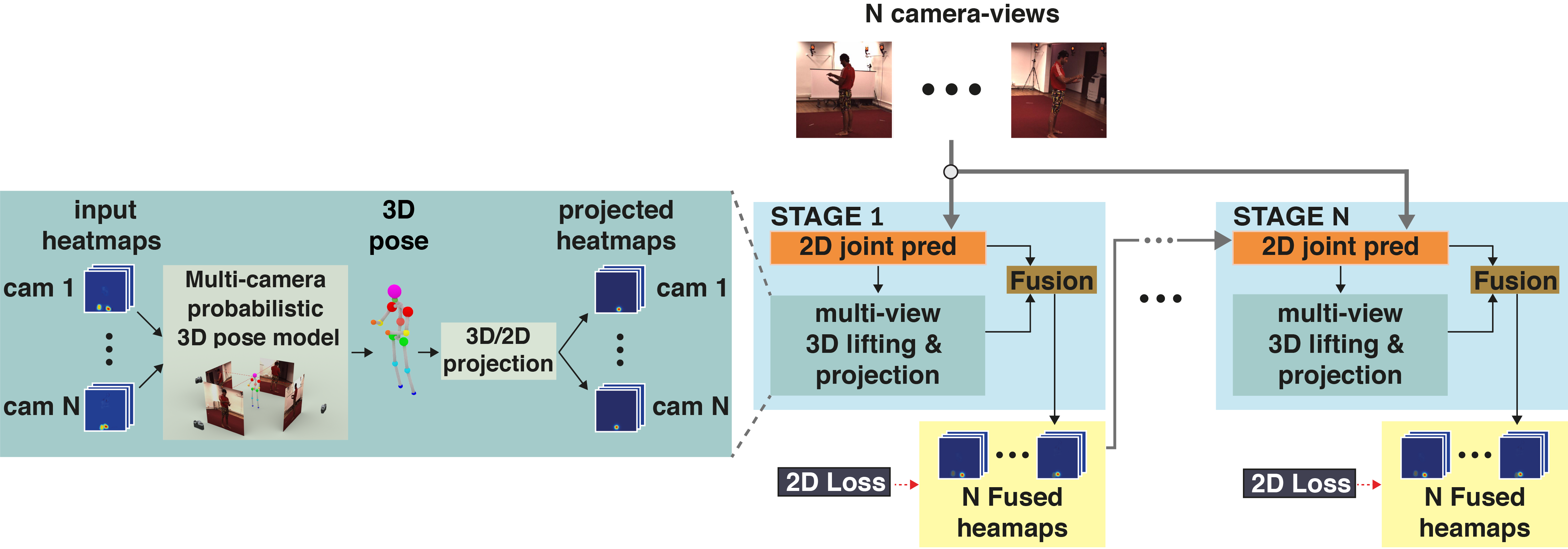
Figure 1: Multi-stage architecture of our proposed multi-camera 3D human pose network. Each stage takes images from all the camera views and the set of per-image 2D joints (expressed as heatmaps) predicted in the previous stage and outputs a refined prediction. In each stage, the 2D predictions from all views are used to reconstruct a single 3D pose, consistent with all camera views. This 3D pose is projected back into the image and used to improve predictions in the next stage. See section 3.1 for more details.

As such, effective markerless motion capture is an important tool to train networks to generate reliable 3D models from natural images. We present a Huber loss based robust estimator for fusing multi-view 2D pose predictions into a coherent 3D pose, consistent with natural human poses. Unlike existing 3D frameworks, this is not simply done at the end of a pipeline for 2D joint estimation, but is iterated through multiple-stages. This carries substantial benefits. Our use of a robust estimator means that at each stage the 3D model can discard a minority of incorrect 2D joint estimates; the knowledge of where the joints should be in each image is fed back into the algorithm for image-based refinement.

One fundamental question regarding these datasets composed of millions of frames, such as Human3.6M, is whether they are in fact large enough. The primary issue is whether the dataset is sufficiently diverse to allow trained networks to exhibit good generalisation to a held-out test set. Even in restrictive cases, such as the test set used in Human3.6M, where the held-out data consists of new actors performing the same movements in similar clothes in the same studio, there is enough variability in individual body shapes and in how they move that generalisation is not guaranteed.

To help address this issue, we demonstrate how unlabelled data can be labelled by our algorithm and augment the datasets used for the training of existing methods, leading to overall better performance on standard benchmarks. We evaluate multiple networks and find consistent multi-millimetre improvement. When the differences between state-of-the-art networks are so small, this raises questions as to whether we are over-fitting and if time would be better spent building larger datasets rather than fighting for small improvements obtained from architectural changes.

Our contribution: We extended existing work on single view reconstruction to a multi-camera setting and show how such single view methods can be enhanced by training on multiview based annotation of unlabelled data. Our use of an iterative, and robust, multistage approach to multi-view reconstruction allows us to correct mistakes in body joint estimations as they arise, and to think again, reconsidering the 2D position of joints in the image using interim knowledge of 3D pose.

Unlike the multiview bootstrapping of Simon et al. [29] which iteratively retrains 2D estimators, our refinement happens at test-time, not training, and only makes use of the information contained in a single set of images captured at one moment in time, rather than requiring extensive retraining on a larger dataset. As such, our approach can be seen as complementary to theirs.

2 Prior Work

Deep convolutional neural networks have led to a substantial improvement in 3D human pose estimation from one or several images. This task is challenging as it involves solving two ill-posed problems: correctly localising the joints of the human body within 2D images and correctly lifting them in 3D. The 2D visual recognition task of localising body joints in the image is made difficult by multiple possible confusing factors including occlusion, variability in the colour, shape and texture of clothing and the lighting conditions, while the task of lifting into 3D is even challenging for humans and intrinsically limited by the existence of perspective ambiguities.

We now review the four most dominant paradigms in monocular 3D human pose estimation: (i) direct image to 3D pose regression; (ii) 3D pose estimation from 2D joint estimates; (iii) joint 2D and 3D pose estimation; and (iv) 3D pose estimation trained on 2D reprojection loss. We also cover recent deep-learning based approaches to multi-view 3D pose estimation.

Direct human 3D pose from a single image: Many recent approaches treat 3D pose estimation from a single input image as a fully supervised learning problem and make use of deep architectures to directly regress the 3D coordinates of human joints from the image  [12, 19, 31, 43]. Much of the novelty of more recent works has involved combining end-to-end learning with expressive 3D priors to constrain the final 3D pose. Li and Chan [12] proposed strategies to jointly train for pose regression and body part detection, Tekin et al. [31] used a pre-trained auto-encoder to enforce structural constraints on the output skeleton. Li et al. [13] trained a deep neural network to predict similarity scores between an input image and a 3D pose using a max-margin loss. Zhou et al. [43] enforce bone lengths in predictions. Tekin et al. also leverage 2D image data [32] by adding a second network stream whose outputs are fused with the 3D regressor. Following the trend in 2D human pose estimation to predict heatmaps rather than regressing 2D landmarks, Pavlakos [20] predicted per-voxel likelihoods, or 3D heatmaps, for each joint using a coarse-to-fine approach.

These methods share the disadvantage of generalising poorly to images in the wild: the need for ground truth 3D poses to train the image to 3D pose regressor means that they must be trained exclusively on images captured in MoCap studios, with all the limitations that come with it.

3D pose from 2D joint estimates: The recent success of 2D pose detection has led to a proliferation of two-stage approaches that estimate 3D human poses from 2D landmarks. Detections are obtained from off-the-shelf 2D pose detectors such as [40, 18, 22]; or included as an initial step in the estimation [14]. The task is then to lift the 2D coordinates into 3D either by model fitting [23, 1, 44, 45, 2, 27] or regression [16, 17]. Moreno-Noguer [17] estimated 3D pose from 2D inputs using 2D-to-3D distance matrix regression. Chen and Ramanan [4] estimated the depth of 2D landmarks by matching them to a library of 3D poses. Bogo et al. [2] fitted a dense statistical shape and pose model, trained on thousands of 3D scans [15], to 2D joints obtained with DeepCut [22]; while Sanzari et al. [27] fitted a non-parametric probabilistic pose model. Martinez et al. [16] show how even a simple regressor - a feed-forward network with residual connections and batch normalization - vastly outperforms previous approaches when given ground truth 2D landmarks as input, suggesting that the largest source of errors in 3D pose reconstruction is incorrect 2D estimation.

Joint 2D-3D pose estimation: Several monocular approaches solve for 2D and 3D pose jointly [28, 32, 25, 30]. Rogez et al. [25] proposed an end-to-end architecture that combines a region proposal network for human localisation with classification and regression branches for joint estimation of 2D and 3D human pose. Sun et al. [30] adopted a bone based representation for the pose and propose a unified setting for 2D and 3D pose estimation that encoded long range interactions between bones. Both approaches achieve best results when a 2D loss is combined with the standard 3D loss. Zhou et al. [42] shared common representations between the 2D and the 3D tasks inside the network which is trained end-to-end with both 2D and 3D losses.

Training with 2D-only loss: A few recent approaches bypass the need to annotate images with 3D ground truth labels by keeping an internal 3D representation of the pose but training based on 2D reprojection losses. These approaches benefit from both their ability to generalise to in-the-wild images as they do not rely on 3D annotated images that can only be captured in studios; and the added structural 3D pose priors afforded by internal 3D representation. Tome et al. [35] proposed a multi-stage architecture that reasons jointly about 2D and 3D pose to improve both tasks. Key to their architecture is a 3D lifting module that reconstructs 2D estimated landmarks in 3D and projects them back into 2D, as their end-to-end training minimises deviations of the reprojected 3D landmarks from the ground truth 2D labels. Wu et al.’s single image 3D interpreter network [41] also uses a loss based on the 2D re-projection error of predicted 3D landmarks, along with a supervised 2D landmarks to 3D pose regressor. Tung et al. [38] combine a similar 2D reprojection loss with an adversarial loss and later [37] propose to combine strong supervision from synthetic data with a self-supervised loss based on consistency checks against 2D estimates of keypoints, segmentation and optical flow.

Multi-view human pose: Elhayek et al. [6] fused 2D body part detections, from a ConvNet-based 2D pose estimation, with a generative model-based multi-view tracking algorithm to reconstruct human pose in indoor and outdoor datasets. Pavlakos et al. [21] proposed a geometry-driven multi-view approach that automatically annotated images with 3D poses starting from generic 2D detections [18]. Their harvested 3D poses are used to demonstrate their effectiveness in two applications: 2D pose personalisation and training a ConvNet from scratch for single view 3D human pose prediction. Trumble [36] made use of a CNN trained on probabilistic visual hull data obtained from multi-viewpoint videos, and an LSTM framework to exploit the temporal continuity of reconstructions.

Unlike approaches such as [6, 21, 36], we do not perform pose estimation for each view before fusing them in a final stage. Instead, we generalise multi-stage approaches[40, 35] to multiple views, and iteratively seek an estimate consistent over all views.

3 Our Formulation

We follow [40, 35] in maintaining a six stage algorithm. At each stage our CNN takes two inputs (see Figure 1): (i) the set of images from different cameras we are trying to reconstruct from; and (ii) the set of 2D pose heatmaps predicted in the previous stage for each multi-view image. Inside each stage the algorithm independently improves the 2D locations of joints in each image and uses them to reconstruct a 3D model consistent with the 2D joint predictions for all the views. Maintaining this internal representation of pose as a 3D model, coherent with all views, allows us to inject 3D information into the learning process. In addition, by reprojecting the 3D model into all the camera views using known camera geometry we can use 2D losses throughout all the stages bypassing the need for 3D annotations associated with the images.

This novel multi-view and multi-stage reconstruction allows us to rethink joint locations in light of knowledge of an interim 3D reconstruction, to recover from mistakes made, and to try again to find support in the image for the predictions of joint locations made by a coherent working hypothesis of 3D positions. Details are given in section 3.1.

Importantly, our approach maintains the computable sub-gradients of Tome et al. [35] when generating and projecting the 3D model. This allows the system to be trained end-to-end. We make substantial changes that improve the robustness of the system while preserving the guarantees of [35] that the model fitting procedure will not get stuck in poor fitting local optima. This is done by replacing the Least Squares procedure of [35] with an Iterative Reweighted Least Squares (irls) approach that mimics the Huber loss and preserves convexity for any particular choice of planar rotation. Details of this are given in section 3.4.

3.1 Details of the Network

Our proposed architecture is a multi-stage convolutional neural network inspired by the work of Tome et al. [35], which was in turn an extension of the architecture introduced by Wei et al. [40]. They proposed Convolutional Pose Machines (CPM), a multi-stage 2D pose estimator in which each stage performed a refinement of the estimate computed by the previous stage.

As shown in Figure 1, the first step in each stage independently predicts, in every camera view, the 2D pose of the person in the image. These predictions take the form of heatmaps generated via a convolutional architecture with the weights shared between all camera views.

These heatmaps are generated by a: (a) a set of convolutional layers shared by all stages that are performing feature extraction; followed by (b) a set of convolutional layers, unique to each stage, that compute a heat map representing the location of each joint. All stages (except stage 1) also take as input the heatmaps generated in the previous stage. The size and connections of these convolutional layers remain the same as in CPM[40]. However, we additionally apply batch normalization before the ReLu.

The next step within each stage takes heat-maps as input and computes the 3D pose most consistent with the 2D information provided by each camera view. Heat-maps are then converted into 2D locations by selecting the most confident pixel as the location of each of the joints

$$I_{p}^{c}=\operatorname*{arg\,max}_{(u,v)}H_{p}^{c}[u,v]$$

where $H_{p}^{c}$ is the heat-map representing joint $p$ for camera view $c$. These 2D poses are then used by the multi-camera probabilistic 3D pose estimator (described in section 3.4) to generate a single 3D pose that agrees over all the different camera 2D poses. This pose is projected back onto the 2D image for each camera view using a weak perspective projection, and the new projected 2D poses are converted into heat-maps by a Gaussian convolution

$$\hat{H}_{p}^{c}[u,v]=\begin{cases}1&\text{if}(u,v)=\hat{I}_{p}^{c}\\ 0&\text{otherwise.}\end{cases}$$

where $\hat{I}_{p}^{c}$ is joint $p$ of the projected 2D pose in camera $c$.

The final operation fuses the heat-maps regressed by the convolutional layers with those estimated by projecting the 3D pose into 2D. This fusion is implemented by applying a convolutional layer with filters of size $\left[1\times 1\right]$ and number_joints filters, to each camera view independently, giving a set of heatmaps, one for each choice of joint and camera.

As an implementation detail, all the computations performed on each camera view make use of the same convolutional operations; this enables us to have an efficient implementation by setting the batch size to be equal to the number of cameras and ordering the images appropriately.

3.2 Studio Setup and Camera Assumptions

We make use of the Human3.6M dataset [9] for training and evaluation. This dataset was generated in a multi-source capture studio with the ground-truth reconstructions coming from a ten camera Vicon studio, and four video cameras facing each another at right angles and far enough to fully capture a 4 by 3 meter studio environment.

Following the camera model and inference of [35], we continue to assume a scaled orthographic model. Importantly, we assign the same choice of scale to all cameras. This assumption is noticeably stronger than the previous scaled orthographic reconstruction of [35]. With the four cameras facing towards each other, our stronger assumption does not allow increase in overall scale due to movements towards one camera, as this would correspond with movement away from another camera and a corresponding decrease in scale. However, it does allow for changes in scale of the object itself allowing our algorithm to handle people of different sizes.

3.3 Additional data

One concern, when trying to show how additional data can lead to improved results in the 3D reconstruction of people, is the restrictive form of the Human3.6M evaluation dataset. With the limited appearance and repetitive range of actions, that occur both in the training and in the evaluation sets, networks trained on more general datasets might perform worse than those trained on restrictive datasets that are closer to the test data. To avoid such issues, we make use of an additional set of actors performing the same actions captured by the authors of the Human3.6M dataset.

As with many datasets in computer vision, Human3.6M was originally subdivided into training, test and validation subsets; the reconstructions for the test set were not made publicly available, to avoid over-fitting. However, for historic reasons, the test set has gone largely unused, with detailed evaluations being reported on the validation set. This means that we have access to a publicly available additional corpus, composed of unlabelled images from 2 men and 1 woman, captured in the same environment.

To illustrate how 3D data gathered by our method can improve existing results, we augment two existing networks using this data. Our results show clear improvement over published results, and help make the case not just that better networks are needed for better results, but also more data.

Additional data can help 3D predictions in two separate ways, either by improving the 2D localisation of joints, or by improving the 3D lifting from the same 2D inputs. To show that our method returns results of sufficiently high quality to improve both components, we perform two separate experiments: (1) we show improvements on 2D joint prediction while keeping the 3D lifting constant, and (2) we show how a generic lifter that takes as input precomputed joint locations can be improved by training on our additional 3D data.

3.4 3D pose estimation

We now review the pose estimation of Tome et al.[35] that generates a 3D pose from 2D joint locations; discuss its generalisation to multi-camera systems; and modifications to improve robustness to outliers and its stability.

Tome et al. suggested approaching human pose estimation using a formulation inspired by non-rigid structure from motion. Assuming a known basis of human poses given by a set of matrices ${\bf e}$, and standard deviations $\sigma$, and a rest shape $\mu$, they suggest estimating the cost of a particular parameterised human pose, given 2D locations $I$, as:

$$\operatorname*{arg\,min}_{R,a}||I-s\Pi ER(\mu+a\cdot{\bf e})||_{2}^{2}+\sigma^{2}\cdot a^{2}$$ (1)

Where $\Pi$ is the canonical orthographic projection matrix, $E$ a known transformation from the world co-ordinates to those of the camera, $R$ is a planar rotation matrix that describes the rotation of the human pose in the ground-plane, and $s$ is the estimated per-frame scale. Here $a$ is a vector of basis coefficients, ${\bf e}$ a 3D tensor of dimensions basis $\times$ points $\times$ 3. The tensor product $a\cdot{\bf e}$ is defined as $\sum_{i}a_{i}{\bf e}_{i}$, and the square terms in the final expression refer to an elementwise square. The closest parameterised pose for 2D data $I$ was given by minimising the cost:

$$\operatorname*{arg\,min}_{s,a,R}P(s,a,R|I)$$ (2)

The authors observed that, for any given choice of rotation, the global minima could be interpreted as an unconstrained linear least squares problem and solved efficiently. They suggested brute forcing over a small set of ground plane rotations to quickly find a global minima without needing to worry about getting stuck in poor quality local optima.

We make several additions to this framework:

3.4.1 Rotation marginalisation for improved stability

Tome et al. [35] observed that using more than $80$ rotations did not improve the overall accuracy of the reconstructions. Although this is true, their algorithm often yields flickering and unstable reconstructions when run on video data. Much of this flicker can be attributed towards trying to reconstruct ambiguous poses that can be equally well explained by two or more different rotations. We write the optimal reconstruction given a choice of rotation $R$ as $Q_{R}=Rs(\mu+a\cdot{\bf e})$ where $a$, and $s$ are found by solving the following optimisation problem

$$\{s,a\}=\operatorname*{arg\,min}_{s,a}P(s,a,R|I)$$ (3)

Marginalising over the set of rotations $\cal R$, gives the following 3D body pose estimate:

$$\frac{\sum_{R\in\cal R}\exp(-\rho P(s_{R},a_{R},R|I))Q_{R}}{\sum_{R\in\cal R}\exp(-\rho P(s_{R},a_{R},R|I))}$$ (4)

This elimination of flickering is highly desirable, not just in that it makes the reconstructions of video appear more lifelike and appealing to humans, but also in that the stability of the reconstructions carries important semantic information. If we are to use 3D reconstructions of people as a first step in action analysis, the stability and dynamics of the reconstructions contains important information that informs our understanding of the actions.

3.4.2 Principled shape warping for multiple views

Tome et al. [35], approached the problem of reconstruction through the lens of probabilistic PCA [34] with a known basis. In their framework, after generating a reconstruction from basis coefficients, a final stage is to warp the reconstruction to lie closer to the input data. In the context of 3D reconstruction from an single orthographic camera this can be done as post processing, where a weighted average of the $x$ and $y$ coefficients of the image and the reconstruction $Q_{R}$ are taken together while the $z$ component remains constant.

When multiple cameras are being used, this fusion between the model and the data can not be performed as a simple post-processing step. Instead, we jointly estimate a new shape $\tilde{Q}$ consistent with all frames and close to the model estimate. Given a rotation $R$, this can be written as

$$\operatorname*{arg\,min}_{\tilde{Q}_{R},s,a}\lambda\sum_{c\in\cal C}||I_{C}-\Pi E\tilde{Q}_{R}||_{2}^{2}+||\tilde{Q}_{R}-sR(\mu+a\cdot{\bf e})||_{2}^{2}+\sigma^{2}\cdot a^{2}$$ (5)

where $\cal C$ refers to a set of cameras, $\lambda$ is a known scale factor, and $E$ is the known external calibration that aligns world co-ordinates with the camera’s frame of reference. As is standard in geometry, this formulation finds the single body pose that best explains all viewpoints; this is not equivalent to applying a single camera approach to each view and averaging the results. Again, this can be directly solved as an unconstrained least squares problem given $R$; and as discussed in the previous subsection, we continue to marginalise over the space of rotations.

3.4.3 Robust losses for outlier rejection

Finally, the use of the squared Frobenius norm as in the previous section makes the reconstruction less robust to occlusions and to misdetected joints. If the camera views were aligned, the first term of (5) would be minimised by a pose that averages over the different predictions. Use of the Frobenius norm would mean that if only one prediction is in the wrong place, it would “pull” the reconstruction towards the mistake rather than discarding it as an outlier. Instead we replace the squared Frobenius norm with a Huber loss.

$$\operatorname*{arg\,min}_{\tilde{Q}_{R},s,a}\lambda\sum_{c\in\cal C}||I_{c}-\Pi E\tilde{Q}_{R}||_{\epsilon}+||\tilde{Q}_{R}-sR(\mu+a\cdot{\bf e})||_{2}^{2}+\sigma^{2}\cdot a^{2}$$ (6)

where the Huber Loss $||x||_{\epsilon}=\sum_{i}|x_{i}|_{\epsilon}$ and

$$|x|_{\epsilon}=\begin{cases}\frac{|x_{i}|^{2}}{2}&\text{if $|x_{i}|\leq\epsilon$}\\ \epsilon|x_{i}|-\frac{\epsilon^{2}}{2}&\text{ otherwise.}\end{cases}$$ (7)

Although (6) is not a least square problem, it can be solved as an iterative reweighted least squares problem (irls). In practice, 5 iterations of least squares are sufficient to obtain a high quality solution. Although robust to outliers, this new loss remains convex given a choice of rotation, so local minima are not a concern. The use of irls for a fixed number of iterations allows gradient propagation and end-to-end training as in [35].

4 Refining Existing Monocular Networks

Given the noticeable improvement in accuracy obtained by using multiple cameras rather than just one (see table 1), it is natural to ask if our results can improve the performance of existing networks by labelling previously unlabelled data, and using this to augment the training set. This labelling of new data can be seen in Figure 2.

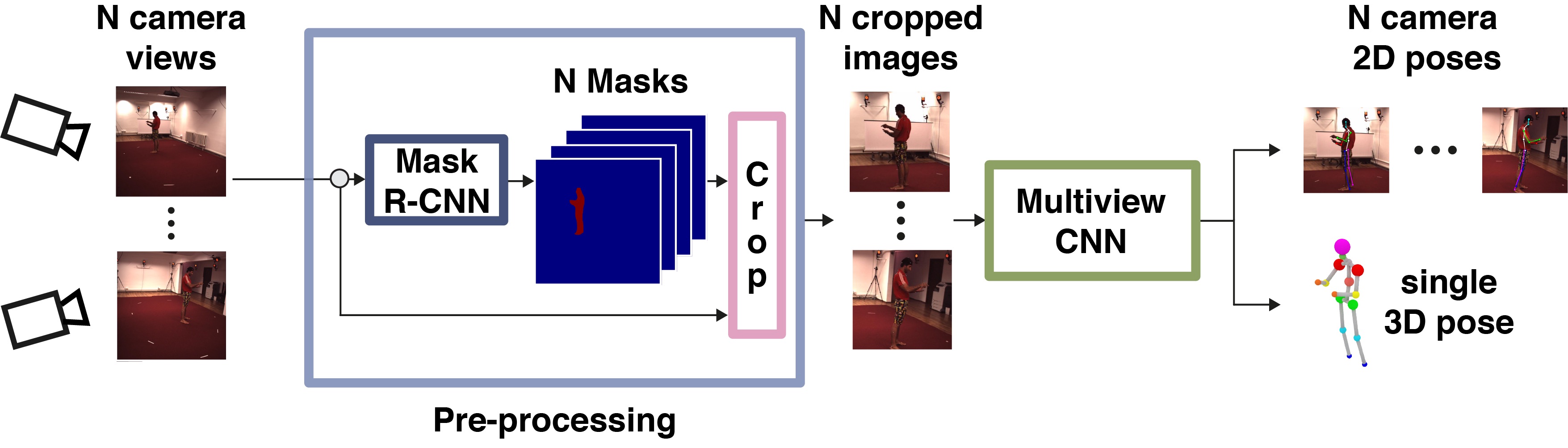
Figure 2: Labelling data using multi-camera 3D pose estimator.

Although conceptually simple, multiple small issues arise from most experiments reporting results on an automatically preprocessed version of the Human3.6M dataset. First, images are independently run through the Mask R-CNN architecture [8] in order to extract both the bounding box and the silhouette of the person represented in the images. This information is essential for cropping the area of the image containing the person in a similar manner to what is done on images with ground truth 2D data, guaranteeing that: 1) all the joints are inside the cropped region, centred around the hips; 2) the aspect ratio is one and 3) $25$ pixels of margin are added to the cropped region. These cropped regions are then used as inputs to our multi-camera network which estimates 2D body poses for each camera view and identifies the 3D pose most consistent with the set of 2D poses. Finally, the 3D pose is projected into 2D for each camera view using the known camera calibration.

Data labelled by our approach is used to extend existing datasets. We simply treat the predicted bounding-boxes, 2D landmarks and 3D reconstructions the same way as existing ground truth training data.

5 Experiments

Protocol 1	Dir.	Disc.	Eat	Greet	Phone	Photo	Pose	Purch.	Sit	SitD.	Smoke	Wait	WalkD.	Walk	WalkT.	Avg
LinKDE [9]	132.7	183.6	132.4	164.4	162.1	205.9	150.6	171.3	151.6	243.1	162.1	170.7	177.1	96.6	127.9	162.1
Li et al. [13]	-	136.9	96.9	124.7	-	168.7	-	-	-	-	-	-	132.1	69.9	-	-
Tekin et al. [33]	102.4	158.5	87.9	126.8	118.4	185.1	114.7	107.6	136.2	205.7	118.2	146.7	128.1	65.9	77.2	125.3
Zhou et al. [45]	87.4	109.3	87.1	103.2	116.2	143.3	106.9	99.8	124.5	199.2	107.4	118.1	114.2	79.4	97.7	113.0
Tome et al. [35]	64.9	73.5	76.8	86.4	86.3	110.7	68.9	74.8	110.2	172.9	84.9	85.8	86.3	71.4	73.1	88.4
Pavlakos et al. [20]	67.4	71.9	66.7	69.1	72.0	77.0	65.0	68.3	83.7	96.5	71.7	65.8	74.9	59.1	63.2	71.9
Tekin et al. [32]	53.9	62.2	61.5	66.2	80.1	79.5	64.6	83.2	70.9	107.9	70.4	68.0	77.8	52.8	63.1	70.8
Katircioglu et al. [10]	54.9	63.3	57.3	62.3	70.3	77.4	56.7	57.1	79.0	97.1	64.3	61.9	67.1	49.8	62.3	65.4
Zhou et al. [42]	54.8	60.7	58.2	71.4	62.0	65.5	53.8	55.6	75.2	111.6	64.15	66.05	51.4	63.2	55.3	64.9
Martinez et al. [16]	51.8	56.2	58.1	59.0	69.5	78.4	55.2	58.1	74.0	94.6	62.3	59.1	65.1	49.5	52.4	62.9
Multi-View Martinez	46.5	48.6	54.0	51.5	67.5	70.7	48.5	49.1	69.8	79.4	57.8	53.1	56.7	42.2	45.4	57.0
PVH-TSP [36]	92.7	85.9	72.3 7	93.2	86.2	101.2	75.1	78.0	83.5	94.8	85.8	82.0	114.6	94.9	79.7	87.3
Pavlakos et al. [21]	41.2	49.2	42.8	43.4	55.6	46.9	40.3	63.7	97.6	119.0	52.1	42.7	51.9	41.8	39.4	56.9
Ours	43.3	49.6	42.0	48.8	51.1	64.3	40.3	43.3	66.0	95.2	50.2	52.2	51.1	43.9	45.3	52.8

Table 1: Quantitative evaluation on the Human3.6M dataset. We report 3D pose error results expressed in mm using the metric defined in protocol 1. All methods above the first line are monocular while those below ( [36, 21] and Ours) are multi-camera approaches. ‘’Multi-View Martinez” refers to independently reconstructing from each monocular view using [16] followed by averaging.

We evaluate on Human3.6M using the two standard protocols for evaluation. In protocol 1, the training set consists of 5 subjects (S1, S5, S6, S7, S8), whereas the test set includes subjects (S9, S11). The error metric is the Euclidean distance from the estimated 3D joints to the ground truth, averaged over all 17 joints of the Human3.6M skeletal model, and without alignment. The evaluation is performed every $5^{\text{th}}$ frame, as in [45], due to the high similarity of subsequent frames.

Protocol 2, introduced by Bogo et al. [2], uses the same training and testing set as protocol 1. However, evaluation is performed on all frames captured by camera 3 during trial 1, and the error metric reported is the average per-joint 3D error after aligning the reconstruction with the ground-truth using Procrustes analysis.

Table 1 shows a comparison of our multi-camera approach with other state-of-the-art techniques (both monocular and multi-view) under protocol 1. Our proposed approach outperforms monocular methods, reducing the error by over $10$ milimetres, and gives better results than the best multi-camera method of Pavlakos et al. [21] with an improvement of more than $4$ milimetres. We also create a novel baseline based on generating monocular reconstructions from each view using the method of Martinez et al. [16], and averaging them after alignment. This performs almost as well as Pavlakos et al., and is reported in table 1 as “Multi-view Martinez”. Table 2 shows a comparison with other state of the art approaches using protocol 2.

Protocol 2	Dir.	Disc.	Eat	Greet	Phone	Photo	Pose	Purch.	Sit	SitD.	Smoke	Wait	WalkD.	Walk	WalkT.	Avg
Akhter & Black [1] 14j	199.2	177.6	161.8	197.8	176.2	186.5	195.4	167.3	160.7	173.7	177.8	181.9	176.2	198.6	192.7	181.1
Ramakrishna et al. [23] 14j	137.4	149.3	141.6	154.3	157.7	158.9	141.8	158.1	168.6	175.6	160.4	161.7	150.0	174.8	150.2	157.3
Zhou et al. [44] 14j	99.7	95.8	87.9	116.8	108.3	107.3	93.5	95.3	109.1	137.5	106.0	102.2	106.5	110.4	115.2	106.7
Bogo et al. [2] 14j	62.0	60.2	67.8	76.5	92.1	77.0	73.0	75.3	100.3	137.3	83.4	77.3	86.8	79.7	87.7	82.3
Tome et al. [35] 14j	-	-	-	-	-	-	-	-	-	-	-	-	-	-	-	79.6
Moreno-Noguer [17] 14j	66.1	61.7	84.5	73.7	65.2	67.2	60.9	67.3	103.5	74.6	92.6	69.6	71.5	78.0	73.2	74.0
Ours 14j	40.4	42.8	39.8	44.8	47.5	59.1	36.6	37.0	55.8	82.3	46.8	48.9	48.2	38.8	40.4	47.6
Pavlakos et al. [20] 17j	-	-	-	-	-	-	-	-	-	-	-	-	-	-	-	51.9
Martinez et al. [16] 17j	39.5	43.2	46.4	47.0	51.0	56.0	41.4	40.6	56.5	69.4	49.2	45.0	49.5	38.0	43.1	47.7
Ours 17j	38.2	40.2	38.8	41.7	44.5	54.9	34.8	35.0	52.9	75.7	43.3	46.3	44.7	35.7	37.5	44.6

Table 2: Quantitative evaluation of our approach against other methods using protocol 2 on the Human3.6M dataset. Note that all other methods are monocular. The $14j$/$17j$ annotation indicates the number of joints used in evaluation.

Formulation	Error Protocol 1	Error Protocol 2
Squared Frobenius (no averaging)	59.6 mm	51.1 mm
Squared Frobenius	59.4 mm	51.8 mm
Huber loss	52.8 mm	44.6 mm
Huber loss (2 cameras)	64.2 $\pm$ 1.6 mm	52.8 $\pm$ 1.4 mm
GT Orthographic Triangulation	27.9 mm	20.7 mm

Table 3: Reconstruction error for different variants of our approach (see section 3.4 for details.) Huber loss (2 cameras) shows the mean and standard deviation of the reconstruction using only a pair of cameras at right angles with one another. GT Orthographic Triangulation shows the error due to the use of an orthographic camera, i.e. the the reconstruction error given perfect detections.

Table 3 shows the importance of the changes to the pose estimation made in 3.4; particularly the use of a more robust Huber loss in place of the squared Frobenius norm, (Eq. 5 and Eq. 6). Although, many works make use of the Huber loss as a more stable approximation of the $\ell_{1}$ norm, this is not the case for us. Upon inspection, we found that the optimal choice of $\epsilon$ that resulted in the lowest 3D reconstruction error treated half of the joints with $\ell_{1}$ norm and the other half with the squared Frobenius norm which confirms that the Huber loss is effectively used to weigh the relevance of each joint on a case by case basis.

A small improvement can also be seen from marginalising over the rotations, although this modification primarily improves the stability of reconstructions rather than reducing the overall error. Finally we show how much error can be attributed to the camera model, by triangulating ground-truth detections under orthographic assumptions. This is reported as “GT Orthographic Triangulation”.

5.1 Improving Existing Monocular 3D Pose Networks

Table 4 shows the results of existing pose estimation techniques [35, 16] evaluated on a variety of experiments where the models were trained using ground-truth training data provided by the Human3.6M dataset [9], and additional unlabelled data (Subjects $\{S2,S3,S4\}$), automatically labelled as previously described in section 3.3.

In both approaches, we took the training hyper-parameters provided by the papers and retrained the respective models using the augmented training data, without fine-tuning the hyper-parameters.

The authors of [16] no longer have access to the retrained stacked-hourglass 2D networks that they take as an input, so we can not compute their 2D joint estimations on the held-out unlabelled data. Instead we repeat their experiments, by training the network using the 2D poses estimated by Tome et al. [35] as input, and using these inputs to drive the 3D prediction. Without optimising the hyperparameters, this leads to a noticeable decrease in the performance of the algorithm over that reported by their paper, even though Tome et al. report a lower 2D error than that of Martinez et al. Despite this, we still observe a substantial improvement in the 3D reconstruction from using more data. Note that for this experiment, we do not update the 2D pose estimations, and all improvement comes from the updated 3D estimator.

To illustrate that our method also improves 2D joint localisation, we also retrain the network of Tome et al. As an initial step in training the algorithm, Tome et al. compute a shape basis from MoCap data. This basis is not updated during the end-to-end training of the pose estimator, and the network itself is trained to improve 2D loss in joint predictions, returning a 3D pose as a side-effect of its 2D pose computation. Although we could update the 3D basis using our newly labelled data, we restrict ourselves to only updating the 2D pose predictor. As can be seen in table 4, this leads to a significant improvement in 2D error, and a corresponding reduction in the 3D error.

Approach	Experiment	Human3.6M dataset		$\Delta$	%
		Train	Train + new data
Tome et al.	3D error (P#1)	88.4 mm	84.4 mm	4.0	4.52
[35]	3D error (P#2)	70.7 mm	67.2 mm	3.5	4.95
	2D error	9.5 pix	8.6 pix	0.9	9.47
Martinez et al.	3D error (P#1)	75.8 mm	72.5 mm	3.3	4.35
[16]	3D error (P#2)	57.6 mm	55.9 mm	1.7	2.95

Table 4: Quantitative evaluation performed on existing approaches, demonstrating the performance gain when various models are trained with our additional data.

Figure 3 shows some sampled 2D and 3D poses with the respective reconstruction error for some multi-camera frames taken from the test-set of Human3.6M dataset. The sorted error plot is based on sampling the error every $10^{\text{th}}$ frame of trial 1.

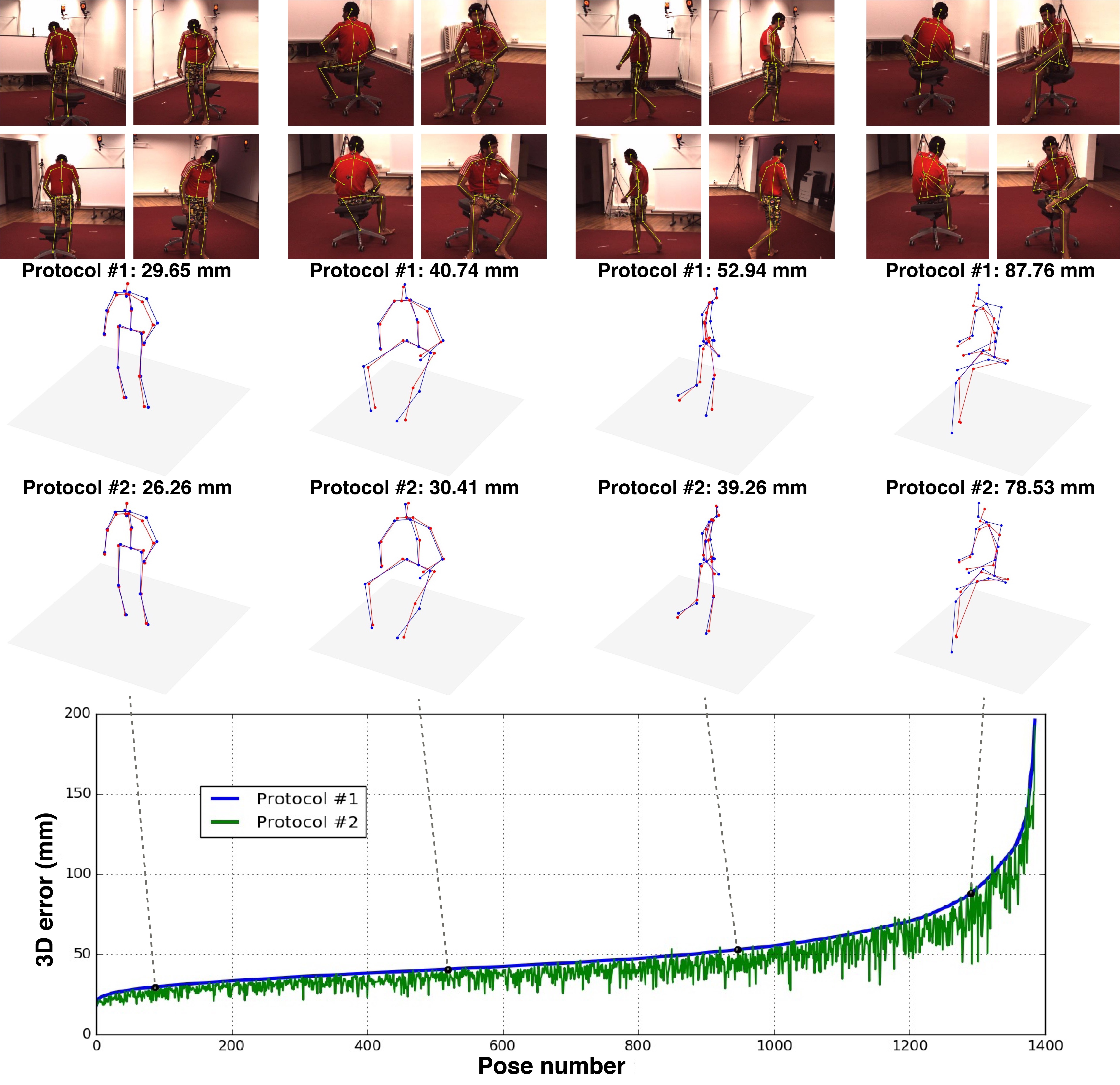
Figure 3: Multi-camera reconstructions showing sampled 3D errors from the test-set, sorted from small to large, for both protocol 1 and protocol 2. Ground-truth reconstructions are given in blue, and the rows labelled protocol 1 and protocol 2 both show the same reconstructions in red, however protocol 1 shows the reconstruction unaligned with the ground-truth, and protocol 2 shows the reconstruction aligned to the ground-truth. See section 5 for more details of the protocols.

6 Conclusion

We have shown a novel approach to markerless multi-camera motion-capture with a multi-stage architecture that allows us to recover from initial misdetections, and still make use of image cues in locating joints in subsequent stages.

We have demonstrated the clear benefits and robustness of our approach by noticeably improving over existing multi-view markerless motion capture system. In addition to this, we have shown how existing methods can be improved by using our approach as an initial first step to label otherwise unlabelled data.

References

- [1] I. Akhter and M. J. Black. Pose-conditioned joint angle limits for 3d human pose reconstruction. In Proceedings of the IEEE Conference on Computer Vision and Pattern Recognition, pages 1446–1455, 2015.
- [2] F. Bogo, A. Kanazawa, C. Lassner, P. Gehler, J. Romero, and M. J. Black. Keep it smpl: Automatic estimation of 3d human pose and shape from a single image. In European Conference on Computer Vision, pages 561–578. Springer, 2016.
- [3] C. Bregler, A. Hertzmann, and H. Biermann. Recovering non-rigid 3d shape from image streams. In Computer Vision and Pattern Recognition, 2000. Proceedings. IEEE Conference on, volume 2, pages 690–696. IEEE, 2000.
- [4] C.-H. Chen and D. Ramanan. 3d human pose estimation= 2d pose estimation+ matching. In 2017 IEEE Conference on Computer Vision and Pattern Recognition (CVPR). IEEE, 2017.
- [5] J. Deng, W. Dong, R. Socher, L.-J. Li, K. Li, and L. Fei-Fei. Imagenet: A large-scale hierarchical image database. In Computer Vision and Pattern Recognition, 2009. CVPR 2009. IEEE Conference on, pages 248–255. IEEE, 2009.
- [6] A. Elhayek, E. de Aguiar, A. Jain, J. Tompson, L. Pishchulin, M. Andriluka, C. Bregler, B. Schiele, and C. Theobalt. Efficient convnet-based marker-less motion capture in general scenes with a low number of cameras. In Computer Vision and Pattern Recognition (CVPR), 2015 IEEE Conference on, pages 3810–3818. IEEE, 2015.
- [7] R. Garg, A. Roussos, and L. Agapito. Dense variational reconstruction of non-rigid surfaces from monocular video. In Computer Vision and Pattern Recognition (CVPR), 2013 IEEE Conference on, pages 1272–1279. IEEE, 2013.
- [8] K. He, G. Gkioxari, P. Dollár, and R. Girshick. Mask r-cnn. In Computer Vision (ICCV), 2017 IEEE International Conference on, pages 2980–2988. IEEE, 2017.
- [9] C. Ionescu, D. Papava, V. Olaru, and C. Sminchisescu. Human3. 6m: Large scale datasets and predictive methods for 3d human sensing in natural environments. IEEE transactions on pattern analysis and machine intelligence, 36(7):1325–1339, 2014.
- [10] I. Katircioglu, B. Tekin, M. Salzmann, V. Lepetit, and P. Fua. Learning latent representations of 3d human pose with deep neural networks. International Journal of Computer Vision, pages 1–16, 2018.
- [11] C. Lassner, G. Pons-Moll, and P. V. Gehler. A generative model of people in clothing. arXiv preprint arXiv:1705.04098, 2017.
- [12] S. Li and A. B. Chan. 3d human pose estimation from monocular images with deep convolutional neural network. In Asian Conference on Computer Vision, pages 332–347. Springer, 2014.
- [13] S. Li, W. Zhang, and A. B. Chan. Maximum-margin structured learning with deep networks for 3d human pose estimation. In Proceedings of the IEEE International Conference on Computer Vision, pages 2848–2856, 2015.
- [14] M. Lin, L. Lin, X. Liang, K. Wang, and H. Cheng. Recurrent 3d pose sequence machines. In Proceedings of the IEEE Conference on Computer Vision and Pattern Recognition, pages 810–819, 2017.
- [15] M. Loper, N. Mahmood, J. Romero, G. Pons-Moll, and M. J. Black. Smpl: A skinned multi-person linear model. ACM Transactions on Graphics (TOG), 34(6):248, 2015.
- [16] J. Martinez, R. Hossain, J. Romero, and J. J. Little. A simple yet effective baseline for 3d human pose estimation. In IEEE International Conference on Computer Vision, volume 206, page 3, 2017.
- [17] F. Moreno-Noguer. 3d human pose estimation from a single image via distance matrix regression. In 2017 IEEE Conference on Computer Vision and Pattern Recognition (CVPR), pages 1561–1570. IEEE, 2017.
- [18] A. Newell, K. Yang, and J. Deng. Stacked hourglass networks for human pose estimation. In European Conference on Computer Vision, pages 483–499. Springer, 2016.
- [19] S. Park, J. Hwang, and N. Kwak. 3d human pose estimation using convolutional neural networks with 2d pose information. In European Conference on Computer Vision, Workshops, pages 156–169. Springer, 2016.
- [20] G. Pavlakos, X. Zhou, K. G. Derpanis, and K. Daniilidis. Coarse-to-fine volumetric prediction for single-image 3d human pose. In Computer Vision and Pattern Recognition (CVPR), 2017 IEEE Conference on, pages 1263–1272. IEEE, 2017.
- [21] G. Pavlakos, X. Zhou, K. G. Derpanis, and K. Daniilidis. Harvesting multiple views for marker-less 3d human pose annotations. In Proceedings of the IEEE Conference on Computer Vision and Pattern Recognition, pages 6988–6997, 2017.
- [22] L. Pishchulin, E. Insafutdinov, S. Tang, B. Andres, M. Andriluka, P. V. Gehler, and B. Schiele. Deepcut: Joint subset partition and labeling for multi person pose estimation. In Proceedings of the IEEE Conference on Computer Vision and Pattern Recognition, pages 4929–4937, 2016.
- [23] V. Ramakrishna, T. Kanade, and Y. Sheikh. Reconstructing 3d human pose from 2d image landmarks. In European Conference on Computer Vision, pages 573–586. Springer, 2012.
- [24] G. Rogez and C. Schmid. Mocap-guided data augmentation for 3d pose estimation in the wild. In Advances in Neural Information Processing Systems, pages 3108–3116, 2016.
- [25] G. Rogez, P. Weinzaepfel, and C. Schmid. Lcr-net: Localization-classification-regression for human pose. In CVPR 2017-IEEE Conference on Computer Vision & Pattern Recognition, 2017.
- [26] C. Russell, R. Yu, and L. Agapito. Video pop-up: Monocular 3d reconstruction of dynamic scenes. In European conference on computer vision, pages 583–598. Springer, 2014.
- [27] M. Sanzari, V. Ntouskos, and F. Pirri. Bayesian image based 3d pose estimation. In European Conference on Computer Vision, pages 566–582. Springer, 2016.
- [28] E. Simo-Serra, A. Quattoni, C. Torras, and F. Moreno-Noguer. A joint model for 2d and 3d pose estimation from a single image. In Computer Vision and Pattern Recognition (CVPR), 2013 IEEE Conference on, pages 3634–3641. IEEE, 2013.
- [29] T. Simon, H. Joo, I. A. Matthews, and Y. Sheikh. Hand keypoint detection in single images using multiview bootstrapping. CoRR, abs/1704.07809, 2017.
- [30] X. Sun, J. Shang, S. Liang, and Y. Wei. Compositional human pose regression. In The IEEE International Conference on Computer Vision (ICCV), volume 2, 2017.
- [31] B. Tekin, I. Katircioglu, M. Salzmann, V. Lepetit, and P. Fua. Structured prediction of 3d human pose with deep neural networks. In British Machine Vision Conference (BMVC), 2016.
- [32] B. Tekin, P. Marquez-Neila, M. Salzmann, and P. Fua. Learning to fuse 2d and 3d image cues for monocular body pose estimation. In The IEEE International Conference on Computer Vision (ICCV), Oct 2017.
- [33] B. Tekin, X. Sun, X. Wang, V. Lepetit, and P. Fua. Predicting people’s 3d poses from short sequences. arXiv preprint arXiv:1504.08200, 2015.
- [34] M. E. Tipping and C. M. Bishop. Probabilistic principal component analysis. Journal of the Royal Statistical Society, Series B, 61:611–622, 1999.
- [35] D. Tome, C. Russell, and L. Agapito. Lifting from the deep: Convolutional 3d pose estimation from a single image. CVPR 2017 Proceedings, pages 2500–2509, 2017.
- [36] M. Trumble, A. Gilbert, C. Malleson, A. Hilton, and J. Collomosse. Total capture: 3d human pose estimation fusing video and inertial sensors. In Proceedings of 28th British Machine Vision Conference, pages 1–13, 2017.
- [37] H.-Y. Tung, H.-W. Tung, E. Yumer, and K. Fragkiadaki. Self-supervised learning of motion capture. In Advances in Neural Information Processing Systems, pages 5242–5252, 2017.
- [38] H.-Y. F. Tung, A. Harley, W. Seto, and K. Fragkiadaki. Adversarial inversion: Inverse graphics with adversarial priors. arXiv preprint arXiv:1705.11166, 2017.
- [39] G. Varol, J. Romero, X. Martin, N. Mahmood, M. J. Black, I. Laptev, and C. Schmid. Learning from synthetic humans. In 2017 IEEE Conference on Computer Vision and Pattern Recognition (CVPR 2017), 2017.
- [40] S.-E. Wei, V. Ramakrishna, T. Kanade, and Y. Sheikh. Convolutional pose machines. arXiv preprint arXiv:1602.00134, 2016.
- [41] J. Wu, T. Xue, J. J. Lim, Y. Tian, J. B. Tenenbaum, A. Torralba, and W. T. Freeman. Single image 3d interpreter network. In European Conference on Computer Vision, pages 365–382. Springer, 2016.
- [42] X. Zhou, Q. Huang, X. Sun, X. Xue, and Y. Wei. Towards 3d human pose estimation in the wild: a weakly-supervised approach. In IEEE International Conference on Computer Vision, 2017.
- [43] X. Zhou, X. Sun, W. Zhang, S. Liang, and Y. Wei. Deep kinematic pose regression. In European Conference on Computer Vision, pages 186–201. Springer, 2016.
- [44] X. Zhou, M. Zhu, S. Leonardos, and K. Daniilidis. Sparse representation for 3d shape estimation: A convex relaxation approach. IEEE transactions on pattern analysis and machine intelligence, 39(8):1648–1661, 2017.
- [45] X. Zhou, M. Zhu, S. Leonardos, K. G. Derpanis, and K. Daniilidis. Sparseness meets deepness: 3d human pose estimation from monocular video. In Proceedings of the IEEE conference on computer vision and pattern recognition, pages 4966–4975, 2016.