Toward a Spectral Theory of Cellular Sheaves

Abstract

This paper outlines a program in what one might call spectral sheaf theory — an extension of spectral graph theory to cellular sheaves. By lifting the combinatorial graph Laplacian to the Hodge Laplacian on a cellular sheaf of vector spaces over a regular cell complex, one can relate spectral data to the sheaf cohomology and cell structure in a manner reminiscent of spectral graph theory. This work gives an exploratory introduction, and includes discussion of eigenvalue interlacing, sparsification, effective resistance, synchronization, and sheaf approximation. These results and subsequent applications are prefaced by an introduction to cellular sheaves and Laplacians.

1 Introduction

In spectral graph theory, one associates to a combinatorial graph additional algebraic structures in the form of square matrices whose spectral data is then investigated and related to the graph. These matrices come in several variants, most particularly degree and adjacency matrices, Laplacian matrices, and weighted or normalized versions thereof. In most cases, the size of the implicated matrix is based on the vertex set, while the structure of the matrix encodes data carried by the edges.

To say that spectral graph theory is useful is an understatement. Spectral methods are key in such disparate fields as data analysis BN (03); CL (06), theoretical computer science HLW (06); CS (11), probability theory LP (16), control theory Bul (18), numerical linear algebra ST (14), coding theory Spi (96), and graph theory itself Chu (92); BH (12).

Much of spectral graph theory focuses on the Laplacian, leveraging its unique combination of analytic, geometric, and probabilistic interpretations in the discrete setting. This is not the complete story. Many of the most well-known and well-used results on the spectrum of the graph Laplacian return features that are neither exclusively geometric nor even combinatorial in nature, but rather more qualitative. For example, it is among the first facts of spectral graph theory that the multiplicity of the zero eigenvalue of the graph Laplacian enumerates connected components of the graph, and the relative size of the smallest nonzero eigenvalue in a connected graph is a measure of approximate dis-connectivity. Such features are topological.

There is another branch of mathematics in which Laplacians hold sway: Hodge theory. This is the slice of algebraic and differential geometry that uses Laplacians on (complex) Riemannian manifolds to characterize global features. The classical initial result is that one recovers the cohomology of the manifold as the kernel of the Laplacian on differential forms AMR (88). For example, the dimension of the kernel of the Laplacian on $0$-forms ($\mathbb{R}$-valued functions) is equal to the rank of $H^{0}$, the $0$-th cohomology group (with coefficients in $\mathbb{R}$), whose dimension is the number of connected components. In spirit, then, Hodge theory categorifies elements of spectral graph theory.

Hodge theory, like much of algebraic topology, survives the discretization from Riemannian manifolds to (weighted) cell complexes Eck (45); Fri (98). The classical boundary operator for a cell complex and its formal adjoint combine to yield a generalization of the graph Laplacian which, like the Laplacian of Hodge theory, acts on higher dimensional objects (cellular cochains, as opposed to differential forms). The kernel of this discrete Laplacian is isomorphic to the cellular cohomology of the complex with coefficients in the reals, generalizing the connectivity detection of the graph Laplacian in grading zero. As such, the spectral theory of the discrete Laplacian offers a geometric perspective on algebraic-topological features of higher-dimensional complexes. Laplacians of higher-dimensional complexes have been the subject of recent investigation Par (13); Ste (13); HJ (13).

This is not the end. Our aim is a generalization of both spectral graph theory and discrete Hodge theory which ties in to recent developments in topological data analysis. The past two decades have witnessed a burst of activity in computing the homology of cell complexes (and sequences thereof) to extract robust global features, leading to the development of specialized tools, such as persistent homology, barcodes, and more, as descriptors for cell complexes Car (12); EH (10); KMM (04); OPT⁺ (17).

Topological data analysis is evolving rapidly. One particular direction of evolution concerns a change in perspective from working with cell complexes as topological spaces in and of themselves to focusing instead on data over a cell complex — viewing the cell complex as a base on which data to be investigated resides. For example, one can consider scalar-valued data over cell complexes, as occurs in weighted networks and complexes; or sensor data, as occurs in target enumeration problems CGR (12). Richer data involves vector spaces and linear transformations, as with recent work in cryo-EM HS (11) and synchronization problems Ban (15). Recent work in TDA points to a generalization of these and related data structures over topological spaces. This is the theory of sheaves.

We will work exclusively with cellular sheaves Cur (14). Fix a (regular, locally finite) cell complex — a triangulated surface will suffice for purposes of imagination. A cellular sheaf of vector spaces is, in essence, a data structure on this domain, assigning local data (in the form of vector spaces) to cells and compatibility relations (linear transformations) between cells of incident ascending dimension. These structure maps send data over vertices to data over incident edges, data over edges to data over incident 2-cells, etc. As a trivial example, the constant sheaf assigns a rank-one vector space to each cell and identity isomorphisms according to boundary faces. More interesting is the cellular analogue of a vector bundle: a cellular sheaf which assigns a fixed vector space of dimension $n$ to each cell and isomorphisms as linear transformations (with specializations to $O(n)$ or $SO(n)$ as desired).

The data assigned to a cellular sheaf naturally arranges into a cochain complex graded by dimension of cells. As such, cellular sheaves possess a Laplacian that specializes to the graph Laplacian and the Hodge Laplacian for the constant sheaf. For cellular sheaves of real vector spaces, a spectral theory — an examination of the eigenvalues and eigenvectors of the sheaf Laplacian — is natural, motivated, and, to date, unexamined apart from a few special cases (see §3.6).

This paper sketches an emerging spectral theory for cellular sheaves. Given the motivation as a generalization of spectral graph theory, we will often specialize to cellular sheaves over a 1-dimensional cell complex (that is, a graph, allowing when necessary multiple edges between a pair of vertices). This is mostly for the sake of simplicity and initial applications, as zero- and one-dimensional homological invariants are the most readily applicable. However, as the theory is general, we occasionally point to higher-dimensional side-quests.

The plan of this paper is as follows. In §2, we cover the necessary topological and algebraic preliminaries, including definitions of cellular sheaves. Next, §3 gives definitions of the various matrices involved in the extension of spectral theory to cellular sheaves. Section 4 uses these to explore issues related to harmonic functions and cochains on sheaves. In §5, we extend various elementary results from spectral graph theory to cellular sheaves. The subsequent two sections treat more sophisticated topics, effective resistance (§6) and the Cheeger inequality (§7), for which we have some preliminary results. We conclude with outlines of potential applications for the theory in §8 and directions for future inquiry in §9.

The results and applications we sketch are at the beginnings of the subject, and a great deal more in way of fundamental and applied work remains.

This paper has been written in order to be readable without particular expertise in algebraic topology beyond the basic ideas of cellular homology and cohomology. Category-theoretic terminology is used sparingly and for concision. Given the well-earned reputation of sheaf theory as difficult for the non-specialist, we have provided an introductory section with terminology and core concepts, noting that much more is available in the literature Bre (97); KS (90). Our recourse to the cellular theory greatly increases simplicity, readability, and applicability, while resonating with the spirit of spectral graph theory. There are abundant references available for the reader who requires more information on algebraic topology Hat (01), applications thereof EH (10); Ghr (14), and cellular sheaf theory Cur (14); Ghr (14).

2 Preliminaries

2.1 Cell Complexes

Definition 1.

A regular cell complex is a topological space $X$ with a partition into subspaces $\{X_{\alpha}\}_{\alpha\in P_{X}}$ satisfying the following conditions:

1. For each $x\in X$, every sufficiently small neighborhood of $x$ intersects finitely many $X_{\alpha}$.

2. For all $\alpha,\beta$, $\overline{X_{\alpha}}\cap X_{\beta}\neq\varnothing$ only if $X_{\beta}\subseteq\overline{X_{\alpha}}$.

3. Every $X_{\alpha}$ is homeomorphic to $\mathbb{R}^{n_{\alpha}}$ for some $n_{\alpha}$.

4. For every $\alpha$, there is a homeomorphism of a closed ball in $\mathbb{R}^{n_{\alpha}}$ to $\overline{X_{\alpha}}$ that maps the interior of the ball homeomorphically onto $X_{\alpha}$.

Condition (2) implies that the set $P_{X}$ has a poset structure, given by $\beta\leq\alpha$ iff $X_{\beta}\subseteq\overline{X_{\alpha}}$. This is known as the face poset of $X$. The regularity condition (4) implies that all topological information about $X$ is encoded in the poset structure of $P_{X}$. For our purposes, we will identify a regular cell complex with its face poset, writing the incidence relation $\beta\,{\trianglelefteqslant}\,\alpha$. The class of posets that arise in this way can be characterized combinatorially Bjö (84). For our purposes, a morphism of cell complexes is a morphism of posets between their face incidence posets that arises from a continuous map between their associated topological spaces. In particular, morphisms of simplicial and cubical complexes will qualify as morphisms of regular cell complexes.

The class of regular cell complexes includes simplicial complexes, cubical complexes, and so-called multigraphs (as 1-dimensional cell complexes). As nearly every space that can be characterized combinatorially can be represented as a regular cell complex, these will serve well as a default class of spaces over which to develop a combinatorial spectral theory of sheaves. We note that the spectral theory of complexes has heretofore been largely restricted to the study of simplicial complexes SBH⁺ (18). A number of our results will specialize to results about the spectra of Hodge Laplacians of regular cell complexes by restricting to the constant sheaf.

A few notions associated to cell complexes will be useful.

Definition 2.

The $k$-skeleton of a cell complex $X$, denoted $X^{(k)}$, is the subcomplex of $X$ consisting of cells of dimension at most $k$.

Definition 3.

Let $\sigma$ be a cell of a regular cell complex $X$. The star of $\sigma$, denoted $\operatorname{st}(\sigma)$, is the set of cells $\tau$ such that $\sigma{\trianglelefteqslant}\tau$.

Topologically, $\operatorname{st}(\sigma)$ is the smallest open collection of cells containing $\sigma$, a role we might denote as the “smallest cellular neighborhood” of $\sigma$. Stars serve an important purpose in giving combinatorial analogues of topological notions for maps. For instance, a morphism $f:X\to Y$ of cell complexes may be locally injective as defined on the topological spaces. Topologically, the condition for local injectivity is simply that every point in $X$ have a neighborhood on which $f$ is injective. Translating this to cell complexes, we require that for every cell $\sigma\in X$, $f$ is injective on $\operatorname{st}(\sigma)$.

Topological continuity ensures that the preimage of a star $\operatorname{st}(\sigma)$ under a cell morphism $f:X\to Y$ is a union of stars; if $f$ is locally injective, we see that it must be a disjoint union of stars. A locally injective map is, further, a covering map if on each component of $f^{-1}(\operatorname{st}(\sigma))$, $f$ is an isomorphism. That is, the fiber of a star consists of a disjoint union of copies of that star.

2.2 Cellular Sheaves

Let $X$ be a regular cell complex. A cellular sheaf attaches data spaces to the cells of $X$ together with relations that specify when assignments to these data spaces are consistent.

Definition 4.

A cellular sheaf of vector spaces on a regular cell complex $X$ is an assignment of a vector space $\mathcal{F}(\sigma)$ to each cell $\sigma$ of $X$ together with a linear transformation $\mathcal{F}_{\sigma{\trianglelefteqslant}\tau}\colon\mathcal{F}(\sigma)\to\mathcal{F}(\tau)$ for each incident cell pair $\sigma\,{\trianglelefteqslant}\,\tau$. These must satisfy both an identity relation $\mathcal{F}_{\sigma{\trianglelefteqslant}\sigma}=\operatorname{id}$ and the composition condition:

$$\rho\,{\trianglelefteqslant}\,\sigma\,{\trianglelefteqslant}\,\tau~{}~{}\Rightarrow~{}~{}\mathcal{F}_{\rho{\trianglelefteqslant}\tau}=\mathcal{F}_{\sigma{\trianglelefteqslant}\tau}\circ\mathcal{F}_{\rho{\trianglelefteqslant}\sigma}.$$

The vector space $\mathcal{F}(\sigma)$ is called the stalk of $\mathcal{F}$ at $\sigma$. The maps $\mathcal{F}_{\sigma{\trianglelefteqslant}\tau}$ are called the restriction maps.

For experts, this definition at first seems only reminiscent of the notion of sheaves familiar to topologists. The depth of the relationship is explained in detail in Cur (14), but the essence is this: the data of a cellular sheaf on $X$ specifies spaces of local sections on a cover of $X$ given by open stars of cells. This translates in two different ways into a genuine sheaf on a topological space. One may either take the Alexandrov topology on the face incidence poset of the complex, or one may view the open stars of cells and their natural refinements a basis for the topology of $X$. There then exists a natural completion of the data specified by the cellular sheaf to a constructible sheaf on $X$.

One may compress the definition of a cellular sheaf to the following: If $X$ is a regular cell complex with face incidence poset $P_{X}$, viewed as a category, a cellular sheaf is a functor $\mathcal{F}\colon P_{X}\to\operatorname{\mathbf{Vect}}_{\Bbbk}$ to the category of vector spaces over a field ${\Bbbk}$.

Definition 5.

Let $\mathcal{F}$ be a cellular sheaf on $X$. A global section $x$ of $\mathcal{F}$ is a choice $x_{\sigma}\in\mathcal{F}(\sigma)$ for each cell $\sigma$ of $X$ such that $x_{\tau}=\mathcal{F}_{\sigma{\trianglelefteqslant}\tau}x_{\sigma}$ for all $\sigma\,{\trianglelefteqslant}\,\tau$. The space of global sections of $\mathcal{F}$ is denoted $\Gamma(X;\mathcal{F})$.

Perhaps the simplest sheaf on any complex is the constant sheaf with stalk ${\mathbb{V}}$, which we will denote $\underline{{\mathbb{V}}}$. This is the sheaf with all stalks equal to ${\mathbb{V}}$ and all restriction maps equal to the identity.

2.2.1 Cosheaves

In many situations it is more natural to consider a dual construction to a cellular sheaf. A cellular cosheaf preserves stalk data but reverses the direction of the face poset, and with it, the restriction maps.

Definition 6.

A cellular cosheaf of vector spaces on a regular cell complex $X$ is an assignment of a vector space $\mathcal{F}(\sigma)$ to each cell $\sigma$ of $X$ together with linear maps $\mathcal{F}_{\sigma{\trianglelefteqslant}\tau}\colon\mathcal{F}(\tau)\to\mathcal{F}(\sigma)$ for each incident cell pair $\sigma\,{\trianglelefteqslant}\,\tau$ which satisfies the identity ($\mathcal{F}_{\sigma{\trianglelefteqslant}\sigma}=\operatorname{id}$) and composition condition:

$$\rho\,{\trianglelefteqslant}\,\sigma\,{\trianglelefteqslant}\,\tau~{}~{}\Rightarrow~{}~{}\mathcal{F}_{\rho{\trianglelefteqslant}\tau}=\mathcal{F}_{\rho{\trianglelefteqslant}\sigma}\circ\mathcal{F}_{\sigma{\trianglelefteqslant}\tau}.$$

More concisely, a cellular cosheaf is a functor $P_{X}^{\text{op}}\to\operatorname{\mathbf{Vect}}_{\Bbbk}$. The contravariant functor $\operatorname{Hom}(\bullet,{\Bbbk}):\operatorname{\mathbf{Vect}}_{\Bbbk}^{\text{op}}\to\operatorname{\mathbf{Vect}}_{\Bbbk}$ gives every cellular sheaf $\mathcal{F}$ a dual cosheaf $\hat{\mathcal{F}}$ whose stalks are $\operatorname{Hom}(\mathcal{F}(\sigma),{\Bbbk})$.

2.2.2 Homology and Cohomology

The cells of a regular cell complex have a natural grading by dimension. By regularity of the cell complex, this grading can be extracted from the face incidence poset as the height of a cell in the poset. This means that a cellular sheaf has a graded vector space of cochains

$$C^{k}(X;\mathcal{F})=\bigoplus_{\dim(\sigma)=k}\mathcal{F}(\sigma).$$

To develop this into a chain complex, we need a boundary operator and a notion of orientation — a signed incidence relation on $P_{X}$. This is a map $[\bullet:\bullet]:P_{X}\times P_{X}\to\{0,\pm 1\}$ satisfying the following conditions:

1. If $[\sigma:\tau]\neq 0$, then $\sigma{\trianglelefteqslant}\tau$ and there are no cells between $\sigma$ and $\tau$ in the incidence poset.

2. For any $\sigma{\trianglelefteqslant}\tau$, $\sum_{\gamma\in P_{X}}[\sigma:\gamma][\gamma:\tau]=0$.

Given a signed incidence relation on $P_{X}$, there exist coboundary maps $\delta^{k}:C^{k}(X;\mathcal{F})\to C^{k+1}(X;\mathcal{F})$. These are given by the formula

$$\delta^{k}|_{\mathcal{F}(\sigma)}=\sum_{\dim(\tau)=k+1}[\sigma:\tau]\mathcal{F}_{\sigma{\trianglelefteqslant}\tau},$$

or equivalently,

$$(\delta^{k}x)_{\tau}=\sum_{\dim(\sigma)=k}[\sigma:\tau]\mathcal{F}_{\sigma{\trianglelefteqslant}\tau}(x_{\sigma}).$$

Here we use subscripts to denote the value of a cochain in a particular stalk; that is, $x_{\sigma}$ is the value of the cochain $x$ in the stalk $\mathcal{F}(\sigma)$.

It is a simple consequence of the properties of the incidence relation and the commutativity of the restriction maps that $\delta^{k}\circ\delta^{k-1}=0$, so these coboundary maps define a cochain complex and hence a cohomology theory for cellular sheaves. In particular, $H^{0}(X;\mathcal{F})$ is naturally isomorphic to $\Gamma(X;\mathcal{F})$, the space of global sections. An analogous construction defines a homology theory for cosheaves. Cosheaf homology may be thought of as dual to sheaf cohomology in a Poincaré-like sense. That is, frequently the natural analogue of degree zero sheaf cohomology is degree $n$ cosheaf homology. A deeper formal version of this fact, exploiting an equivalence of derived categories, may be found in (Cur, 14, ch. 12).

There is a relative version of cellular sheaf cohomology. Let $A$ be a subcomplex of $X$. There is a natural subspace of $C^{k}(X;\mathcal{F})$ consisting of cochains which vanish on stalks over cells in $A$. The coboundary of a cochain which vanishes on $A$ also vanishes on $A$, since any cell in $A^{(k+1)}$ has only cells in $A^{(k)}$ on its boundary. We therefore get a subcomplex $C^{\bullet}(X,A;\mathcal{F})$ of $C^{\bullet}(X;\mathcal{F})$. The cohomology of this subcomplex is the relative sheaf cohomology $H^{\bullet}(X,A;\mathcal{F})$. The natural maps between these spaces of cochains constitute a short exact sequence of complexes

$$0\to C^{\bullet}(X,A;\mathcal{F})\to C^{\bullet}(X;\mathcal{F})\to C^{\bullet}(A;\mathcal{F})\to 0,$$

from which a long exact sequence for relative sheaf cohomology arises:

$$0\to H^{0}(X,A;\mathcal{F})\to H^{0}(X;\mathcal{F})\to H^{0}(A;\mathcal{F})\to H^{1}(X,A;\mathcal{F})\to\cdots$$

2.2.3 Sheaf Morphisms

Definition 7.

If $\mathcal{F}$ and $\mathcal{G}$ are sheaves on a cell complex $X$, a sheaf morphism $\varphi:\mathcal{F}\to\mathcal{G}$ is a collection of maps $\varphi_{\sigma}:\mathcal{F}(\sigma)\to\mathcal{G}(\sigma)$ for each cell $\sigma$ of $X$, such that for any $\sigma{\trianglelefteqslant}\tau$, $\varphi_{\tau}\circ\mathcal{F}_{\sigma{\trianglelefteqslant}\tau}=\mathcal{G}_{\sigma{\trianglelefteqslant}\tau}\circ\varphi_{\sigma}$. Equivalently, all diagrams of the following form commute:

This commutativity condition assures that a sheaf morphism $\varphi:\mathcal{F}\to\mathcal{G}$ induces maps $\varphi^{k}:C^{k}(X;\mathcal{F})\to C^{k}(X;\mathcal{G})$ which commute with the coboundary maps, resulting in the induced maps on cohomology $H^{k}\varphi:H^{k}(X;\mathcal{F})\to H^{k}(X;\mathcal{G})$.

2.2.4 Sheaf Operations

There are several standard operations that act on sheaves to produce new sheaves.

Definition 8 (Direct sum).

If $\mathcal{F}$ and $\mathcal{G}$ are sheaves on $X$, their direct sum $\mathcal{F}\oplus\mathcal{G}$ is a sheaf on $X$ with $(\mathcal{F}\oplus\mathcal{G})(\sigma)=\mathcal{F}(\sigma)\oplus\mathcal{G}(\sigma)$. The restriction maps are $(\mathcal{F}\oplus\mathcal{G})_{\sigma{\trianglelefteqslant}\tau}=\mathcal{F}_{\sigma{\trianglelefteqslant}\tau}\oplus\mathcal{G}_{\sigma{\trianglelefteqslant}\tau}$.

Definition 9 (Tensor product).

If $\mathcal{F}$ and $\mathcal{G}$ are sheaves on $X$, their tensor product $\mathcal{F}\otimes\mathcal{G}$ is a sheaf on $X$ with $(\mathcal{F}\otimes\mathcal{G})(\sigma)=\mathcal{F}(\sigma)\otimes\mathcal{G}(\sigma)$. The restriction maps are $(\mathcal{F}\otimes\mathcal{G})_{\sigma{\trianglelefteqslant}\tau}=\mathcal{F}_{\sigma{\trianglelefteqslant}\tau}\otimes\mathcal{G}_{\sigma{\trianglelefteqslant}\tau}$.

Definition 10 (Pullback).

If $f:X\to Y$ is a morphism of cell complexes and $\mathcal{F}$ is a sheaf on $Y$, the pullback $f^{*}\mathcal{F}$ is a sheaf on $X$ with $f^{*}\mathcal{F}(\sigma)=\mathcal{F}(f(\sigma))$ and $(f^{*}\mathcal{F})_{\sigma{\trianglelefteqslant}\tau}=\mathcal{F}_{f(\sigma){\trianglelefteqslant}f(\tau)}$.

Definition 11 (Pushforward).

The full definition of the pushforward of a cellular sheaf is somewhat more categorically involved than the previous constructions. If $f:X\to Y$ is a morphism of cell complexes and $\mathcal{F}$ is a sheaf on $X$, the pushforward $f_{*}\mathcal{F}$ is a sheaf on $Y$ with stalks $f_{*}\mathcal{F}(\sigma)$ given as the limit $\lim_{\sigma{\trianglelefteqslant}f(\tau)}\mathcal{F}(\tau)$. The restriction maps are induced by the restriction maps of $\mathcal{F}$, since whenever $\sigma{\trianglelefteqslant}\sigma^{\prime}$, the cone for the limit defining $f_{*}\mathcal{F}(\sigma)$ contains the cone for the limit defining $f_{*}\mathcal{F}(\sigma^{\prime})$, inducing a unique map $f_{*}\mathcal{F}(\sigma)\to f_{*}\mathcal{F}(\sigma^{\prime})$.

In this paper, we will mainly work with pushforwards over locally injective cell maps, that is, those whose geometric realizations are locally injective (see §2.1). If $f:X\to Y$ is locally injective, every cell $\sigma\in X$ maps to a cell of the same dimension, and for every cell $\sigma\in Y$, $f^{-1}(\operatorname{st}(\sigma))$ is a disjoint union of subcomplexes, each of which maps injectively to $Y$. In this case, $f^{*}\mathcal{F}(\sigma)\simeq\bigoplus_{\sigma^{\prime}\in f^{-1}(\sigma)}\mathcal{F}(\sigma^{\prime})$, and $(f^{*}\mathcal{F})_{\sigma{\trianglelefteqslant}\tau}=\bigoplus_{(\sigma^{\prime}{\trianglelefteqslant}\tau^{\prime})\in f^{-1}(\sigma{\trianglelefteqslant}\tau)}\mathcal{F}_{\sigma^{\prime}{\trianglelefteqslant}\tau^{\prime}}$. This computational formula in fact holds more generally, if the stars of cells in $f^{-1}(\sigma)$ are disjoint.

Those familiar with the definitions of pushforward and pullback for sheaves over topological spaces will note a reversal of fates when we define sheaves over cell complexes. Here the pullback is simple to define, while the pushforward is more involved. This complication arises because cellular sheaves are in a sense defined pointwise rather than over open sets.

3 Definitions

3.1 Weighted Cellular Sheaves

Let ${\Bbbk}=\mathbb{R}$ or $\mathbb{C}$. A weighted cellular sheaf is a cellular sheaf with values in ${\Bbbk}$-vector spaces where the stalks have additionally been given an inner product structure. Adding the condition of completeness to the stalks, one may view this as a functor $P_{X}\to\operatorname{\mathbf{Hilb}}_{\Bbbk}$, where $\operatorname{\mathbf{Hilb}}_{\Bbbk}$ is the category whose objects are Hilbert spaces over ${\Bbbk}$ and whose morphisms are (bounded) linear maps.

The inner products on stalks of $\mathcal{F}$ extend by the orthogonal direct sum to inner products on $C^{k}(X;\mathcal{F})$, making these Hilbert spaces as well. The canonical inner products on direct sums and subspaces of Hilbert spaces give the direct sum and tensor product of weighted cellular sheaves weighted structures. Similarly, the pullbacks and pushforwards (over locally injective maps) of a weighted sheaf have canonical weighted structures given by their computational formulae in §2.2.4.

Every morphism $T:V\to W$ between Hilbert spaces admits an adjoint map $T^{*}:W\to V$, determined by the property that for all $v\in V,w\in W$, $\langle w,Tv\rangle=\langle T^{*}w,v\rangle$. One may readily check that $(T^{*})^{*}=T$. This fact gives the category $\operatorname{\mathbf{Hilb}}_{\Bbbk}$ a dagger structure, that is, a contravariant endofunctor $\dagger$ (here the adjoint operation ^∗) which acts as the identity on objects and squares to the identity. In a dagger category, the notion of unitary isomorphisms makes sense: they are the invertible morphisms $T$ such that $T^{\dagger}=T^{-1}$.

The dagger structure of $\operatorname{\mathbf{Hilb}}_{\Bbbk}$ introduces some categorical subtleties into the study of weighted cellular sheaves. The space of global sections of a cellular sheaf is defined in categorical terms as the limit of the functor $X\to\operatorname{\mathbf{Vect}}$ defining the sheaf. This defines the space of global sections up to unique isomorphism. We might want a weighted space of global sections to be a sort of limit in $\operatorname{\mathbf{Hilb}}_{\Bbbk}$ which is defined up to unique unitary isomorphism. This is the notion of dagger limit, recently studied in HK (19). Unfortunately, this work showed that $\operatorname{\mathbf{Hilb}}_{\Bbbk}$ does not have all dagger limits; in particular, pullbacks over spans of noninjective maps do not exist. As a result, there is no single canonical way to define an inner product on the space of global sections of a cellular sheaf $\mathcal{F}$. There are two approaches that seem most natural, however. One is to view the space of global sections of $\mathcal{F}$ as $\ker\delta^{0}_{\mathcal{F}}$ with the natural inner product given by inclusion into $C^{0}(X;\mathcal{F})$. The other is to view global sections as lying in $\bigoplus_{\sigma}\mathcal{F}(\sigma)$. We will generally take the view that global sections are a subspace of $C^{0}(X;\mathcal{F})$; that is, we will weight $\Gamma(X;\mathcal{F})$ by its canonical isomorphism with $\mathcal{H}^{0}(X;\mathcal{F})$, as defined in §3.2.

The dagger structure on $\operatorname{\mathbf{Hilb}}_{\Bbbk}$ gives a slightly different way to construct a dual cosheaf from a weighted cellular sheaf $\mathcal{F}$. Taking the adjoint of each restriction map reverses their directions and hence yields a cosheaf with the same stalks as the original sheaf. From a categorical perspective, this amounts to composing the functor $\mathcal{F}$ with the dagger endofunctor on $\operatorname{\mathbf{Hilb}}_{\Bbbk}$. When stalks are finite dimensional, this dual cosheaf is isomorphic to the cosheaf $\hat{\mathcal{F}}$ defined in §2.2.1 via the dual vector spaces of stalks. In this situation, we have an isomorphism between the stalks of $\mathcal{F}$ and its dual cosheaf. This is reminiscent of the bisheaves recently introduced by MacPherson and Patel MP (18). However, the structure maps $\mathcal{F}(\sigma)\to\hat{\mathcal{F}}(\sigma)$ will rarely commute with the restriction and extension maps as required by the definition of the bisheaf — this only holds in general if all restriction maps are unitary. The bisheaf construction is meant to give a generalization of local systems, and as such fits better with our discussion of discrete vector bundles in §3.5.

3.2 The Sheaf Laplacian

Given a chain complex of Hilbert spaces $C^{0}\to C^{1}\to\cdots$ we can construct the Hodge Laplacian $\Delta=(\delta+\delta^{*})^{2}=\delta^{*}\delta+\delta\delta^{*}$. This operator is naturally graded into components $\Delta^{k}:C^{k}\to C^{k}$, with $\Delta^{k}=(\delta^{k})^{*}\delta^{k}+\delta^{k-1}(\delta^{k-1})^{*}$. This operator can be further separated into up- (coboundary) and down- (boundary) Laplacians $\Delta_{+}^{k}=(\delta^{k})^{*}\delta^{k}$ and $\Delta_{-}^{k}=\delta^{k-1}(\delta^{k-1})^{*}$ respectively.

A key observation is that on a finite-dimensional Hilbert space, $\ker\delta^{*}=(\operatorname{im}\delta)^{\perp}$. For if $\delta^{*}x=0$, then for all $y$, $0=\langle\delta^{*}x,y\rangle=\langle x,\delta y\rangle$, so that $x\perp\operatorname{im}\delta$. This allows us to express the kernels and images necessary to compute cohomology purely in terms of kernels. This is the content of the central theorem of discrete Hodge theory:

Theorem 3.1.

Let $C^{0}\to C^{1}\to\cdots$ be a chain complex of finite-dimensional Hilbert spaces, with Hodge Laplacians $\Delta^{k}$. Then $\ker\Delta^{k}\cong H^{k}(C^{\bullet})$.

Proof.

By definition, $H^{k}(C^{\bullet})=\ker\delta^{k}/\operatorname{im}\delta^{k-1}$. In a finite dimensional Hilbert space, $\ker\delta^{k}/\operatorname{im}\delta^{k-1}$ is isomorphic to the orthogonal complement of $\operatorname{im}\delta^{k-1}$ in $\ker\delta^{k}$, which we may write $(\ker\delta^{k})\cap(\operatorname{im}\delta^{k-1})^{\perp}=(\ker\delta^{k})\cap(\ker(\delta^{k-1})^{*})$. So it suffices to show that $\ker\Delta^{k}=(\ker\delta^{k})\cap(\ker(\delta^{k-1})^{*})$. Note that $\ker\delta^{k}=\ker(\delta^{k})^{*}\delta^{k}=\ker\Delta^{k}_{+}$ and similarly for $\Delta^{k}_{-}$. So we need to show that $\ker(\Delta^{k}_{+}+\Delta^{k}_{-})=\ker\Delta^{k}_{+}\cap\ker\Delta^{k}_{-}$, which will be true if $\operatorname{im}\Delta^{k}_{+}\cap\operatorname{im}\Delta^{k}_{-}=0$. But this is true because $\operatorname{im}\Delta^{k}_{+}=\operatorname{im}(\delta^{k})^{*}=(\ker\delta^{k})^{\perp}$ and $\operatorname{im}\Delta^{k}_{-}=\operatorname{im}\delta^{k-1}\subseteq\ker\delta^{k}$. ∎

The upshot of this theorem is that the kernel of $\Delta^{k}$ gives a set of canonical representatives for elements of $H^{k}(C^{\bullet})$. This is commonly known as the space of harmonic cochains, denoted $\mathcal{H}^{k}(C^{\bullet})$. In particular, the proof above implies that there is an orthogonal decomposition $C^{k}=\mathcal{H}^{k}\oplus\operatorname{im}\delta^{k-1}\oplus\operatorname{im}(\delta^{k})^{*}$.

When the chain complex in question is the complex of cochains for a weighted cellular sheaf $\mathcal{F}$, the Hodge construction produces the sheaf Laplacians. The Laplacian which is easiest to study and most immediately interesting is the degree-0 Laplacian, which is a generalization of the graph Laplacian. We can represent it as a symmetric block matrix with blocks indexed by the vertices of the complex. The entries on the diagonal are $\Delta^{0}_{v,v}=\sum_{v{\trianglelefteqslant}e}\mathcal{F}_{v{\trianglelefteqslant}e}^{*}\mathcal{F}_{v{\trianglelefteqslant}e}$ and the entries on the off-diagonal are $\Delta^{0}_{u,v}=-\mathcal{F}_{u{\trianglelefteqslant}e}^{*}\mathcal{F}_{v{\trianglelefteqslant}e}$, where $e$ is the edge between $v$ and $u$. Laplacians of other degrees have similar block structures.

The majority of results in combinatorial spectral theory have to do with up-Laplacians. We will frequently denote these $L^{k}$ by analogy with spectral graph theory, where $L$ typically denotes the (non-normalized) graph Laplacian. In particular, we will further elide the index $k$ when $k=0$, denoting the graph sheaf Laplacian by simply $L$. A subscript will be added when necessary to identify the sheaf, e.g. $L_{\mathcal{F}}$ or $\Delta_{\mathcal{F}}^{k}$.

Weighted labeled graphs are in one-to-one correspondence with graph Laplacians. The analogous statement is not true of sheaves on a graph. For instance, the sheaves in Figure 1 have coboundary maps with matrix representations

$$\begin{bmatrix}1&-1\\ 1&0\\ 0&1\end{bmatrix}\quad\text{and}\quad\begin{bmatrix}\frac{1}{\sqrt{2}}&\frac{1}{\sqrt{2}}\\ \sqrt{\frac{3}{2}}&-\sqrt{\frac{3}{2}}\end{bmatrix},$$

which means that the Laplacian for each is equal to

$$\begin{bmatrix}2&-1\\ -1&2\end{bmatrix}.$$

However, these sheaves are not unitarily isomorphic, as can be seen immediately by checking the stalk dimensions. More pithily, one cannot hear the shape of a sheaf. One source of the lossiness in the sheaf Laplacian representation is that restriction maps may be the zero morphism, effectively allowing for edges that are only attached to one vertex. More generally, restriction maps may fail to be full rank, which means that it is impossible to identify the dimensions of edge stalks from the Laplacian.

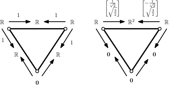
Figure 1: Two nonisomorphic sheaves with the same Laplacian.

3.2.1 Harmonic Cochains

The elements of $\ker\Delta^{k}=\mathcal{H}^{k}$ are known as harmonic $k$-cochains. More generally, a $k$-cochain may be harmonic on a subcomplex:

Definition 12.

A $k$-cochain $x$ of a sheaf $\mathcal{F}$ on a cell complex $X$ is harmonic on a set $S$ of $k$-cells if $(\Delta^{k}_{\mathcal{F}}x)|_{S}=0$.

When $k=0$ and $\mathcal{F}$ is the constant sheaf (i.e., in spectral graph theory), this can be expressed as a local averaging property: For each $v\in S$, $x_{v}=\frac{1}{d_{v}}\sum_{u\sim v}x_{u}$, where $\sim$ indicates adjacency and $d_{v}$ is the degree of the vertex $v$.

3.2.2 Identifying Sheaf Laplacians

Given a regular cell complex $X$ and a choice of dimension for each stalk, one can identify the collection of matrices which arise as coboundary maps for a sheaf on $X$ as those matrices satisfying a particular block sparsity pattern. This sparsity pattern controls the number of nonzero blocks in each row of the matrix. Restricting to $\delta^{0}$, we get a matrix whose rows have at most two nonzero blocks. The space of matrices which arise as sheaf Laplacians is then the space of matrices which have a factorization $L=\delta^{*}\delta$, where $\delta$ is a matrix satisfying this block sparsity condition. Boman et al. studied this class of matrices when the blocks have size $1\times 1$, calling them matrices of factor width two BCPT (05). They showed that this class coincides with the class of symmetric generalized diagonally dominant matrices, those matrices $L$ for which there exists a positive diagonal matrix $D$ such that $DLD$ is diagonally dominant. Indeed, the fact that sheaves on graphs are not in general determined by their Laplacians is in part a consequence of the nonuniqueness of width-two factorizations.

3.3 Approaching Infinite-Dimensional Laplacians

The definitions given in this paper are adapted to the case of sheaves of finite dimensional Hilbert spaces over finite cell complexes. Relaxing these finiteness constraints introduces new complications.

The spaces of cochains naturally acquire inner products by taking the Hilbert space direct sum. These are not the same as taking the algebraic direct sum or product of stalks. However, there is a sequence of inclusions of complexes

$$C^{\bullet}_{c}(X;\mathcal{F})\subseteq L^{2}C^{\bullet}(X;\mathcal{F})\subseteq C^{\bullet}(X;\mathcal{F})$$

inducing algebraic maps between the corresponding compactly supported, $L^{2}$, and standard sheaf cohomology theories.

The theory of abstract complexes of possibly infinite-dimensional Hilbert spaces has been developed in BL (92). This paper explains conditions for the spaces of harmonic cochains of a complex to be isomorphic with the algebraic cohomology of the complex. A particularly nice condition is that the complex have finitely generated cohomology, which implies that the total coboundary map is a Fredholm operator. More generally, if the images of the coboundary and its adjoint are closed, the spaces of harmonic cochains will be isomorphic to the cohomology.

Further issues arise when we consider the coboundary maps $\delta^{k}$. For spectral purposes, it is in general desirable for these to be bounded linear maps, for which we must make some further stipulations. Sufficient conditions for coboundary maps to be bounded are as follows:

Proposition 1.

Let $\mathcal{F}$ be a sheaf of Hilbert spaces on a cell complex $X$. Suppose that there exists some $M_{k}$ such that for every pair of cells $\sigma{\trianglelefteqslant}\tau$ with $\dim\sigma=k$ and $\dim\tau=k+1$, $\lVert\mathcal{F}_{\sigma{\trianglelefteqslant}\tau}\rVert\leq M_{k}$. Further suppose that every $k$-cell in $X$ has at most $d^{k}$ cofaces of dimension $k+1$, and every $(k+1)$-cell in $X$ has at most $d_{k+1}$ faces of dimension $k$. Then $\delta^{k}_{\mathcal{F}}$ is a bounded linear operator.

Proof.

We compute:

$$\lVert\delta^{k}x\rVert^{2}=\sum_{\dim\tau=k+1}\lVert(\delta^{k}x)_{\tau}\rVert^{2}\leq\sum_{\dim\tau=k+1}\left(\sum_{\sigma{\trianglelefteqslant}\tau}\lVert\mathcal{F}_{\sigma{\trianglelefteqslant}\tau}x_{\sigma}\rVert\right)^{2}\\ \leq\sum_{\dim\tau=k+1}\left(\sum_{\sigma{\trianglelefteqslant}\tau}M_{k}\lVert x_{\sigma}\rVert\right)^{2}\leq M_{k}^{2}\sum_{\dim\tau=k+1}d_{k+1}\sum_{\sigma{\trianglelefteqslant}\tau}\lVert x_{\sigma}\rVert^{2}\\ =M_{k}^{2}d_{k+1}\sum_{\dim\sigma=k}\sum_{\sigma{\trianglelefteqslant}\tau}\lVert x_{\sigma}\rVert^{2}\leq M_{k}^{2}d_{k+1}d^{k}\sum_{\dim\sigma=k}\lVert x_{\sigma}\rVert^{2}=M_{k}^{2}d_{k+1}d^{k}\lVert x\rVert^{2}.$$

∎

If $\delta^{k}$ is bounded, its associated Laplacians $\Delta^{k}_{+}=(\delta^{k})^{*}\delta^{k}$ and $\Delta^{k+1}_{-}=\delta^{k}(\delta^{k})^{*}$ are also bounded. As bounded self-adjoint operators, their spectral theory is relatively unproblematic. Their spectra consist entirely of approximate eigenvalues, those $\lambda$ for which there exists a sequence of unit vectors $\{x_{k}\}$ such that $\lVert\Delta^{k}_{+}x_{k}-\lambda x_{k}\rVert\to 0$.

If $\delta^{k}$ is not just bounded, but compact, the Laplacian spectral theory becomes even nicer. In this situation, the spectrum of $\Delta^{k}_{+}$ has no continuous part, and hence consists purely of eigenvalues. An appropriate decay condition on norms of restriction maps ensures compactness.

Proposition 2.

Let $\mathcal{F}$ be a sheaf of Hilbert spaces on a cell complex $X$. Suppose that for all $\sigma{\trianglelefteqslant}\tau$ with $\dim\sigma=k$ and $\dim\tau=k+1$, the restriction map $\mathcal{F}_{\sigma{\trianglelefteqslant}\tau}$ for is compact, and further that $\sum_{\sigma{\trianglelefteqslant}\tau}\lVert\mathcal{F}_{\sigma{\trianglelefteqslant}\tau}\rVert<\infty$. Then $\delta^{k}_{\mathcal{F}}$ is a compact linear operator.

Proof.

It is clear that $\delta^{k}$ cannot be compact if any one of its component restriction maps fails to be compact. Suppose first that all restriction maps are finite rank, and fix an ordering of $(k+1)$-cells of $X$, defining the orthogonal projection operators $P^{i}:C^{k+1}(X;\mathcal{F})\to C^{k+1}(X;\mathcal{F})$ sending stalks over $(k+1)$ cells of index greater than $i$ to zero. Then $P^{i}\delta^{k}$ is a finite-rank operator and

$$\lVert P^{i}\delta^{k}-\delta^{k}\rVert\leq\sum_{j>i}\sum_{\sigma{\trianglelefteqslant}\tau_{j}}\lVert\mathcal{F}_{\sigma{\trianglelefteqslant}\tau_{j}}\rVert,$$

which goes to zero as $i\to\infty$. In the case that the restriction maps are compact, pick an approximating sequence for each by finite rank maps and combine the two approximations. ∎

An important note is that when $C^{k}(X;\mathcal{F})$ is infinite dimensional and $\delta^{k}$ is compact with finite dimensional kernel, the eigenvalues of $\Delta^{k}_{+}$ will accumulate at zero. This means that there will be no smallest nontrivial eigenvalue for such Laplacians.

Most of the difficulties considered here already arise in the study of spectra of infinite graphs. The standard Laplacian associated to an infinite graph is bounded but not compact, while a proper choice of weights decaying at infinity makes it compact.

The study of sheaves of arbitrary Hilbert spaces on not-necessarily-finite cell complexes is interesting, and indeed suggests itself in certain applications. However, for the initial development and exposition of the theory, we have elected to focus on the (still quite interesting) finite-dimensional case. This is sufficient for most applications we have envisioned, and avoids the need for repeated qualifications and restrictions.

For the balance of this paper, we will assume that all cell complexes are finite and all vector spaces are finite dimensional, giving where possible proofs that generalize in some way to the infinite-dimensional setting. Most results that do not explicitly require a finite complex will extend quite directly to the case of sheaves with compact coboundary operators. Proofs not relying on the Courant-Fischer theorem will typically apply even to situations where coboundary operators are merely bounded, although their conclusions may be somewhat weakened.

3.4 The Normalized Laplacian and Weights

Many results in spectral graph theory rely on a normalized version of the standard graph Laplacian, which is typically defined in terms of a rescaling of the standard Laplacian. Let $D$ be the diagonal matrix whose nonzero entries are the degrees of vertices; then the normalized Laplacian is $\mathcal{L}=D^{-1/2}LD^{-1/2}$. This definition preserves the Laplacian as a symmetric matrix, but it obscures the true meaning of the normalization. The normalized Laplacian is the standard Laplacian with a different choice of weights for the vertices. The matrix $D^{-1/2}LD^{-1/2}$ is similar to $D^{-1}L$, which is self adjoint with respect to the inner product $\langle x,y\rangle=x^{T}Dy$. In this interpretation, each vertex is weighted proportionally to its degree. Viewing the normalization process as a reweighting of cells leads to the natural definition of normalized Laplacians for simplicial complexes given by Horak and Jost HJ (13).

Indeed, following Horak and Jost’s definition for simplicial complexes, we propose the following extension to sheaves.

Definition 13.

Let $\mathcal{F}$ be a weighted cellular sheaf defined on a regular cell complex $X$. We say $\mathcal{F}$ is normalized if for every cell $\sigma$ of $X$ and every $x,y\in\mathcal{F}(\sigma)\cap(\ker\delta)^{\perp}$, $\langle\delta x,\delta y\rangle=\langle x,y\rangle$.

Lemma 1.

Given a weighted sheaf $\mathcal{F}$ on a finite-dimensional cell complex $X$, it is always possible to reweight $\mathcal{F}$ to a normalized version.

Proof.

Note that if $X$ has dimension $k$, the normalization condition is trivially satisfied for all cells $\sigma$ of dimension $k$. Thus, starting at cells of dimension $k-1$, we recursively redefine the inner products on stalks. If $\sigma$ is a cell of dimension $k-1$, let $\Pi_{\sigma}$ be the orthogonal projection $\mathcal{F}(\sigma)\to\mathcal{F}(\sigma)\cap\ker\delta$. Then define the normalized inner product $\langle\bullet,\bullet\rangle^{N}_{\sigma}$ on $\mathcal{F}(\sigma)$ to be given by $\langle x,y\rangle^{N}_{\sigma}=\langle\delta(\operatorname{id}-\Pi_{\sigma})x,\delta(\operatorname{id}-\Pi_{\sigma})y\rangle+\langle\Pi_{\sigma}x,\Pi_{\sigma}y\rangle$. It is clear that this reweighted sheaf satisfies the condition of Definition 13 for cells of dimension $k$ and $k-1$. We may then perform this operation on cells of progressively lower dimension to obtain a fully normalized sheaf. ∎

Note that there is an important change of perspective here: we do not normalize the Laplacian of a sheaf, but instead normalize the sheaf itself, or more specifically, the inner products associated with each stalk of the sheaf.

If we apply this process to a sheaf $\mathcal{F}$ on a graph $G$, there is an immediate interpretation in terms of the original sheaf Laplacian. Let $D$ be the block diagonal of the standard degree 0 sheaf Laplacian, and note that for $x\perp\ker L$, $\langle x,Dx\rangle$ is the reweighted inner product on $C^{0}(G;\mathcal{F})$. In particular, the adjoint of $\delta$ with respect to this inner product has the form $D^{\dagger}\delta^{T}$, where $D^{\dagger}$ is the Moore-Penrose pseudoinverse of $D$, so that the matrix form of the reweighted Laplacian with respect to this inner product is $D^{\dagger}L$. Changing to the standard basis then gives $\mathcal{L}=D^{\dagger/2}LD^{\dagger/2}$.

3.5 Discrete Vector Bundles

A subclass of sheaves of particular interest are those where all restriction maps are invertible.These sheaves have been the subject of significantly more study than the general case, since they extend to locally constant sheaves on the geometric realization of the cell complex. The Riemann-Hilbert correspondence describes an equivalence between locally constant sheaves (or cosheaves) on $X$, local systems on $X$, vector bundles on $X$ with a flat connection, and representations of the fundamental groupoid of $X$. (See, e.g., (DK, 01, ch. 5) or ZS (09) for a discussion of some aspects of this correspondence.) When we represent a local system by a cellular sheaf or cosheaf, we will call it a discrete vector bundle.

One way to understand the space of $0$-cochains of a discrete vector bundle is as representing a subspace of the sections of a geometric realization of the associated flat vector bundle, defined by linear interpolation over higher-dimensional cells. The coboundary map can be seen as a sort of discretization of the connection, whose flatness is manifest in the fact that $\delta^{2}=0$.

Discrete vector bundles have some subtleties when we study their Laplacians. The sheaf-cosheaf duality corresponding to a local system, given by taking inverses of restriction maps, is not in general the same as the duality induced by an inner product on stalks. Indeed, these duals are only the same when the restriction maps are unitary — their adjoints must be their inverses.

The inner product on stalks of a cellular sheaf has two roles: it gives a relative weight to vectors in each stalk, but via the restriction maps also gives a relative weight to cells in the complex. This second role complicates our interpretation of certain sorts of vector bundles. For instance, one might wish to define an $O(n)$ discrete vector bundle on a graph to be a cellular sheaf of real vector spaces where all restriction maps are orthogonal. However, from the perspective of the degree-0 Laplacian, a uniform scaling of the inner product on an edge does not change the orthogonality of the bundle, but instead in some sense changes the length of the edge, or perhaps the degree of emphasis we give to discrepancies over that edge. So a discrete $O(n)$-bundle should be one where the restriction maps on each cell are scalar multiples of orthonormal maps.

That is, for each cell $\sigma$, we have a positive scalar $\alpha_{\sigma}$, such that for every $\sigma{\trianglelefteqslant}\tau$, the restriction map $\mathcal{F}_{\sigma{\trianglelefteqslant}\tau}$ is an orthonormal map times $\alpha_{\tau}/\alpha_{\sigma}$. One way to think of this is as a scaling of the inner product on each stalk of $\mathcal{F}$. Frequently, especially when dealing with graphs, we set $\alpha_{\sigma}=1$ when $\dim(\sigma)=0$, but this is not necessary. (Indeed, when dealing with the normalized Laplacian of a graph, we have $\alpha_{v}=\sqrt{d_{v}}$.)

The rationale for this particular definition is that in the absence of a basis, inner products are not absolutely defined, but only in relation to maps in or out of a space. Scaling the inner product on a vector space is meaningless except in relation to a given collection of maps, which it transforms in a uniform way.

As a special case of this definition, it will be useful to think about weighted versions of the constant sheaf. These are isomorphic to the ‘true’ constant sheaf, but not unitarily so. Weighted constant sheaves on a graph are analogous to weighted graphs. The distinction between the true constant sheaf and weighted versions arises because it is often convenient to think of the sections of a cellular sheaf as a subspace of $C^{0}(X;\mathcal{F})$. As a result, we often only want our sections to be constant on $0$-cells, allowing for variation up to a scalar multiple on higher-dimensional cells. This notion will be necessary in §8.6 when we discuss approximations of cellular sheaves.

3.6 Comparison with Previous Constructions

Friedman, in Fri (15), gave a definition of a sheaf on a graph, developed a homology theory, and suggested constructing sheaf Laplacians and adjacency matrices. The suggestion that one might develop a spectral theory of sheaves on graphs has remained until now merely a suggestion.

The graph connection Laplacian, introduced by Singer and Wu in SW (12), is simply the sheaf Laplacian of an $O(n)$-vector bundle over a graph. This construction has attracted significant interest from a spectral graph theory perspective, including the development of a Cheeger-type inequality BSS (13) and a study of random walks and sparsification CZ (12). Connection Laplacian methods have proven enlightening in the study of synchronization problems. Others have approached the study of vector bundles, and in particular line bundles, over graphs without reference to the connection Laplacian, studying analogues of spanning trees and the Kirchhoff theorems Ken (11); CCK (13). Other work on discrete approximations to connection Laplacians of manifolds has analyzed similar matrices Man (07).

Gao, Brodski, and Mukherjee developed a formulation in which the graph connection Laplacian is explicitly associated to a flat vector bundle on the graph and arises from a twisted coboundary operator GBM (16). This coboundary operator is not a sheaf coboundary map and has some difficulties in its definition. These arise from a lack of freedom to choose the basis for the space of sections over an edge of the graph. Further work by Gao uses a sheaf Laplacian-like construction to study noninvertible correspondences between probability distributions on surfaces Gao (16).

Wu et al. WRWX (18) have recently proposed a construction they call a weighted simplicial complex and studied its associated Laplacians. These are cellular cosheaves where all stalks are equal to a given vector space and restriction maps are scalar multiples of the identity. Their work discusses the cohomology and Hodge theory of weighted simplicial complexes, but did not touch on issues related to the Laplacian spectrum.

4 Harmonicity

As a prelude to results about the spectra of sheaf Laplacians, we will discuss issues related to harmonic cochains on sheaves. While these do not immediately touch on the spectral properties of the Laplacian, they are closely bound with its algebraic properties.

4.1 Harmonic Extension

Proposition 3.

Let $X$ be a regular cell complex with a weighted cellular sheaf $\mathcal{F}$. Let $B\subseteq X$ be a subcomplex and let $x|_{B}\in C^{k}(B;\mathcal{F})$ be an $\mathcal{F}$-valued $k$-cochain specified on $B$. If $H^{k}(X,B;\mathcal{F})=0$, then there exists a unique cochain $x\in C^{k}(X;\mathcal{F})$ which restricts to $x|_{B}$ on $B$ and is harmonic on $S=X\setminus B$.

Proof.

A matrix algebraic formulation suffices. Representing $\Delta^{k}_{\mathcal{F}}$ in block form as partitioned by $B$ and $S$, the relevant equation is

$$\begin{bmatrix}\Delta^{k}_{\mathcal{F}}(S,S)&\Delta^{k}_{\mathcal{F}}(S,B)\\ \Delta^{k}_{\mathcal{F}}(B,S)&\Delta^{k}_{\mathcal{F}}(B,B)\end{bmatrix}\begin{bmatrix}x|_{S}\\ x|_{B}\end{bmatrix}=\begin{bmatrix}0\\ y\end{bmatrix}.$$

Since $y$ is indeterminate, we can ignore the second row of the matrix, giving the equation $\Delta^{k}_{\mathcal{F}}(S,S)x|_{S}+\Delta^{k}_{\mathcal{F}}(S,B)x|_{B}=0$. We can write $\Delta_{\mathcal{F}}^{k}(S,S)=(\delta^{k}|_{S})^{*}\delta^{k}|_{S}+((\delta^{k-1})^{*}|_{S})^{*}(\delta^{k-1})^{*}|_{S}$, which is very close to the $k$-th Hodge Laplacian of the relative cochain complex

$$\cdots\to C^{k-1}(X,B;\mathcal{F})\to C^{k}(X,B;\mathcal{F})\to C^{k+1}(X,B;\mathcal{F})\to\cdots.$$

Indeed, we can exploit the fact that this is a subcomplex of $C^{\bullet}(X;\mathcal{F})$ to compute its Hodge Laplacian in terms of the coboundary maps of $C^{\bullet}(X;\mathcal{F})$. The coboundary map $\delta_{S}$ of $C^{\bullet}(X,B;\mathcal{F})$ is simply the restriction of the coboundary map $\delta$ of $C^{\bullet}(X;\mathcal{F})$ to the subcomplex: $\delta_{S}^{k}=\pi_{S}^{k+1}\delta^{k}i_{S}^{k}$, where $\pi_{S}^{k}$ is the orthogonal projection $C^{k}(X;\mathcal{F})\to C^{k}(X,B;\mathcal{F})$ and $i_{S}^{k}$ the inclusion $C^{k}(X,B;\mathcal{F})\to C^{k}(X;\mathcal{F})$. Note that $\pi_{S}^{k}$ and $i_{S}^{k}$ are adjoints, and that $i_{S}^{k}\pi_{S}^{k}$ is the identity on $\operatorname{im}\delta^{k-1}_{S}$. We may therefore write the Hodge Laplacian of the relative complex as

$$\Delta^{k}(X,B;\mathcal{F})=(\delta^{k}_{S})^{*}\delta^{k}_{S}+\delta^{k-1}_{S}(\delta^{k-1}_{S})^{*}\\ =\pi_{S}^{k}(\delta^{k})^{*}i_{S}^{k+1}\pi_{S}^{k+1}\delta^{k}i_{S}^{k}+\pi_{S}^{k}\delta^{k-1}i_{S}^{k-1}\pi_{S}^{k-1}(\delta^{k-1})^{*}i_{S}^{k}\\ =\pi_{S}^{k}(\delta^{k})^{*}\delta^{k}i_{S}^{k}+\pi_{S}^{k}\delta^{k-1}i_{S}^{k-1}\pi_{S}^{k-1}(\delta^{k-1})^{*}i_{S}^{k}.$$

Meanwhile, we can write the submatrix

$$\Delta_{\mathcal{F}}^{k}(S,S)=\pi_{S}^{k}(\delta^{k})^{*}\delta^{k}i_{S}^{k}+\pi_{S}^{k}\delta^{k-1}(\delta^{k-1})^{*}i_{S}^{k}.$$

It is then immediate that $\ker(\Delta_{\mathcal{F}}^{k}(S,S))\subseteq\ker\Delta^{k}(X,B;\mathcal{F})$, so that $\Delta_{\mathcal{F}}^{k}(S,S)$ is invertible if $H^{k}(X,B;\mathcal{F})=0$. ∎

If we restrict to up- or down-Laplacians, a harmonic extension always exists, even if it is not unique. This is because, for instance, $\operatorname{im}(\delta^{k}|_{S})^{*}\delta^{k}|_{B}\subseteq\operatorname{im}(\delta^{k}|_{S})^{*}\delta^{k}|_{S}$. In particular, this implies that harmonic extension is always possible for $0$-cochains, with uniqueness if and only if $H^{0}(X,B;\mathcal{F})=0$.

4.2 Kron Reduction

Kron reduction is one of many names given to a process of simplifying graphs with respect to the properties of their Laplacian on a boundary. If $G$ is a connected graph with a distinguished set of vertices $B$, which we consider as a sort of boundary of $G$, Proposition 3 shows that there is a harmonic extension map $E:\mathbb{R}^{B}\to\mathbb{R}^{V(G)}$. It is then possible to construct a graph $G^{\prime}$ on $B$ such that for every function $x$ on the vertices of $G^{\prime}$, we have $L_{G^{\prime}}x=\pi_{B}L_{G}E(x)$, where $\pi_{B}$ is the orthogonal projection map $\mathbb{R}^{V(G)}\to\mathbb{R}^{B}$. Indeed, letting $S=V(G)\setminus B$, we have $E(x)|_{S}=-L_{G}(S,S)^{-1}L_{G}(S,B)x$, so

$$L_{G^{\prime}}x=\pi_{B}L_{G}E(x)=L_{G}(B,B)x-L_{G}(B,S)L_{G}(S,S)^{-1}L_{G}(S,B)x.$$

Therefore,

$$L_{G^{\prime}}=L_{G}(B,B)-L_{G}(B,S)L_{G}(S,S)^{-1}L_{G}(S,B),$$

that is, $L_{G^{\prime}}$ is the Schur complement of the $(B,B)$ block of $L_{G}$. It is also the Laplacian of a graph on $B$:

Theorem 4.1 (see DB (13)).

If $L_{G}$ is the Laplacian of a connected graph $G$, and $B$ a subset of vertices of $G$, then $L_{G^{\prime}}=L_{G}(B,B)-L_{G}(B,S)L_{G}(S,S)^{-1}L_{G}(S,B)$ is the Laplacian of a graph with vertex set $B$.

A physically-inspired way to understand this result (and a major use of Kron reduction in practice) is to view it as reducing a network of resistors given by $G$ to a smaller network with node set $B$ that has the same electrical behavior on $B$ as the original network. In this guise, Kron reduction is a high-powered version of the $Y$-$\Delta$ and star-mesh transforms familiar from circuit analysis. Further discussion of Kron reduction and its various implications and applications may be found in DB (13).

Can we perform Kron reduction on sheaves? That is, given a sheaf $\mathcal{F}$ on a graph $G$ with a prescribed boundary $B$, can we find a sheaf $\mathcal{F}_{B}$ on a graph with vertex set $B$ only such that for every $x\in C^{0}(B;\mathcal{F}_{B})$ we have $L_{\mathcal{F}_{B}}x=\pi_{C^{0}(B;\mathcal{F}_{B})}L_{\mathcal{F}}E(x)$, where $E(x)$ is the harmonic extension of $x$ to $G$?

The answer is, in general, no. Suppose we want to remove the vertex $v$ from our graph, i.e., $B=G\setminus\{v\}$. Let $D_{v}=\sum_{v{\trianglelefteqslant}e}\mathcal{F}_{v{\trianglelefteqslant}e}^{*}\mathcal{F}_{v{\trianglelefteqslant}e}=L_{v,v}$. To eliminate the vertex $v$ we apply the condition $(L_{\mathcal{F}}(x,E(x)))(v)=0$, and take a Schur complement, replacing $L(B,B)$ with $L(B,B)-L(B,v)D_{v}^{-1}L(v,B)$. This means that we add to the entry $L(w,w^{\prime})$ the map $\mathcal{F}_{w{\trianglelefteqslant}e}^{*}\mathcal{F}_{v{\trianglelefteqslant}e}D_{v}^{-1}\mathcal{F}_{v{\trianglelefteqslant}e^{\prime}}^{*}\mathcal{F}_{w^{\prime}{\trianglelefteqslant}e^{\prime}}$, where $e$ is the edge between $v$ and $w$, and $e^{\prime}$ the edge between $v$ and $w^{\prime}$. This does not in general translate to a change in the restriction maps for the edge between $w$ and $w^{\prime}$. In general, Kron reduction is not possible for sheaves.

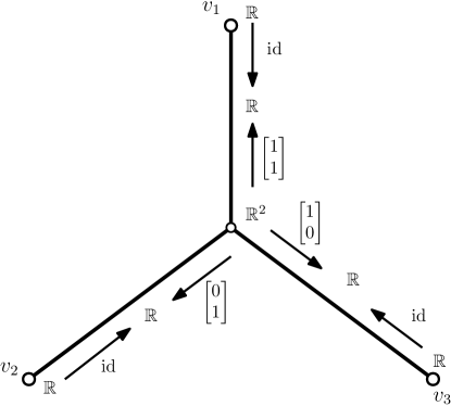
Figure 2: A sheaf illustrating the general impossibility of Kron reduction.

In particular, if $x\in C^{0}(G;\mathcal{F})$ is a section of $\mathcal{F}$, its restriction to $B$ must be a section of $\mathcal{F}_{B}$. Conversely, if $x$ is not a section, its restriction to $B$ cannot be a section of $\mathcal{F}_{B}$. But we can construct sheaves with a space of sections on the boundary that cannot be replicated with a sheaf on the boundary vertices only. For instance, take the star graph with three boundary vertices, with stalks $\mathbb{R}$ over boundary vertices and edges, and $\mathbb{R}^{2}$ over the internal vertex. Take as the restriction maps from the central vertex restriction onto the first and second components, and addition of the two components. See Figure 2 for an illustration.

Note that a global section of this sheaf is determined by its value on the central vertex. If we label the boundary vertices counterclockwise starting at the top, the space of global sections for $\mathcal{F}_{B}$ must have as a basis

$$x_{1}=\begin{bmatrix}1\\ 1\\ 0\end{bmatrix},\quad x_{2}=\begin{bmatrix}1\\ 0\\ 1\end{bmatrix}.$$

But there is no sheaf on a graph with vertex set $B$ which has this space of global sections. To see this, note that if $x_{1}$ is a section, the map from $\mathcal{F}(v_{1})$ to $\mathcal{F}(v_{3})$ must be the zero map, and similarly for the map from $\mathcal{F}(v_{2})$ to $\mathcal{F}(v_{3})$. Similarly, if $x_{2}$ is a section, the maps $\mathcal{F}(v_{1})\to\mathcal{F}(v_{2})$ and $\mathcal{F}(v_{3})\to\mathcal{F}(v_{2})$ must be zero. But this already shows that the vector $\begin{bmatrix}1&0&0\end{bmatrix}^{T}$ must be a section, giving $\mathcal{F}_{B}$ a three-dimensional space of sections. The problem is that the internal node allows for constraints between boundary nodes that cannot be expressed by purely pairwise interactions. This fact is a fundamental obstruction to Kron reduction for general sheaves.

However, there is a sheaf Kron reduction for sheaves with vertex stalks of dimension at most 1. This follows from the identification of the Laplacians of such sheaves as the matrices of factor width two in §3.2.2.

Theorem 4.2.

The class of matrices of factor width at most two is closed under taking Schur complements.

Proof.

By Theorems 8 and 9 of BCPT (05), a matrix $L$ has factor width at most two if and only if it is symmetric and generalized weakly diagonally dominant with nonnegative diagonal, that is, there exists a positive diagonal matrix $D$ such that $DLD$ is weakly diagonally dominant. Equivalently, these are the symmetric positive semidefinite generalized weakly diagonally dominant matrices. The class of generalized weakly diagonally dominant matrices coincides with the class of $H$-matrices, which are shown to be closed under Schur complements in JS (05). Similarly, the class of symmetric positive definite matrices is closed under Schur complements, so the intersection of the two classes is also closed. ∎

4.3 Maximum Modulus Theorem

Harmonic $0$-cochains of an $O(n)$-bundle satisfy a local averaging property which leads directly to a maximum modulus principle.

Lemma 2.

Let $G$ be a graph with an $O(n)$-bundle $\mathcal{F}$, with constant vertex weights $\alpha_{v}=1$ and arbitrary edge weights $\alpha_{e}$ (as defined in §3.5). If $x\in C^{0}(G;\mathcal{F})$ is harmonic at a vertex $v$, then

$$x_{v}=\frac{1}{d_{v}}\sum_{\begin{subarray}{c}v,w{\trianglelefteqslant}e\\ v\neq w\end{subarray}}\mathcal{F}_{v{\trianglelefteqslant}e}^{*}\mathcal{F}_{w{\trianglelefteqslant}e}x_{w},$$

where $d_{v}=\sum_{v{\trianglelefteqslant}e}\lVert\mathcal{F}_{v{\trianglelefteqslant}e}\rVert^{2}=\sum_{v{\trianglelefteqslant}e}\alpha_{e}^{2}$.

Proof.

The block row of $L_{\mathcal{F}}$ corresponding to $v$ has entries $-\mathcal{F}_{v{\trianglelefteqslant}e}^{*}\mathcal{F}_{w{\trianglelefteqslant}e}$ off the diagonal and $\sum_{v{\trianglelefteqslant}e}\mathcal{F}_{v{\trianglelefteqslant}e}^{*}\mathcal{F}_{v{\trianglelefteqslant}e}=\sum_{v{\trianglelefteqslant}e}\lVert\mathcal{F}_{v{\trianglelefteqslant}e}\rVert^{2}\operatorname{id}_{\mathcal{F}(v)}$ on the diagonal. The harmonicity condition is then

$$d_{v}x_{v}-\sum_{\begin{subarray}{c}v,w{\trianglelefteqslant}e\\ v\neq w\end{subarray}}\mathcal{F}_{v{\trianglelefteqslant}e}^{*}\mathcal{F}_{w{\trianglelefteqslant}e}x_{w}=0.$$

∎

Theorem 4.3 (Maximum modulus principle).

Let $G$ be a graph, and $B$ be a thin subset of vertices of $G$; that is, $G\setminus B$ is connected, and every vertex in $B$ is connected to a vertex not in $B$. Let $\mathcal{F}$ be an $O(n)$-bundle on $G$ with $a_{v}=1$ for all $v\in G$, and suppose $x\in C^{0}(G;\mathcal{F})$ is harmonic on $G\setminus B$. Then if $x$ attains its maximum stalkwise norm at a vertex in $G\setminus B$, it has constant stalkwise norm.

Proof.

Note that for a given edge $e=v\sim w$, $\mathcal{F}_{v{\trianglelefteqslant}e}$ and $\mathcal{F}_{u{\trianglelefteqslant}e}$ are both $\alpha_{e}$ times an orthogonal map, so $\mathcal{F}_{v{\trianglelefteqslant}e}^{*}\mathcal{F}_{w{\trianglelefteqslant}e}$ is $\alpha_{e}^{2}$ times an orthogonal map. Let $v\in G\setminus B$ and suppose $\lVert x_{v}\rVert\geq\lVert x_{w}\rVert$ for all $w\in G$. Then this holds in particular for neighbors of $v$, so that we have

$$\lVert x_{v}\rVert=\frac{1}{d_{v}}\lVert\sum_{\begin{subarray}{c}v,w{\trianglelefteqslant}e\\ v\neq w\end{subarray}}\mathcal{F}_{v{\trianglelefteqslant}e}^{*}\mathcal{F}_{w{\trianglelefteqslant}e}x_{w}\rVert\leq\frac{1}{d_{v}}\sum_{\begin{subarray}{c}v,w{\trianglelefteqslant}e\\ v\neq w\end{subarray}}\lVert\mathcal{F}_{v{\trianglelefteqslant}e}^{*}\mathcal{F}_{w{\trianglelefteqslant}e}x_{w}\rVert\\ =\frac{1}{d_{v}}\sum_{\begin{subarray}{c}v,w{\trianglelefteqslant}e\\ v\neq w\end{subarray}}\alpha_{e}^{2}\lVert x_{w}\rVert\leq\frac{1}{d_{v}}\sum_{v{\trianglelefteqslant}e}\alpha_{e}^{2}\lVert x_{v}\rVert=\lVert x_{v}\rVert,$$

Equality holds throughout, which, combined with the assumption that $\lVert x_{v}\rVert\geq\lVert x_{w}\rVert$ for all $w$, forces $\lVert x_{v}\rVert=\lVert x_{w}\rVert$ for $w\sim v$. We then apply the same argument to every vertex in $G\setminus B$ adjacent to $v$, and, after iterating, the region of constant stalkwise norm extends to all of $G\setminus B$ because this subgraph is connected. But since every vertex $b\in B$ is adjacent to some vertex $w\in G\setminus B$, the same argument applied to the neighborhood of $w$ forces $\lVert x_{b}\rVert=\lVert x_{w}\rVert$. So any harmonic function that attains its maximum modulus on $G\setminus B$ has constant modulus. ∎

Corollary 1.

Let $B$ be a thin subset of vertices of $G$, and $\mathcal{F}$ an $O(n)$-bundle on $G$ as before. If $x\in C^{0}(G;\mathcal{F})$ is harmonic on $G\setminus B$, then it attains its maximum modulus on $B$.

The constant sheaf on a graph is an $O(n)$-bundle, so this result gives a maximum modulus principle for harmonic functions on the vertices of a graph. A slightly stronger result in this vein, involving maxima and minima of $x$, is discussed in Sun (08). The thinness condition for $B$ is not strictly necessary for the corollary to hold — there are a number of potential weakenings of the condition. For instance, we might simply require that there exists some $w\in B$ such that for every vertex $v\in G\setminus B$ there exists a path from $v$ to $w$ not passing through $B$.

5 Spectra of Sheaf Laplacians

The results in this section are straightforward generalizations and extensions of familiar results from spectral graph theory. Most are not particularly difficult, but they illustrate the potential for lifting nontrivial notions from graphs and complexes to sheaves.

It is useful to note a few basic facts about the spectra of Laplacians arising from Hodge theory.

Proposition 4.

The nonzero spectrum of $\Delta^{k}$ is the disjoint union of the nonzero spectra of $\Delta^{k}_{+}$ and $\Delta^{k}_{-}$.

Proof.

We take advantage of the Hodge decomposition, noting that $C^{k}(X;\mathcal{F})=\ker\Delta^{k}\oplus\operatorname{im}\Delta^{k}_{-}\oplus\operatorname{im}\Delta^{k}_{+}$. This is an orthogonal decomposition, and $=0$ as well as $\Delta^{k}_{-}|_{(\operatorname{im}\Delta^{k}_{+})}=0$. Further, since $\ker\Delta^{k}=\ker\Delta_{+}\cap\ker\Delta_{-}$, both restrict to zero on the kernel of $\Delta^{k}$. We therefore see that $\Delta^{k}$ is the orthogonal direct sum $0|_{\ker\Delta^{k}}\oplus\Delta^{k}_{+}|_{(\operatorname{im}\Delta^{k}_{+})}\oplus\Delta^{k}_{-}|_{(\operatorname{im}\Delta^{k}_{-})}$, and hence the spectrum of $\Delta^{k}$ is the union of the spectra of these three operators. ∎

Proposition 5.

The nonzero eigenvalues of $\Delta^{k}_{+}$ and $\Delta^{k+1}_{-}$ are the same.

Proof.

We have $\Delta^{k}_{+}=(\delta^{k})^{*}\delta^{k}$ and $\Delta^{k+1}_{-}=\delta^{k}(\delta^{k})^{*}$. The eigendecompositions of these matrices are determined by the singular value decomposition of $\delta^{k}$, and the nonzero eigenvalues are precisely the squares of the nonzero singular values of $\delta^{k}$.

∎

One reason for the study of the normalized graph Laplacian is that its spectrum is bounded above by 2 Chu (92), and hence normalized Laplacian spectra of different graphs can be easily compared. A similar result holds for up-Laplacians of normalized simplicial complexes HJ (13): the eigenvalues of the degree-$k$ up-Laplacian of a normalized simplicial complex are bounded above by $k+2$. This fact extends to normalized sheaves on simplicial complexes. This result and others in this paper will rely on the Courant-Fischer theorem, which we state here for reference.

Definition 14.

Let $A$ be a self-adjoint operator on a Hilbert space ${\mathbb{V}}$. If $x\in{\mathbb{V}}$, the Rayleigh quotient corresponding to $x$ and $A$ is

$$R_{A}(x)=\frac{\langle x,Ax\rangle}{\langle x,x\rangle}.$$

Theorem 5.1 (Courant-Fischer).

Let $A$ be an $n\times n$ Hermitian matrix with eigenvalues $\lambda_{1}\leq\lambda_{2}\leq\cdots\leq\lambda_{n}$. Then

$$\lambda_{k}=\min_{\dim V=k}\max_{x\in V}R_{A}(x)=\max_{\dim V=n-k+1}\min_{x\in V}R_{A}(x).$$

The proof is immediate once one uses the fact that $A$ is unitarily equivalent to a diagonal matrix.

Proposition 6.

Suppose $\mathcal{F}$ is a normalized sheaf on a simplicial complex $X$. The eigenvalues of the degree $k$ up-Laplacian $L^{k}_{\mathcal{F}}$ are bounded above by $k+2$.

Proof.

By the Courant-Fischer theorem, the largest eigenvalue of $L^{k}_{\mathcal{F}}$ is equal to

$$\max_{x\in C^{k}(X;\mathcal{F})}\frac{\langle x,L^{k}_{\mathcal{F}}x\rangle}{\langle x,x\rangle}=\max_{x\perp\ker\delta^{k}}\frac{\langle\delta^{k}x,\delta^{k}x\rangle}{\sum\limits_{\dim\sigma=k}\langle\delta^{k}x_{\sigma},\delta^{k}x_{\sigma}\rangle}\\ =\max_{x\perp\ker\delta^{k}}\frac{\sum\limits_{\dim\tau=k+1}\sum\limits_{\sigma,\sigma^{\prime}{\trianglelefteqslant}\tau}[\sigma:\tau][\sigma^{\prime}:\tau]\langle\mathcal{F}_{\sigma{\trianglelefteqslant}\tau}x_{\sigma},\mathcal{F}_{\sigma^{\prime}{\trianglelefteqslant}\tau}x_{\sigma^{\prime}}\rangle}{\sum\limits_{\dim\sigma=k}\sum\limits_{\sigma{\trianglelefteqslant}\tau}\langle\mathcal{F}_{\sigma{\trianglelefteqslant}\tau}x_{\sigma},\mathcal{F}_{\sigma{\trianglelefteqslant}\tau}x_{\sigma}\rangle}.$$

Note that for $\sigma\neq\sigma^{\prime}$,

$$[\sigma:\tau][\sigma^{\prime}:\tau]\langle\mathcal{F}_{\sigma{\trianglelefteqslant}\tau}x_{\sigma},\mathcal{F}_{\sigma^{\prime}{\trianglelefteqslant}\tau}x_{\sigma^{\prime}}\rangle\leq\lVert\mathcal{F}_{\sigma{\trianglelefteqslant}\tau}x_{\sigma}\rVert\lVert\mathcal{F}_{\sigma^{\prime}{\trianglelefteqslant}\tau}x_{\sigma^{\prime}}\rVert\\ \leq\frac{1}{2}\left(\lVert\mathcal{F}_{\sigma{\trianglelefteqslant}\tau}x_{\sigma}\rVert^{2}+\lVert\mathcal{F}_{\sigma^{\prime}{\trianglelefteqslant}\tau}x_{\sigma^{\prime}}\rVert^{2}\right)$$

by the Cauchy-Schwarz inequality. In particular, then, the term of the numerator corresponding to each $\tau$ of dimension $k+1$ is bounded above by

$$\sum_{\sigma{\trianglelefteqslant}\tau}\lVert\mathcal{F}_{\sigma{\trianglelefteqslant}\tau}x_{\sigma}\rVert^{2}+\frac{1}{2}\sum_{\sigma\neq\sigma^{\prime}{\trianglelefteqslant}\tau}\left(\lVert\mathcal{F}_{\sigma{\trianglelefteqslant}\tau}x_{\sigma}\rVert^{2}+\lVert\mathcal{F}_{\sigma^{\prime}{\trianglelefteqslant}\tau}x_{\sigma^{\prime}}\rVert^{2}\right)=(k+2)\sum_{\sigma{\trianglelefteqslant}\tau}\lVert\mathcal{F}_{\sigma{\trianglelefteqslant}\tau}x_{\sigma}\rVert^{2},$$

by counting the number of times each term $\lVert\mathcal{F}_{\sigma{\trianglelefteqslant}\tau}x_{\sigma}\rVert^{2}$ appears in the sum. Meanwhile, the denominator is equal to $\displaystyle\sum_{\dim\tau=k+1}\sum_{\sigma{\trianglelefteqslant}\tau}\lVert\mathcal{F}_{\sigma{\trianglelefteqslant}\tau}x_{\sigma}\rVert^{2}$, so the Rayleigh quotient is bounded above by $k+2$. ∎

5.1 Eigenvalue Interlacing

Definition 15.

Let $A$, $B$ be $n\times n$ matrices with real spectra. Let $\lambda_{1}\leq\lambda_{2}\leq\cdots\leq\lambda_{n}$ be the eigenvalues of $A$ and $\mu_{1}\leq\mu_{2}\leq\cdots\leq\mu_{n}$ be the eigenvalues of $B$. We say the eigenvalues of $A$ are $\mathbf{(p,q)}$-interlaced with the eigenvalues of $B$ if for all $k$, $\lambda_{k-p}\leq\mu_{k}\leq\lambda_{k+q}$. (We let $\lambda_{k}=\lambda_{1}$ for $k<1$ and $\lambda_{k}=\lambda_{n}$ for $k>n$.)

The eigenvalues of low-rank perturbations of symmetric positive semidefinite matrices are related by interlacing. The following is a standard result:

Theorem 5.2.

Let $A$ and $B$ be positive semidefinite matrices, with $\operatorname{rank}B=t$. Then the eigenvalues of $A$ are $(t,0)$-interlaced with the eigenvalues of $A-B$.

Proof.

Let $\mu_{k}$ be the $k$-th largest eigenvalue of $A-B$ and $\lambda_{k}$ the $k$-th largest eigenvalue of $A$. By the Courant-Fischer theorem, we have

$$\mu_{k} =\min_{\dim Y=k}\left(\max_{y\in Y,y\neq 0}\frac{\langle y,Ay\rangle-\langle y,By\rangle}{\langle y,y\rangle}\right)$$

$$\geq\min_{\dim Y=k}\left(\max_{y\in Y\cap\ker B,y\neq 0}\frac{\langle y,Ay\rangle}{\langle y,y\rangle}\right)$$

$$\geq\min_{\dim Y=k-t}\left(\max_{y\in Y,y\neq 0}\frac{\langle y,Ay\rangle}{\langle y,y\rangle}\right)=\lambda_{k-t}$$

and

$$\lambda_{k} =\min_{\dim Y=k}\left(\max_{y\in Y,y\neq 0}\frac{\langle y,Ay\rangle}{\langle y,y\rangle}\right)$$

$$\geq\min_{\dim Y=k}\left(\max_{y\in Y,y\neq 0}\frac{\langle y,Ay\rangle-\langle y,By\rangle}{\langle y,y\rangle}\right)=\mu_{k}.$$

∎

This result is immediately applicable to the spectra of sheaf Laplacians under the deletion of cells from their underlying complexes. The key part is the interpretation of the difference of the two Laplacians as the Laplacian of a third sheaf. Let $\mathcal{F}$ be a sheaf on $X$, and let $C$ be an upward-closed set of cells of $X$, with $Y=X\setminus C$. The inclusion map $i:Y\to X$ induces a restriction of $\mathcal{F}$ onto $Y$, the pullback sheaf $i^{*}\mathcal{F}$. Consider the Hodge Laplacians $\Delta^{k}_{\mathcal{F}}$ and $\Delta^{k}_{i^{*}\mathcal{F}}$. If $C$ contains cells of dimension $k$, these matrices are different sizes, but we can derive a relationship by padding $\Delta^{k}_{i^{*}\mathcal{F}}$ with zeroes. Equivalently, this is the degree-$k$ Laplacian of $\mathcal{F}$ with the restriction maps incident to cells in $C$ set to zero.

Proposition 7.

Let $\mathcal{G}$ be the sheaf on $X$ with the same stalks as $\mathcal{F}$ but with all restriction maps between cells not in $C$ set to zero. The eigenvalues of $\Delta^{k}_{i^{*}\mathcal{F}}$ are $(t,0)$-interlaced with the eigenvalues of $\Delta^{k}_{\mathcal{F}}$, where $t=\operatorname{codim}H^{k}(X;\mathcal{G})=\dim C^{k}(X;\mathcal{F})-\dim H^{k}(X;\mathcal{G})$.

Similar results can be derived for the up- and down-Laplacians. Specializing to graphs, interlacing is also possible for the normalized degree 0 sheaf Laplacian. The Rayleigh quotient for the normalized Laplacian $\mathcal{L}_{i^{*}\mathcal{F}}$ is

$$\frac{\langle x,D_{i^{*}\mathcal{F}}^{-1/2}L_{i^{*}\mathcal{F}}D_{i^{*}\mathcal{F}}^{-1/2}x\rangle}{\langle x,x\rangle}=\frac{\langle y,L_{i^{*}\mathcal{F}}y\rangle}{\langle y,D_{i^{*}\mathcal{F}}y\rangle}=\frac{\langle y,L_{\mathcal{F}}y\rangle-\langle y,L_{\mathcal{G}}y\rangle}{\langle y,D_{\mathcal{F}}y\rangle-\langle y,D_{\mathcal{G}}y\rangle},$$

where we let $y=D_{i^{*}\mathcal{F}}^{-1/2}x$. Then if $\{\lambda_{k}\}$ are the ordered eigenvalues of $\mathcal{L}_{\mathcal{F}}$ and $\{\mu_{k}\}$ are the ordered eigenvalues of $\mathcal{L}_{i^{*}\mathcal{F}}$, we have

$$\mu_{k} =\min_{\dim Y=k}\left(\max_{y\in Y,y\neq 0}\frac{\langle y,L_{\mathcal{F}}y\rangle-\langle y,L_{\mathcal{G}}y\rangle}{\langle y,D_{\mathcal{F}}y\rangle-\langle y,D_{\mathcal{G}}y\rangle}\right)$$

$$\geq\min_{\dim Y=k}\left(\max_{y\in Y\cap H^{0}(X;\mathcal{G}),y\neq 0}\frac{\langle y,L_{\mathcal{F}}y\rangle}{\langle y,D_{\mathcal{F}}y\rangle-\langle y,D_{\mathcal{G}}y\rangle}\right)$$

$$\geq\min_{\dim Y=k}\left(\max_{y\in Y\cap H^{0}(X;\mathcal{G}),y\neq 0}\frac{\langle y,L_{\mathcal{F}}y\rangle}{\langle y,D_{\mathcal{F}}y\rangle}\right)$$

$$\geq\min_{\dim Y=k-t}\left(\max_{y\in Y,y\neq 0}\frac{\langle y,L_{\mathcal{F}}y\rangle}{\langle y,D_{\mathcal{F}}y\rangle}\right)=\lambda_{k-t}$$

$$\mu_{k} =\max_{\dim Y=n-k+1}\left(\min_{y\in Y,y\neq 0}\frac{\langle y,L_{\mathcal{F}}y\rangle-\langle y,L_{\mathcal{G}}y\rangle}{\langle y,D_{\mathcal{F}}y\rangle-\langle y,D_{\mathcal{G}}y\rangle}\right)$$

$$\leq\max_{\dim Y=n-k+1}\left(\min_{y\in Y\cap H^{0}(X;\mathcal{G}),y\neq 0}\frac{\langle y,L_{\mathcal{F}}y\rangle}{\langle y,D_{\mathcal{F}}y\rangle-\langle y,D_{\mathcal{G}}y\rangle}\right)$$

$$\leq\max_{\dim Y=n-k+1}\left(\min_{y\in Y\cap H^{0}(X;\mathcal{G}),y\neq 0}\frac{\langle y,L_{\mathcal{F}}y\rangle}{\langle y,D_{\mathcal{F}}y\rangle}\right)$$

$$\leq\max_{\dim Y=n-k-t+1}\left(\min_{y\in Y,y\neq 0}\frac{\langle y,L_{\mathcal{F}}y\rangle}{\langle y,D_{\mathcal{F}}y\rangle}\right)=\lambda_{k+t}$$

Therefore, the eigenvalues of the normalized Laplacians are $(t,t)$-interlaced. This generalizes interlacing results for normalized graph Laplacians.

5.2 Sheaf Morphisms

Proposition 8.

Suppose $\varphi:\mathcal{F}\to\mathcal{G}$ is a morphism of weighted sheaves on a regular cell complex $X$. If $\varphi^{k+1}$ is a unitary map, then $L^{k}_{\mathcal{F}}=(\varphi^{k})^{*}L^{k}_{\mathcal{G}}\varphi^{k}$.

Proof.

The commutativity condition $\varphi^{k+1}\delta^{\mathcal{F}}=\delta^{\mathcal{G}}\varphi^{k}$ implies that $(\delta^{\mathcal{F}})^{*}(\varphi^{k+1})^{*}\varphi^{k+1}\delta^{\mathcal{F}}=(\varphi^{k})^{*}(\delta^{\mathcal{G}})^{*}\delta^{\mathcal{G}}\varphi^{k}=(\varphi^{k})^{*}L^{k}_{\mathcal{G}}\varphi^{k}$. Thus if $(\varphi^{k+1})^{*}\varphi^{k+1}=\operatorname{id}_{C^{k+1}(X;\mathcal{F})}$, we have $L^{k}_{\mathcal{F}}=(\varphi^{k})^{*}L^{k}_{\mathcal{G}}\varphi^{k}$. This condition holds if $\varphi^{k+1}$ is unitary. ∎

An analogous result holds for the down-Laplacians of $\mathcal{F}$, and these combine to a result for the full Hodge Laplacians.

5.3 Cell Complex Morphisms

The following constructions are restricted to locally injective cellular morphisms, as discussed in §2.1. Recall that under these morphisms, cells map to cells of the same dimension and the preimage of the star of a cell is a disjoint union of subcomplexes, on each of which the map acts injectively. The sheaf Laplacian is invariant with respect to pushforwards over such maps:

Proposition 9.

Let $X$ and $Y$ be cell complexes, and let $f:X\to Y$ be a locally injective cellular morphism. If $\mathcal{F}$ is a sheaf on $X$, the $k$th coboundary Laplacian corresponding to $f_{*}\mathcal{F}$ on $Y$ is the same (up to a unitary change of basis) as the $k$th coboundary Laplacian of $\mathcal{F}$ on $X$.

Corollary 2.

The sheaves $\mathcal{F}$ and $f_{*}\mathcal{F}$ are isospectral for the coboundary Laplacian.

Proof.

There is a canonical isometry $f_{k}:C^{k}(X,\mathcal{F})\to C^{k}(Y,f_{*}\mathcal{F})$, which is given on stalks by the obvious inclusion $f_{\sigma}:\mathcal{F}(\sigma)\to f_{*}\mathcal{F}(f(\sigma))=\bigoplus_{f(\tau)=f(\sigma)}\mathcal{F}(\tau)$. For $\sigma{\trianglelefteqslant}\sigma^{\prime}$, $f_{\sigma}$ commutes with the restriction map $\mathcal{F}_{\sigma{\trianglelefteqslant}\sigma^{\prime}}$ and hence $f_{k}$ commutes with the coboundary map. But this implies that:

$$L_{f_{*}\mathcal{F}}^{k}=(\delta_{f_{*}\mathcal{F}}^{k})^{*}\delta_{f_{*}\mathcal{F}}^{k}=(\delta_{f_{*}\mathcal{F}}^{k})^{*}f_{(k+1)}^{*}f_{(k+1)}\delta_{f_{*}\mathcal{F}}^{k}=f_{k}^{*}(\delta_{\mathcal{F}}^{k})^{*}\delta_{\mathcal{F}}^{k}f_{k}=f_{k}^{*}L_{\mathcal{F}}^{k}f_{k}.$$

∎

General locally injective maps behave nicely with sheaf pushforwards, and covering maps behave well with sheaf pullbacks. Recall that a covering map of cell complexes is a locally injective map $f:C\to X$ such that for every cell $\sigma\in X$, $f$ is an isomorphism on the disjoint components of $f^{-1}(\operatorname{st}(\sigma))$.

Proposition 10.

Let $f:C\to X$ be a covering map of cell complexes, with $\mathcal{F}$ a sheaf on $X$. Then for any $k$, the spectrum of $L_{\mathcal{F}}^{k}$ is contained in the spectrum of $L_{f^{*}\mathcal{F}}^{k}$.

Proof.

Consider the lifting map ${\varphi}:C^{k}(X;\mathcal{F})\to C^{k}(C;f^{*}\mathcal{F})$ given by $x\mapsto x\circ f_{k}$. This map commutes with $\delta$ and $\delta^{*}$. The commutativity with $\delta$ follows immediately from the proof of the contravariant functoriality of cochains. The commutativity with $\delta^{*}$ is more subtle, and relies on the fact that $f$ is a covering map.

For $y\in C^{k}(C;f^{*}\mathcal{F})$ and $x\in C^{k+1}(X;\mathcal{F})$, we have

$$\langle y,\delta^{*}{\varphi}x\rangle=\langle\delta y,{\varphi}x\rangle =\!\!\sum_{\begin{subarray}{c}\sigma^{\prime},\tau^{\prime}\in P_{C}\\ \sigma^{\prime}{\trianglelefteqslant}\tau^{\prime}\end{subarray}}\![\sigma^{\prime}:\tau^{\prime}]\,\langle f^{*}\mathcal{F}_{\sigma^{\prime}{\trianglelefteqslant}\tau^{\prime}}(y_{\sigma^{\prime}}),({\varphi}x)_{\tau^{\prime}}\rangle$$

$$=\!\sum_{\begin{subarray}{c}\sigma,\tau\in P_{X}\\ \sigma{\trianglelefteqslant}\tau\end{subarray}}\![\sigma:\tau]\!\!\sum_{\sigma^{\prime}\in f^{-1}(\sigma)}\!\langle\mathcal{F}_{\sigma{\trianglelefteqslant}\tau}(y_{\sigma^{\prime}}),x_{\tau}\rangle$$

$$=\sum_{\begin{subarray}{c}\sigma,\tau\in P_{X}\\ \sigma{\trianglelefteqslant}\tau\end{subarray}}[\sigma:\tau]\langle\mathcal{F}_{\sigma{\trianglelefteqslant}\tau}({\varphi}^{*}y)_{\sigma},x_{\tau}\rangle$$

$$=\langle\delta{\varphi}^{*}y,x\rangle=\langle y,{\varphi}\delta^{*}x\rangle.$$

Now, if $L^{k}_{\mathcal{F}}x=\lambda x$, we have $L^{k}_{f^{*}\mathcal{F}}{\varphi}x=(\delta_{f^{*}\mathcal{F}}^{k})^{*}\delta_{f^{*}\mathcal{F}}^{k}{\varphi}x={\varphi}(\delta_{\mathcal{F}}^{k})^{*}\delta_{\mathcal{F}}^{k}x={\varphi}L^{k}_{\mathcal{F}}x=\lambda{\varphi}x$, so $\lambda$ is an eigenvalue of $L^{k}_{f^{*}\mathcal{F}}$. ∎

Even if $f:Y\to X$ is not quite a covering map, it is still possible to get some information about the spectrum of $f^{*}\mathcal{F}$. For instance, for dimension-preserving cell maps with uniform fiber size we have a bound on the smallest nontrivial eigenvalue of the pullback:

Proposition 11.

Suppose $f:Y\to X$ is a dimension-preserving map of regular cell complexes such that for $\dim(\sigma)=d$, $\left\lvert f^{-1}(\sigma)\right\rvert=\ell_{d}$ is constant, and let $\mathcal{F}$ be a sheaf on $X$. If $\lambda_{k}(\mathcal{F})$ is the smallest nontrivial eigenvalue of $L_{\mathcal{F}}^{d}$, then $\lambda_{k}({\mathcal{F}})\geq\frac{\ell_{d}}{\ell_{d+1}}\lambda_{k}({f^{*}\mathcal{F}})$.

Proof.

Let $x$ be an eigenvector corresponding to $\lambda_{k}({\mathcal{F}})$. Note that since every fiber is the same size, the lift ${\varphi}$ preserves the inner product up to a scaling. That is, if $y$ and $z$ are $d$-cochains, $\langle{\varphi}y,{\varphi}z\rangle=\ell_{d}\langle y,z\rangle$. This means that the pullback of $x$ is orthogonal to the pullback of any cochain in the kernel of $L_{\mathcal{F}}$. Therefore, we have

$$\lambda_{k}(\mathcal{F})=\frac{\langle\delta x,\delta x\rangle}{\langle x,x\rangle}=\frac{\ell_{d}\langle{\varphi}\delta x,{\varphi}\delta x\rangle}{\ell_{d+1}\langle{\varphi}x,{\varphi}x\rangle}=\frac{\ell_{d}\langle\delta{\varphi}x,\delta{\varphi}x\rangle}{\ell_{d+1}\langle{\varphi}x,{\varphi}x\rangle}\geq\frac{\ell_{d}}{\ell_{d+1}}\lambda_{k}({f^{*}\mathcal{F}}).$$

∎

5.4 Product Complexes

If $X$ and $Y$ are cell complexes, their product $X\times Y$ is a cell complex with cells $\sigma\times\tau$ for $\sigma\in X$, $\tau\in Y$, and incidence relations $(\sigma\times\tau){\trianglelefteqslant}(\sigma^{\prime}\times\tau^{\prime})$ whenever $\sigma{\trianglelefteqslant}\sigma^{\prime}$ and $\tau{\trianglelefteqslant}\tau^{\prime}$. The dimension of $\sigma\times\tau$ is $\dim(\sigma)+\dim(\tau)$. The complex $X\times Y$ possesses projection maps $\pi_{X}$ and $\pi_{Y}$ onto $X$ and $Y$.

Definition 16.

If $\mathcal{F}$ and $\mathcal{G}$ are sheaves on $X$ and $Y$, respectively, their product is the sheaf $\mathcal{F}\boxtimes\mathcal{G}=\pi_{X}^{*}\mathcal{F}\otimes\pi_{Y}^{*}\mathcal{G}$. Equivalently, we have $(\mathcal{F}\boxtimes\mathcal{G})(\sigma\times\tau)=\mathcal{F}(\sigma)\otimes\mathcal{F}(\tau)$ and $(\mathcal{F}\boxtimes\mathcal{G})_{\sigma\times\tau{\trianglelefteqslant}\sigma^{\prime}\times\tau^{\prime}}=\mathcal{F}_{\sigma{\trianglelefteqslant}\sigma^{\prime}}\otimes\mathcal{G}_{\tau{\trianglelefteqslant}\tau^{\prime}}$.

Proposition 12.

If $L_{\mathcal{F}}$ and $L_{\mathcal{G}}$ are the degree-0 Laplacians of $\mathcal{F}$ and $\mathcal{G}$, the degree-0 Laplacian of $\mathcal{F}\boxtimes\mathcal{G}$ is $L_{\mathcal{F}\boxtimes\mathcal{G}}=\operatorname{id}_{C^{0}(X;\mathcal{F})}\otimes L_{\mathcal{G}}+L_{\mathcal{F}}\otimes\operatorname{id}_{C^{0}(Y;\mathcal{G})}$.

Proof.

The vector space $C^{1}(X\times Y;\mathcal{F}\boxtimes\mathcal{G})$ has a natural decomposition into two subspaces: one generated by stalks of the form $\mathcal{F}(v)\otimes\mathcal{G}(e)$ for $v$ a vertex of $X$ and $e$ an edge of $Y$, and another generated by stalks of the opposite form $\mathcal{F}(e)\otimes\mathcal{G}(v)$. This induces an isomorphism

$$C^{1}(X\times Y;\mathcal{F}\boxtimes\mathcal{G})\cong(C^{0}(X;\mathcal{F})\otimes C^{1}(Y;\mathcal{G}))\oplus(C^{1}(X;\mathcal{F})\otimes C^{0}(Y;\mathcal{G})).$$

Then the coboundary map of $\mathcal{F}\boxtimes\mathcal{G}$ can be written as the block matrix

$$\delta_{\mathcal{F}\boxtimes\mathcal{G}}=\begin{bmatrix}\operatorname{id}_{C^{0}(X;\mathcal{F})}\otimes\delta_{\mathcal{G}}\\ \delta_{\mathcal{F}}\otimes\operatorname{id}_{C^{0}(Y;\mathcal{G})}\end{bmatrix}.$$

A quick computation then gives $L_{\mathcal{F}\boxtimes\mathcal{G}}=\delta_{\mathcal{F}\boxtimes\mathcal{G}}^{*}\delta_{\mathcal{F}\boxtimes\mathcal{G}}=\operatorname{id}_{C^{0}(X;\mathcal{F})}\otimes\delta_{\mathcal{G}}^{*}\delta_{\mathcal{G}}+\delta_{\mathcal{F}}^{*}\delta_{\mathcal{F}}\otimes\operatorname{id}_{C^{0}(Y;\mathcal{G})}=\operatorname{id}_{C^{0}(X;\mathcal{F})}\otimes L_{\mathcal{G}}+L_{\mathcal{F}}\otimes\operatorname{id}_{C^{0}(Y;\mathcal{G})}$. ∎

Corollary 3.

If the spectrum of $L_{\mathcal{F}}$ is $\{\mu_{i}\}_{i}$ and the spectrum of $L_{\mathcal{G}}$ is $\{\lambda_{j}\}_{j}$, then the spectrum of $L_{\mathcal{F}\boxtimes\mathcal{G}}$ is $\{\mu_{i}+\lambda_{j}\}_{ij}$.

For higher degree Laplacians, this relationship becomes more complicated. For instance, the degree-1 up-Laplacian is computed as follows:

$$\delta_{\mathcal{F}\boxtimes\mathcal{G}}^{1}=\begin{bmatrix}\operatorname{id}_{C^{0}(X;\mathcal{F})}\otimes\delta^{1}_{\mathcal{G}}&0\\ \delta^{0}_{\mathcal{F}}\otimes\operatorname{id}_{C^{1}(Y;\mathcal{G})}&\operatorname{id}_{C^{1}(X;\mathcal{F})}\otimes\delta^{0}_{\mathcal{G}}\\ 0&\delta^{1}_{\mathcal{F}}\otimes\operatorname{id}_{C^{0}(Y;\mathcal{G})}\end{bmatrix}.$$

$$L^{1}_{\mathcal{F}\boxtimes\mathcal{G}}=\begin{bmatrix}\operatorname{id}_{C^{0}(X;\mathcal{F})}\otimes L_{\mathcal{G}}^{1}+L_{\mathcal{F}}^{0}\otimes\operatorname{id}_{C^{1}(Y;\mathcal{G})}&(\delta^{0}_{\mathcal{F}})^{*}\otimes\delta^{0}_{\mathcal{G}}\\ \delta^{0}_{\mathcal{F}}\otimes(\delta^{0}_{\mathcal{G}})^{*}&\operatorname{id}_{C^{1}(X;\mathcal{F})}\otimes L^{0}_{\mathcal{G}}+L^{1}_{\mathcal{F}}\otimes\operatorname{id}_{C^{0}(Y;\mathcal{G})}\end{bmatrix}.$$

Because $L^{1}_{\mathcal{F}\boxtimes\mathcal{G}}$ is given by a block matrix in terms of various Laplacians and coboundary maps of $\mathcal{F}$ and $\mathcal{G}$, computing its spectrum is more involved. When $X$ and $Y$ are graphs, this simplifies significantly and it is possible to compute the spectrum in terms of the spectra of $\mathcal{F}$ and $\mathcal{G}$.

Proposition 13.

Suppose $X$ and $Y$ are graphs, with $\mathcal{F}$ and $\mathcal{G}$ sheaves on $X$ and $Y$. If $v_{\mathcal{F}}$ is an eigenvector of $L_{\mathcal{F}}^{0}$ with eigenvalue $\lambda$ and $v_{\mathcal{G}}$ an eigenvector of $L_{\mathcal{G}}^{0}$ with eigenvalue $\mu$, then the vector $v_{\mathcal{F}\boxtimes\mathcal{G}}=\begin{bmatrix}\sqrt{\frac{\lambda}{\mu}}v_{\mathcal{F}}\otimes\delta_{\mathcal{G}}^{0}v_{\mathcal{G}}\\ \sqrt{\frac{\mu}{\lambda}}\delta^{0}_{\mathcal{F}}v_{\mathcal{F}}\otimes v_{\mathcal{G}}\end{bmatrix}$ is an eigenvector of $L_{\mathcal{F}\boxtimes\mathcal{G}}^{1}$ with eigenvalue $\lambda+\mu$.

Proof.

A computation.

$$L_{\mathcal{F}\boxtimes\mathcal{G}}^{1}v_{\mathcal{F}\boxtimes\mathcal{G}}=\begin{bmatrix}L_{\mathcal{F}}^{0}\otimes\operatorname{id}_{C^{1}(Y;\mathcal{G})}&(\delta^{0}_{\mathcal{F}})^{*}\otimes\delta^{0}_{\mathcal{G}}\\ \delta^{0}_{\mathcal{F}}\otimes(\delta^{0}_{\mathcal{G}})^{*}&\operatorname{id}_{C^{1}(X;\mathcal{F})}\otimes L^{0}_{\mathcal{G}}\end{bmatrix}\begin{bmatrix}\sqrt{\frac{\lambda}{\mu}}v_{\mathcal{F}}\otimes\delta_{\mathcal{G}}^{0}v_{\mathcal{G}}\\ \sqrt{\frac{\mu}{\lambda}}\delta^{0}_{\mathcal{F}}v_{\mathcal{F}}\otimes v_{\mathcal{G}}\end{bmatrix}\\ =\begin{bmatrix}\left(\sqrt{\frac{\lambda}{\mu}}+\sqrt{\frac{\mu}{\lambda}}\right)\lambda v_{\mathcal{F}}\otimes\delta^{0}_{\mathcal{G}}v_{\mathcal{G}}\\ \left(\sqrt{\frac{\lambda}{\mu}}+\sqrt{\frac{\mu}{\lambda}}\right)\mu\delta^{0}_{\mathcal{F}}v_{\mathcal{F}}\otimes v_{\mathcal{G}}\end{bmatrix}=(\lambda+\mu)\begin{bmatrix}\sqrt{\frac{\lambda}{\mu}}v_{\mathcal{F}}\otimes\delta_{\mathcal{G}}^{0}v_{\mathcal{G}}\\ \sqrt{\frac{\mu}{\lambda}}\delta^{0}_{\mathcal{F}}v_{\mathcal{F}}\otimes v_{\mathcal{G}}\end{bmatrix}.$$

∎

A simpler way to obtain nearly the same result is to recall from Proposition 5 that $(\delta^{1}_{\mathcal{F}\boxtimes\mathcal{G}})^{*}\delta^{1}_{\mathcal{F}\boxtimes\mathcal{G}}$ and $\delta^{1}_{\mathcal{F}\boxtimes\mathcal{G}}(\delta^{1}_{\mathcal{F}\boxtimes\mathcal{G}})^{*}$ have the same spectrum up to the multiplicity of zero. But when $X$ and $Y$ are graphs,

$$\delta^{1}_{\mathcal{F}\boxtimes\mathcal{G}}(\delta^{1}_{\mathcal{F}\boxtimes\mathcal{G}})^{*}=(\Delta^{1}_{-})_{\mathcal{F}}\otimes\operatorname{id}_{C^{1}(Y;\mathcal{G})}+\operatorname{id}_{C^{1}(X;\mathcal{F})}\otimes(\Delta^{1}_{-})_{\mathcal{G}},$$

and since the nonzero eigenvalues of $(\Delta^{1}_{-})_{\mathcal{F}}$ are the same as those of $L^{0}_{\mathcal{F}}$, we obtain a correspondence between eigenvalues of $L^{1}_{\mathcal{F}\boxtimes\mathcal{G}}$ and sums of eigenvalues of $L^{0}_{\mathcal{F}}$ and $L^{0}_{\mathcal{G}}$.

However, for higher-dimensional complexes and higher-degree Laplacians, there appears to be no general simple formula giving the spectrum of $\mathcal{F}\boxtimes\mathcal{G}$ in terms of the spectra of $\mathcal{F}$ and $\mathcal{G}$. Indeed, we suspect that no such formula can exist, i.e., that the spectrum of $\mathcal{F}\boxtimes\mathcal{G}$ is not in general determined by the spectra of $\mathcal{F}$ and $\mathcal{G}$.

6 Effective Resistance

Effective resistance is most naturally defined for weighted cosheaves, but since every weighted sheaf has a canonical dual weighted cosheaf, the following definition applies to weighted sheaves as well.

Definition 17.

Let $\mathcal{F}$ be a cosheaf on a cell complex $X$, and let $a,b\in\ker(\partial_{k})_{\mathcal{F}}$ be homologous $k$-cycles. The effective resistance $R_{\text{eff}}(a,b)$ is given by the solution to the optimization problem

$$\min_{c\in C_{k+1}(X;\mathcal{F})}\,\,\lVert c\rVert^{2}\quad\text{s.t. }\,\,\partial_{k+1}c=b-a.$$ (1)

Proposition 14.

Cosheaf effective resistance may be computed by the formula $R_{\text{eff}}(a,b)=\langle b-a,(L_{\mathcal{F}}^{k})^{\dagger}(b-a)\rangle$, where $L_{\mathcal{F}}^{k}$ is the up Laplacian $\partial_{k+1}\partial_{k+1}^{*}$.

Proof.

By a standard result about matrix pseudoinverses, $(L_{\mathcal{F}}^{k})^{\dagger}=(\partial_{k+1}^{\dagger})^{*}\partial_{k+1}^{\dagger}$, so $\langle b-a,(L_{\mathcal{F}}^{k})^{\dagger}(b-a)\rangle=\langle\partial_{k+1}^{\dagger}(b-a),\partial_{k+1}^{\dagger}(b-a)\rangle=\lVert\partial_{k+1}^{\dagger}(b-a)\rVert^{2}$. But if $b-a\in\operatorname{im}\partial_{k+1}$, then $\partial_{k+1}^{\dagger}(b-a)$ is the minimizer of the optimization problem (1). ∎

The condition that $a$ and $b$ be homologous becomes trivial if $H_{k}(X;\mathcal{F})=0$. Note that if $\mathcal{F}$ is the constant cosheaf on a graph, a $0$-cycle supported on a vertex $v$ is homologous to a $0$-cycle supported on a vertex $w$ if their values are the same. This means that the definition of cosheaf effective resistance recovers the definition of graph effective resistance.

For any cosheaf on a cell complex, we can get a measure of effective resistance over a $(k+1)$-cell $\sigma$ by using the boundary map restricted to $\sigma$. Any choice of $c\in\mathcal{F}(\sigma)$ gives an equivalence class of pairs of homologous $k$-cycles supported inside the boundary of $\sigma$. That is, we can decompose $\partial c$ into the sum of two $k$-cycles in a number of equivalent ways. For instance, if $\sigma$ is a 1-simplex with two distinct incident vertices, there is a natural decomposition of $\partial c$ into a sum of two $0$-cycles, one supported on each vertex. This gives a quadratic form on $\mathcal{F}(\sigma)$: $R_{\text{eff}}(\sigma)(x)=\langle\partial x,L_{\mathcal{F}}^{\dagger}\partial x\rangle$. The choice of decomposition does not affect the quadratic form. Of course, by the inner product pairing, this quadratic form can be represented as a matrix $(\partial|_{\mathcal{F}(\sigma)})^{*}L_{\mathcal{F}}^{\dagger}\partial|_{\mathcal{F}(\sigma)}$. In particular, this defines a matrix-valued effective resistance over an edge for a cosheaf on a graph.

6.1 Sparsification

Graph effective resistance has also attracted attention due to its use in graph sparsification. The goal when sparsifying a graph $G$ is to find a graph $H$ with fewer edges that closely preserves properties of $G$. One important property we might wish to preserve is the size of boundaries of sets of vertices. If $S$ is a set of vertices, we let $\left\lvert\partial S\right\rvert$ be the sum of the weights of edges between $S$ and its complement. We can compute this in terms of the Laplacian of $G$: $\left\lvert\partial S\right\rvert=\mathbf{1}_{S}^{T}L_{G}\mathbf{1}_{S}$, where $\mathbf{1}_{S}$ is the indicator vector on the set $S$. If $H$ well approximates $G$ in this sense, we would like to have a relation like $(1-\epsilon)\mathbf{1}_{S}^{T}L_{G}\mathbf{1}_{S}\leq\mathbf{1}_{S}^{T}L_{H}\mathbf{1}_{S}\leq(1+\epsilon)\mathbf{1}_{S}^{T}L_{G}\mathbf{1}_{S}$ for every set $S$ of vertices. Indeed, we could strengthen this condition by requiring this to hold for all vectors in $C^{0}(G;\mathbb{R})$, not just indicators of sets of vertices. The resulting relationship between the Laplacians of $G$ and $H$ is described by the Loewner order on positive semidefinite matrices.

Definition 18.

The Loewner order on the cone of symmetric positive definite matrices of size $n\times n$ is given by the relation $A\preceq B$ if $B-A$ is positive semidefinite. Equivalently, $A\preceq B$ if and only if $x^{T}Ax\leq x^{T}Bx$ for all $x\in\mathbb{R}^{n}$.

By the Courant-Fischer theorem, the relation $A\preceq B$ has important implications for the eigenvalues and eigenvectors of these matrices. In particular, $\lambda_{{\max}}(B)\geq\lambda_{{\max}}(A)$ and $\lambda_{\min}(A)\leq\lambda_{\min}(B)$. If $(1-\epsilon)A\preceq B\preceq(1+\epsilon)B$, the eigenvalues and eigenvectors of $B$ are constrained to be close to those of $A$. Thus, it is appropriate to call this relationship a spectral approximation of $A$ by $B$.

Spielman and Srivastava famously used effective resistances to construct spectral sparsifiers of graphs SS (08). This approach extends to sheaves on graphs: just as graph Laplacians can be spectrally approximated by Laplacians of sparse graphs, so too can sheaf Laplacians be spectrally approximated by Laplacians of sheaves on sparse complexes.

Theorem 6.1.

Let $X$ be a regular cell complex of dimension $d$ and $\mathcal{F}$ a cosheaf on $X$ with $\dim C_{d-1}(X;\mathcal{F})=n$. Given $\epsilon>0$ there exists a subcomplex $X^{\prime}\subseteq X$ with the same $(d-1)$-skeleton and $O(\epsilon^{-2}n\log n)$ $d$-cells, together with a cosheaf $\mathcal{F}^{\prime}$ on $X^{\prime}$ such that $(1-\epsilon)L_{\mathcal{F}}^{d-1}\preceq L_{\mathcal{F}^{\prime}}^{d-1}\preceq(1+\epsilon)L_{\mathcal{F}}^{d-1}$.

Proof.

If $\ker L_{\mathcal{F}}^{d-1}=0$, then an equivalent condition to the conclusion is

$$\lambda_{\text{max}}((L_{\mathcal{F}}^{d-1})^{-\frac{1}{2}}L_{\mathcal{F}^{\prime}}^{d-1}(L_{\mathcal{F}}^{d-1})^{-\frac{1}{2}})\leq 1+\epsilon$$

and

$$\lambda_{\text{min}}((L_{\mathcal{F}}^{d-1})^{-\frac{1}{2}}L_{\mathcal{F}^{\prime}}^{d-1}(L_{\mathcal{F}}^{d-1})^{-\frac{1}{2}})\geq 1-\epsilon.$$

If $\ker L_{\mathcal{F}}^{d-1}$ is nontrivial, we use the pseudoinverse of $L_{\mathcal{F}}^{d-1}$ and restrict to the orthogonal complement of the kernel. This only offers notational difficulties, so in the following we will calculate as if the kernel were trivial.

Consider the restrictions of $\partial_{d}$ to each $d$-cell $\sigma$, and note that

$$\sum_{\dim(\sigma)=d}(\partial_{d}|_{\sigma})(\partial_{d}|_{\sigma})^{*}=L^{d-1}_{\mathcal{F}}.$$

For each $d$-cell $\sigma$, we will choose $\sigma$ to be in $X^{\prime}$ with probability

$$p_{\sigma}=\min(1,4\epsilon^{-2}\log(n)\operatorname{tr}(R_{\text{eff}}(\sigma))).$$

If $\sigma$ is chosen to be in $X^{\prime}$, we choose its extension maps to be $\mathcal{F}_{\sigma{\trianglelefteqslant}\bullet}^{\prime}=\frac{1}{\sqrt{p_{\sigma}}}\mathcal{F}_{\sigma{\trianglelefteqslant}\bullet}$.

Let $A_{\sigma}$ be independent Bernoulli random variables with $\mathbb{E}[A_{\sigma}]=p_{\sigma}$ and let $X_{\sigma}=\frac{1}{p_{\sigma}}A_{\sigma}(L_{\mathcal{F}}^{d-1})^{-\frac{1}{2}}(\partial_{d}|_{\sigma})(\partial_{d}|_{\sigma})^{*}(L_{\mathcal{F}}^{d-1})^{-\frac{1}{2}}$. Note that by construction $\sum_{\sigma}X_{\sigma}=(L_{\mathcal{F}}^{d-1})^{-\frac{1}{2}}L_{\mathcal{F}^{\prime}}^{d-1}(L_{\mathcal{F}}^{d-1})^{-\frac{1}{2}}$ and

$$\mathbb{E}\left[\sum_{\sigma}X_{\sigma}\right]=(L_{\mathcal{F}}^{d-1})^{-\frac{1}{2}}L_{\mathcal{F}}^{d-1}(L_{\mathcal{F}}^{d-1})^{-\frac{1}{2}}=\operatorname{id}_{C_{d-1}(X;\mathcal{F})}$$

We wish to show that the eigenvalues of $\sum_{\sigma}X_{\sigma}$ are close to those of its expectation, for which we use a matrix Chernoff bound proven in Tro (12). This bound requires a bound on the norms of $X_{\sigma}$:

$$\lVert X_{\sigma}\rVert\leq\frac{1}{p_{\sigma}}\lVert(L_{\mathcal{F}}^{d-1})^{-\frac{1}{2}}(\partial_{d}|_{\sigma})(\partial_{d}|_{\sigma})^{*}(L_{\mathcal{F}}^{d-1})^{-\frac{1}{2}}\rVert\\ \leq\frac{1}{p_{\sigma}}\operatorname{tr}((L_{\mathcal{F}}^{d-1})^{-\frac{1}{2}}(\partial_{d}|_{\sigma})(\partial_{d}|_{\sigma})^{*}(L_{\mathcal{F}}^{d-1})^{-\frac{1}{2}})\\ \leq\frac{1}{p_{\sigma}}\operatorname{tr}((\partial|_{\sigma})^{*}(L_{\mathcal{F}}^{d-1})^{\dagger}\partial_{\sigma})=\frac{\operatorname{tr}(R_{\text{eff}}(\sigma))}{p_{\sigma}}.$$

We can a priori subdivide any $X_{\sigma}$ with $p_{\sigma}=1$ into sufficiently many independent random variables so that their norms are as small as necessary. This does not affect the hypotheses of the concentration inequality, so we consider the case where $p_{\sigma}<1$, where $\lVert X_{\sigma}\rVert\leq\frac{\epsilon^{2}}{4\log n}$. Our matrix Chernoff bound then gives

$$\mathbb{P}\left[\lambda_{\text{min}}((L_{\mathcal{F}}^{d-1})^{-\frac{1}{2}}L_{\mathcal{F}^{\prime}}^{d-1}(L_{\mathcal{F}}^{d-1})^{-\frac{1}{2}})\leq 1-\epsilon\right] \leq n\exp\left(\frac{-4\epsilon^{2}}{2}\epsilon^{-2}\log n\right)=n^{-1}$$

$$\mathbb{P}\left[\lambda_{\text{max}}((L_{\mathcal{F}}^{d-1})^{-\frac{1}{2}}L_{\mathcal{F}^{\prime}}^{d-1}(L_{\mathcal{F}}^{d-1})^{-\frac{1}{2}})\geq 1+\epsilon\right] \leq n\exp\left(\frac{-4\epsilon^{2}}{3}\epsilon^{-2}\log n\right)=n^{-1/3}.$$

When $n$ is not trivially small there is therefore a high probability of $L_{\mathcal{F}^{\prime}}$ $\epsilon$-approximating $L_{\mathcal{F}}$.

We now check the expected number of $d$-cells in $X^{\prime}$. This is

$$\sum_{\sigma}p_{\sigma}\leq 4\epsilon^{-2}\log n\sum_{\sigma}\operatorname{tr}(R_{\text{eff}}(\sigma)),$$

and

$$\sum_{\sigma}\operatorname{tr}(R_{\text{eff}}(\sigma))=\sum_{\sigma}\operatorname{tr}((\partial|_{\sigma})^{*}(L_{\mathcal{F}}^{d-1})^{-1}\partial|_{\sigma})=\sum_{\sigma}\operatorname{tr}((L_{\mathcal{F}}^{d-1})^{-1}\partial_{\sigma}(\partial|_{\sigma})^{*})\\ =\operatorname{tr}\left((L_{\mathcal{F}}^{d-1})^{-1}\sum_{\sigma}\partial_{\sigma}(\partial|_{\sigma})^{*}\right)=\operatorname{tr}((L_{\mathcal{F}}^{d-1})^{-1}L_{\mathcal{F}}^{d-1})\leq n.$$

A standard Chernoff bound argument with the Bernoulli random variables determining whether each cell is included then shows that the number of $d$-cells is concentrated around its expectation and thus can be chosen to be $O(\epsilon^{-2}n\log n)$. ∎

The proof given here follows the outline of the proof for graphs given by Spielman in Spi (15). This newer proof simplifies the original proof in SS (08), which used a sampling of edges with replacement. Theorem 6.1 generalizes a number of theorems on sparsification of graphs and simplicial complexes ST (11); CZ (12); OPW (17); however, it is not the most general sparsification theorem. Indeed, the core argument does not rely on the cell complex structure, but only on the decomposition of the Laplacian into a sum of matrices, one corresponding to each cell.

More general, and stronger, theorems about sparsifying sums of symmetric positive semidefinite matrices have been proven, such as the following from SHS (16):

Theorem 6.2 (Silva et al. 2016).

Let $B_{1},\ldots,B_{m}$ be symmetric, positive semidefinite matrices of size $n\times n$ and arbitrary rank. Set $B:=\sum_{i}B_{i}$. For any $\epsilon\in(0,1)$, there is a deterministic algorithm to construct a vector $y\in\mathbb{R}^{m}$ with $O(n/\epsilon^{2})$ nonzero entries such that $y$ is nonnegative and

$$B\preceq\sum_{i=1}^{m}y_{i}B_{i}\preceq(1+\epsilon)B.$$

The algorithm runs in $O(mn^{3}/\epsilon^{2})$ time. Moreover, the result continues to hold if the input matrices $B_{1},\ldots,B_{m}$ are Hermitian and positive semidefinite.

The sheaf theoretic perspective, though not the most general or powerful possible, nevertheless maintains both a great deal of generality along with a geometric interpretation of sparsification in terms of an effective resistance. This geometric interpretation may then be pursued to develop efficient methods for approximating the effective resistance and hence fast algorithms for sparsification of cell complexes and cellular sheaves atop them.

7 The Cheeger Inequality

7.1 The Cheeger Inequality for $O(n)$-bundles

Recall from §3.5 the notion of an $O(n)$-bundle on a graph. Bandeira, Singer, and Spielman proved an analogue to the graph Cheeger inequality for $O(n)$-bundles BSS (13). Their goal was to give guarantees on the performance of a spectral method for finding an approximate section to a principal $O(n)$-bundle over a graph. For an $O(n)$-bundle on a graph with Laplacian $L$, degree matrix $D$ and normalized Laplacian $\mathcal{L}=D^{-1/2}LD^{-1/2}$, they defined the frustration of a $0$-cochain $x$ to be

$$\eta(x)=\frac{\langle x,Lx\rangle}{\langle x,Dx\rangle}=\frac{\langle x,\mathcal{L}x\rangle}{\langle x,x\rangle},$$

and showed that any $0$-cochain can be rounded to one with controlled frustration as follows. Given a $0$-cochain $x$ and a threshold ${\kappa}\geq 0$, let $x^{\kappa}$ be the cochain whose value at a vertex $v$ is $x_{v}/\lVert x_{v}\rVert$ if $\lVert x_{v}\rVert^{2}\geq{\kappa}$ and is zero otherwise. For any such $x$ there exists a ${\kappa}$ such that $\eta(x^{\kappa})\leq\sqrt{10\eta(x)}$. Taking the minimum over all $0$-cochains $x$ then implies that if $\lambda_{1}(\mathcal{L})$ is the smallest eigenvalue of $\mathcal{L}$,

$$\lambda_{1}(\mathcal{L})\leq\min_{\lVert x_{v}\rVert=1\text{ or }0}\eta(x)\leq\sqrt{10\lambda_{1}(\mathcal{L})}.$$ (2)

A natural question is whether this theorem extends to a more general class of sheaves on graphs. One reasonable candidate for extension is the class of sheaves on graphs where all restriction maps are partial isometries, i.e., maps which are unitary on the orthogonal complement of their kernels. One might view these as $O(n)$-bundles where the edge stalks have been reduced in dimension by an orthogonal projection. However, the cochain rounding approach does not work for these sheaves, as the following simple counterexample shows. Let $G$ be a graph with two vertices and one edge, and let $\mathcal{F}(v_{1})=\mathcal{F}(v_{2})=\mathbb{R}^{2}$ and $\mathcal{F}(e)=\mathbb{R}$. Then let $\mathcal{F}_{v_{1}{\trianglelefteqslant}e}=[1\,\,0]$ and $\mathcal{F}_{v_{2}{\trianglelefteqslant}e}=[\frac{1}{2}\,\,\frac{\sqrt{3}}{2}]$. Then let $x_{v_{1}}=\begin{bmatrix}\frac{1}{2}\\ 0\end{bmatrix}$ and $x_{v_{2}}=\begin{bmatrix}1\\ 0\end{bmatrix}$. Then $\eta(x)=0$, but $\eta(x^{u})>0$ for any choice of $u<1$. This means that there cannot exist any function $f:\mathbb{R}\to\mathbb{R}$ with $f(0)=0$ such that $\eta(x^{u})\leq f(\eta(x))$.

This example does not immediately show that the Cheeger inequality (2) is false for this class of sheaves, since this sheaf does have a section of stalkwise norm 1, but it does offer a counterexample to the key lemma in the proof. Indeed, a more complicated family of counterexamples exists with sheaves that have no global sections. These counterexamples show that an approach based on variational principles and rounding is unlikely to prove an analogue of the results of Bandeira et al. for more general classes of sheaves.

7.2 Toward a Structural Cheeger Inequality

Many extensions of the graph Cheeger inequality view it from the perspective of a constrained optimization problem over cochains. This is the origin of the Cheeger inequality for $O(n)$-bundles, and of the higher-dimensional Cheeger constants proposed by Gromov, Linial and Meshulam, and others LM (06); Gro (10); PRT (16). However, a sheaf gives us more structure to work with than simply cochains.

The traditional Cheeger inequality for graphs is frequently stated as a graph cutting problem: what is the optimal cut balancing the weight of edges removed with the sizes of the resulting partition? If we take the constant sheaf on a graph $G$, we can represent a cut of $G$ by setting some restriction maps to $0$, or, more violently, setting the edge stalks on the cut to be zero-dimensional. Thus, a potential analogue to the Cheeger constant for sheaves might be an optimal perturbation to the structure of the sheaf balancing the size of the perturbation with the size of the support of a new global section that the perturbation induces.

For instance, we might measure the size of a perturbation of the sheaf’s restriction maps in terms of the square of the Frobenius norm $\lVert\cdot\rVert_{F}$ of the coboundary matrix. If we minimize $\lVert\delta_{\mathcal{F}}-\delta_{\mathcal{F}^{\prime}}\rVert_{F}^{2}$, a natural relaxation to the space of all matrices shows that this value is greater than $\lambda_{1}(L_{\mathcal{F}})$.

8 Toward Applications

The increase in abstraction and technical overhead implicit in lifting spectral graph theory to cellular sheaves is nontrivial. However, given the utility of spectral graph theory in so many areas, the generalization to sheaves would appear to be a good investment. As this work is an initial survey of the landscape, we quickly sketch a collection of potential applications. These sketches are brief enough to allow the curious to peruse, while providing experts with enough to construct details as needed.

8.1 Distributed Consensus

Graph Laplacians and adjacency matrices play an important role in the study and design of distributed dynamical systems. This begins with the observation that the continuous-time dynamical system on a set of real variables $\{x_{v}\colon v\in V(G)\}$ indexed by the vertices of a graph $G$ with Laplacian $L$,

$$\dot{x}=-Lx,$$

is local with respect to the graph structure: the only terms that influence $\dot{x}_{v}$ are the $x_{w}$ for $w$ adjacent to $v$. Further, if the graph is connected, diagonalization of $L$ shows that the flow of this dynamical system converges to a consensus — the average of the initial condition. A similar observation holds for sheaves of finite-dimensional vector spaces on graphs:

Proposition 15.

Let $\mathcal{F}$ be a sheaf on a cell complex $X$. The dynamical system $\dot{x}=-\Delta^{k}_{\mathcal{F}}x$ has as its space of equilibria $\mathcal{H}^{k}(X;\mathcal{F})$, the space of harmonic $k$-cochains of $\mathcal{F}$. The trajectory of this dynamical system initialized at $x_{0}$ converges exponentially quickly to the orthogonal projection of $x_{0}$ onto $\mathcal{H}^{k}(X;\mathcal{F})$.

Proof.

This is a linear dynamical system with flows given by $x(t)=e^{-t\Delta^{k}_{\mathcal{F}}}x_{0}$. Since $\Delta^{k}_{\mathcal{F}}$ is self-adjoint, it has an orthogonal eigendecomposition $\Delta^{k}_{\mathcal{F}}=V\Lambda V^{*}$, so that flows are given by $x(t)=Ve^{-t\Lambda}V^{*}x_{0}=\sum_{i}e^{-t\lambda_{i}}\langle v_{i},x_{0}\rangle v_{i}$. The terms of this sum for $\lambda_{i}>0$ converge exponentially to zero, while the terms with $\lambda_{i}=0$ remain constant, so that the limit as $t\to\infty$ is $\sum_{v_{i}\in\mathcal{H}^{k}(X;\mathcal{F})}\langle v_{i},x_{0}\rangle v_{i}$. Since the $v_{i}$ are orthonormal, this is an orthogonal projection onto $\mathcal{H}^{k}(X;\mathcal{F})$. ∎

In particular, for $k=0$, this result implies that a distributed system can reach consensus on the nearest global section to an initial condition.

8.2 Flocking

One well-known example of consensus on a sheaf comes from flocking models JLM (03); TJP (03). In a typical setting, a group of autonomous agents is tasked with arranging themselves into a stable formation. As a part of this, agents need a way to agree on a global frame of reference.

Suppose one has a collection of autonomous agents in $\mathbb{R}^{3}$, each of which has its own internal coordinate system with respect to which it measures the outside world. Each agent communicates with its neighbors, communication being encoded as a graph. Assume agents can calculate bearings to their neighbors in their own coordinate frames. The agents wish to agree on a single direction in a global, external frame, perhaps in order to travel in the same direction. However, the transformations between local frames are not known.

To solve this, one constructs a sheaf on the neighborhood graph of these agents. The vertices have as stalks $\mathbb{R}^{3}$, representing vectors in each agent’s individual coordinate frame. The edges have stalks $\mathbb{R}^{1}$, used to compare bearings. Since the agents can measure the bearing to each neighbor, they can project vectors in their coordinate frame onto this bearing. Let $b(v,w)$ be the unit vector in $v$’s frame pointing toward $w$. Then for the (oriented) edge $e=v\sim w$, the restriction map $\mathcal{F}_{v{\trianglelefteqslant}e}:\mathbb{R}^{3}\to\mathbb{R}$ is given by $\langle b(v,w),\bullet\rangle$, while the restriction map $\mathcal{F}_{w{\trianglelefteqslant}e}$ is $-\langle b(w,v),\bullet\rangle$. (The change of sign is necessary because the bearing vectors are opposites in the global frame.) Any globally consistent direction for the swarm will be a section of this sheaf, and with a bit more information the agents can achieve consensus on a direction.

This is merely one simple example of a sheaf for building consensus via Laplacian flow. The literature on flocking is quite involved, with various refinements and alternate scenarios, including, e.g., the case in which the network communication graph changes over time.

8.3 Opinion Dynamics

Sheaf Laplacians provide a drop-in replacement for graph Laplacians when one wishes to constrain a distributed algorithm to a locally definable subspace of the global state space. For example, the flocking application in the previous example generalizes greatly to the setting of opinion dynamics on social networks.

Consider the setting of a collection of agents, each of whom has an $\mathbb{R}$-valued opinion on some matter (say, a measure of agreement or disagreement with a particular proposition). A social network among agents, modeled as a weighted graph, permits influence of opinions based on Laplacian dynamics: each member of the network continuously adjusts their opinion to be more similar to the average of their neighbors’ opinions, either in continuous or discrete time.

The literature on opinion dynamics begins with this simple setting HD (74); Leh (75), and quickly grows to include a number of generalizations of graph Laplacians when there are multiple opinions or other features YTL⁺ (18); PB (10); PS (14). Our perspective is that lifting the simple model to a sheaf automatically incorporates various novel features while maintaining the simplicity of a Laplacian flow.

The first obvious generalization is that multiple opinions reside in higher-dimensional stalks. Each agent $p$ has a vector space $\mathcal{F}(p)$ of opinions on some set of topics. These vector spaces need not have the same dimension across the network — there is no need to assume that every member of the network has an opinion on every topic. Between each pair $(p,q)$ of participants adjacent in the social network, there is an edge $e$ with a stalk $\mathcal{F}(e)$, which we might label a discourse space. Opinions in $\mathcal{F}(p)$ and $\mathcal{F}(q)$ are translated into the discourse space by the restriction maps $\mathcal{F}_{p{\trianglelefteqslant}e}$ and $\mathcal{F}_{q{\trianglelefteqslant}e}$.

The flexibility of a sheaf permits a wonderful array of novel features. For instance, each pair of participants in the social network might only communicate about a handful of topics, and hence only influence each others’ opinions along certain directions. Other topics would therefore lie in the kernels of the restriction map to their shared discourse space.

Some features which appear difficult to model in the classical literature on opinion dynamics are easily programmed into a sheaf: what happens if certain agents lie about their opinion, and then only to certain individuals on certain topics? Is a “public” consensus (with privately-held or context-dependent personal opinions) still possible? This demonstrates the utility of sheaves not merely in having stalks which vary, but with varying and interesting restriction maps as well.

8.4 Distributed Optimization

Laplacian dynamics are useful not only for mere consensus, but also as a way to implement consistency constraints for other sorts of distributed algorithms. Particularly important among these are distributed optimization algorithms, where a network optimizes a sum of objective functions distributed across the nodes, with the Laplacian dynamics enforcing the constraint that local state be consistent across nodes.

Fix a sheaf of finite-dimensional vector spaces over a graph $G$. For each node, $v\in V(G)$, assume a cost function, say, a convex functional $\phi_{v}$ from the stalk of $v$ to $\mathbb{R}$. The problem of finding a global section $x=(x_{v})$ which minimizes $\sum_{v}\phi_{v}(x_{v})$ subject to the constraint that $x\in H^{0}(G;\mathcal{F})$ is a relatively unexplored class of optimization problems. Such problems are naturally distributed in nature, as the constraint (given in terms of the coboundary operator) is locally defined.

More generally, one can consider distributed optimization with homological constraints on any cellular sheaf of vector spaces over a cell complex $X$. If the problem to be solved is the optimization of an objective function defined on $C^{k}(X;\mathcal{F})$ subject to the constraint that the optimum lie in $\mathcal{H}^{k}(X;\mathcal{F})$, then this is naturally distributed. One might call such problems homological programs, analogous to the manner in which linear constraints give rise to linear programs. The Laplacian evolution then plays a role in providing distributed algorithms to solve such optimization problems.

8.5 Communication Compression

Both discrete-time as well as continuous-time Laplacian evolution is useful. Consider the following modification of the consensus problems previously discussed. Suppose one has a distributed system modeled by a graph $G$, where each node of $G$ has state in $\mathbb{R}^{D}$ for some large $D$ and the nodes are required to reach consensus. The Laplacian flow on states may be discretized as

$$x[t+1]=(I-\alpha L)x[t].$$ (3)

To implement this discrete-time evolution equation, at each time step, a node $v$ must send its state $x_{v}[t]\in\mathbb{R}^{D}$ to each of its neighbors, the cost of doing so scaling with state size $D$. It may be preferable instead to have each node send a lower-dimensional compression of its state to each neighbor, i.e., a projection $P_{e}x_{v}[t]$ onto a $d\ll D$-dimensional subspace, with the subspace depending on the edge $e$.

As with the continuous-time evolution, equilibria of (3) correspond to global sections of the sheaf. However, changing the stalks over edges and the corresponding restriction maps changes the sheaf and therefore, potentially, its global sections. The goal for reducing the communication complexity is therefore to program this compressed sheaf so as to preserve the zeroth cohomology $H^{0}$. Such a sheaf would comprise a certain approximation of the constant sheaf over the graph.

8.6 Sheaf Approximation

A sheaf of vector spaces can be thought of as a distributed system of linear transformations, and its cohomology $H^{\bullet}$ consists of equivalence classes of solutions to systems based on these constraints. From this perspective, questions of approximation — of sheaves and sheaf cohomology — take on especial relevance. The question of approximating global sections to a given sheaf has appeared in, e.g., Robinson Rob (17, 18).

Questions of approximating sheaves are equally interesting. Given the relative lack of investigation, the following definition is perhaps premature; nevertheless, it is well-motivated by problems of distributed consensus and by cognate notions of cellular approximation in algebraic topology.

Definition 19.

Let $X$ be a regular cell complex, and let $\mathcal{G}$ be a sheaf on $X$. We say that a sheaf $\mathcal{F}$ on $X$ is a $k$-approximation to $\mathcal{G}$ if there exists a sheaf morphism $a:\mathcal{G}\to\mathcal{F}$ which is an isomorphism on stalks over cells of degree at most $k$, and which induces an isomorphism $H^{i}(X;\mathcal{G})\to H^{i}(X;\mathcal{F})$ for all $i\leq k$.

If ${\mathbb{V}}$ is a vector space, we denote the constant sheaf with stalk ${\mathbb{V}}$ by $\underline{{\mathbb{V}}}$, and say that $\mathcal{F}$ is an approximation to the constant sheaf if $\mathcal{F}$ is an approximation to $\underline{{\mathbb{V}}}$.

This definition is reminiscent of cellular approximation methods from algebraic topology. A space $X$ may be $k$-approximated by a cell complex $Y$, via a morphism $Y\to X$ inducing an isomorphism on homotopy groups up to degree $k$. Here we approximate a sheaf on a cell complex by one with the same cohomology in degrees up to $k$. In particular, a $0$-approximation to $\mathcal{F}$ has the same vertex stalks and the same space of global sections as $\mathcal{F}$.

Proposition 16.

If $\mathcal{F}$ is a 0-approximation to $\underline{{\mathbb{V}}}$, then it is isomorphic to a sheaf with vertex stalks ${\mathbb{V}}$ where for each edge $e$ joining vertices $v$ and $w$, the restriction maps $\mathcal{F}_{v{\trianglelefteqslant}e}:{\mathbb{V}}\to\mathcal{F}(e)$ and $\mathcal{F}_{w{\trianglelefteqslant}e}:{\mathbb{V}}\to\mathcal{F}(e)$ are equal.

Proof.

Note that because $a:\underline{{\mathbb{V}}}\to\mathcal{F}$ is an isomorphism on vertex stalks, $\mathcal{F}$ is clearly isomorphic to a sheaf with vertex stalks ${\mathbb{V}}$. For every edge $e=(v,w)$ we have the diagram

$$\leavevmode\hbox to73.2pt{\vbox to101pt{\text{[drawing]}}}, {{\mathbb{V}}} {{\mathbb{V}}} {{\mathbb{V}}} {\mathcal{F}(e)} {{\mathbb{V}}} {{\mathbb{V}}} \scriptstyle{\operatorname{id}} \scriptstyle{\operatorname{id}} \scriptstyle{\mathcal{F}_{v{\trianglelefteqslant}e}} \scriptstyle{a_{e}} \scriptstyle{\operatorname{id}} \scriptstyle{\operatorname{id}} \scriptstyle{\mathcal{F}_{w{\trianglelefteqslant}e}} {{\mathbb{V}}} {{\mathbb{V}}} {{\mathbb{V}}} {\mathcal{F}(e)} {{\mathbb{V}}} {{\mathbb{V}}} \scriptstyle{\operatorname{id}} \scriptstyle{\operatorname{id}} \scriptstyle{\mathcal{F}_{v{\trianglelefteqslant}e}} \scriptstyle{a_{e}} \scriptstyle{\operatorname{id}} \scriptstyle{\operatorname{id}} \scriptstyle{\mathcal{F}_{w{\trianglelefteqslant}e}}$$

and the only way it can commute is if $\mathcal{F}_{v{\trianglelefteqslant}e}=\mathcal{F}_{w{\trianglelefteqslant}e}=a_{e}$. ∎

The proof of this proposition shows that specifying an approximation to $\underline{{\mathbb{V}}}$ is the same as specifying a morphism $a_{e}:{\mathbb{V}}\to\mathcal{F}(e)$ for each edge $e$ of $G$. Further, in order to produce an approximation to $\underline{{\mathbb{V}}}$, the $a_{e}$ must assemble to a map $a:C^{1}(G;\underline{{\mathbb{V}}})\to C^{1}(G;\mathcal{F})=\bigoplus_{e\in E}\mathcal{F}(e)$ such that $\ker(a\circ\delta_{\underline{{\mathbb{V}}}})=\ker\delta_{\underline{{\mathbb{V}}}}$. This holds if $\ker a$ is contained in a complement to $\operatorname{im}\delta$; equivalently, the projection map $\pi:C^{1}(G;\underline{{\mathbb{V}}})\to H^{1}(G;\underline{{\mathbb{V}}})$ must be an isomorphism when restricted to $\ker a$.

This suggests a way to construct an approximation to the constant sheaf. Choose a subspace $K_{e}$ of $\underline{{\mathbb{V}}}(e)$ for each edge $e$ of $G$ and define $a_{e}$ to be the projection map ${\mathbb{V}}\to{\mathbb{V}}/K_{e}$. If $\bigoplus_{e\in E}K_{e}$ has the same dimension in $H^{1}(G;\underline{{\mathbb{V}}})$ as in $C^{1}(G;\underline{{\mathbb{V}}})$, then $a=\bigoplus_{e\in E}a_{e}$ defines the edge maps giving an approximation to $\underline{{\mathbb{V}}}$. (The vertex maps may be taken to be the identity.)

The question of when a collection $\{K_{e}\}$ produces an approximation to the constant sheaf appears quite subtle, and will be the subject of future work.

This description of approximations to the constant sheaf has ignored the question of weights — that is, what inner products to put on the quotient spaces ${\mathbb{V}}/K_{e}$ — which will be crucial to the spectral behavior of their Laplacians and hence to the performance of distributed consensus algorithms based thereon.

To understand this relationship, consider again the discretization of the Laplacian flow $x[t+1]=(I-\alpha L_{\mathcal{F}})x[t]$. The matrix $(I-\alpha L_{\mathcal{F}})$ has an eigenvalue of 1 with eigenspace equal to $H^{0}(G;\mathcal{F})$, with all other eigenvalues less than 1. The optimal convergence rate for this consensus algorithm is obtained at an $\alpha$ keeping the nontrivial eigenvalues as close to zero as possible. If $\lambda_{\max}$ is the largest eigenvalue of $L_{\mathcal{F}}$ and $\lambda_{\min}$ the smallest nontrivial eigenvalue of $L_{\mathcal{F}}$, this is obtained at $\alpha=\frac{2}{\lambda_{\max}+\lambda_{\min}}$, for a nontrivial spectral radius of $r=\frac{\lambda_{\max}-\lambda_{\min}}{\lambda_{\max}+\lambda_{\min}}$.

The number of steps necessary to reach a level of disagreement of $\epsilon$ is thus proportional to $\frac{\log\epsilon}{\log(r)}$. On a $k$-regular graph with $d$-dimensional edge stalks, the total amount of communication each node must undertake at each step is proportional to $kd$. Thus the total communication cost per node is proportional to $kd\frac{\log{\epsilon}}{\log(r)}$. For the constant sheaf $\underline{\mathbb{R}^{D}}$, the total cost per node is $kD\frac{\log{\epsilon}}{\log(R)}$, where $R=\frac{\lambda_{\max}(G)-\lambda_{\min}(G)}{\lambda_{\max}(G)-\lambda_{\min}(G)}$ is the corresponding spectral radius for consensus over $L_{\underline{\mathbb{R}^{D}}}$. If

$$\frac{d\log(R)}{D\log(r)}<1,$$

the total communication cost for consensus using the approximation to the constant sheaf will be lower than that for the constant sheaf. Preliminary investigation suggests it may be possible to construct approximations to the constant sheaf that achieve this threshold, but more work is necessary to develop methods for creating spectrally advantageous approximations to the constant sheaf. These could then be marshaled to improve the speed and efficiency of distributed algorithms that involve consensus, such as distributed optimization.

8.7 Synchronization

The concept of synchronization in the context of problems with data on graphs is exemplified in work by Singer on the angular alignment problem Sin (11). The concept was developed further by Bandeira in his dissertation Ban (15). The general idea is to recover information about some set of parameters from knowledge of their pairwise relationships. The general formulation, due to Bandeira, is as follows: Given a group $G$, a graph $X$, and a function $f_{ij}:G\to\mathbb{R}$ for each edge $i\sim j$ of $X$, find a function $g:V(X)\to G$ minimizing $\sum_{i\sim j}f_{ij}(g(i)g(j)^{-1})$.

Often, the functions $f_{ij}$ are chosen such that they have a unique minimum at a given element $g_{ij}\in G$. One may view this as originating from a $G$-principal bundle on a graph, with the group elements $g_{ij}$ defining transition maps. The desired solution is a section of the bundle, determined up to a self-action of $G$, but may not exist if there is error in the measured $g_{ij}$. As a result, we seek an error-minimizing solution, where the error is measured by the functions $f_{ij}$.

Sheaves on graphs offer a broader formulation: synchronization is the problem of finding a global section, or approximate global section, of an observed sheaf on a graph. By choosing sheaves valued in a suitable category, we can recover the group-theoretic formulation. There is something of a gap between the natural formulation of many synchronization problems and a sheaf valued in vector spaces; bridging that gap for synchronization over $O(d)$ is the goal of BSS (13).

One of the initial motivating problems for the study of synchronization was the cryo-electron microscopy alignment problem. The goal is to understand the configuration of a molecule, represented by a density function on $\mathbb{R}^{3}$. Cryo-electron microscopy allows one to measure projections of random rotations of this function onto a fixed two-dimensional plane. One approach to recovery involves inferring these unknown rotations from pairwise information. After taking the Fourier transform of the measured two-dimensional distributions, each pair of distributions will agree on a one-dimensional subspace, specifically, the invariant axis for the rotation relating the two orientations of the molecule.

Suppose the $i^{\rm th}$ measurement is taken from the molecule in an orientation $\rho_{i}\in SO(3)$, so that the transformation between the orientation of measurement $i$ and measurement $j$ is $\rho_{ij}=\rho_{j}\rho_{i}^{-1}$. If $x$ is a vector in the base orientation frame of the molecule, its representation in the frames for $i$ and $j$ are $\rho_{i}x$ and $\rho_{j}x$, respectively. These two vectors have the same projection onto the invariant subspace of $\rho_{ij}$. Since this invariant subspace is precisely the subspace on which the relevant two projections agree, we can check whether two vectors in the frames for measurements $i$ and $j$ agree by projecting them onto this subspace.

A single constraint of this form does not ensure equality of vectors in the different frames. However, sufficiently many generic such constraints will. Combining all these pairwise constraints gives us a sheaf with the same form as the sheaf of autonomous agents discussed in §8.2. Note that the pairwise data here obtained is not in the form of invertible transformations, but weaker constraints. Thus, a major motivating problem for synchronization has a natural expression in the language of cellular sheaves.

The explicitly sheaf-theoretic formulation of the synchronization problem suggests a different solution approach. If a synchronization sheaf has a global section — as is the case when the data are internally consistent and uncorrupted by noise — finding that section is trivial. The traditional approach to synchronization takes these transition functions as they are, and seeks an approximate section to the sheaf. On the other hand, we might try to denoise the measured relationships themselves using the condition of cycle-consistency. That is, given an observed sheaf, find the nearest sheaf supporting a global section. A structural Cheeger inequality as discussed in §7.2 would give spectral insights into this problem. Deeper understanding would come from study of an appropriate moduli space of cellular sheaves, which is a direction for future work.

8.8 Consistent Clustering

As suggested by Gao et al. GBM (16), the data of a sheaf on a graph is useful for more than recovering a global section. The problem of clustering objects where the similarity measure comes from an explicit matching or transformation gives extra information. If we stipulate that objects within a cluster should have consistent transformations along cycles, the problem of clustering becomes the problem of partitioning a graph into subgraphs, each of which supports the appropriate space of global sections.

Similar ideas arise in Gao (16), which considers correspondences between surfaces produced using the soft Procrustes distance. These correspondences are maps between probability distributions on the vertex sets of discretized surfaces. When these surfaces are meshes with varying numbers of vertices, these maps are not invertible, but by construction they are represented by doubly stochastic matrices, and the analogue of the inverse for such a map is simply the transpose of its corresponding matrix. These sorts of geometric correspondences are natural to consider in the context of geometric morphometrics, the field devoted to studying and classifying species based on their geometric properties.

Gao constructs a matrix he calls the graph horizontal Laplacian, together with normalized versions he uses to formulate a fiber bundle version of the diffusion maps algorithm for dimensionality reduction. The graph horizontal Laplacian is related to a map of graphs $X\to G$, where the fibers over vertices of $G$ are discrete. A weighting on the edges of $X$ induces a matrix-valued weighting on the edges of $G$. This produces a weighted adjacency matrix $W$ of $G$, from which the graph horizontal Laplacian is generated by $L^{H}=D-W$, where $D$ is the diagonal matrix necessary to make $L^{H}$ have row sums equal to zero.

This is in fact equivalent to the sheaf Laplacian of the pushforward of the weighted constant sheaf on $X$, and as a consequence of Proposition 9, is simply a block subdivision of the Laplacian of $X$. This sheaf on $G$ can then be normalized to construct a diffusion map embedding of the vertices of $G$, as well as an embedding of the vertices of $X$. When applied to the surface correspondence problem, the eigenvectors of the resulting sheaf Laplacian serve to partition the surfaces into automatically determined landmarks or regions of interest.

Approaching these notions of partitioning, partial sections, and noninvertible matchings from a sheaf-theoretic perspective offers new tools and clarifies the problems in question, with potential for the spectral approach to yield insights.

9 Closing Questions

There are numerous interesting open questions in an emerging spectral sheaf theory. We highlight a few below, with comments.

9.1 Metrics on the Space of Cellular Sheaves

Interleaving-type constructions have been used to define metrics on the space of constructible sheaves. However, these rely on explicit geometric information about the sheaves and their underlying spaces. Working with weighted cellular sheaves may make it possible to define useful distances that rely only on the combinatorial and algebraic structure of the sheaves. What are the most useful metrics on the space of sheaves? How do they interact with the sheaf Laplacians and their spectra? How does this shed light on a moduli space of cellular sheaves?

9.2 Developing a Cheeger Inequality

Following the discussion in §7.2, a structural Cheeger inequality for sheaves is connected to questions of a potential moduli space of sheaves. Such an inequality would describe how the spectral properties of a sheaf interact with its distance to the nearest sheaf with a nontrivial global section. Can a Cheeger inequality emerge from approximations to the constant sheaf, seeking $0$-cochains of small coboundary which are constant on large sets of vertices?

9.3 Interactions with the Derived Category

The standard way of understanding sheaf cohomology is through the derived category of complexes of sheaves GM (03). We may replace a sheaf by an injective resolution and take the cohomology of the complex of sheaves. What is the relationship between a weighted sheaf and its injective resolutions, and how do the resulting Laplacians connect with the Hodge Laplacian defined on the cochain complex? What results can be proven about their spectra? How do they interact with the standard sheaf operations? Is there a consistent way to add weights to the derived category of sheaves? We should not expect the answers to these questions to be unique due to the dagger categorical issues discussed in §3.1, but there may be constructions which are nevertheless appealing.

9.4 Random Walks

Chung and Zhao CZ (12) considered random walks on discrete $O(n)$-bundles, including a definition of a sort of PageRank algorithm. Is it possible to define random walks on more general sheaves of vector spaces, and to what extent are such related to the sheaf Laplacian and its spectral features? Is there an analogous PageRank algorithm for sheaves?

9.5 Cones and Directedness

How does one model directedness and asymmetric relations on sheaves? Sheaves of cones and sheaf cohomology taking values in categories of cones have proven useful in recent applications of sheaf theory to problems incorporating directedness GK (17); KS (18). Such methods, though promising, may be noncommutative, using semigroups or semimodules to encode the directedness, which, in turn, pushes the boundaries of existing methods in sheaf theory and nonabelian sheaf cohomology.

References

- AMR [88] Ralph Abraham, Jerrold E. Marsden, and Tudor Ratiu. Manifolds, Tensor Analysis, and Applications. Springer-Verlag, New York, 1988.
- Ban [15] Afonso Bandeira. Convex Relaxations for Certain Inverse Problems on Graphs. PhD thesis, Princeton University, 2015.
- BCPT [05] Erik G. Boman, Doron Chen, Ojas Parekh, and Sivan Toledo. On Factor Width and Symmetric H-matrices. Linear Algebra and its Applications, 405(1):239–248, 2005.
- BH [12] Andries E. Brouwer and Willem H. Haemers. Spectra of Graphs. Universitext. Springer, 2012.
- Bjö [84] A. Björner. Posets, Regular CW Complexes and Bruhat Order. European Journal of Combinatorics, 5(1):7–16, 1984.
- BL [92] J. Brüning and M. Lesch. Hilbert complexes. Journal of Functional Analysis, 108(1):88–132, August 1992.
- BN [03] Mikhail Belkin and Partha Niyogi. Laplacian Eigenmaps for Dimensionality Reduction and Data Representation. Neural Computation, 15:1373–1396, 2003.
- Bre [97] Glen E. Bredon. Sheaf Theory. Number 170 in Graduate Texts in Mathematics. Springer, 2 edition, 1997.
- BSS [13] Afonso S. Bandeira, Amit Singer, and Daniel A. Spielman. A Cheeger Inequality for the Graph Connection Laplacian. SIAM Journal on Matrix Analysis and Applications, 34(4):1611–1630, 2013.
- Bul [18] Francesco Bullo. Lectures on Network Systems. CreateSpace, 2018.
- Car [12] G. Carlsson. The Shape of Data, November 2012.
- CCK [13] Michael J. Catanzaro, Vladimir Y. Chernyak, and John R. Klein. On Kirchhoff’s theorems with coefficients in a line bundle. Homology, Homotopy and Applications, 15(2):267–280, 2013.
- CGR [12] Justin Curry, Robert Ghrist, and Michael Robinson. Euler Calculus with Applications to Signals and Sensing. In Proceedings of the Symposium in Applied Mathematics. AMS, 2012.
- Chu [92] Fan Chung. Spectral Graph Theory. AMS, 1992.
- CL [06] Ronald R. Coifman and Stéphane Lafon. Diffusion maps. Applied and Computational Harmonic Analysis, 21(1):5–30, 2006.
- CS [11] Dragoš Cvetcović and Slobodan Simić. Graph spectra in Computer Science. Linear Algebra and its Applications, 434(6):1545–1562, 2011.
- Cur [14] Justin Curry. Sheaves, Cosheaves, and Applications. PhD thesis, University of Pennsylvania, 2014.
- CZ [12] Fan Chung and Wenbo Zhao. Ranking and sparsifying a connection graph. In International Workshop on Algorithms and Models for the Web-Graph, Lecture Notes in Computer Science. Springer, 2012.
- DB [13] Florian Dörfler and Francesco Bullo. Kron Reduction of Graphs with Applications to Electrical Networks. IEEE Transactions on Circuits and Systems I: Regular Papers, 60(1), January 2013.
- DK [01] James Davis and Paul Kirk. Lecture Notes in Algebraic Topology, volume 35 of Graduate Studies in Mathematics. American Mathematical Society, Providence, Rhode Island, July 2001.
- Eck [45] Beno Eckmann. Harmonische Funktionen und Randwertaufgaben in einem Komplex. Commentarii Mathematici Helvetici, 17(1):240–255, 1945.
- EH [10] Herbert Edelsbrunner and John Harer. Computational Toplogy: An Introduction. American Mathematical Society, Providence, RI, 2010.
- Fri [98] Joel Friedman. Computing Betti Numbers via Combinatorial Laplacians. Algorithmica, 21(4):331–346, 1998.
- Fri [15] Joel Friedman. Sheaves on Graphs, Their Homological Invariants, and a Proof of the Hanna Neumann Conjecture. Memoirs of the American Mathematical Society, 233(1100), January 2015.
- Gao [16] Tingran Gao. The Diffusion Geometry of Fibre Bundles. arXiv:1602.02330, 2016.
- GBM [16] Tingran Gao, Jacek Brodzki, and Sayan Mukherjee. The Geometry of Synchronization Problems and Learning Group Actions. arXiv:1610.09051, 2016.
- Ghr [14] Robert Ghrist. Elementary Applied Topology. CreateSpace, https://www.math.upenn.edu/ ghrist/notes.html, 2014.
- GK [17] Robert Ghrist and Sanjeevi Krishnan. Positive Alexander duality for pursuit and evasion. SIAM Journal of Applied Algebra and Geometry, 1(1):308–327, 2017.
- GM [03] Sergei I. Gelfand and Yuri I. Manin. Methods of Homological Algebra. Springer Monographs in Mathematics. Springer-Verlag, Berlin, second edition edition, 2003.
- Gro [10] Mikhail Gromov. Singularities, Expanders and Topology of Maps. Part 2: From Combinatorics to Topology via Algebraic Isoperimetry. Geometric and Functional Analysis, 20:416–526, 2010.
- Hat [01] Allen Hatcher. Algebraic Topology. Cambridge University Press, 2001.
- HD [74] Morris H. DeGroot. Reaching a Consensus. Journal of the American Statistical Association, 69:118–121, March 1974.
- HJ [13] Danijela Horak and Jürgen Jost. Spectra of combinatorial Laplace operators on simplicial complexes. Advances in Mathematics, 244:303–336, 2013.
- HK [19] Chris Heunen and Matti Karvonen. Limits in dagger categories. Theory and Applications of Categories, 34(18):468–513, 2019.
- HLW [06] Shlomo Hoory, Nathan Linial, and Avi Widgerson. Expander graphs and their applications. Bulletin of the American Mathematical Society, 43(4):439–561, 2006.
- HS [11] Ronny Hadani and Amit Singer. Representation Theoretic Patterns in Three-Dimensional Cryo-Electron Microscopy II - The Class Averaging Problem. Foundations of Computational Mathematics, 11(5):589–616, 2011.
- JLM [03] A Jadbabaie, J Lin, and A.S. Morse. Coordination of groups of mobile autonomous agents using nearest neighbor. volume 50 of IEEE Transactions on Automatic Control - IEEE TRANS AUTOMAT CONTR, pages 2953–2958 vol.3, January 2003.
- JS [05] Charles R. Johnson and Ronald L. Smith. Closure Properties. In The Schur Complement and Its Applications, number 4 in Numerical Methods and Algorithms, pages 111–136. Springer, 2005.
- Ken [11] Richard Kenyon. Spanning Forests and the Vector Bundle Laplacian. The Annals of Probability, 39(5):1983–2017, 2011.
- KMM [04] Tomasz Kaczynski, Konstantin Mischaikow, and Marian Mrozek. Computational Homology. Applied Mathematical Sciences. Springer-Verlag, New York, 2004.
- KS [90] Masaki Kashiwara and Pierre Schapira. Sheaves on Manifolds. 1990.
- KS [18] Masaki Kashiwara and Pierre Schapira. Persistent homology and microlocal sheaf theory. arXiv:1705.00955, 2018.
- Leh [75] Keith Lehrer. Social Consensus and Rational Agnoiology. Synthese, 31:141–160, June 1975.
- LM [06] Nathan Linial and Roy Meshulam. Homological Connectivity of Random 2-Complexes. Combinatorica, 26(4):475–487, 2006.
- LP [16] Russell Lyons and Yuval Peres. Probability on Trees and Networks. Number 42 in Cambridge Series in Statistical and Probabilistic Mathematics. Cambridge University Press, 2016.
- Man [07] Tatiana Mantuano. Discretization of vector bundles and rough Laplacian. Asian Journal of Mathematics, 11(4):671–698, 2007.
- MP [18] Robert MacPherson and Amit Patel. Persistent Local Systems. 2018.
- OPT+ [17] Nina Otter, Mason A. Porter, Ulrike Tillmann, Peter Grindrod, and Heather A. Harrington. A roadmap for the computation of persistent homology. EPJ Data Science, 6(1):17, August 2017.
- OPW [17] Braxton Osting, Sourabh Palande, and Bei Wang. Towards Spectral Sparsification of Simplicial Complexes Based on Generalized Effective Resistance. 2017.
- Par [13] Ori Parzanchevski. High Dimensional Expanders. PhD thesis, Hebrew University of Jerusalem, 2013.
- PB [10] Stacy Patterson and Bassam Bamieh. Interaction-driven Opinion Dynamics in Online Social Networks. In Proceedings of the First Workshop on Social Media Analytics, SOMA ’10, pages 98–105. ACM, 2010.
- PRT [16] Ori Parzanchevski, Ron Rosenthal, and Ran J. Tessler. Isoperimetric Inequalities in Simplicial Complexes. Combinatorica, 36(2):195–227, 2016.
- PS [14] Mohammad Pirani and Shreyas Sundaram. Spectral properties of the grounded Laplacian matrix with applications to consensus in the presence of stubborn agents. Proceedings of the American Control Conference, pages 2160–2165, June 2014.
- Rob [17] Michael Robinson. Sheaves are the canonical data structure for sensor integration. Information Fusion, 36:208–224, 2017.
- Rob [18] Michael Robinson. Assignments to sheaves of pseudometric spaces. arXiv:1805.08927, 2018.
- SBH+ [18] Michael T. Schaub, Austin R. Benson, Paul Horn, Gabor Lippner, and Ali Jadbabaie. Random Walks on Simplicial Complexes and the normalized Hodge Laplacian. arXiv:1807.05044 [physics], July 2018.
- SHS [16] Marcel K. De Carli Silva, Nicholas J. A. Harvey, and Christiane M. Sato. Sparse Sums of Positive Semidefinite Matrices. ACM Transactions on Algorithms, 12(1):9:1–9:17, 2016.
- Sin [11] Amit Singer. Angular synchronization by eigenvectors and semidefinite programming. Applied and Computational Harmonic Analysis, 30:20–36, 2011.
- Spi [96] Daniel A. Spielman. Linear-time encodable and decodable error-correcting codes. IEEE Transactions on Information Theory, 42(6):1723–1731, 1996.
- Spi [15] Daniel Spielman. Course Notes: Spectral Graph Theory. http://www.cs.yale.edu/homes/spielman/561/, 2015.
- SS [08] Daniel A. Spielman and Nikhil Srivastava. Graph Sparsification by Effective Resistances. arXiv:0803.0929 [cs], March 2008.
- ST [11] Daniel Spielman and Shang-Hua Teng. Spectral Sparsification of Graphs. SIAM Journal on Computing, 40(4):981–1025, 2011.
- ST [14] Daniel A. Spielman and Shang-Hua Teng. Nearly linear time algorithms for preconditioning and solving symmetric, diagonally dominant linear systems. SIAM Journal on Matrix Analysis and Applications, 35(3):835–885, 2014.
- Ste [13] John Steenbergen. Towards a Spectral Theory for Simplicial Complexes. PhD thesis, Duke University, 2013.
- Sun [08] Toshikazu Sunada. Discrete Geometric Analysis. Proceedings of Symposia in Pure Mathematics, January 2008.
- SW [12] Amit Singer and Hau-Tieng Wu. Vector Diffusion Maps and the Connection Laplacian. Communications in Pure and Applied Mathematics, 65(8), 2012.
- TJP [03] H. G. Tanner, A. Jadbabaie, and G. J. Pappas. Stable flocking of mobile agents, part I: Fixed topology. In 42nd IEEE International Conference on Decision and Control (IEEE Cat. No.03CH37475), volume 2, pages 2010–2015 Vol.2, December 2003.
- Tro [12] Joel A. Tropp. User-Friendly Tail Bounds for Sums of Random Matrices. Foundations of Computational Mathematics, 12:389–434, 2012.
- WRWX [18] Chengyuan Wu, Shiquan Ren, Jie Wu, and Kelin Xia. Weighted (Co)homology and Weighted Laplacian. arXiv:1804.06990, 2018.
- YTL+ [18] Mengbin Ye, Minh Hoang Trinh, Young-Hun Lim, Brian D. O. Anderson, and Hyo-Sung Ahn. Continuous-time Opinion Dynamics on Multiple Interdependent Topics. CoRR, abs/1805.02836, 2018.
- ZS [09] Fouad El Zein and Jawad Snoussi. Local Systems and Constructible Sheaves. In H. Bass, J. Oesterlé, A. Weinstein, Fouad El Zein, Alexandru I. Suciu, Meral Tosun, A. Muhammed Uludağ, and Sergey Yuzvinsky, editors, Arrangements, Local Systems and Singularities, volume 283, pages 111–153. Birkhäuser Basel, Basel, 2009.