Heavy Higgs boson decays in the alignment limit of the 2HDM

Abstract

The Standard Model (SM)-like couplings of the observed Higgs boson impose strong constraints on the structure of any extended Higgs sector. We consider the theoretical properties and the phenomenological implications of a generic two Higgs doublet model (2HDM). This model constitutes a simple and attractive extension of the SM that is consistent with the observation of the SM-like Higgs boson and precision electroweak observables, while providing a potential new source of CP-violation. In this paper we focus on the so-called Higgs alignment limit of the generic 2HDM, where the neutral scalar field $H_{1}$, with the tree-level couplings of the SM Higgs boson, is a mass eigenstate that is aligned in field space with the direction of the Higgs vacuum expectation value. The properties of the two other heavier neutral Higgs scalars, $H_{2}$ and $H_{3}$, in the alignment limit of the 2HDM are also elucidated. It is shown that the couplings of $H_{2}$ and $H_{3}$ in the alignment limit are tightly constrained and correlated. For example, in the exact alignment limit at tree level, for bosonic final states $\text{BR}(H_{2,3}\to W^{+}W^{-},ZZ,H_{1}Z)=0$ and $\text{BR}(H^{\pm}\to W^{\pm}H_{1})=0$, whereas for fermionic final states $\Gamma(H_{2}\to f\bar{f})/\Gamma(H_{3}\to f\bar{f})\sim M_{2}/M_{3}$ (where $M_{\alpha}$ is the mass of $H_{\alpha}$). In some cases, the results of the alignment limit differ depending on whether or not alignment is achieved via the decoupling of heavy scalar states. In particular, in the exact alignment limit without decoupling BR($H_{2,3}\to H_{1}H_{1})=0$, whereas these branching ratios are nonzero in the decoupling regime. Observables that could be used to test the alignment scenario at the LHC are defined and discussed. The couplings of the Higgs bosons away from their exact alignment values are determined to leading order, and some consequences are elucidated.

SCIPP-18/05

1 Introduction

It is widely believed that the Standard Model (SM) of electroweak interactions is merely an effective theory valid up to an energy scale of $\sim 200-300\;\hbox{GeV}$. New, heavier degrees of freedom may exist, and their discovery would be direct evidence for beyond the SM physics. Here we will focus on searches for new states that have spin zero, i.e., we are going to consider extensions of the scalar sector of the SM. If certain constraints known as the alignment limit (AL) are satisfied, then it turns out that the new scalars would not necessarily be much heavier than the discovered $125\;\hbox{GeV}$ Higgs boson. In order to discover modifications of the scalar sector both the ATLAS and CMS collaborations at the LHC are looking for new spin-zero resonances. These searches are aimed at different final-state channels, $t\bar{t}$ Sirunyan:2017uyt ; Aaboud:2017hnm , $b\bar{b}$ or lepton pairs ($\tau^{+}\tau^{-}$, $\mu^{+}\mu^{-}$) Sirunyan:2017isc ; Sirunyan:2017uvf ; Aaboud:2017sjh , electroweak gauge bosons Aaboud:2017itg ; Aaboud:2017gsl ; Aaboud:2017fgj ; Aaboud:2017rel , diphoton states Aaboud:2017yyg or an electroweak gauge boson in association with the SM Higgs boson Aaboud:2017cxo . In this context it is worth re-examining new physics beyond the SM that can arise due to an extended Higgs sector.

In light of the measured value of the electroweak $\rho$-parameter Ross:1975fq that is close to $1$ Tanabashi:2018oca , the most natural choice of an extended Higgs sector consists of scalar fields in singlet and doublet representations of the SU(2) gauge symmetry. In this paper, we focus our attention on the two Higgs doublet extension of the SM (2HDM), as it is the most modest extension of the SM that contains a number of interesting new phenomena beyond the SM such as charged scalars and neutral scalars of potentially indefinite CP. The latter is a consequence of a new source of CP-violation (CPV) originating in the 2HDM scalar potential, which is required by a desire to explain the baryon asymmetry White:2016nbo observed in the Universe.

In the literature, much attention has been given to 2HDM Lagrangians that possess a $\mathbb{Z}_{2}$ symmetry (perhaps softly broken), which provides a natural mechanism for avoiding tree-level flavor-changing neutral currents mediated by neutral Higgs exchange Glashow:1976nt ; Paschos:1976ay . In this work, we relax this assumption to consider the most general 2HDM. Of course, one must be careful to make sure that the parameter space of this model is consistent with all known experimental constraints. These considerations imply the existence of two approximate alignments of 2HDM parameters. First, the Higgs–fermion Yukawa couplings must be approximately flavor-aligned to ensure that flavor-changing neutral currents are sufficiently suppressed Manohar:2006ga ; Pich:2009sp ; Bijnens:2011gd ; Gori:2017qwg ; Penuelas:2017ikk . Second, given the consistency of the Higgs precision data with SM predictions with an accuracy of approximately 20% ATLASHiggs ; CMSHiggs , the 2HDM parameters must be close to the values obtained in the Higgs alignment limit (AL). In this limit, a scalar field that is aligned in field space with the Higgs vacuum expectation value (and therefore possesses the tree-level couplings of the SM Higgs field) is a mass eigenstate, which is identified with the observed Higgs boson of mass 125 GeV Craig:2013hca ; Haber:2013mia ; Asner:2013psa ; Carena:2013ooa (see also Refs. Dev:2014yca ; Das:2015mwa ; Bernon:2015qea ; Bernon:2015wef ). This latter constraint, when applied to the softly-broken $\mathbb{Z}_{2}$-symmetric version of the 2HDM, suppresses the possibility of new CPV phenomena originating in the scalar potential (e.g., as shown in Ref. Grzadkowski:2014ada ). Hence, we shall dispense of the $\mathbb{Z}_{2}$ symmetry and consider the most general 2HDM, subject only to the phenomenological constraints on its parameters. Moreover, in the complete absence of a $\mathbb{Z}_{2}$ symmetry (in the AL), new sources of CP-violation can arise both in the scalar potential and in the Yukawa interactions of the neutral heavier Higgs bosons (which in this case are phenomenologically less constrained).

In the exact AL of the 2HDM, one Higgs boson (e.g., the lightest one, which is assumed in this work) couples to vector bosons and fermions with tree-level couplings that are precisely those of the SM Higgs boson. However, in the case of alignment without decoupling, the heavier neutral ($H_{2,3}$) and charged ($H^{\pm}$) states can still be relatively light (with masses of order the electroweak scale), so that they can be detected and studied at the LHC. The goal of this paper is to investigate interactions of the heavy scalars in the AL. It turns out that in the AL properties of $H_{2}$ and $H_{3}$ are strongly correlated, which implies various relations between observables involving $H_{2}$ and $H_{3}$. First, we are going to determine the correlations between $H_{2,3}$ couplings. Next, we define observables which could test the alignment scenario. Then, whenever possible, we will try to suggest measurements that can disentangle the different types of Yukawa couplings in the 2HDM, Type I, Type II and generic Yukawa couplings, assuming the AL.

Of course, the LHC data are subject to uncertainties and therefore a dedicated numerical analysis in the vicinity of the AL is mandatory. Nevertheless, we believe that the study of the heavy Higgs bosons in the exact AL provides a natural guidance and should be helpful for experimental searches for heavy Higgs bosons.

This work is organized as follows. After presenting the motivation for this work, in section 2 we introduce the model and necessary notation. In section 3 we specify the input parameters and discuss the issue of decoupling versus alignment in the 2HDM. Section 4 is devoted to the alignment limit of the model. The extra freedom provided by the generic 2HDM in the AL is illustrated by gluon fusion in section 5. Decays of extra Higgs bosons in the generic 2HDM in the AL are discussed in section 6 with an emphasis on correlations between various decays. Appendices contain a comprehensive list of Higgs boson couplings in the generic 2HDM and some of its most popular versions.

2 The model

The scalar potential of the 2HDM shall be parametrized in the standard fashion:

$$\!\!\!\!\!\!\!\!\!\!\!\!\!\!\!V(\Phi_{1},\Phi_{2}) = -\tfrac{1}{2}\left\{m_{11}^{2}\Phi_{1}^{\dagger}\Phi_{1}+m_{22}^{2}\Phi_{2}^{\dagger}\Phi_{2}+\left[m_{12}^{2}\Phi_{1}^{\dagger}\Phi_{2}+\hbox{H.c.}\right]\right\}$$ (2.1)

$$+\tfrac{1}{2}\lambda_{1}(\Phi_{1}^{\dagger}\Phi_{1})^{2}+\tfrac{1}{2}\lambda_{2}(\Phi_{2}^{\dagger}\Phi_{2})^{2}+\lambda_{3}(\Phi_{1}^{\dagger}\Phi_{1})(\Phi_{2}^{\dagger}\Phi_{2})+\lambda_{4}(\Phi_{1}^{\dagger}\Phi_{2})(\Phi_{2}^{\dagger}\Phi_{1})$$

$$+\left\{\tfrac{1}{2}\lambda_{5}(\Phi_{1}^{\dagger}\Phi_{2})^{2}+\bigl{[}\lambda_{6}(\Phi_{1}^{\dagger}\Phi_{1})+\lambda_{7}(\Phi_{2}^{\dagger}\Phi_{2})\bigr{]}(\Phi_{1}^{\dagger}\Phi_{2})+{\rm\hbox{H.c.}}\right\}.$$

Usually a ${\mathbbm{Z}}_{2}$ symmetry is imposed on the dimension-4 terms in order to eliminate potentially large flavor-changing neutral currents in the Yukawa couplings. In the present work we will not restrict ourselves by imposing this symmetry. Instead, we are going to consider the most general scalar potential, keeping also terms that are not allowed by ${\mathbbm{Z}}_{2}$ symmetry. We will refer to this model as the 2HDM67, emphasizing the presence of $\lambda_{6}$ and $\lambda_{7}$ in the potential.

In a general basis, the vacuum may be complex, and the Higgs doublets shall be parametrized as

$$\Phi_{j}=e^{i\xi_{j}}\left(\begin{array}[]{c}\varphi_{j}^{+}\\ (v_{j}+\eta_{j}+i\chi_{j})/\sqrt{2}\end{array}\right),\quad j=1,2,$$ (2.2)

with the $v_{j}$ real numbers, satisfying $v_{1}^{2}+v_{2}^{2}=v^{2}$. The fields $\eta_{j}$ and $\chi_{j}$ are real, and the difference between the phases of the two vacuum expectation values (VEVs) is denoted by

$$\xi\equiv\xi_{2}-\xi_{1}.$$ (2.3)

Next, we shall define orthogonal states

$$\left(\begin{array}[]{c}G^{0}\\ \eta_{3}\end{array}\right)=\left(\begin{array}[]{cc}v_{1}/v&\quad v_{2}/v\\ -v_{2}/v&\quad v_{1}/v\end{array}\right)\left(\begin{array}[]{c}\chi_{1}\\ \chi_{2}\end{array}\right)$$ (2.4)

and

$$\left(\begin{array}[]{c}G^{\pm}\\ H^{\pm}\end{array}\right)=\left(\begin{array}[]{cc}v_{1}/v&\quad v_{2}/v\\ -v_{2}/v&\quad v_{1}/v\end{array}\right)\left(\begin{array}[]{c}\varphi_{1}^{\pm}\\ \varphi_{2}^{\pm}\end{array}\right)$$ (2.5)

in order to extract $G^{0}$ and $G^{\pm}$ as the massless Goldstone fields, whereas $H^{\pm}$ are the massive charged scalars.

The model also contains three neutral scalars, which are linear combinations of the $\eta_{i}$,

$$\begin{pmatrix}H_{1}\\ H_{2}\\ H_{3}\end{pmatrix}=R\begin{pmatrix}\eta_{1}\\ \eta_{2}\\ \eta_{3}\end{pmatrix},$$ (2.6)

with the $3\times 3$ orthogonal rotation matrix $R$ satisfying

$$R{\cal M}^{2}R^{\rm T}={\cal M}^{2}_{\rm diag}={\rm diag}(M_{1}^{2},M_{2}^{2},M_{3}^{2}),$$ (2.7)

and with $M_{1}\leq M_{2}\leq M_{3}$. The rotation matrix $R$ can conveniently be parametrized as Accomando:2006ga ; ElKaffas:2006gdt

$$R=\begin{pmatrix}R_{11}&R_{12}&R_{13}\\ R_{21}&R_{22}&R_{23}\\ R_{31}&R_{32}&R_{33}\end{pmatrix}=\begin{pmatrix}c_{1}\,c_{2}&s_{1}\,c_{2}&s_{2}\\ -(c_{1}\,s_{2}\,s_{3}+s_{1}\,c_{3})&c_{1}\,c_{3}-s_{1}\,s_{2}\,s_{3}&c_{2}\,s_{3}\\ -c_{1}\,s_{2}\,c_{3}+s_{1}\,s_{3}&-(c_{1}\,s_{3}+s_{1}\,s_{2}\,c_{3})&c_{2}\,c_{3}\end{pmatrix}.$$ (2.8)

Since $R$ is orthogonal, only three of the elements $R_{ij}$ are independent, the rest can be expressed by these through the use of orthogonality relations. From the potential one can now derive expressions for the masses of the scalars as well as Feynman rules for scalar interactions. For the general basis that we consider here, these expressions are quite involved and lengthy, so for convenience we refer the reader to Appendix A of Ref. Grzadkowski:2014ada where they have been collected.

3 Input parameters

For the input parameters of the 2HDM67 potential, following Ref. Grzadkowski:2014ada , we adopt

$${\cal P}_{67}\equiv\{M_{H^{\pm}}^{2},\mu^{2},M_{1}^{2},M_{2}^{2},M_{3}^{2},{\rm Im}\lambda_{5},{\rm Re}\lambda_{6},{\rm Re}\lambda_{7},v_{1},v_{2},\xi,\alpha_{1},\alpha_{2},\alpha_{3}\},$$ (3.1)

a set of 14 independent parameters where $\mu^{2}$ represents the real part of the bilinear mixing term $m_{12}^{2}$, $\xi$ is the relative phase of the VEVs $v_{1}$ and $v_{2}$, and the $\alpha_{i}$ parametrize the neutral-sector orthogonal rotation matrix $R$. All other potential parameters could be calculated using the set ${\cal P}_{67}$, see appendix A in Ref. Grzadkowski:2014ada .

In the 2HDM these parameters will only appear in certain combinations, leaving us with a total of 11 observable physical quantities. These can be chosen to be the minimal set consisting of the four independent masses of the scalars along with seven independent couplings Grzadkowski:2014ada ; Grzadkowski:2016szj ,

$${\cal P}\equiv\{M_{H^{\pm}}^{2},M_{1}^{2},M_{2}^{2},M_{3}^{2},e_{1},e_{2},e_{3},q_{1},q_{2},q_{3},q\},$$ (3.2)

where $e_{i}\equiv v_{1}R_{i1}+v_{2}R_{i2}$ is a factor appearing in the $H_{i}W^{+}W^{-}$ coupling (and several other gauge couplings as well, see appendix A). They satisfy the relation $e_{1}^{2}+e_{2}^{2}+e_{3}^{2}=v^{2}$. Furthermore, $q_{i}$ is the coefficient of the $H_{i}H^{+}H^{-}$ term in the potential and $q$ is the coefficient of the $H^{+}H^{+}H^{-}H^{-}$ term in the potential. Note that scalar masses and their couplings to vector bosons ($e_{i}$) are independent of each other. Nevertheless, as we will discuss below, they are subject to certain theoretical consistency constraints if perturbativity is supposed to hold.

There is an important comment in order here. It can be shown that the following useful relation holds

$$e_{1}^{2}M_{1}^{2}+e_{2}^{2}M_{2}^{2}+e_{3}^{2}M_{3}^{2} = v_{1}^{4}\lambda_{1}+v_{2}^{4}\lambda_{2}+2v_{1}^{2}v_{2}^{2}(\lambda_{3}+\lambda_{4}+\mbox{Re\thinspace}\left[e^{2i\xi}\lambda_{5}\right])$$ (3.3)

$$+4v_{1}^{3}v_{2}\mbox{Re\thinspace}\left[e^{i\xi}\lambda_{6}\right]+4v_{1}v_{2}^{3}\mbox{Re\thinspace}\left[e^{i\xi}\lambda_{7}\right],$$

The above relation implies that if one requires the quartic coupling constants $\lambda_{i}$ to remain in a perturbative regime, e.g. $\lambda_{i}<4\pi$, then in the decoupling limit of $M_{2,3,H^{\pm}}\to\infty$ the SM is recovered as the low-energy effective theory only for $e_{2}=e_{3}=0$. Note also that if we had chosen $e_{2}=e_{3}=0$ (AL) as our starting point, then any value of $M_{2,3,H^{\pm}}>M_{1}$ would be allowed, in particular relatively light $H_{2,3}$ with $M_{2,3,H^{\pm}}\sim v$ would be a viable option.

For completeness, we note the following useful relations,

$$M_{H^{\pm}}^{2} = \frac{v^{2}}{2v_{1}v_{2}}\mbox{Re\thinspace}\left[(m_{12}^{2}-v_{1}^{2}\lambda_{6}-v_{2}^{2}\lambda_{7})e^{i\xi}-v_{1}v_{2}(\lambda_{4}+\lambda_{5}e^{2i\xi})\right]\,,$$ (3.4)

$$M_{1}^{2}+M_{2}^{2}+M_{3}^{2} = \frac{v^{2}}{v_{1}v_{2}}\mbox{Re\thinspace}(m_{12}^{2}e^{i\xi})+v_{1}^{2}\lambda_{1}+v_{2}^{2}\lambda_{2}-v^{2}\mbox{Re\thinspace}(\lambda_{5}e^{2i\xi})$$ (3.5)

$$\qquad-(v_{1}^{2}-v_{2}^{2})\left[\frac{v_{1}}{v_{2}}\mbox{Re\thinspace}(\lambda_{6}e^{i\xi})-\frac{v_{2}}{v_{1}}\mbox{Re\thinspace}(\lambda_{7}e^{i\xi})\right]\,.$$

The expressions for eqs. (3.4) and (3.5) in terms of Higgs basis parameters are given in eqs. (D.52) and (D.75) of Appendix D. Note that it is not so easy to obtain these results directly from eqs. (3.4) and (3.5) as we did in footnote 1. However, by employing the scalar potential minimum conditions given in eqs. (A1)–(A3) of Ref. Grzadkowski:2014ada , one can re-express $\mbox{Re\thinspace}(m_{12}^{2}e^{i\xi})$ in terms of $m_{11}^{2}+m_{22}^{2}$ and the $\lambda_{i}$. Employing this result in eqs. (3.4) and (3.5) yields their equivalent form,

$$M_{H^{\pm}}^{2} = {\textstyle\frac{1}{2}}\bigl{(}\lambda_{1}v_{1}^{2}+\lambda_{2}v_{2}^{2}+\lambda_{3}v^{2})+v_{1}v_{2}\mbox{Re\thinspace}[(\lambda_{6}+\lambda_{7})e^{i\xi}]-{\textstyle\frac{1}{2}}(m_{11}^{2}+m_{22}^{2})\,,$$ (3.6)

$$M_{1}^{2}+M_{2}^{2}+M_{3}^{2} = 2(\lambda_{1}v_{1}^{2}+\lambda_{2}v_{2}^{2})+v^{2}(\lambda_{3}+\lambda_{4})+4v_{1}v_{2}\mbox{Re\thinspace}[(\lambda_{6}+\lambda_{7})e^{i\xi}]-m_{11}^{2}-m_{22}^{2}\,.$$ (3.7)

The above equations will prove to be useful in the context of discussing alignment with or without decoupling in sec. 6.2.

The above shows that at fixed values of the $\lambda_{i}$, increasing values of $M_{2,3}$ and $M_{H^{\pm}}$ require positive and increasing $\mbox{Re\thinspace}m_{12}^{2}$. Note however, that the SM would be recovered only if $e_{2}=e_{3}=0$ was chosen.

Different bases for $(\Phi_{1},\Phi_{2})$ could be adopted while discussing the model, this freedom is parametrized by the following $U(2)$ transformation:

$$\left(\begin{array}[]{c}\bar{\Phi}_{1}\\ \bar{\Phi}_{2}\end{array}\right)=e^{i\psi}\left(\begin{array}[]{cc}\cos\theta&e^{-i\tilde{\xi}}\sin\theta\\ -e^{i\chi}\sin\theta&e^{i(\chi-\tilde{\xi})}\cos\theta\end{array}\right)\left(\begin{array}[]{c}\Phi_{1}\\ \Phi_{2}\end{array}\right)\equiv U\left(\begin{array}[]{c}\Phi_{1}\\ \Phi_{2}\end{array}\right).$$ (3.8)

All the parameters of ${\cal P}$ are invariant under a change of basis, hence they represent observables of the 2HDM. Note that apart from the overall phase $\psi$, the $U$ matrix has 3 parameters, matching the reduction from the 14 potential parameters to the 11 physical parameters of ${\cal P}$. In Appendices B and C we see that we can express all the real couplings in terms of the parameters of ${\cal P}$, meaning that all the real couplings in the 2HDM represent observables of the model. In Appendix D we elucidate the connection to the Higgs basis Donoghue:1978cj ; Georgi:1978ri ; BLS ; Davidson:2005cw .

There are also complex couplings (both scalar and gauge) in which we need the auxiliary quantities $f_{j}\equiv v_{1}R_{j2}-v_{2}R_{j1}-ivR_{j3}$ Grzadkowski:2014ada in the expressions. These are not basis invariant, they are what is referred to as pseudo-invariants under a change of basis. That means that they acquire a phase factor under a change of basis, i.e.

$$f_{j}\xrightarrow{\text{Basis change}}\bar{f}_{j}=f_{j}e^{i\delta}.$$ (3.9)

The phase $\delta$ depends on the $U(2)$-transformation we use to change basis, but is independent of $j$, meaning that all three $f_{j}$ acquire the same phase factor under a change of basis. An explicit expression for $e^{i\delta}$ is given in eq. (E.169), in terms of the $U$-matrix, and the phases $\xi_{j}$ of eq. (2.2).

Since the $f_{j}$ are not invariant under a basis change, they do not represent observables of the theory. However, we may combine pseudo-invariants into something that is invariant by pairing it with one of its complex conjugate partners, i.e.

$$f_{i}f_{j}^{*} = v^{2}\delta_{ij}-e_{i}e_{j}+iv\epsilon_{ijk}e_{k}.$$ (3.10)

The combination $f_{i}f_{j}^{*}$ is obviously basis invariant, and we see explicitly that it can be expressed in terms of the parameters of ${\cal P}$. It is also clear that the absolute values $|f_{i}|$ are physical (since they are basis independent) and also, as seen from eq. (3.10), could be expressed through other parameters already present in ${\cal P}$. This is consistent with the fact that the model has only 11 physical parameters originating from the potential.

As will be shown in appendix E.5 the phase $\delta$ could be totally removed from the Lagrangian by a rephasing of the charged scalar field $H^{\pm}$, so that in effect $f_{i}$ could be considered as “invariant” under a basis transformation that is accompanied by a rephasing of $H^{\pm}$.

A relevant question to ask is whether constraints we put on our set of parameters merely amount to choosing a basis, or whether they are in fact constraints on the model itself. If we put constraints on the parameters of ${\cal P}_{67}$ in such a way that all eleven parameters of ${\cal P}$ are still free to choose independently, then our constraints merely amount to a choice of basis. If on the other hand our constraints in some way limit the 11 parameters of ${\cal P}$ in such a way that they are not all free to choose independently anymore, then we have in fact constrained the model.

4 The alignment limit

The coupling between the lightest neutral Higgs boson $H_{1}$ and vector bosons is parametrized by Grzadkowski:2014ada

$$e_{1}=v\cos(\alpha_{2})\cos(\alpha_{1}-\beta),$$ (4.1)

where $\tan\beta=v_{2}/v_{1}$. As we have already stated, alignment is equivalent to $e_{1}=v$, $e_{2}=e_{3}=0$, when expressed in terms of the parameter set ${\cal P}$, implying

$$\alpha_{1}=\beta,\quad\alpha_{2}=0.$$ (4.2)

The rotation matrix in this case becomes

$$R=\begin{pmatrix}R_{11}&R_{12}&R_{13}\\ R_{21}&R_{22}&R_{23}\\ R_{31}&R_{32}&R_{33}\end{pmatrix}=\begin{pmatrix}c_{\beta}&s_{\beta}&0\\ -s_{\beta}\,c_{3}&c_{\beta}\,c_{3}&s_{3}\\ s_{\beta}\,s_{3}&-c_{\beta}\,s_{3}&c_{3}\end{pmatrix}.$$ (4.3)

So that the mixing matrix could be written as

$$R=R_{3}R_{1}=\begin{pmatrix}1&0&0\\ 0&c_{3}&s_{3}\\ 0&-s_{3}&c_{3}\end{pmatrix}\begin{pmatrix}c_{\beta}&s_{\beta}&0\\ -s_{\beta}\ &c_{\beta}&0\\ 0&0&1\end{pmatrix}.$$ (4.4)

Furthermore, in the AL we have

$$f_{1}=0,\quad f_{2}=if_{3}\equiv\tilde{f}=v(c_{3}-is_{3})=ve^{-i\alpha_{3}}.$$ (4.5)

Later on in this paper the Type I and II versions of the 2HDM will be considered as reference models, therefore it is useful to recall here constraints that emerge as consequences of the ${\mathbbm{Z}}_{2}$ symmetry imposed on the dimension-4 part of the potential. Then $\lambda_{6}=\lambda_{7}=0$ and consequently the $(1,3)$ and $(2,3)$ entries of the neutral mass-squared matrix, ${\cal M}^{2}_{13}$ and ${\cal M}^{2}_{23}$, are related as follows

$${\cal M}^{2}_{13}=t_{\beta}{\cal M}^{2}_{23},$$ (4.6)

where $t_{\beta}\equiv\tan\beta$. As a consequence of the above relation there is a constraint that relates mass eigenvalues, mixing angles and $t_{\beta}$ Khater:2003wq :

$$M_{1}^{2}R_{13}(R_{12}t_{\beta}-R_{11})+M_{2}^{2}R_{23}(R_{22}t_{\beta}-R_{21})+M_{3}^{2}R_{33}(R_{32}t_{\beta}-R_{31})=0.$$ (4.7)

In the AL, the above relation simplifies to

$$(M_{2}^{2}-M_{3}^{2})s_{3}c_{3}s_{\beta}=0,$$ (4.8)

so that either $M_{2}=M_{3}$, $\alpha_{3}=0$ or $\alpha_{3}=\pm\pi/2$. Here, we assume no mass degeneracy, $M_{2}\neq M_{3}$, so $\alpha_{3}=0$ or $\alpha_{3}=\pm\pi/2$. As will be discussed below, the two possible choices of $\alpha_{3}$ correspond to two possible CP-conserving versions of the 2HDM5 with different neutral-boson mass orderings.

4.1 Alignment with or without decoupling

We previously remarked that the exact alignment limit, where $e_{2}=e_{3}=0$, is realized in the decoupling limit of $M_{2,3,H^{\pm}}\to\infty$ where the quartic coupling constants $\lambda_{i}$ are held fixed. More precisely, if $M_{2,3,H^{\pm}}\gg v$, it follows that $|e_{2}/v|$, $|e_{3}/v|\ll 1$, which implies that the tree-level properties of $H_{1}$ are SM-like. Thus, in the decoupling regime, the alignment limit is approximately realized.

Nevertheless, there is a physical distinction between the alignment limit in the decoupling regime and the alignment limit without decoupling. In either case, one must have $|e_{2}/v|$, $|e_{3}/v|\ll 1$, which means that the distinction between alignment with or without decoupling cannot be detected via the tree-level Higgs couplings to gauge bosons and fermions. However, the distinction is present in the cubic and quartic tree-level Higgs couplings. This is most clearly illustrated by examining the cubic $H_{1}H_{1}H_{1}$ coupling in the alignment limit. Starting from the exact expression given in eq. (B.8), one finds that in the approximate alignment limit,

$$H_{1}H_{1}H_{1}:\quad\frac{M_{1}^{2}}{2v}-\frac{(e_{2}^{2}+e_{3}^{2})M^{2}_{H^{\pm}}}{v^{3}}\,.$$ (4.9)

In the limit of alignment without decoupling, $M_{H^{\pm}}^{2}/v^{2}\sim\mathcal{O}(1)$, in which case, the correction to the exact AL result of $M_{1}^{2}/(2v)$ is quadratic in the small parameters $e_{2}/v$, $e_{3}/v$. In contrast, in the limit of alignment with decoupling,

$$e_{2}M_{H^{\pm}}^{2}/v\sim\mathcal{O}(1)\,,\qquad\quad e_{3}M_{H^{\pm}}^{2}/v\sim\mathcal{O}(1)\,,$$ (4.10)

as shown explicitly in eq. (6.17). In this case, in eq. (4.9) the correction to the exact AL result of $M_{1}^{2}/(2v)$ is linear in the small parameters $e_{2}/v$, $e_{3}/v$.

One additional distinction between alignment with or without decoupling arises when radiative corrections are taken into account. In the limit of alignment without decoupling, the effects of loops containing $H_{2}$, $H_{3}$ and $H^{\pm}$ can compete with electroweak loop effects. For example, the decay width of $H_{1}\to\gamma\gamma$ in the alignment limit can deviate from its SM value due to the effects of a charged Higgs boson loop Bhattacharyya:2014oka ; Bernon:2015qea . In contrast, in the decoupling limit, the effects of heavy Higgs contributions in loop diagrams decouple. Thus, in the previously cited example of $H_{1}\to\gamma\gamma$, the corresponding decay width approaches its SM value in the decoupling limit.

4.2 Scalar couplings

In the AL the scalar, $H_{i}H^{+}H^{-}$, couplings $q_{i}$ could be expressed through the mixing angle $\alpha_{3}$ and other parameters as follows Grzadkowski:2014ada

$$q_{1} = \frac{1}{v}\left(2M_{H^{\pm}}^{2}-2\mu^{2}+M_{1}^{2}\right),$$ (4.11)

$$q_{2} = +c_{3}\left[\frac{(c_{\beta}^{2}-s_{\beta}^{2})}{vc_{\beta}s_{\beta}}(M_{2}^{2}-\mu^{2})+\frac{v}{2s_{\beta}^{2}}\mbox{Re\thinspace}\lambda_{6}-\frac{v}{2c_{\beta}^{2}}\mbox{Re\thinspace}\lambda_{7}\right]+s_{3}\frac{v}{2c_{\beta}s_{\beta}}\mbox{Im\thinspace}\lambda_{5},$$ (4.12)

$$q_{3} = -s_{3}\left[\frac{(c_{\beta}^{2}-s_{\beta}^{2})}{vc_{\beta}s_{\beta}}(M_{3}^{2}-\mu^{2})+\frac{v}{2s_{\beta}^{2}}\mbox{Re\thinspace}\lambda_{6}-\frac{v}{2c_{\beta}^{2}}\mbox{Re\thinspace}\lambda_{7}\right]+c_{3}\frac{v}{2c_{\beta}s_{\beta}}\mbox{Im\thinspace}\lambda_{5}.$$ (4.13)

As has been shown in Ref. Grzadkowski:2014ada , in the AL, CP violation may remain only in the weak-basis invariant $\mbox{Im\thinspace}J_{30}$:

$$\mbox{Im\thinspace}J_{1}=0,\;\;\;\;\;\mbox{Im\thinspace}J_{2}=0,\;\;\;\;\;\mbox{Im\thinspace}J_{30}=\frac{q_{2}q_{3}}{v^{4}}(M_{3}^{2}-M_{2}^{2}).$$ (4.14)

Therefore we can conclude that if CP is conserved in the bosonic sector in the AL, then it forces $q_{2}q_{3}$ to vanish. Remembering that $e_{2}=e_{3}=0$ in the AL, we may conclude that either $H_{2}$ is CP-odd ($e_{2}=q_{2}=0$) and $H_{3}$ is CP-even, or vice versa (see Ref. Grzadkowski:2014ada ). Note that this is consistent with the presence of the $H_{2}H_{3}Z_{\mu}$ coupling (proportional to $e_{1}$).

In order for $H_{2}$ to be CP-odd we require $e_{2}=q_{2}=0$, and for $H_{3}$ to be CP-odd we require $e_{3}=q_{3}=0$. Since $e_{2}=e_{3}=0$ in the AL, it follows from eq. (4.12) that $H_{2}$ is CP-odd in the AL if

$$\tan\alpha_{3}=-\frac{2s_{\beta}c_{\beta}(c_{\beta}^{2}-s_{\beta}^{2})(M_{2}^{2}-\mu^{2})+v^{2}(c_{\beta}^{2}\mbox{Re\thinspace}\lambda_{6}-s_{\beta}^{2}\mbox{Re\thinspace}\lambda_{7})}{v^{2}s_{\beta}c_{\beta}\mbox{Im\thinspace}\lambda_{5}},$$ (4.15)

assuming that the numerator and denominator above are not both zero. In the special case just cited, $H_{2}$ is CP-odd in the AL if

$$\mbox{Im\thinspace}\lambda_{5}=2(c_{\beta}^{2}-s_{\beta}^{2})(M_{2}^{2}-\mu^{2})+\frac{v^{2}c_{\beta}}{s_{\beta}}\mbox{Re\thinspace}\lambda_{6}-\frac{v^{2}s_{\beta}}{c_{\beta}}\mbox{Re\thinspace}\lambda_{7}=0\,,$$ (4.16)

independently of the value of $\alpha_{3}$. Likewise, it follows from eq. (4.13) that $H_{3}$ is CP-odd in the AL if

$$\tan\alpha_{3}=\frac{v^{2}s_{\beta}c_{\beta}\mbox{Im\thinspace}\lambda_{5}}{2s_{\beta}c_{\beta}(c_{\beta}^{2}-s_{\beta}^{2})(M_{3}^{2}-\mu^{2})+v^{2}(c_{\beta}^{2}\mbox{Re\thinspace}\lambda_{6}-s_{\beta}^{2}\mbox{Re\thinspace}\lambda_{7})}\,,$$ (4.17)

assuming that the numerator and denominator above are not both zero. In the special case just cited, $H_{3}$ is CP-odd in the AL if

$$\mbox{Im\thinspace}\lambda_{5}=2(c_{\beta}^{2}-s_{\beta}^{2})(M_{3}^{2}-\mu^{2})+\frac{v^{2}c_{\beta}}{s_{\beta}}\mbox{Re\thinspace}\lambda_{6}-\frac{v^{2}s_{\beta}}{c_{\beta}}\mbox{Re\thinspace}\lambda_{7}=0\,,$$ (4.18)

independently of the value of $\alpha_{3}$. In particular, apart from the special cases noted above, we see that for a model in which $\mbox{Im\thinspace}\lambda_{5}=0$ in the AL,

$$H_{2}\text{ CP-odd: } \alpha_{3}=\pm{\textstyle\frac{1}{2}}\pi,$$ (4.19)

$$H_{3}\text{ CP-odd: } \alpha_{3}=0.$$ (4.20)

Note that in the generic 2HDM67, when $\alpha_{3}=0$ or $\pm{\textstyle\frac{1}{2}}\pi$ in the AL, the mixing matrix $R$ is block-diagonal (modulo basis reordering), parametrized by the angle $\beta$ only. Nevertheless at those parameter points CP is violated since $q_{2}q_{3}$ would in general be non-zero (unless additional conditions specified in sec. 4.5 are satisfied).

In models with softly broken ${\mathbbm{Z}}_{2}$ symmetry one finds, adopting eq. (3.6) of Ref. ElKaffas:2007rq , that when $\alpha_{3}=0$ or $\alpha_{3}=\pm\pi/2$ (as implied by eq. (4.8)) then $\mbox{Im\thinspace}\lambda_{5}=0$. Therefore it is easy to see from eqs. (4.12)–(4.13) that in these cases $q_{3}=0$ or $q_{2}=0$, respectively. Note that when $q_{3}=0$ (and $q_{2}\neq 0$), since also $e_{3}=0$, then $H_{3}$ is CP-odd and $H_{1,2}$ are CP-even. Conversely, when $q_{2}=0$ (and $q_{3}\neq 0$), since also $e_{2}=0$, then $H_{2}$ is CP-odd and $H_{1,3}$ are CP-even. In other words, these limits reproduce two possible versions of the 2HDM5 with a pseudoscalar that is the heaviest ($A=H_{3}$) or next to the heaviest ($A=H_{2}$).

In Appendices B and C, we have expressed all the scalar couplings in terms of the eleven parameters of the minimal set ${\cal P}$ (and in addition the auxiliary quantities $f_{i}$). Here, we specialize these to the exact AL without decoupling, by simply using $e_{1}=v$, $e_{2}=e_{3}=0$. For the purpose of presenting couplings in a compact way, we use the notation $i=1,2,3$, whereas $j$ and $k$ refer to either 2 or 3, but not to 1. (In vertices that involve both $H_{j}$ and $H_{k}$, the couplings presented below also apply to the cases of $j=k=2,3$.) The non-zero trilinear couplings become (couplings involving Goldstone bosons are not listed):

$$H_{1}H_{1}H_{1}: \frac{M_{1}^{2}}{2v},$$ (4.21a)

$$H_{j}H_{k}H_{k}: \frac{q_{j}}{2},$$ (4.21b)

$$H_{1}H_{j}H_{j}: \frac{q_{1}}{2}+\frac{M_{j}^{2}-M_{H^{\pm}}^{2}}{v},$$ (4.21c)

$$H_{i}H^{+}H^{-}: q_{i},$$ (4.21d)

whereas the corresponding non-vanishing quartic ones are

$$H_{1}H_{1}H_{1}H_{1}: \frac{M_{1}^{2}}{8v^{2}},$$ (4.22a)

$$H_{j}H_{j}H_{j}H_{j}: \frac{q}{4},$$ (4.22b)

$$H_{1}H_{j}H_{k}H_{k}: \frac{q_{j}}{2v},$$ (4.22c)

$$H_{1}H_{1}H_{j}H_{j}: \frac{q_{1}}{4v}+\frac{M_{j}^{2}-M_{H^{\pm}}^{2}}{2v^{2}},$$ (4.22d)

$$H_{2}H_{2}H_{3}H_{3}: \frac{q}{2},$$ (4.22e)

$$H_{1}H_{1}H^{+}H^{-}: \frac{q_{1}}{2v},$$ (4.22f)

$$H_{j}H_{j}H^{+}H^{-}: q,$$ (4.22g)

$$H_{1}H_{j}H^{+}H^{-}: \frac{q_{j}}{v},$$ (4.22h)

$$H^{+}H^{+}H^{-}H^{-}: q.$$ (4.22i)

Note that if CP is conserved, so that $q_{2}q_{3}=0$, only those cubic and quartic couplings survive which are invariant with respect to CP, assuming that $H_{2}$ and $H_{3}$ have opposite CP parities.

If the alignment limit is realized in the decoupling regime, then one must allow for the possibility of contributions of the form $e_{2}M^{2}$ and $e_{3}M^{2}$ (where $M=M_{2}$, $M_{3}$ or $M_{H^{\pm}}$), which do not vanish but approach a constant value as $e_{2,3}\to 0$ and $M\to\infty$. This leads to the following additional non-zero trilinear and quadrilinear couplings,

$$H_{1}H_{1}H_{k}: \frac{3e_{k}M_{k}^{2}}{2v^{2}},$$ (4.23)

$$H_{1}H_{1}H_{1}H_{k}: \frac{e_{k}M_{k}^{2}}{2v^{3}}\,.$$ (4.24)

4.3 Gauge couplings

Again, simply using the fact that in the AL $e_{1}=v$ and $e_{2}=e_{3}=0$, only the following gauge couplings remain non-zero (some vertices with corresponding Goldstone bosons are not shown)

$$H_{1}Z_{\mu}Z^{\mu}:\quad\frac{g^{2}v}{4\cos^{2}{\theta}_{\text{W}}},\quad H_{1}W^{+}_{\mu}W^{-\mu}:\quad\frac{g^{2}v}{2},$$ (4.25)

and

$$(H_{2}\!\!\mathrel{\raise 6.45831pt\hbox{$\leftrightarrow$\kern-8.50006pt\lower 7.3194pt\hbox{$\partial$}}}_{\mu}\!H_{3})Z^{\mu}:\quad-\frac{g}{2\cos{\theta}_{\text{W}}}.$$ (4.26)

Also,

$$H_{2}H^{+}A_{\mu}W^{-\mu}:\quad \frac{g^{2}}{2v}\sin{\theta}_{\text{W}}f_{2}, \quad H_{2}H^{-}A_{\mu}W^{+\mu}:\quad \frac{g^{2}v}{2}\sin{\theta}_{\text{W}}f_{2}^{\ast},$$ (4.27a)

$$H_{2}H^{+}Z_{\mu}W^{-\mu}:\quad \frac{-g^{2}}{2v}\frac{\sin^{2}{\theta}_{\text{W}}}{\cos{\theta}_{\text{W}}}f_{2}, \quad H_{2}H^{-}Z_{\mu}W^{+\mu}:\quad \frac{-g^{2}}{2v}\frac{\sin^{2}{\theta}_{\text{W}}}{\cos{\theta}_{\text{W}}}f_{2}^{\ast},$$ (4.27b)

$$(H^{+}\!\!\mathrel{\raise 6.45831pt\hbox{$\leftrightarrow$\kern-8.50006pt\lower 7.3194pt\hbox{$\partial$}}}_{\mu}\!H_{2})W^{-\mu}:\quad i\frac{g}{2v}f_{2}, \quad(H^{-}\!\!\mathrel{\raise 6.45831pt\hbox{$\leftrightarrow$\kern-8.50006pt\lower 7.3194pt\hbox{$\partial$}}}_{\mu}\!H_{2})W^{+\mu}:\quad -i\frac{g}{2v}f^{*}_{2}.$$ (4.27c)

with (in the AL) $f_{2}=ve^{-i\alpha_{3}}$. In the AL, the corresponding couplings for $H_{1}$ do not exist, and those involving $H_{3}$ receive an extra phase factor $(f_{3}=-if_{2})$.

Note that the $H_{1}ZZ$, $H_{1}W^{+}W^{-}$ and $H_{2}H_{3}Z$ couplings of eqs. (4.25)–(4.26) do not involve $f_{i}$ and are CP-symmetric, assuming opposite parities for $H_{2}$ and $H_{3}$. The remaining scalar-gauge couplings of eq. (4.27) turn out to be invariant as well, however the CP transformation of the charged scalar field $H^{+}$ requires an extra phase $H^{+}\stackrel{{\scriptstyle CP}}{{\rightarrow}}e^{i\gamma}H^{-}$. Choosing e.g. $\gamma=2\alpha_{3}$ one finds that $H_{2}$ must be even and $H_{3}$ odd while for $\gamma=2\alpha_{3}+\pi$, the CP parities of $H_{2}$ and $H_{3}$ are reversed. The same could be concluded from another perspective. As we have already mentioned, the phase of $f_{i}$ depends on the weak basis, it turns out that it is possible to choose a basis such that e.g. this phase vanishes. In this particular basis the interactions of eq. (4.27) are symmetric under a standard transformation of the charged scalar field $H^{+}\stackrel{{\scriptstyle CP}}{{\rightarrow}}H^{-}$. Both pictures are consistent with the general statement that the kinetic terms are CP-invariant.

4.4 General Yukawa couplings in the alignment limit

Appendix E contains both the most general Yukawa couplings as well as various special cases. In this appendix we have parametrized the Yukawa matrices in terms of the two matrices $\kappa$, which simply becomes the diagonalized fermionic mass matrix, and the matrix $\rho$ which in the general case will be an arbitrary complex matrix. Special cases considered in the appendix include $\rho$-diagonal, Type I and Type II model Yukawa couplings. Here we focus on the AL couplings, so $e_{1}=v$, $e_{2}=e_{3}=0$, and $f_{1}=0$, $f_{2}=ve^{-i\alpha_{3}}$, $f_{3}=-ive^{-i\alpha_{3}}$. This simplifies all Yukawa couplings to the neutral physical scalars. In the AL, the phase factor $e^{-i\alpha_{3}}$ appears repeatedly in Yukawa couplings together with $\tilde{\rho}^{f}$, defined by eq. (E.107). Therefore it is convenient to define a related quantity $\bar{\rho}^{f}$ that absorbs the phase factor,

$$\bar{\rho}^{f}\equiv e^{-i\alpha_{3}}\tilde{\rho}^{f},$$ (4.28)

where $f=u,d,l$.

Specializing the generic results contained in appendix E.2 one can write the couplings of the neutral Higgs boson in the AL as follows:

$$\bar{f}_{k}f_{m}H_{1}: -\frac{m_{f_{k}}}{v}\delta_{km}\;\;\;\;\;({\rm no~{}summation~{}over~{}}k),$$ (4.29a)

$$\bar{l}_{k}l_{m}H_{2}: -\frac{1}{2\sqrt{2}}\left[\left(\bar{\rho}^{l\;*}_{mk}+\bar{\rho}^{l}_{km}\right)+\left(\bar{\rho}^{l\;*}_{mk}-\bar{\rho}^{l}_{km}\right)\gamma_{5}\right],$$ (4.29b)

$$\bar{d}_{k}d_{m}H_{2}: -\frac{1}{2\sqrt{2}}\left[\left(\bar{\rho}^{d\;*}_{mk}+\bar{\rho}^{d}_{km}\right)+\left(\bar{\rho}^{d\;*}_{mk}-\bar{\rho}^{d}_{km}\right)\gamma_{5}\right],$$ (4.29c)

$$\bar{u}_{k}u_{m}H_{2}: -\frac{1}{2\sqrt{2}}\left[\left(\bar{\rho}^{u\;*}_{mk}+\bar{\rho}^{u}_{km}\right)-\left(\bar{\rho}^{u\;*}_{mk}-\bar{\rho}^{u}_{km}\right)\gamma_{5}\right],$$ (4.29d)

$$\bar{l}_{k}l_{m}H_{3}: -\frac{i}{2\sqrt{2}}\left[\left(\bar{\rho}^{l\;*}_{mk}-\bar{\rho}^{l}_{km}\right)+\left(\bar{\rho}^{l\;*}_{mk}+\bar{\rho}^{l}_{km}\right)\gamma_{5}\right],$$ (4.29e)

$$\bar{d}_{k}d_{m}H_{3}: -\frac{i}{2\sqrt{2}}\left[\left(\bar{\rho}^{d\;*}_{mk}-\bar{\rho}^{d}_{km}\right)+\left(\bar{\rho}^{d\;*}_{mk}+\bar{\rho}^{d}_{km}\right)\gamma_{5}\right],$$ (4.29f)

$$\bar{u}_{k}u_{m}H_{3}: -\frac{i}{2\sqrt{2}}\left[\left(\bar{\rho}^{u\;*}_{mk}-\bar{\rho}^{u}_{km}\right)-\left(\bar{\rho}^{u\;*}_{mk}+\bar{\rho}^{u}_{km}\right)\gamma_{5}\right].$$ (4.29g)

Note that $H_{1}$ couples only flavor-diagonally in the AL, so indeed it behaves as a genuine SM Higgs boson.

For the charged Higgs boson we obtain:

$$\bar{\nu}_{k}l_{m}H^{+}: -\frac{1}{2}e^{-i\alpha_{3}}\bar{\rho}^{l\,*}_{mk}(1+\gamma_{5}),$$ (4.30a)

$$\bar{l}_{m}\nu_{k}H^{-}: -\frac{1}{2}e^{i\alpha_{3}}\bar{\rho}^{l}_{mk}(1-\gamma_{5}),$$ (4.30b)

$$\bar{u}_{m}d_{k}H^{+}: \frac{1}{2}e^{-i\alpha_{3}}\left\{\left[(\bar{\rho}^{u})^{\dagger}K\right]_{mk}(1-\gamma_{5})-\left[K(\bar{\rho}^{d})^{\dagger}\right]_{mk}(1+\gamma_{5})\right\},$$ (4.30c)

$$\bar{d}_{k}u_{m}H^{-}: \frac{1}{2}e^{i\alpha_{3}}\left\{\left[K^{\dagger}\bar{\rho}^{u}\right]_{km}(1+\gamma_{5})-\left[\bar{\rho}^{d}K^{\dagger}\right]_{km}(1-\gamma_{5})\right\}.$$ (4.30d)

Note that the results contained in eqs. (4.29)–(4.30) are also applicable for the Type I and the Type II model by adopting the appropriate $\rho^{f}$ from appendices E.3 and E.4, respectively, together with eqs. (4.28) and (E.107). A general (flavor non-diagonal) Yukawa coupling of the Higgs boson $H_{\alpha}$ could be written in the following form

$$H_{\alpha}\bar{f}_{k}(a_{km}^{\alpha\,f}+i\gamma_{5}b_{km}^{\alpha\,f})f_{m},$$ (4.31)

where $f=u,d,l$ with $\alpha=1,2,3$ and $a^{\alpha\,f}$ and $b^{\alpha\,f}$ hermitian matrices (as required by the hermiticity of the Yukawa Lagrangian) in the flavor space given by eqs. (4.29).

Note that the following relations between scalar and pseudoscalar components of the $H_{2}$ and $H_{3}$ Yukawa couplings hold in the AL:

$$a_{km}^{2\,l,d} =\phantom{-}b_{km}^{3\,l,d},\;\;\;\;\;a_{km}^{2\,u} =-b_{km}^{3\,u},$$ (4.32)

$$b_{km}^{2\,l,d} =-a_{km}^{3\,l,d},\;\;\;\;\;b_{km}^{2\,u} =\phantom{-}a_{km}^{3\,u}.$$ (4.33)

Therefore the following sum rules are satisfied:

$$a_{km}^{2\,f}a_{ij}^{2\,f}+b_{km}^{2\,f}b_{ij}^{2\,f} = a_{km}^{3\,f}a_{ij}^{3\,f}+b_{km}^{3\,f}b_{ij}^{3\,f},$$ (4.34)

$$a_{km}^{2\,f}b_{ij}^{2\,f} = -a_{km}^{3\,f}b_{ij}^{3\,f}.$$ (4.35)

The first sum rule is applicable for CP-conserving processes while the second one is relevant for CP-violating observables. From eq. (4.35) we can observe that in some sense the amount of CP violation (encoded by $a_{km}^{\alpha\,f}b_{ij}^{\alpha\,f}$) in the AL is opposite for $H_{2}$ and $H_{3}$.

It is worth discussing here CP properties of the general Yukawa couplings given by eq. (4.31). Two cases must be considered with $H_{\alpha}$ being either even or odd under CP. Then CP conservation together with hermiticity of the Yukawa Lagrangian requires the following relations to hold:

$$\!\!\!\!\!\!\!\!H_{\alpha}\overset{\rm CP}{\longrightarrow}+H_{\alpha}:a^{\alpha\,f}=\phantom{-}a^{\alpha\,f\,*},\;\;\;a^{\alpha\,f}=\phantom{-}a^{\alpha\,f\,T},\;\;\;b^{\alpha\,f}=-b^{\alpha\,f\,*},\;\;\;b^{\alpha\,f}=-b^{\alpha\,f\,T},$$ (4.36)

$$\!\!\!\!\!\!\!\!H_{\alpha}\overset{\rm CP}{\longrightarrow}-H_{\alpha}:a^{\alpha\,f}=-a^{\alpha\,f\,*},\;\;\;a^{\alpha\,f}=-a^{\alpha\,f\,T},\;\;\;b^{\alpha\,f}=\phantom{-}b^{\alpha\,f\,*},\;\;\;b^{\alpha\,f}=\phantom{-}b^{\alpha\,f\,T}.$$ (4.37)

The above conditions could be expressed in terms of the $\bar{\rho}^{f}$ matrices. Then, for instance for up-type quarks and $H_{2,3}\overset{\rm CP}{\longrightarrow}\pm H_{2,3}$, CP conservation of $H_{2}$ and $H_{3}$ Yukawa couplings would require $\bar{\rho}^{u}=\pm\bar{\rho}^{u\;*}$ and $\bar{\rho}^{u}=\mp\bar{\rho}^{u\;*}$, respectively. Therefore if both $H_{2}$ and $H_{3}$ were CP-even or CP-odd then there would be no way to conserve CP in the Yukawa couplings of eq. (4.31) unless $\bar{\rho}^{u}=0$. However if $H_{2}\overset{\rm CP}{\longrightarrow}\pm H_{2}$ and $H_{3}\overset{\rm CP}{\longrightarrow}\mp H_{3}$ then CP is conserved in both couplings for $\bar{\rho}^{u}=\pm\bar{\rho}^{u\;*}$. Note that the CP-parities of $H_{2}$ and $H_{3}$ are fixed by the CP conservation for a given type of fermions ($l$, $d$ or $u$), therefore for the remaining fermions there is no more sign freedom in relations between $\bar{\rho}^{f}$ and $\bar{\rho}^{f\;*}$, if the signs do not match, CP is violated.

We have already observed in section 4.2 that if CP was conserved in the bosonic sector then $H_{2}$ and $H_{3}$ would have opposite CP parity. Above, by considering Yukawa couplings, we have confirmed this observation.

Next, in order to proceed with some semi-qualitative discussion (see section 6.1), we assume that the $\bar{\rho}^{f}_{km}$ are flavor-diagonal matrices parametrized by

$$\bar{\rho}^{l}_{kk} =\sqrt{2}\,\frac{m_{\tau}}{v}\hat{\rho}^{l}\delta_{k3},$$ (4.38a)

$$\bar{\rho}^{d}_{kk} =\sqrt{2}\,\frac{m_{b}}{v}\hat{\rho}^{d}\delta_{k3},$$ (4.38b)

$$\bar{\rho}^{u}_{kk} =\sqrt{2}\,\frac{m_{t}}{v}\hat{\rho}^{u}\delta_{k3},$$ (4.38c)

where $\hat{\rho}^{f}=|\hat{\rho}^{f}|e^{i\theta_{f}}$ are complex numbers. Note that, even though it is a quite radical assumption, this way the $u$, $d$ and $l$ components of the Yukawa couplings are still independent, in contrast to what is observed in e.g. Type I and Type II models, where all the couplings are determined by $\tan\beta$ and fermion masses, see eqs. (E.129)–(E.131). Since $\bar{\rho}_{33}^{f}$ are complex numbers therefore, within this assumption we obtain 6 real free parameters to specify all the Yukawa couplings.

It is worth stressing that in the generic model the Yukawa couplings are, in general, not proportional to fermion masses any more. In the AL, as seen from eq. (4.29), although $H_{1}$ couplings are still proportional to the corresponding fermion masses, however those of $H_{2}$ and $H_{3}$ are not related to fermion masses at all. Since $e_{2}=e_{3}=0$, they are just parametrized by elements of the $\bar{\rho}^{f}$ matrix. Our choice of non-zero entries of $\bar{\rho}^{f}$ in eq. (4.38) for only the third generation is dictated just by the fact that in the familiar Type I and Type II models the third family contributions dominate and therefore this approach facilitates comparison with ${\mathbbm{Z}}_{2}$ symmetric versions of the 2HDM. Other entries of $\bar{\rho}^{f}$ are also allowed.

4.5 CP properties at $\alpha_{3}=0,\pm\pi/2$ in the alignment limit

As has already been noted above, in the AL the points corresponding to $\alpha_{3}=0,\pm\pi/2$ deserve special attention, as at those points the rotation matrix $R$ turns out to be block-diagonal (modulo basis reordering). Therefore here, assuming exact alignment ($\alpha_{1}=\beta$ and $\alpha_{2}=0$), we summarize CP properties of the ${\mathbbm{Z}}_{2}$-non-symmetric model and of the one with the ${\mathbbm{Z}}_{2}$ softly broken:

• Assume ${\mathbbm{Z}}_{2}$ is broken by dim 4 terms, e.g., by $\lambda_{6},\lambda_{7}\neq 0$. The remaining mixing angle $\alpha_{3}$ varies in the interval $[-\pi/2,\pi/2]$ and in general CP is violated. Adopting eqs.  (4.12)–(4.13) it is easy to verify that the condition for CPC is not satisfied even if $\alpha_{3}=0,\pm\pi/2$. In order to ensure CPC at those points one would have to assume in addition that either $\mbox{Im\thinspace}\lambda_{5}=0$ or

  • $\frac{(c_{\beta}^{2}-s_{\beta}^{2})}{vc_{\beta}s_{\beta}}(M_{2}^{2}-\mu^{2})+\frac{v}{2s_{\beta}^{2}}\mbox{Re\thinspace}\lambda_{6}-\frac{v}{2c_{\beta}^{2}}\mbox{Re\thinspace}\lambda_{7}=0$ for $\alpha_{3}=0$,

  • $\frac{(c_{\beta}^{2}-s_{\beta}^{2})}{vc_{\beta}s_{\beta}}(M_{3}^{2}-\mu^{2})+\frac{v}{2s_{\beta}^{2}}\mbox{Re\thinspace}\lambda_{6}-\frac{v}{2c_{\beta}^{2}}\mbox{Re\thinspace}\lambda_{7}=0$ for $\alpha_{3}=\pm\pi/2$.

• If, on the other hand, the ${\mathbbm{Z}}_{2}$ is only broken by the dim 2 term $m_{12}^{2}$ (with $\lambda_{6}=\lambda_{7}=0$), one finds by virtue of eq. (4.8) that $\alpha_{3}=0,\pm\pi/2$. It turns out then (see eq. (3.6) in Ref. ElKaffas:2007rq ) that in the AL $\mbox{Im\thinspace}\lambda_{5}=0$ and therefore from eqs. (4.12)–(4.13) one finds that $q_{2}q_{3}=0$, so that CP is conserved at those points.

5 “Heavy” Higgs production

Experimental searches are based on the assumption of production dominantly via either of two channels:

• glue-glue fusion

  $$gg\to H_{i}$$ (5.1)

  via quark triangle diagrams. The production cross section for $H_{2}$ in the AL is then proportional to

  $$X_{2}^{2}={\textstyle\frac{1}{2}}\Bigl{|}\sum_{q,k}\mbox{Re\thinspace}[\bar{\rho}_{kk}^{q}]\frac{v}{m_{q_{k}}}A(\tau_{q_{k}})\Bigr{|}^{2}+{\textstyle\frac{1}{2}}\Bigl{|}\sum_{q,k}\mbox{Im\thinspace}[\bar{\rho}_{kk}^{q}]\frac{v}{m_{q_{k}}}B(\tau_{q_{k}})\Bigr{|}^{2},$$ (5.2)

  and similarly for $H_{3}$ production ($X_{3}^{2}$), after the substitution $\mbox{Re\thinspace}[\bar{\rho}_{kk}^{q}]\longrightarrow\mbox{Im\thinspace}[\bar{\rho}_{kk}^{q}]$ and $\mbox{Im\thinspace}[\bar{\rho}_{kk}^{q}]\longrightarrow-\mbox{Re\thinspace}[\bar{\rho}_{kk}^{q}]$. The functions $A$ and $B$ are defined in appendix F.

• weak-boson fusion

  $$q_{1}q_{2}\to H_{j}q_{1}^{\prime}q_{2}^{\prime}.$$ (5.3)

  This mechanism relies on the $W^{+}W^{-}H_{i}$ or $ZZH_{i}$ coupling, and thus does not contribute to the $H_{2}$ and $H_{3}$ production in the AL.

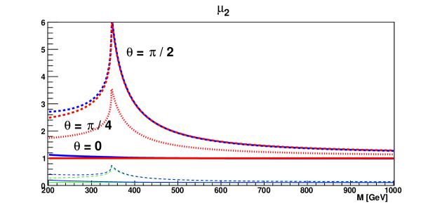
Figure 1: Cross section ratios $\mu_{2}$ for $gg$ production of $H_{2}$ for $\bar{\rho}^{q}$ defined by eq. (4.38). Here, for illustration we assume that phases of $\hat{\rho}^{q}$ are the same for up- and down-type quarks, so $\theta_{u}=\theta_{d}=\theta$. Red, heavy: general model with $|\hat{\rho}^{u}|=|\hat{\rho}^{d}|=1$ with (solid) $\theta=0$, (dotted) $\theta=\pi/4$ and (dashed) $\theta=\pi/2$. Blue (green) heavy solid: Type II (Type I) for $\tan\beta=1$ with $\alpha_{3}=0$ (so $H_{3}=A$). Dashed, same with $\alpha_{3}=\pi/2$ (so $H_{2}=A$). Thin (blue and green) Type I and Type II with $\tan\beta=3$. (The green curves, for Type I, are partly covered by the red and blue ones.) The spike at $M=2m_{t}$ originates from the function $\mbox{Re\thinspace}B$ of eq. (F.177) describing the pseudoscalar coupling.

To illustrate effects of generic Yukawa couplings in the production of $H_{2,3}$ we define

$$\mu_{\alpha}\equiv\frac{\sigma_{\alpha}}{\sigma_{\text{SM}}}=\frac{X_{\alpha}^{2}}{|A|^{2}_{\text{SM}}},$$ (5.4)

where $\alpha=2,3$, $\sigma_{\alpha}$ is the $pp\to H_{\alpha}$ $gg$ cross section in the 2HDM, $\sigma_{\text{SM}}$ is the corresponding SM cross section, and $X_{2}^{2}$ is given by eq.  (5.2). Here, $A_{\text{SM}}$ refers to the function (F.176), summed over $t$ and $b$-quark loops. In Fig. 1 we plot this quantity for $\alpha=2$.

It should be kept in mind that the normalization of this cross section depends critically on the assumed magnitudes $|\bar{\rho}|$, in particular on $|\bar{\rho}^{u}|$. The assumption of eq. (4.38) reproduces the predictions of the Type I and Type II models with $\tan\beta=1$, unless $\bar{\rho}$ has a non-zero phase $\theta$. In the latter case, if $\theta_{t}$ is non-zero, the production cross section would have a spike at the $t\bar{t}$ threshold.

6 “Heavy” Higgs boson decays in the approximate AL

It is important to realize that in the AL the $H_{2}$ and $H_{3}$ couplings are strongly correlated allowing for construction of observables that may efficiently test the alignment scenario.

There are four classes of interesting decay modes: final fermion-antifermion pairs, purely scalar decays, and final states involving a heavy gauge boson. We shall discuss them in the following subsections.

6.1 Fermionic modes

Table 1 summarizes Yukawa couplings in the AL for the generic model adopting the assumption of eq. (4.38) together with corresponding couplings for the Type I and Type II models (consistently also in the AL) used below as reference models to compare with 2HDM67 results. Note the 2HDM67 Yukawa couplings for the case of eq. (4.38) are parametrized by the quark masses and six additional independent numbers ($\mbox{Re\thinspace}\hat{\rho}^{l}$, $\mbox{Im\thinspace}\hat{\rho}^{l}$, $\mbox{Re\thinspace}\hat{\rho}^{d}$, $\mbox{Im\thinspace}\hat{\rho}^{d}$, $\mbox{Re\thinspace}\hat{\rho}^{u}$, $\mbox{Im\thinspace}\hat{\rho}^{u}$) while for the Type I or Type II the freedom is much more limited as the couplings can be specified by only two parameters ($\beta$, $\alpha_{3}$) with $\alpha_{3}=0,\pm\pi/2$.

Adopting eq. (4.38) one finds

$$\Gamma(H_{2}\to f_{3}\bar{f}_{3}) = \frac{3M_{2}}{8\pi}\frac{m_{f_{3}}^{2}}{v^{2}}\left((\mbox{Re\thinspace}\hat{\rho}^{f})^{2}\beta_{f_{3}2}^{2}+(\mbox{Im\thinspace}\hat{\rho}^{f})^{2}\right)\beta_{f_{3}2},$$ (6.1)

$$\Gamma(H_{3}\to f_{3}\bar{f}_{3}) = \frac{3M_{3}}{8\pi}\frac{m_{f_{3}}^{2}}{v^{2}}\left((\mbox{Im\thinspace}\hat{\rho}^{f})^{2}\beta_{f_{3}3}^{2}+(\mbox{Re\thinspace}\hat{\rho}^{f})^{2}\right)\beta_{f_{3}3}.$$ (6.2)

for $f_{3}=\tau,b,t$ and $\beta_{f\,\alpha}\equiv\sqrt{1-4m_{f}^{2}/M_{\alpha}^{2}}$. With the exception of the case of final state top quarks, we may approximate $\beta_{f\,\alpha}\sim 1$. Note that when $\beta_{f\,\alpha}\sim 1$ then the relations of eq. (4.33) imply that the squared matrix elements for $H_{2}\to f\bar{f}$ and $H_{3}\to f\bar{f}$ are nearly the same, so that the corresponding widths differ only by the overall scalar masses, therefore for $f_{3}\neq t$ one expects

$$\frac{\Gamma(H_{2}\to f_{3}\bar{f}_{3})}{\Gamma(H_{3}\to f_{3}\bar{f}_{3})}=\frac{M_{2}}{M_{3}}+{\cal{O}}\left(\frac{m_{f_{3}}^{2}}{M_{2,3}^{2}}\right).$$ (6.3)

	Type I	Type II	2HDM67
$a_{kk}^{2\,d}$	$-\frac{m_{d_{k}}}{v}c_{3}\frac{c_{\beta}}{s_{\beta}}$	$\phantom{-}\frac{m_{d_{k}}}{v}c_{3}\frac{s_{\beta}}{c_{\beta}}$	$-\delta_{k3}\frac{m_{b}}{v}\mbox{Re\thinspace}\hat{\rho}^{d}$
$a_{kk}^{3\,d}$	$\phantom{-}\frac{m_{d_{k}}}{v}s_{3}\frac{c_{\beta}}{s_{\beta}}$	$-\frac{m_{d_{k}}}{v}s_{3}\frac{s_{\beta}}{c_{\beta}}$	$-\delta_{k3}\frac{m_{b}}{v}\mbox{Im\thinspace}\hat{\rho}^{d}$
$b_{kk}^{2\,d}$	$-\frac{m_{d_{k}}}{v}s_{3}\frac{c_{\beta}}{s_{\beta}}$	$\phantom{-}\frac{m_{d_{k}}}{v}s_{3}\frac{s_{\beta}}{c_{\beta}}$	$\phantom{-}\delta_{k3}\frac{m_{b}}{v}\mbox{Im\thinspace}\hat{\rho}^{d}$
$b_{kk}^{3\,d}$	$-\frac{m_{d_{k}}}{v}c_{3}\frac{c_{\beta}}{s_{\beta}}$	$\phantom{-}\frac{m_{d_{k}}}{v}c_{3}\frac{s_{\beta}}{c_{\beta}}$	$-\delta_{k3}\frac{m_{b}}{v}\mbox{Re\thinspace}\hat{\rho}^{d}$
$a_{kk}^{2\,u}$	$-\frac{m_{u_{k}}}{v}c_{3}\frac{c_{\beta}}{s_{\beta}}$	$-\frac{m_{u_{k}}}{v}c_{3}\frac{c_{\beta}}{s_{\beta}}$	$-\delta_{k3}\frac{m_{t}}{v}\mbox{Re\thinspace}\hat{\rho}^{u}$
$a_{kk}^{3\,u}$	$\phantom{-}\frac{m_{u_{k}}}{v}s_{3}\frac{c_{\beta}}{s_{\beta}}$	$\phantom{-}\frac{m_{u_{k}}}{v}s_{3}\frac{c_{\beta}}{s_{\beta}}$	$-\delta_{k3}\frac{m_{t}}{v}\mbox{Im\thinspace}\hat{\rho}^{u}$
$b_{kk}^{2\,u}$	$\phantom{-}\frac{m_{u_{k}}}{v}s_{3}\frac{c_{\beta}}{s_{\beta}}$	$\phantom{-}\frac{m_{u_{k}}}{v}s_{3}\frac{c_{\beta}}{s_{\beta}}$	$-\delta_{k3}\frac{m_{t}}{v}\mbox{Im\thinspace}\hat{\rho}^{u}$
$b_{kk}^{3\,u}$	$\phantom{-}\frac{m_{u_{k}}}{v}c_{3}\frac{c_{\beta}}{s_{\beta}}$	$\phantom{-}\frac{m_{u_{k}}}{v}c_{3}\frac{c_{\beta}}{s_{\beta}}$	$\phantom{-}\delta_{k3}\frac{m_{t}}{v}\mbox{Re\thinspace}\hat{\rho}^{u}$

Table 1: Couplings $a_{kk}^{\alpha\,q}$ and $b_{kk}^{\alpha\,q}$ for the Type I, Type II models and for the generic 2HDM in the AL. For 2HDM5 one should consider the two cases: $\alpha_{3}=0$ and $\alpha_{3}=\pm\pi/2$. For the 2HDM67 the assumption of eq. (4.38) was adopted.

It is useful to define the reduced width for fermionic two-body Higgs boson decays,

$$\bar{\Gamma}(H_{\alpha}\to f\bar{f})\equiv\frac{8\pi}{3M_{\alpha}}\Gamma(H_{\alpha}\to f\bar{f})\left(\frac{v}{m_{f}}\right)^{2}\beta_{f\,\alpha}^{-1},$$ (6.4)

with $\alpha=2,3$. In Table 2 we collect predictions for $\tau^{+}\tau^{-}$, $b\bar{b}$, $c\bar{c}$, and $t\bar{t}$ reduced decay widths $\bar{\Gamma}$ in the Type I and Type II models and compare to the 2HDM67.

$\bar{\Gamma}(H_{\alpha}\to f\bar{f})$	Type I	Type II	2HDM67
$\bar{\Gamma}(H_{2,3}\to\tau^{+}\tau^{-})$	$\left(\frac{c_{\beta}}{s_{\beta}}\right)^{2}$	$\left(\frac{s_{\beta}}{c_{\beta}}\right)^{2}$	$|\hat{\rho}^{l}|^{2}$
$\bar{\Gamma}(H_{2,3}\to b\bar{b})$	$\left(\frac{c_{\beta}}{s_{\beta}}\right)^{2}$	$\left(\frac{s_{\beta}}{c_{\beta}}\right)^{2}$	$|\hat{\rho}^{d}|^{2}$
$\bar{\Gamma}(H_{2}\to c\bar{c})$	$\left(\frac{c_{\beta}}{s_{\beta}}\right)^{2}$	$\left(\frac{c_{\beta}}{s_{\beta}}\right)^{2}$	$0$
$\bar{\Gamma}(H_{2}\to t\bar{t})$	$\left(\frac{c_{\beta}}{s_{\beta}}\right)^{2}(c_{3}^{2}\beta_{t\,2}^{2}+s_{3}^{2})$	$\left(\frac{c_{\beta}}{s_{\beta}}\right)^{2}(c_{3}^{2}\beta_{t\,2}^{2}+s_{3}^{2})$	$(\mbox{Re\thinspace}\hat{\rho}^{u})^{2}\beta_{t\,2}^{2}+(\mbox{Im\thinspace}\hat{\rho}^{u})^{2}$
$\bar{\Gamma}(H_{3}\to t\bar{t})$	$\left(\frac{c_{\beta}}{s_{\beta}}\right)^{2}(s_{3}^{2}\beta_{t\,2}^{2}+c_{3}^{2})$	$\left(\frac{c_{\beta}}{s_{\beta}}\right)^{2}(s_{3}^{2}\beta_{t\,3}^{2}+c_{3}^{2})$	$(\mbox{Im\thinspace}\hat{\rho}^{u})^{2}\beta_{t\,3}^{2}+(\mbox{Re\thinspace}\hat{\rho}^{u})^{2}$

Table 2: Rescaled decay widths $\bar{\Gamma}$ for $\tau^{+}\tau^{-}$, $b\bar{b}$, $c\bar{c}$, and $t\bar{t}$ final states in the AL. For $\tau$, $b$, and $c$, $\beta_{f\,\alpha}$ was approximated by 1. For the 2HDM67 the assumption of eq. (4.38) was adopted.

The correlations between $H_{2}$ and $H_{3}$ decay widths are clearly seen from Table 2. Note first of all that for the light fermions the reduced widths are equal for $H_{2}$ and $H_{3}$, $\bar{\Gamma}(H_{2}\to f\bar{f})=\bar{\Gamma}(H_{3}\to f\bar{f})$, this is a consequence of the alignment and could be explored to test this scenario. Note however that since it holds also in the Type I and Type II models, it can not be used to disentangle various versions of 2HDM5. The extra freedom provided within the 2HDM67 is also seen from the table, e.g. in the Type I and Type II models $\bar{\Gamma}(H_{2,3}\to\tau^{+}\tau^{-})\simeq\bar{\Gamma}(H_{2,3}\to b\bar{b})$, while in 2HDM67 the reduced widths might be different. Note that for the Type I and Type II models leptonic-, down- and up-type widths are correlated while within 2HDM67 they are independent. Of course, the most straightforward way to disentangle Type I, II and 2HDM67 in the AL is to look for FCNC in $H_{2,3}$ decays, since they are not present in the former models while they may appear in the 2HDM67 at the tree level. Of course, the discovery of FCNC by itself would not test the alignment scenario as one would need to verify the correlations between the $H_{2}$ and $H_{3}$ couplings (and therefore their widths) encoded in eqs. (4.34)–(4.35).

For $t\bar{t}$ final states the AL might be tested just by measuring $\bar{\Gamma}_{t\,2,3}$, if a solution with respect to $\mbox{Im\thinspace}\hat{\rho}^{u}$ and $\mbox{Re\thinspace}\hat{\rho}^{u}$ exists then the measurement agrees with the AL. Note that the same measurement could also be interpreted within Type I or Type II. Then, if eq. (4.8) is adopted in Table 2 one obtains for Type I and II the following, $\beta$-dependent relation

$$\frac{\bar{\Gamma}(H_{2}\to\bar{t}t)}{\bar{\Gamma}(H_{3}\to\bar{t}t)}=\left\{\begin{tabular}[]{ll}$\beta_{t\,2}^{2}$&$\alpha_{3}=0$\\ $\beta_{t\,3}^{-2}$&$\alpha_{3}=\pm\pi/2$\end{tabular}\right.$$ (6.5)

If $\Gamma_{2,3}$ and masses were measured, then eq. (6.5) could be verified in order to test the alignment scenario for the Type I and II models.

For completeness and future reference we exhibit below the most general Yukawa couplings, expanded up to linear order in $e_{2,3}/v$:

$$\bar{l}_{k}l_{l}H_{1}: -\frac{m_{k}}{v}\delta_{lk}+\frac{1}{2\sqrt{2}v}\left[\left(\bar{\rho}^{l}_{lk}\right)^{*}(1+\gamma_{5})(e_{2}+ie_{3})+\bar{\rho}^{l}_{kl}(1-\gamma_{5})(e_{2}-ie_{3})\right],$$ (6.6)

$$\bar{d}_{k}d_{l}H_{1}: -\frac{m_{d_{l}}}{v}\delta_{lk}+\frac{1}{2\sqrt{2}v}\left[\left(\bar{\rho}^{d}_{lk}\right)^{*}(1+\gamma_{5})(e_{2}+ie_{3})+\bar{\rho}^{d}_{kl}(1-\gamma_{5})(e_{2}-ie_{3})\right],$$ (6.7)

$$\bar{u}_{k}u_{l}H_{1}: -\frac{m_{u_{k}}}{v}\delta_{lk}+\frac{1}{2\sqrt{2}v}\left[\left(\bar{\rho}^{u}_{lk}\right)^{*}(1-\gamma_{5})(e_{2}+ie_{3})+\bar{\rho}^{u}_{kl}(1+\gamma_{5})(e_{2}-ie_{3})\right].$$ (6.8)

Below, $\alpha=2$ or $3$:

$$\bar{l}_{k}l_{l}H_{\alpha}: -\frac{m_{k}}{v^{2}}e_{\alpha}\delta_{lk}+\frac{i^{\alpha}}{2\sqrt{2}}\left[\left(\bar{\rho}^{l}_{lk}\right)^{*}(1+\gamma_{5})+(-1)^{\alpha}\bar{\rho}^{l}_{kl}(1-\gamma_{5})\right],$$ (6.9)

$$\bar{d}_{k}d_{l}H_{\alpha}: -\frac{m_{d_{l}}}{v^{2}}e_{\alpha}\delta_{lk}+\frac{i^{\alpha}}{2\sqrt{2}}\left[\left(\bar{\rho}^{d}_{lk}\right)^{*}(1+\gamma_{5})+(-1)^{\alpha}\bar{\rho}^{d}_{kl}(1-\gamma_{5})\right],$$ (6.10)

$$\bar{u}_{k}u_{l}H_{\alpha}: -\frac{m_{u_{k}}}{v^{2}}e_{\alpha}\delta_{lk}+\frac{i^{\alpha}}{2\sqrt{2}}\left[\left(\bar{\rho}^{u}_{lk}\right)^{*}(1-\gamma_{5})+(-1)^{\alpha}\bar{\rho}^{u}_{kl}(1+\gamma_{5})\right].$$ (6.11)

These results show that in the case of a broken ${\mathbbm{Z}}_{2}$ symmetry, both flavor-nondiagonal Yukawa couplings of $H_{2,3}$ and new CPV Yukawa couplings are present even in the AL. Of course, there exist experimental constraints on FCNCs, e.g. measured upper limits for $BR(B_{s}\to\mu^{+}\mu^{-})$ or $B_{s,d}^{0}$–$\overline{B}^{\lower 6.0pt\hbox{$\scriptstyle 0$}}_{s,d}$ mixing that constrain the flavor-nondiagonal Yukawa couplings of the neutral Higgs bosons. For example, the experimental measurements of the latter roughly imply that

$$\frac{m_{b}m_{k}}{M_{\alpha}^{2}}\times\left\{\left|\bar{\rho}^{d}_{bk}\right|^{2},\left|\bar{\rho}^{d}_{kb}\right|^{2},\left|\bar{\rho}^{d}_{bk}\bar{\rho}^{d\,\star}_{kb}\right|\right\}\ll 1\,,$$ (6.12)

for $k=d,s$ and $\alpha=2,3$. The above constraints would be naturally satisfied in the AL with decoupling for $M_{2,3}\mathrel{\raise 1.29167pt\hbox{$>$\kern-7.5pt\lower 4.30554pt\hbox{$\sim$}}}10\;\hbox{TeV}$. In contrast, in the AL without decoupling with $M_{2,3}\sim{\cal O}(100)\;\hbox{GeV}$, the $\bar{\rho}^{d}_{bk}$ must be sufficiently suppressed. On the other hand, the presence of some Higgs-mediated FCNCs could be seen as an advantage of the model given that not all FCNC couplings are significantly constrained by experiment (as in the case of FCNCs involving the top quark, which could show up in future experimental studies).

6.2 Bosonic decays

As we have already seen, fermionic decays of Higgs bosons in the generic model suffer from the presence of many unknown parameters encoded into the $\rho$ matrices. Therefore it is reasonable to consider only the exact AL while investigating fermionic decays. However for bosonic decays we are going to expand the potential around the alignment up to linear terms in $e_{2}/v$ and $e_{3}/v$. For vector-scalar decay modes we need to expand also the $f_{i}$ coefficients up to linear order in $e_{2}/v$ and $e_{3}/v$

$$f_{1} = -\tilde{f}\left(\frac{e_{2}}{v}-i\frac{e_{3}}{v}\right),$$ (6.13)

$$f_{2} = \tilde{f},\;\;\;\;\;f_{3}=-i\tilde{f}$$ (6.14)

for $\tilde{f}=v(c_{3}-is_{3})$.

operator	exact AL	${\cal{O}}(e_{2}/v)$	${\cal{O}}(e_{3}/v)$
$H_{1}H_{1}H_{1}$	$M_{1}^{2}/(2v)$	0	0
$H_{2}H_{2}H_{2}$	${\textstyle\frac{1}{2}}q_{2}$	$(M_{2}^{2}-M_{H^{\pm}}^{2})/v$	$0$
$H_{3}H_{3}H_{3}$	${\textstyle\frac{1}{2}}q_{3}$	$0$	$(M_{3}^{2}-M_{H^{\pm}}^{2})/v$
$H_{1}H_{1}H_{2}$	0	$(4M_{H^{\pm}}^{2}-M_{2}^{2}-2vq_{1})/(2v)$	$0$
$H_{1}H_{1}H_{3}$	0	$0$	$(4M_{H^{\pm}}^{2}-M_{3}^{2}-2vq_{1})/(2v)$
$H_{2}H_{2}H_{1}$	$(2M_{2}^{2}-2M_{H^{\pm}}^{2}+vq_{1})/(2v)$	$-q_{2}$	$0$
$H_{3}H_{3}H_{1}$	$(2M_{3}^{2}-2M_{H^{\pm}}^{2}+vq_{1})/(2v)$	$0$	$-q_{3}$
$H_{2}H_{2}H_{3}$	${\textstyle\frac{1}{2}}q_{3}$	$0$	$(M_{2}^{2}-M_{H^{\pm}}^{2})/v$
$H_{3}H_{3}H_{2}$	${\textstyle\frac{1}{2}}q_{2}$	$(M_{3}^{2}-M_{H^{\pm}}^{2})/v$	$0$
$H_{1}H_{2}H_{3}$	$0$	$-q_{3}$	$-q_{2}$
$H_{i}H^{-}H^{+}$	$q_{i}$	$0$	$0$

Table 3: Coefficients of cubic (non-Goldstone) scalar operators expanded around the alignment limit (AL) without decoupling up to ${\cal{O}}(e_{2,3}/v)$. The second, third and fourth columns show the exact alignment result and coefficients of $e_{2}/v$ and $e_{3}/v$, respectively. If the alignment limit is realized via decoupling, then certain results of this table are modified as shown in Table 4.

operator	exact AL	${\cal{O}}(e_{2}/v)$	${\cal{O}}(e_{3}/v)$
$H_{1}H_{1}H_{1}$	$M_{1}^{2}/(2v)$	$-e_{2}M_{H^{\pm}}^{2}/v^{2}$	$-e_{3}M_{H^{\pm}}^{2}/v^{2}$
$H_{1}H_{1}H_{2}$	$3e_{2}M^{2}_{2}/(2v^{2})$	$(2M_{H^{\pm}}^{2}-2M_{2}^{2}-vq_{1})/v$	$0$
$H_{1}H_{1}H_{3}$	$3e_{3}M^{2}_{3}/(2v^{2})$	$0$	$(2M_{H^{\pm}}^{2}-2M_{3}^{2}-vq_{1})/v$
$H_{2}H_{2}H_{1}$	$(2M_{2}^{2}-2M_{H^{\pm}}^{2}+vq_{1})/(2v)$	$-q_{2}+2e_{2}M_{2}^{2}/v^{2}$	$0$
$H_{3}H_{3}H_{1}$	$(2M_{3}^{2}-2M_{H^{\pm}}^{2}+vq_{1})/(2v)$	$0$	$-q_{3}+2e_{3}M_{3}^{2}/v^{2}$
$H_{1}H_{2}H_{3}$	$0$	$-q_{3}+2e_{3}M_{3}^{2}/v^{2}$	$-q_{2}+2e_{2}M_{2}^{2}/v^{2}$

Table 4: Coefficients of cubic scalar operators expanded around the alignment limit (AL), where the alignment is realized via decoupling, up to ${\cal{O}}(e_{2,3}/v)$. See caption to Table 3. Note that $e_{2}M^{2}$ and $e_{3}M^{2}$ (for $M=M_{2}$, $M_{3}$ or $M_{H^{\pm}}$) approach a finite nonzero value in the limit of exact decoupling (i.e., as $M\to\infty$). Further explanations are provided in the text.

Since we are going to focus on two-body Higgs boson decays, in Tables 3–5 we collect coefficients of cubic bosonic operators expanded around the AL up to linear terms in $e_{2}/v$ and $e_{3}/v$. One subtlety in obtaining the results of Table 3 is the distinction between achieving the alignment limit via decoupling or in the absence of decoupling. We illustrate this point by examining the $H_{1}H_{1}H_{2}$ coupling. Eq. (B.10) yields the following coefficient of the $H_{1}H_{1}H_{2}$ operator in the scalar potential,

$$H_{1}H_{1}H_{2}:\quad-\frac{e_{1}e_{2}}{v^{2}}q_{1}+\frac{v^{2}-e_{1}^{2}}{2v^{2}}q_{2}+\frac{(3e_{1}^{2}-v^{2})e_{2}}{v^{4}}M^{2}_{H^{\pm}}+\frac{(v^{2}-e_{1}^{2})e_{2}}{v^{4}}M_{1}^{2}-\frac{e_{1}^{2}e_{2}}{2v^{4}}M_{2}^{2}\,.$$ (6.15)

In the approximate alignment limit without decoupling, all scalar squared masses are of $\mathcal{O}(v^{2})$. In light of Table 8, the coefficient of the $H_{1}H_{1}H_{2}$ operator is

$$v\left[\frac{e_{2}(4M_{H^{\pm}}^{2}-M_{2}^{2}-2vq_{1})}{2v^{3}}+\mathcal{O}(e_{2}^{2}/v^{2},e_{3}^{2}/v^{2})\right]\,,$$ (6.16)

where we have explicitly exhibited the terms of $\mathcal{O}(e_{2}/v)$ inside the bracketed expression above [note that there are no terms of $\mathcal{O}(e_{3}/v)$]. In the exact alignment limit (where we set $e_{2}=e_{3}=0$), the coefficient of the $H_{1}H_{1}H_{2}$ operator vanishes. In contrast, in the decoupling regime, $M^{2}_{2}$, $M_{H^{\pm}}^{2}\gg v^{2}$, and the expansion in the small parameters is organized differently. In particular, using the results of Appendix D.3, one can derive eq. (D.93), which yields,

$$e_{2}M^{2}\simeq v^{3}\mbox{Re\thinspace}(Z_{6}e^{-i\theta_{23}})\,,\qquad\quad e_{3}M^{2}\simeq-v^{3}\mbox{Im\thinspace}(Z_{6}e^{-i\theta_{23}})\,,\quad\text{for $M=M_{2},M_{3},M_{H^{\pm}}$}\,,$$ (6.17)

where $Z_{6}$ is an $\mathcal{O}(1)$ parameter that appears in the scalar potential expressed in terms of the Higgs basis fields [cf. eq. (D.49)], and $\theta_{23}$ is a mixing angle introduced in eq. (D.55). Hence, in the exact alignment limit in the decoupling regime, eq. (6.16) yields $3e_{2}M^{2}_{2}/(2v^{2})$, which is finite and nonzero as $M_{2}\to\infty$ in light of eq. (6.17). The first order correction to this result is

$$\frac{e_{2}\bigl{[}2(M_{H^{\pm}}^{2}-M_{2}^{2})-vq_{1}\bigr{]}}{v^{2}}\,,$$ (6.18)

where the difference in the squared masses above is given by eq. (D.92). Similar considerations apply to the $H_{1}H_{1}H_{3}$ operator in Table 3.

Similarly, in the $\mathcal{O}(e_{2}/v)$ and $\mathcal{O}(e_{3}/v)$ entries for the $H_{1}H_{1}H_{1}$, $H_{2}H_{2}H_{1}$, $H_{3}H_{3}H_{1}$ and $H_{1}H_{2}H_{3}$ operators, the results presented in Table 3 do not include terms that are of $\mathcal{O}(e^{2}_{2}M^{2}/v^{3})$ and $\mathcal{O}(e^{3}_{2}M^{2}/v^{3})$, where $M=M_{2},M_{3}$ or $M_{H^{\pm}}$. Such terms are quadratically suppressed in the approximate alignment limit without decoupling. But in the decoupling regime, eq. (6.17) implies that such terms would compete with those terms listed in Table 3. Thus, in Table 4, we provide the exact alignment results and the corresponding first order corrections for those cubic Higgs operators that differ from the results displayed in Table 3.

operator	exact AL	${\cal{O}}(e_{2}/v)$	${\cal{O}}(e_{3}/v)$
$H_{1}H^{+}W^{-}_{\mu}$	$0$	$-\frac{ig}{2v}\tilde{f}(p_{1}-p^{+})_{\mu}$	$-\frac{g}{2v}\tilde{f}(p_{1}-p^{+})_{\mu}$
$H_{1}H^{-}W^{+}_{\mu}$	$0$	$+\frac{ig}{2v}\tilde{f}^{\ast}(p_{1}-p^{-})_{\mu}$	$-\frac{g}{2v}\tilde{f}^{\ast}(p_{1}-p^{-})_{\mu}$
$H_{2}H^{+}W^{-}_{\mu}$	$+\frac{ig}{2v}\tilde{f}(p_{2}-p^{+})_{\mu}$	$0$	$0$
$H_{2}H^{-}W^{+}_{\mu}$	$-\frac{ig}{2v}\tilde{f}^{\ast}(p_{2}-p^{-})_{\mu}$	$0$	$0$
$H_{3}H^{+}W^{-}_{\mu}$	$+\frac{g}{2v}\tilde{f}(p_{3}-p^{+})_{\mu}$	$0$	$0$
$H_{3}H^{-}W^{+}_{\mu}$	$+\frac{g}{2v}\tilde{f}^{\ast}(p_{3}-p^{-})_{\mu}$	$0$	$0$
$H_{1}H_{2}Z_{\mu}$	$0$	$0$	$\frac{g}{2\cos\theta_{W}}(p_{1}-p_{2})_{\mu}$
$H_{2}H_{3}Z_{\mu}$	$\frac{g}{2\cos\theta_{W}}(p_{2}-p_{3})_{\mu}$	$0$	$0$
$H_{3}H_{1}Z_{\mu}$	$0$	$\frac{g}{2\cos\theta_{W}}(p_{3}-p_{1})_{\mu}$	$0$
$H_{1}Z_{\mu}Z_{\nu}$	$\frac{ig^{2}v}{2\cos^{2}\theta_{W}}g_{\mu\nu}$	$0$	$0$
$H_{2}Z_{\mu}Z_{\nu}$	$0$	$\frac{ig^{2}v}{2\cos^{2}\theta_{W}}g_{\mu\nu}$	$0$
$H_{3}Z_{\mu}Z_{\nu}$	$0$	$0$	$\frac{ig^{2}v}{2\cos^{2}\theta_{W}}g_{\mu\nu}$
$H_{1}W^{+}_{\mu}W^{-}_{\nu}$	$\frac{ig^{2}v}{2}g_{\mu\nu}$	$0$	$0$
$H_{2}W^{+}_{\mu}W^{-}_{\nu}$	$0$	$\frac{ig^{2}v}{2}g_{\mu\nu}$	$0$
$H_{3}W^{+}_{\mu}W^{-}_{\nu}$	$0$	$0$	$\frac{ig^{2}v}{2}g_{\mu\nu}$

Table 5: Coefficients of $H_{i}H^{+}W^{-}_{\mu}$, $H_{i}H^{-}W^{+}_{\mu}$, $H_{i}H_{j}Z_{\mu}$, $H_{i}Z_{\mu}Z_{\nu}$ and $H_{i}W^{+}_{\mu}W^{-}_{\nu}$ operators expanded around the AL up to ${\cal{O}}(e_{2,3}/v)$. The second, third and fourth columns show the alignment result and coefficients of $e_{2}/v$ and $e_{3}/v$, respectively.

$\Gamma$	decay process
${\cal{O}}(1)$	$H^{\pm}\to H_{2,3}W^{\pm}$, $H_{2,3}\to H^{+}H^{-}$, $H_{2,3}\to H_{1}H_{1}$ (DL), $H_{3}\to H_{2}H_{2}$, $H_{3}\to H_{2}Z$
${\cal{O}}\big{[}\left(\frac{e_{2}}{v}\right)^{2}\big{]}$	$H_{3}\to H_{1}Z$, $H_{2}\to ZZ$, $H_{2}\to W^{+}W^{-}$, $H_{2}\to H_{1}H_{1}$
${\cal{O}}\big{[}\left(\frac{e_{3}}{v}\right)^{2}\big{]}$	$H_{2}\to H_{1}Z$, $H_{3}\to ZZ$, $H_{3}\to W^{+}W^{-}$, $H_{3}\to H_{1}H_{1}$
${\cal{O}}\big{[}\left(\frac{e_{2}}{v}\right)^{2},\left(\frac{e_{3}}{v}\right)^{2},\frac{e_{2}e_{3}}{v^{2}}\big{]}$	$H_{3}\to H_{2}H_{1}$

Table 6: Possible two-body decays of heavy Higgs bosons classified according to the strength of the corresponding decay width. The first row shows leading decays that exist in the AL, the second and third rows show decays the width of which is suppressed by $(e_{2}/v)^{2}$ and $(e_{3}/v)^{2}$, respectively, while the fourth one contains decays with the width suppressed by $\max[(e_{2}/v)^{2},(e_{3}/v)^{2},(e_{2}e_{3}/v^{2})]$. As noted in the text [cf. Tables 3 and 4], if approximate alignment is achieved in the decoupling limit (DL), then the coefficient of the $H_{1}H_{1}H_{k}$ operator (for $k=2,3$) in the exact alignment limit is nonzero and hence unsuppressed.

In Table 6 we combine predictions for bosonic Higgs boson two-body decays. Note that ratios of decay widths for processes contained in the second and third rows of Table 6 are functions of masses of the involved particles only, as the couplings proportional to $e_{2}$ and $e_{3}$ cancel out. Therefore, even though the widths are expected to be small, predictions for their ratios are quite unambiguous, depending on masses of the involved particles only.

6.2.1 Scalar-scalar modes

Among the leading, unsuppressed decays contained in the first row of Table 6 only two purely scalar decays $H_{3}\to H^{+}H^{-}$, $H_{3}\to H_{2}H_{2}$ are subject of some extra uncertainties as they are both $\propto q_{3}$, however their ratio

$$\frac{\text{BR}(H_{3}\to H^{+}H^{-})}{\text{BR}(H_{3}\to H_{2}H_{2})}=\sqrt{\frac{M_{3}^{2}-4M_{H^{\pm}}^{2}}{M_{3}^{2}-4M_{2}^{2}}}\left[1-\frac{4(M_{2}^{2}-M_{H^{\pm}}^{2})}{q_{3}v}\frac{e_{3}}{v}+\mathcal{O}(e_{2}^{2}/v^{2},e_{2}e_{3}/v^{2},e_{3}^{2}/v^{2})\right],$$ (6.19)

depends only on the masses of the particles involved in the decays and therefore might be useful for testing this scenario. Note that in the 2HDM5 models $H_{3}\to H^{+}H^{-}$ and $H_{3}\to H_{2}H_{2}$ decays exist only if $\alpha_{3}=\pm\pi/2$ ($A=H_{2}$ and $H=H_{3}$). In the case of $\alpha_{3}=0$ ($A=H_{3}$ and $H=H_{2}$) the corresponding widths vanish at the tree level.

Furthermore, as seen from Table 6, we find that to the leading order

$$\text{BR}(H_{3}\to H_{1}H_{2})=\mathcal{O}(e_{2}^{2}/v^{2},e_{2}e_{3}/v^{2},e_{3}^{2}/v^{2}).$$ (6.20)

In contrast, the decay rate for $H_{2,3}\to H_{1}H_{1}$ may or may not be suppressed depending on whether approximate alignment is achieved with or without decoupling. Indeed as previously noted, the leading contribution to the $H_{k}H_{1}H_{1}$ coupling (for $k=2,3$) is proportional to $e_{k}M_{k}^{2}/v^{2}\sim\mathcal{O}(v)$ in the limit of large $M_{k}\gg v$ and hence unsuppressed.

6.2.2 Scalar-vector modes

In this subsection, we consider Higgs decay modes into two-body $VV$ and $VH$ final states (for $V=W^{\pm}$ or $Z$ and $H=H_{1,2,3},H^{\pm}$). In the AL, $H_{1}$ couples to the vector bosons as in the SM, whereas the decay rates for the modes $H_{2,3}\to W^{+}W^{-}$, $H_{2,3}\to ZZ$ and $H_{2,3}\to H_{1}Z$ all vanish, since their couplings are proportional to $e_{2,3}=0$. Hence, it follows that

$$\frac{\Gamma(H_{1}\to W^{+}W^{-},ZZ)}{\Gamma(H_{\text{SM}}\to W^{+}W^{-},ZZ)} = 1+\mathcal{O}(e_{2}^{2}/v^{2},e_{2}e_{3}/v^{2},e_{3}^{2}/v^{2}),$$ (6.21)

$$\text{BR}(H_{2,3}\to W^{+}W^{-},ZZ,H_{1}Z) = \mathcal{O}(e_{2}^{2}/v^{2},e_{2}e_{3}/v^{2},e_{3}^{2}/v^{2}).$$ (6.22)

The couplings $H_{2}H^{+}W^{-}$ and $H_{3}H^{+}W^{-}$ differ by a phase factor only, so that (if kinematically open)

$$\frac{\text{BR}(H^{\pm}\to H_{2}W^{\pm})}{\text{BR}(H^{\pm}\to H_{3}W^{\pm})}=\frac{\left[\lambda(M_{H^{\pm}},M_{2},M_{W})\right]^{3/2}}{\left[\lambda(M_{H^{\pm}},M_{3},M_{W})\right]^{3/2}}+\mathcal{O}(e_{2}^{2}/v^{2},e_{2}e_{3}/v^{2},e_{3}^{2}/v^{2}).$$ (6.23)

Similarly, the couplings $H_{3}H^{+}W^{-}$ and $H_{3}H_{2}Z$ differ by a phase and a trivial factor only, so

$$\frac{\text{BR}(H_{3}\to H_{2}Z)}{\text{BR}(H_{3}\to H^{+}W^{-})}=\frac{1}{c_{W}^{2}}\frac{\left[\lambda(M_{3},M_{2},M_{Z})\right]^{3/2}}{\left[\lambda(M_{3},M_{H^{\pm}},M_{W})\right]^{3/2}}+\mathcal{O}(e_{2}^{2}/v^{2},e_{2}e_{3}/v^{2},e_{3}^{2}/v^{2}).$$ (6.24)

The observables defined above do not differentiate between the 2HDM5 and 2HDM67 models.

Since in the AL $f_{1}=0$ therefore

$$\text{BR}(H^{\pm}\to W^{\pm}H_{1})=\mathcal{O}(e_{2}^{2}/v^{2},e_{2}e_{3}/v^{2},e_{3}^{2}/v^{2}).$$ (6.25)

This holds both for the 2HDM5 and 2HDM67 models.

Note that for the $VV$ and $VH$ final states discussed in this subsection, the leading corrections to the AL results appear at the quadratic level, i.e., there are no corrections linear in $e_{2,3}$. Therefore the above predictions in the AL are rather robust.

7 Summary

Given that the observed couplings of the Higgs boson are SM-like and the $\rho$ parameter is measured to be near $1$, models of extended Higgs sectors are significantly constrained. The generic two Higgs doublet model (2HDM) unconstrained by a ${\mathbbm{Z}}_{2}$ symmetry provides a simple extension of the SM with new sources of CP violation in the scalar sector. In this paper, the phenomenology of the approximate alignment limit of the 2HDM in which the $125\;\hbox{GeV}$ Higgs boson couplings are close to those of the SM has been discussed in detail. The alignment limit can be achieved with or without the decoupling of the heavier Higgs states of the scalar sector. Indeed, regions of the 2HDM parameter space exist in which at least some of the heavier scalar states have masses not significantly above the observed Higgs boson mass of $125\;\hbox{GeV}$, without being in conflict with the SM-like couplings of the discovered Higgs boson.

We have shown that all possible bosonic couplings of the 2HDM scalars can be expressed in terms of a minimal set of seven physical Higgs couplings and four scalar masses, which then yield numerous correlations among processes involving the interactions of the scalars. Some of these correlations are quite striking in the alignment limit; for example, $\text{BR}(H_{2,3}\to W^{+}W^{-},ZZ,ZH_{1})=0$ and $\text{BR}(H^{\pm}\to W^{\pm}H_{1})=0$. In addition, correlations between $H_{2}$ and $H_{3}$ couplings in the alignment limit imply that the ratios of branching ratios, $\text{BR}(H^{\pm}\to H_{2}W^{\pm})/\text{BR}(H^{\pm}\to H_{3}W^{\pm})$, $\text{BR}(H_{3}\to H_{2}Z)/\text{BR}(H_{3}\to H^{+}W^{-})$ for bosonic decays and $\Gamma(H_{2}\to f\bar{f})/\Gamma(H_{3}\to f\bar{f})$ for fermionic ones, are functions of masses only. Leading corrections ($\propto e_{2,3}$) to the alignment limit results for bosonic decays of $H_{2,3}$ have been also calculated. In particular, for the scalar-vector final states, the corrections to exact alignment are quadratic in small quantities, i.e. they are proportional to $e_{2}^{2},e_{2}e_{3}$ or $e_{3}^{2}$. Consequently, the alignment limit results for branching ratios into scalar-vector final states are quite robust.

In processes that involve the cubic or quartic scalar couplings, the implications of the alignment limit may depend on whether alignment is achieved via the decoupling of heavy scalar states. For example, we have shown that in the exact alignment limit without decoupling, BR($H_{2,3}\to H_{1}H_{1})=0$. In contrast, in the decoupling regime, this branching ratio is finite and non-zero.

For the Yukawa couplings, in addition to presenting the most general results, various special cases were considered, e.g. diagonal $\rho$ matrices, type I or II models, etc. Leading corrections to the exact alignment limit values have been also shown and expressed in terms of the (small, i.e. $\propto e_{2,3}$) couplings of the heavier scalars to the gauge bosons. It should be stressed that broken ${\mathbbm{Z}}_{2}$ implies not only new sources of CP-violation in the potential, but also extra CP-violating Yukawa couplings. Phenomenologically the latter might be even more relevant in future collider studies.

The absence of a ${\mathbbm{Z}}_{2}$ symmetry, even in the alignment limit, results in the presence of flavor-nondiagonal Yukawa couplings of the heavier neutral Higgs bosons. For some of them there exist severe experimental upper limits which would be satisfied in the alignment limit for sufficiently heavy non-SM-like Higgs boson masses (i.e., in the alignment limit with decoupling). In contrast, the alignment limit without decoupling with $M_{2,3}\sim{\cal O}(100)\;\hbox{GeV}$ requires a significant fine-tuning of the flavor-nondiagonal couplings to be consistent with experimental constraints. In this context, we note that current experimental constraints on flavor-nondiagonal neutral Higgs coupling to top quarks are quite weak. If evidence of such couplings emerge in future experiments, such phenomena could be easily accommodated in the generic 2HDM.

Appendix A Couplings involving gauge fields

By putting

$$D^{\mu} = \partial^{\mu}+\frac{ig}{2}\sigma_{i}W_{i}^{\mu}+i\frac{g^{\prime}}{2}B^{\mu},$$ (A.1)

with $W_{1}^{\mu}=\frac{1}{\sqrt{2}}(W^{+\mu}+W^{-\mu})$, $W_{2}^{\mu}=\frac{i}{\sqrt{2}}(W^{+\mu}-W^{-\mu})$, $W_{3}^{\mu}=\cos{\theta}_{\text{W}}Z^{\mu}+\sin{\theta}_{\text{W}}A^{\mu}$ and $B^{\mu}=-\sin{\theta}_{\text{W}}Z^{\mu}+\cos{\theta}_{\text{W}}A^{\mu}$, the kinetic part of the Lagrangian can be written

$${\cal L}_{k}=(D_{\mu}\Phi_{1})^{\dagger}(D^{\mu}\Phi_{1})+(D_{\mu}\Phi_{2})^{\dagger}(D^{\mu}\Phi_{2}).$$ (A.2)

From ${\cal L}_{k}$ we can now read off directly coefficients representing the interactions involving both scalars and vector bosons:

A.1 Trilinear couplings involving one scalar and two vector bosons

By reading off the coefficients from the kinetic part of the Lagrangian we find

$$H_{i}Z_{\mu}Z^{\mu}:\quad \frac{g^{2}}{4\cos^{2}{\theta}_{\text{W}}}e_{i}, \quad H_{i}W^{+}_{\mu}W^{-\mu}:\quad \frac{g^{2}}{2}e_{i},$$ (A.3a)

$$G^{\pm}W^{\mp}_{\mu}A^{\mu}:\quad \frac{g^{2}v}{2}\sin\theta_{W}, \quad G^{\pm}W^{\mp}_{\mu}Z^{\mu}:\quad -\frac{g^{2}v}{2}\frac{\sin^{2}\theta_{W}}{\cos\theta_{W}}.$$ (A.3b)

The factors $e_{i}$ parametrizing the first two of these couplings play an important role. They are given by

$$e_{i}\equiv v_{1}R_{i1}+v_{2}R_{i2},$$ (A.4)

and are known to be basis invariant quantities.

A.2 Trilinear couplings involving two scalars and one vector boson

The coefficients of the kinetic part of the Lagrangian are in these cases found to be

$$(H_{i}\!\!\mathrel{\raise 6.45831pt\hbox{$\leftrightarrow$\kern-8.50006pt\lower 7.3194pt\hbox{$\partial$}}}_{\mu}\!H_{j})Z^{\mu}:\quad -\frac{g}{2v\cos{\theta}_{\text{W}}}\epsilon_{ijk}e_{k}, \quad(G^{0}\!\!\mathrel{\raise 6.45831pt\hbox{$\leftrightarrow$\kern-8.50006pt\lower 7.3194pt\hbox{$\partial$}}}_{\mu}\!H_{i})Z^{\mu}:\quad \frac{g}{2v\cos{\theta}_{\text{W}}}e_{i},$$ (A.5a)

$$(H^{+}\!\!\mathrel{\raise 6.45831pt\hbox{$\leftrightarrow$\kern-8.50006pt\lower 7.3194pt\hbox{$\partial$}}}_{\mu}\!H^{-})A^{\mu}:\quad ig\sin\theta_{W}, \quad(H^{+}\!\!\mathrel{\raise 6.45831pt\hbox{$\leftrightarrow$\kern-8.50006pt\lower 7.3194pt\hbox{$\partial$}}}_{\mu}\!H^{-})Z^{\mu}:\quad i\frac{g}{2}\frac{\cos 2\theta_{W}}{\cos\theta_{W}},$$ (A.5b)

$$(G^{+}\!\!\mathrel{\raise 6.45831pt\hbox{$\leftrightarrow$\kern-8.50006pt\lower 7.3194pt\hbox{$\partial$}}}_{\mu}\!G^{-})A^{\mu}:\quad ig\sin\theta_{W}, \quad(G^{+}\!\!\mathrel{\raise 6.45831pt\hbox{$\leftrightarrow$\kern-8.50006pt\lower 7.3194pt\hbox{$\partial$}}}_{\mu}\!G^{-})Z^{\mu}:\quad i\frac{g}{2}\frac{\cos 2\theta_{W}}{\cos\theta_{W}},$$ (A.5c)

$$(G^{\pm}\!\!\mathrel{\raise 6.45831pt\hbox{$\leftrightarrow$\kern-8.50006pt\lower 7.3194pt\hbox{$\partial$}}}_{\mu}\!H_{i})W^{\mp\mu}:\quad \pm i\frac{g}{2v}e_{i}, \quad(G^{\pm}\!\!\mathrel{\raise 6.45831pt\hbox{$\leftrightarrow$\kern-8.50006pt\lower 7.3194pt\hbox{$\partial$}}}_{\mu}\!G^{0})W^{\mp\mu}:\quad \frac{g}{2},$$ (A.5d)

$$(H^{+}\!\!\mathrel{\raise 6.45831pt\hbox{$\leftrightarrow$\kern-8.50006pt\lower 7.3194pt\hbox{$\partial$}}}_{\mu}\!H_{i})W^{-\mu}:\quad i\frac{g}{2v}f_{i}, \quad(H^{-}\!\!\mathrel{\raise 6.45831pt\hbox{$\leftrightarrow$\kern-8.50006pt\lower 7.3194pt\hbox{$\partial$}}}_{\mu}\!H_{i})W^{+\mu}:\quad -i\frac{g}{2v}f^{*}_{i}.$$ (A.5e)

Here, we encounter the coefficients $f_{i}$ (and their conjugate partners $f_{i}^{*}$), which appear in couplings between scalars and gauge bosons whenever an $H^{+}W^{-}$ pair ($H^{-}W^{+}$ pair) is present in the vertex. These factors are defined by

$$f_{i}\equiv v_{1}R_{i2}-v_{2}R_{i1}-ivR_{i3},$$ (A.6)

and satisfy the relation given in eq. (3.10).

A.3 Quadrilinear couplings involving two scalars and two vector bosons

For the coefficients of the quadrilinear couplings we find:

$$H_{i}H_{i}Z_{\mu}Z^{\mu}:\quad \frac{g^{2}}{8\cos^{2}\theta_{W}}, \quad G^{0}G^{0}Z_{\mu}Z^{\mu}:\quad \frac{g^{2}}{8\cos^{2}\theta_{W}},$$ (A.7a)

$$H_{i}H_{i}W^{+}_{\mu}W^{-\mu}:\quad \frac{g^{2}}{4}, \quad G^{0}G^{0}W^{+}_{\mu}W^{-\mu}:\quad \frac{g^{2}}{4},$$ (A.7b)

$$H_{i}G^{\pm}A_{\mu}W^{\mp\mu}:\quad \frac{g^{2}}{2v}\sin{\theta}_{\text{W}}e_{i}, \quad G^{0}G^{\pm}A_{\mu}W^{\mp\mu}:\quad \mp i\frac{g^{2}}{2}\sin{\theta}_{\text{W}},$$ (A.7c)

$$G^{-}G^{+}A_{\mu}A^{\mu}:\quad g^{2}\sin^{2}\theta_{W}, \quad H^{-}H^{+}A_{\mu}A^{\mu}:\quad g^{2}\sin^{2}\theta_{W},$$ (A.7d)

$$G^{-}G^{+}A_{\mu}Z^{\mu}:\quad g^{2}\tan\theta_{W}\cos 2\theta_{W}, \quad H^{-}H^{+}A_{\mu}Z^{\mu}:\quad g^{2}\tan\theta_{W}\cos 2\theta_{W},$$ (A.7e)

$$G^{-}G^{+}Z_{\mu}Z^{\mu}:\quad \frac{g^{2}}{4}\frac{\cos^{2}2\theta_{W}}{\cos^{2}\theta_{W}}, \quad H^{-}H^{+}Z_{\mu}Z^{\mu}:\quad \frac{g^{2}}{4}\frac{\cos^{2}2\theta_{W}}{\cos^{2}\theta_{W}},$$ (A.7f)

$$G^{-}G^{+}W^{+}_{\mu}W^{-\mu}:\quad \frac{g^{2}}{2}, \quad H^{-}H^{+}W^{+}_{\mu}W^{-\mu}:\quad \frac{g^{2}}{2},$$ (A.7g)

$$H_{i}G^{\pm}Z_{\mu}W^{\mp\mu}:\quad -\frac{g^{2}}{2v}\frac{\sin^{2}{\theta}_{\text{W}}}{\cos{\theta}_{\text{W}}}e_{i}, \quad G^{0}G^{\pm}Z_{\mu}W^{\mp\mu}:\quad \pm i\frac{g^{2}}{2}\frac{\sin^{2}\theta_{\text{W}}}{\cos{\theta}_{\text{W}}},$$ (A.7h)

$$H_{i}H^{+}A_{\mu}W^{-\mu}:\quad \frac{g^{2}}{2v}\sin\theta_{W}f_{i}, \quad H_{i}H^{-}A_{\mu}W^{+\mu}:\quad \frac{g^{2}}{2v}\sin\theta_{W}f^{*}_{i},$$ (A.7i)

$$H_{i}H^{+}Z_{\mu}W^{-\mu}:\quad -\frac{g^{2}}{2v}\frac{\sin^{2}\theta_{W}}{\cos\theta_{W}}f_{i}, \quad H_{i}H^{-}Z_{\mu}W^{+\mu}:\quad -\frac{g^{2}}{2v}\frac{\sin^{2}\theta_{W}}{\cos\theta_{W}}f^{*}_{i}.$$ (A.7j)

Appendix B Cubic coefficients from the potential

The trilinear couplings among the scalars can be expressed in terms of the eleven observables (masses/couplings) of ${\cal P}$, eq. (3.2) (and the auxiliary quantities $f_{i}$) as follows:

$$H_{i}H_{i}H_{i}: \frac{v^{2}-e_{i}^{2}}{2v^{2}}q_{i}-\frac{(v^{2}-e_{i}^{2})e_{i}}{v^{4}}M_{H^{\pm}}^{2}+\frac{(2v^{2}-e_{i}^{2})e_{i}}{2v^{4}}M_{i}^{2}$$ (B.8)

$$H_{i}G^{0}G^{0}: \frac{e_{i}}{2v^{2}}M_{i}^{2}$$ (B.9)

$$H_{i}H_{i}H_{j}: -\frac{e_{i}e_{j}}{v^{2}}q_{i}+\frac{v^{2}-e_{i}^{2}}{2v^{2}}q_{j}+\frac{(3e_{i}^{2}-v^{2})e_{j}}{v^{4}}M_{H^{\pm}}^{2}+\frac{(v^{2}-e_{i}^{2})e_{j}}{v^{4}}M_{i}^{2}-\frac{e_{i}^{2}e_{j}}{2v^{4}}M_{j}^{2}$$ (B.10)

$$G^{0}H_{j}H_{j}: 0$$ (B.11)

$$G^{0}H_{i}H_{j}: \frac{1}{v^{2}}\sum_{k}\epsilon_{ijk}e_{k}(M_{i}^{2}-M_{j}^{2})$$ (B.12)

$$H_{1}H_{2}H_{3}: -\frac{e_{2}e_{3}}{v^{2}}q_{1}-\frac{e_{1}e_{3}}{v^{2}}q_{2}-\frac{e_{1}e_{2}}{v^{2}}q_{3}+\frac{6e_{1}e_{2}e_{3}}{v^{4}}M_{H^{\pm}}^{2}-\frac{e_{1}e_{2}e_{3}}{v^{4}}(M_{1}^{2}+M_{2}^{2}+M_{3}^{2})$$ (B.13)

$$H_{i}G^{+}G^{-}: \frac{e_{i}}{v^{2}}M_{i}^{2}$$ (B.14)

$$H_{i}H^{+}H^{-}: q_{i}$$ (B.15)

$$H_{i}H^{+}G^{-}: \frac{f_{i}}{v^{2}}(M_{i}^{2}-M_{H^{\pm}}^{2})$$ (B.16)

Charge-conjugated vertices are related by complex conjugation, $H_{i}G^{+}H^{-}=(H_{i}H^{+}G^{-})^{\ast}$.

Appendix C Quartic coefficients from the potential

The quartic couplings among the scalars can be expressed in terms of the $\cal{P}$ parameters of eq.  (3.2) supplemented by $f_{i}$ as follows:

$$G^{0}G^{0}G^{0}G^{0}: \frac{1}{8v^{4}}\left(e_{1}^{2}M_{1}^{2}+e_{2}^{2}M_{2}^{2}+e_{3}^{2}M_{3}^{2}\right)$$ (C.17)

$$H_{i}H_{i}H_{i}H_{i}: \frac{(v^{2}-e_{i}^{2})^{2}}{4v^{4}}q+\frac{(v^{2}-e_{i}^{2})e_{i}}{2v^{4}}q_{i}+\frac{e_{i}^{4}}{8v^{8}}(e_{1}^{2}M_{1}^{2}+e_{2}^{2}M_{2}^{2}+e_{3}^{2}M_{3}^{2})$$

$$-\frac{(v^{2}-e_{i}^{2})e_{i}^{2}}{4v^{6}}(e_{1}q_{1}+e_{2}q_{2}+e_{3}q_{3}+2M_{H^{\pm}}^{2}-2M_{i}^{2})$$ (C.18)

$$H_{i}G^{0}G^{0}G^{0}: \frac{1}{4v^{4}}\sum_{j,k}\epsilon_{ijk}e_{j}e_{k}(M_{k}^{2}-M_{j}^{2})$$ (C.19)

$$H_{i}H_{i}H_{i}H_{j}: \frac{(e_{i}^{2}-v^{2})e_{i}e_{j}}{v^{4}}q+\frac{(v^{2}-3e_{i}^{2})e_{j}}{2v^{4}}q_{i}+\frac{(v^{2}-e_{i}^{2})e_{i}}{2v^{4}}q_{j}$$

$$+\frac{(2e_{i}^{2}-v^{2})e_{i}e_{j}}{2v^{6}}(e_{1}q_{1}+e_{2}q_{2}+e_{3}q_{3}+2M_{H^{\pm}}^{2})$$

$$+\frac{(2v^{2}-3e_{i}^{2})e_{i}e_{j}}{2v^{6}}M_{i}^{2}-\frac{e_{i}^{3}e_{j}}{2v^{6}}M_{j}^{2}+\frac{e_{i}^{3}e_{j}}{2v^{8}}(e_{1}^{2}M_{1}^{2}+e_{2}^{2}M_{2}^{2}+e_{3}^{2}M_{3}^{2})$$ (C.20)

$$G^{0}H_{i}H_{i}H_{i}: \frac{v^{2}-e_{i}^{2}}{2v^{4}}\sum_{j,k}\epsilon_{ijk}e_{j}q_{k}+\frac{e_{i}^{2}}{2v^{6}}\sum_{j,k}\epsilon_{ijk}e_{j}e_{k}M_{j}^{2}$$ (C.21)

$$H_{i}H_{i}G^{0}G^{0}: \frac{v^{2}-e_{i}^{2}}{4v^{4}}(e_{1}q_{1}+e_{2}q_{2}+e_{3}q_{3}-2M_{H^{\pm}}^{2}+2M_{1}^{2}+2M_{2}^{2}+2M_{3}^{2})+\frac{3e_{i}^{2}-v^{2}}{2v^{4}}M_{i}^{2}$$

$$-\frac{2v^{2}+e_{i}^{2}}{4v^{6}}(e_{1}^{2}M_{1}^{2}+e_{2}^{2}M_{2}^{2}+e_{3}^{2}M_{3}^{2})$$ (C.22)

$$H_{i}H_{i}H_{j}H_{j}: \frac{v^{4}-(e_{i}^{2}+e_{j}^{2})v^{2}+3e_{i}^{2}e_{j}^{2}}{2v^{4}}q+\frac{v^{2}-3e_{j}^{2}}{2v^{4}}e_{i}q_{i}+\frac{v^{2}-3e_{i}^{2}}{2v^{4}}e_{j}q_{j}$$

$$+\frac{6e_{i}^{2}e_{j}^{2}-(e_{i}^{2}+e_{j}^{2})v^{2}}{4v^{6}}(e_{1}q_{1}+e_{2}q_{2}+e_{3}q_{3}+2M_{H^{\pm}}^{2})+\frac{(v^{2}-3e_{i}^{2})e_{j}^{2}}{2v^{6}}M_{i}^{2}$$

$$+\frac{(v^{2}-3e_{j}^{2})e_{i}^{2}}{2v^{6}}M_{j}^{2}+\frac{3e_{i}^{2}e_{j}^{2}}{4v^{8}}(e_{1}^{2}M_{1}^{2}+e_{2}^{2}M_{2}^{2}+e_{3}^{2}M_{3}^{2})$$ (C.23)

$$H_{i}H_{j}G^{0}G^{0}: -\frac{e_{i}e_{j}}{2v^{4}}(e_{1}q_{1}+e_{2}q_{2}+e_{3}q_{3}-2M_{H^{\pm}}^{2}+2M_{1}^{2}+2M_{2}^{2}+2M_{3}^{2})$$

$$+\frac{3e_{i}e_{j}}{2v^{4}}(M_{i}^{2}+M_{j}^{2})-\frac{e_{i}e_{j}}{2v^{6}}(e_{1}^{2}M_{1}^{2}+e_{2}^{2}M_{2}^{2}+e_{3}^{2}M_{3}^{2})$$ (C.24)

$$H_{i}H_{i}H_{j}H_{k}: \frac{(3e_{i}^{2}-v^{2})e_{j}e_{k}}{v^{4}}q+\frac{(v^{2}-3e_{i}^{2}+6e_{j}^{2})e_{k}}{2v^{4}}q_{j}+\frac{(v^{2}-3e_{i}^{2}+6e_{k}^{2})e_{j}}{2v^{4}}q_{k}$$

$$+\frac{(6e_{i}^{2}-7v^{2})e_{j}e_{k}}{2v^{6}}(e_{1}q_{1}+e_{2}q_{2}+e_{3}q_{3})+\frac{(6e_{i}^{2}-v^{2})e_{j}e_{k}}{v^{6}}M_{H^{\pm}}^{2}$$

$$+\frac{(2v^{2}-3e_{i}^{2})e_{j}e_{k}}{2v^{6}}M_{i}^{2}-\frac{3e_{i}^{2}e_{j}e_{k}}{2v^{6}}(M_{1}^{2}+M_{2}^{2}+M_{3}^{2})$$

$$+\frac{3e_{i}^{2}e_{j}e_{k}}{2v^{8}}(e_{1}^{2}M_{1}^{2}+e_{2}^{2}M_{2}^{2}+e_{3}^{2}M_{3}^{2})$$ (C.25)

$$G^{0}H_{i}H_{j}H_{j}: \left[-\frac{e_{i}e_{j}}{v^{4}}q_{i}-\frac{(v^{2}-e_{j}^{2})}{2v^{4}}q_{j}\right]\sum_{k}\epsilon_{ijk}e_{k}+\frac{(v^{2}+2e_{i}^{2}-e_{j}^{2})e_{j}}{2v^{4}}\sum_{k}\epsilon_{ijk}q_{k}$$ (C.26)

$$+\left[\frac{(v^{2}-e_{i}^{2})e_{j}}{v^{6}}M_{i}^{2}+\frac{(e_{j}^{2}-2v^{2})e_{j}}{2v^{6}}M_{j}^{2}\right]\sum_{k}\epsilon_{ijk}e_{k}+\frac{(2e_{i}^{2}-e_{j}^{2})e_{j}}{2v^{6}}\sum_{k}\epsilon_{ijk}e_{k}M_{k}^{2}$$

$$G^{0}H_{1}H_{2}H_{3}: \frac{1}{v^{4}}\sum_{i,j,k}\epsilon_{ijk}e_{i}e_{j}^{2}q_{i}+\frac{1}{v^{6}}\sum_{i,j,k}\epsilon_{ijk}e_{k}^{4}M_{i}^{2}$$ (C.27)

$$G^{0}G^{0}G^{+}G^{-}: \frac{1}{2v^{4}}\left[e_{1}^{2}M_{1}^{2}+e_{2}^{2}M_{2}^{2}+e_{3}^{2}M_{3}^{2}\right]$$ (C.28)

$$H_{i}H_{i}G^{+}G^{-}: \frac{v^{2}-e_{i}^{2}}{2v^{4}}(e_{1}q_{1}+e_{2}q_{2}+e_{3}q_{3})+\frac{e_{i}^{2}}{v^{4}}M_{i}^{2}-\frac{e_{i}^{2}}{2v^{6}}(e_{1}^{2}M_{1}^{2}+e_{2}^{2}M_{2}^{2}+e_{3}^{2}M_{3}^{2})$$ (C.29)

$$H_{i}G^{0}G^{+}G^{-}: \frac{1}{2v^{4}}\sum_{j,k}\epsilon_{ijk}e_{j}e_{k}(M_{k}^{2}-M_{j}^{2})$$ (C.30)

$$H_{i}H_{j}G^{+}G^{-}: -\frac{e_{i}e_{j}}{v^{4}}(e_{1}q_{1}+e_{2}q_{2}+e_{3}q_{3}-M_{i}^{2}-M_{j}^{2})-\frac{e_{i}e_{j}}{v^{6}}(e_{1}^{2}M_{1}^{2}+e_{2}^{2}M_{2}^{2}+e_{3}^{2}M_{3}^{2})$$ (C.31)

$$G^{0}G^{0}H^{+}H^{-}: \frac{1}{2v^{2}}(e_{1}q_{1}+e_{2}q_{2}+e_{3}q_{3})$$ (C.32)

$$H_{i}H_{i}H^{+}H^{-}: \frac{v^{2}-e_{i}^{2}}{v^{2}}q+\frac{e_{i}}{v^{2}}q_{i}-\frac{e_{i}^{2}}{2v^{4}}(e_{1}q_{1}+e_{2}q_{2}+e_{3}q_{3})$$ (C.33)

$$H_{i}G^{0}H^{+}H^{-}: \frac{1}{v^{2}}\sum_{j,k}\epsilon_{ijk}e_{j}q_{k}$$ (C.34)

$$H_{i}H_{j}H^{+}H^{-}: -\frac{2e_{i}e_{j}}{v^{2}}q+\frac{1}{v^{2}}(e_{j}q_{i}+e_{i}q_{j})-\frac{e_{i}e_{j}}{v^{4}}(e_{1}q_{1}+e_{2}q_{2}+e_{3}q_{3})$$ (C.35)

$$G^{0}G^{0}H^{+}G^{-}: \frac{1}{2v^{4}}(e_{1}f_{1}M_{1}^{2}+e_{2}f_{2}M_{2}^{2}+e_{3}f_{3}M_{3}^{2})$$ (C.36)

$$H_{i}H_{i}H^{+}G^{-}: \frac{v^{2}-e_{i}^{2}}{2v^{4}}(f_{1}q_{1}+f_{2}q_{2}+f_{3}q_{3})-\frac{e_{i}f_{i}}{v^{4}}M_{H^{\pm}}^{2}+\frac{e_{i}f_{i}}{v^{4}}M_{i}^{2}$$

$$-\frac{e_{i}^{2}}{2v^{6}}(e_{1}f_{1}M_{1}^{2}+e_{2}f_{2}M_{2}^{2}+e_{3}f_{3}M_{3}^{2})$$ (C.37)

$$H_{i}G^{0}H^{+}G^{-}: -i\frac{f_{i}}{v^{3}}M_{H^{\pm}}^{2}+\frac{1}{v^{4}}\sum_{i}\epsilon_{ijk}e_{j}f_{k}M_{k}^{2}$$ (C.38)

$$H_{i}H_{j}H^{+}G^{-}: -\frac{e_{i}e_{j}}{v^{4}}(f_{1}q_{1}+f_{2}q_{2}+f_{3}q_{3})-\frac{e_{i}f_{j}+e_{j}f_{i}}{v^{4}}M_{H^{\pm}}^{2}+\frac{1}{v^{4}}(e_{j}f_{i}M_{i}^{2}+e_{i}f_{j}M_{j}^{2})$$

$$-\frac{e_{i}e_{j}}{v^{6}}(e_{1}f_{1}M_{1}^{2}+e_{2}f_{2}M_{2}^{2}+e_{3}f_{3}M_{3}^{2})$$ (C.39)

$$G^{+}G^{+}G^{-}G^{-}: \frac{1}{2v^{4}}\left(e_{1}^{2}M_{1}^{2}+e_{2}^{2}M_{2}^{2}+e_{3}^{2}M_{3}^{2}\right)$$ (C.40)

$$H^{+}H^{+}H^{-}H^{-}: q$$ (C.41)

$$H^{+}G^{+}H^{-}G^{-}: \frac{1}{v^{2}}(e_{1}q_{1}+e_{2}q_{2}+e_{3}q_{3})-\frac{2}{v^{2}}M_{H^{\pm}}^{2}-\frac{1}{v^{4}}\left(e_{1}^{2}M_{1}^{2}+e_{2}^{2}M_{2}^{2}+e_{3}^{2}M_{3}^{2}\right)$$

$$+\frac{1}{v^{2}}(M_{1}^{2}+M_{2}^{2}+M_{3}^{2})$$ (C.42)

$$H^{+}H^{+}G^{-}G^{-}: \frac{1}{2v^{4}}(f_{1}^{2}M_{1}^{2}+f_{2}^{2}M_{2}^{2}+f_{3}^{2}M_{3}^{2})$$ (C.43)

$$H^{+}G^{+}G^{-}G^{-}: \frac{1}{v^{4}}(e_{1}f_{1}M_{1}^{2}+e_{2}f_{2}M_{2}^{2}+e_{3}f_{3}M_{3}^{2})$$ (C.44)

$$H^{+}H^{+}H^{-}G^{-}: \frac{1}{v^{2}}(f_{1}q_{1}+f_{2}q_{2}+f_{3}q_{3})$$ (C.45)

Again, charge-conjugated vertices are related by complex conjugation, e.g.,

$$G^{0}G^{0}G^{+}H^{-}=(G^{0}G^{0}H^{+}G^{-})^{*},$$ (C.46)

and are not listed separately.

Appendix D 2HDM Analysis in the Higgs Basis

In the 2HDM67, the scalar fields in a general basis are parametrized by eq. (2.2). However, there is no physical meaning attached to this basis. This means that the parameters $v_{j}$ and $\xi_{j}$ are unphysical. Likewise, the cosines and sines of the mixing angles ($c_{i}$ and $s_{i}$) defined in eq. (2.8) are also unphysical.

There is some advantage to working in a basis that is more closely associated with physical parameters. This motivates the introduction of the Higgs basis Donoghue:1978cj ; Georgi:1978ri ; BLS ; Davidson:2005cw ,

$${\cal H}_{1}=\begin{pmatrix}{\cal H}_{1}^{+}\\ {\cal H}_{1}^{0}\end{pmatrix}\equiv\frac{v_{1}e^{-i\xi_{1}}\Phi_{1}+v_{2}e^{-i\xi_{2}}\Phi_{2}}{v}\,,\qquad\quad{\cal H}_{2}=\begin{pmatrix}{\cal H}_{2}^{+}\\ {\cal H}_{2}^{0}\end{pmatrix}\equiv\frac{-v_{2}e^{i\xi_{2}}\Phi_{1}+v_{1}e^{i\xi_{1}}\Phi_{2}}{v}\,,$$ (D.47)

where $v\equiv(v_{1}^{2}+v_{2}^{2})^{1/2}=2m_{W}/g=(246~{}{\rm GeV})^{2}$. In particular, note that the VEVs of the Higgs basis fields are

$$\langle{\cal H}_{1}^{0}\rangle=\frac{v}{\sqrt{2}}\,,\qquad\quad\langle{\cal H}_{2}^{0}\rangle=0\,.$$ (D.48)

The Higgs basis is uniquely defined up to an overall rephasing, ${\cal H}_{2}\to e^{i\chi}{\cal H}_{2}$. The scalar potential of the 2HDM in terms of the Higgs basis fields is given by,

$$\mathcal{V} = Y_{1}{\cal H}_{1}^{\dagger}{\cal H}_{1}+Y_{2}{\cal H}_{2}^{\dagger}{\cal H}_{2}+[Y_{3}{\cal H}_{1}^{\dagger}{\cal H}_{2}+{\rm H.c.}]$$ (D.49)

$$\quad+{\textstyle\frac{1}{2}}Z_{1}({\cal H}_{1}^{\dagger}{\cal H}_{1})^{2}+{\textstyle\frac{1}{2}}Z_{2}({\cal H}_{2}^{\dagger}{\cal H}_{2})^{2}+Z_{3}({\cal H}_{1}^{\dagger}{\cal H}_{1})({\cal H}_{2}^{\dagger}{\cal H}_{2})+Z_{4}({\cal H}_{1}^{\dagger}{\cal H}_{2})({\cal H}_{2}^{\dagger}{\cal H}_{1})$$

$$\quad+\left\{{\textstyle\frac{1}{2}}Z_{5}({\cal H}_{1}^{\dagger}{\cal H}_{2})^{2}+\big{[}Z_{6}({\cal H}_{1}^{\dagger}{\cal H}_{1})+Z_{7}({\cal H}_{2}^{\dagger}{\cal H}_{2})\big{]}{\cal H}_{1}^{\dagger}{\cal H}_{2}+{\rm H.c.}\right\}\,.$$

The minimization of the scalar potential yields

$$Y_{1}=-{\textstyle\frac{1}{2}}Z_{1}v^{2}\,,\qquad\quad Y_{3}=-{\textstyle\frac{1}{2}}Z_{6}v^{2}\,.$$ (D.50)

Note that the Higgs basis scalar potential parameters $Y_{3}$, $Z_{5}$, $Z_{6}$ and $Z_{7}$ acquire a phase under ${\cal H}_{2}\to e^{i\chi}{\cal H}_{2}$,

$$[Y_{3},Z_{6},Z_{7}]\to e^{-i\chi}[Y_{3},Z_{6},Z_{7}]\quad{\rm and}\quad Z_{5}\to e^{-2i\chi}Z_{5}\,.$$ (D.51)

In contrast, $Y_{1}$, $Y_{2}$ and $Z_{1,2,3,4}$ are invariant under ${\cal H}_{2}\to e^{i\chi}{\cal H}_{2}$. Indeed, one can show that any quantity defined in the Higgs basis that is invariant under the rephasing of ${\cal H}_{2}\to e^{i\chi}{\cal H}_{2}$ is a physical quantity that is independent of the scalar basis employed to define it.

D.1 Identifying the scalar mass-eigenstates

Next, we review the diagonalization of the charged Higgs and neutral Higgs squared-mass matrices. In the Higgs basis, the Goldstone bosons can be identified as $G^{\pm}={\cal H}_{1}^{\pm}$ and $G^{0}=\sqrt{2}\,\mbox{Im\thinspace}{\cal H}_{1}^{0}$. It immediately follows that the physical charged Higgs boson is ${\cal H}_{2}^{\pm}$, with squared mass,

$$M_{H^{\pm}}^{2}=Y_{2}+{\textstyle\frac{1}{2}}Z_{3}v^{2}\,.$$ (D.52)

Note that under the rephasing ${\cal H}_{2}\to e^{i\chi}{\cal H}_{2}$, the neutral and charged Goldstone fields are invariant, whereas

$${\cal H}^{\pm}\to e^{\pm i\chi}{\cal H}^{\pm}\,.$$ (D.53)

The physical neutral Higgs bosons are linear combinations of $\sqrt{2}\,\mbox{Re\thinspace}{\cal H}_{1}^{0}-v$, $\sqrt{2}\,\mbox{Re\thinspace}{\cal H}_{2}^{0}$ and $\sqrt{2}\,\mbox{Im\thinspace}{\cal H}_{2}^{0}$. The corresponding neutral scalar mass eigenstates are obtained by diagonalizing the $3\times 3$ real symmetric squared-mass matrix BLS ; Haber:2006ue ,

$$\mathcal{M}^{2}=v^{2}\left(\begin{array}[]{ccc}Z_{1}&\,\,\mbox{Re\thinspace}Z_{6}&\,\,-\mbox{Im\thinspace}Z_{6}\\ \mbox{Re\thinspace}Z_{6}&\,\,{\textstyle\frac{1}{2}}Z_{345}+Y_{2}/v^{2}&\,\,-{\textstyle\frac{1}{2}}\mbox{Im\thinspace}Z_{5}\\ -\mbox{Im\thinspace}Z_{6}&\,\,-{\textstyle\frac{1}{2}}\mbox{Im\thinspace}Z_{5}&\,\,{\textstyle\frac{1}{2}}Z_{345}+Y_{2}/v^{2}-\mbox{Re\thinspace}Z_{5}\end{array}\right),$$ (D.54)

where $Z_{345}\equiv Z_{3}+Z_{4}+\mbox{Re\thinspace}Z_{5}$. The corresponding diagonalization matrix is a $3\times 3$ real orthogonal matrix that depends on three angles: $\theta_{12}$, $\theta_{13}$ and $\theta_{23}$,

$$\begin{pmatrix}H_{1}\\ H_{2}\\ H_{3}\end{pmatrix}=\begin{pmatrix}c_{12}c_{13}&\quad-s_{12}c_{23}-c_{12}s_{13}s_{23}&\quad-c_{12}s_{13}c_{23}+s_{12}s_{23}\\ s_{12}c_{13}&\quad c_{12}c_{23}-s_{12}s_{13}s_{23}&\quad-s_{12}s_{13}c_{23}-c_{12}s_{23}\\ s_{13}&\quad c_{13}s_{23}&c_{13}c_{23}\end{pmatrix}\begin{pmatrix}\sqrt{2}\,\mbox{Re\thinspace}{\cal H}_{1}^{0}-v\\ \sqrt{2}\,\mbox{Re\thinspace}{\cal H}_{2}^{0}\\ \sqrt{2}\,\mbox{Im\thinspace}{\cal H}_{2}^{0}\end{pmatrix}\,,$$ (D.55)

where the $H_{i}$ are the mass-eigenstate neutral Higgs fields, $c_{ij}\equiv\cos\theta_{ij}$ and $s_{ij}\equiv\sin\theta_{ij}$. Without loss of generality, the angles $\theta_{ij}$ are defined modulo $\pi$, with the convention that $c_{12}$ and $c_{13}$ are non-negative.

Under the rephasing ${\cal H}_{2}\to e^{i\chi}{\cal H}_{2}$,

$$\theta_{12}\,,\,\theta_{13}~{}{\hbox{\text{are invariant, and}}}\quad\theta_{23}\to\theta_{23}-\chi\,.$$ (D.56)

As shown in Ref. Haber:2006ue , the invariant angles $\theta_{12}$ and $\theta_{13}$ are basis-independent quantities. That is, $\theta_{12}$ and $\theta_{13}$ can be expressed explicitly in terms of basis-independent combinations of quantities defined in any scalar field basis [cf. footnote 19].

The physical neutral Higgs mass eigenstate fields are then given by,

$$H_{k}=q_{k1}\bigl{(}\sqrt{2}\,{\rm Re}~{}{\cal H}_{1}^{0}-v\bigr{)}+\frac{1}{\sqrt{2}}\bigl{(}q_{k2}^{*}{\cal H}_{2}^{0}e^{i\theta_{23}}+{\rm h.c.}\bigr{)}\,,$$ (D.57)

where the $q_{k1}$ and $q_{k2}$ are invariant combinations of $\theta_{12}$ and $\theta_{13}$, which are exhibited in Table 7. Note that the physical neutral Higgs fields, $H_{j}$, are manifestly invariant under the rephasing of the Higgs basis field ${\cal H}_{2}$.

$\phantom{AA}k\phantom{AA}$	AA$q_{k1}\phantom{AA}$	AA$q_{k2}\phantom{AA}$
$1$	$c_{12}c_{13}$	$-s_{12}-ic_{12}s_{13}$
$2$	$s_{12}c_{13}$	$c_{12}-is_{12}s_{13}$
$3$	$s_{13}$	$ic_{13}$

Table 7: Invariant combinations of the neutral Higgs boson mixing angles $\theta_{12}$ and $\theta_{13}$, where $c_{ij}\equiv\cos\theta_{ij}$ and $s_{ij}\equiv\sin\theta_{ij}$.

The following relation satisfied by the $q_{jk}$ is notable,

$$q_{j2}^{*}q_{k2}=\delta_{jk}-q_{j1}q_{k1}+i\epsilon_{jk\ell}q_{\ell 1}\,.$$ (D.58)

Setting $j=k$ then yields,

$$q_{k1}^{2}+|q_{k2}|^{2}=1\,.$$ (D.59)

One can also derive simple sum rules that are satisfied by the $q_{kj}$,

$$\sum_{k=1}^{3}q_{k1}^{2}=\frac{1}{2}\sum_{k=1}^{3}|q_{k2}|^{2}=1\,,\qquad\quad\sum_{k=1}^{3}q_{k2}^{2}=\sum_{k=1}^{3}q_{k1}q_{k2}=0\,.$$ (D.60)

Some of these results can be understood as consequences of tree-level unitarity of the theory Gunion:1990kf .

One can invert eq. (D.57) to express the Higgs basis fields ${\cal H}_{1}$ and ${\cal H}_{2}$ in terms of the mass-eigenstate scalar fields,

$${\cal H}_{1}=\begin{pmatrix}G^{+}\\ \frac{1}{\sqrt{2}}\left[v+q_{k1}H_{k}+iG^{0}\right]\end{pmatrix}\,,\qquad\quad{\cal H}_{2}=\begin{pmatrix}H^{+}\\ \frac{1}{\sqrt{2}}q_{k2}e^{-i\theta_{23}}H_{k}\end{pmatrix}\,,$$ (D.61)

where there is an implicit sum over the repeated index $k=1,2,3$. In this convention, $H^{\pm}\equiv\mathcal{H}_{2}^{\pm}$, which means that under the rephasing of the Higgs doublet field $\mathcal{H}_{2}$, the charged Higgs field acquires a phase, $H^{\pm}\to e^{\pm i\chi}H^{\pm}$ [cf. eq. (D.53)], in contrast to the neutral fields $H_{k}$ which are invariant under the rephasing of the Higgs basis field ${\cal H}_{2}$.

D.2 Bosonic couplings of scalars and vectors in the 2HDM

Consider the coupling of the Higgs bosons to the gauge bosons. These arise from the Higgs boson kinetic energy terms when the partial derivatives are replaced by the gauge covariant derivatives: $\mathscr{L}_{\rm KE}=(D^{\mu}{\cal H}_{k})^{\dagger}(D_{\mu}{\cal H}_{k})$. In the SU(2)${}_{\lower 1.5pt\hbox{$\scriptstyle\rm L$}}\times$U(1) electroweak gauge theory,

$$D_{\mu}{\cal H}_{k}=\left(\begin{array}[]{c}\displaystyle\partial_{\mu}{\cal H}^{+}_{k}+\left[\frac{ig}{c_{W}}\left({\textstyle\frac{1}{2}}-s_{W}^{2}\right)Z_{\mu}+ieA_{\mu}\right]{\cal H}^{+}_{k}+\frac{ig}{\sqrt{2}}W_{\mu}^{+}{\cal H}^{0}_{k}\\[8.0pt] \displaystyle\partial_{\mu}{\cal H}^{0}_{k}-\frac{ig}{2c_{W}}Z_{\mu}{\cal H}_{k}^{0}+\frac{ig}{\sqrt{2}}W_{\mu}^{-}{\cal H}^{+}_{k}\end{array}\right)\,,$$ (D.62)

where $s_{W}\equiv\sin\theta_{W}$ and $c_{W}\equiv\cos\theta_{W}$. Inserting eq. (D.62) into $\mathscr{L}_{\rm KE}$ yields the Higgs boson–gauge boson interactions in the Higgs basis. Finally, we use eq. (D.61) to obtain the interaction Lagrangian of the gauge bosons with the physical Higgs boson mass-eigenstates and Goldstone bosons. The resulting interaction terms are:

$$\mathscr{L}_{VVH} = \left(gm_{W}W_{\mu}^{+}W^{\mu\,-}+\frac{g}{2c_{W}}m_{Z}Z_{\mu}Z^{\mu}\right)q_{k1}H_{k}$$ (D.63)

$$+em_{W}A^{\mu}(W_{\mu}^{+}G^{-}+W_{\mu}^{-}G^{+})-gm_{Z}s_{W}^{2}Z^{\mu}(W_{\mu}^{+}G^{-}+W_{\mu}^{-}G^{+})\,,$$

$$\mathscr{L}_{VVHH} = \left[\tfrac{1}{4}g^{2}W_{\mu}^{+}W^{\mu\,-}+\frac{g^{2}}{8c_{W}^{2}}Z_{\mu}Z^{\mu}\right](G^{0}G^{0}+H_{k}H_{k})$$ (D.64)

$$+\biggl{\{}\left({\textstyle\frac{1}{2}}egA^{\mu}W_{\mu}^{+}-\frac{g^{2}s_{W}^{2}}{2c_{W}}Z^{\mu}W_{\mu}^{+}\right)\bigl{[}(q_{k1}G^{-}+q_{k2}\,e^{-i\theta_{23}}\,H^{-})H_{k}+iG^{-}G^{0}\bigr{]}+{\rm h.c.}\biggr{\}}$$

$$+\left[{\textstyle\frac{1}{2}}g^{2}W_{\mu}^{+}W^{\mu\,-}+e^{2}A_{\mu}A^{\mu}+\frac{g^{2}}{c_{W}^{2}}\left({\textstyle\frac{1}{2}}-s_{W}^{2}\right)^{2}Z_{\mu}Z^{\mu}\right.$$

$$\qquad\qquad\qquad\left.+\frac{2ge}{c_{W}}\left({\textstyle\frac{1}{2}}-s_{W}^{2}\right)A_{\mu}Z^{\mu}\right](G^{+}G^{-}+H^{+}H^{-})\,,$$

$$\mathscr{L}_{VHH} = -\frac{g}{4c_{W}}\,\epsilon_{jk\ell}q_{\ell 1}Z^{\mu}H_{j}\!\!\mathrel{\raise 6.45831pt\hbox{$\leftrightarrow$\kern-8.50006pt\lower 7.3194pt\hbox{$\partial$}}}_{\mu}H_{k}-{\textstyle\frac{1}{2}}g\biggl{\{}iW_{\mu}^{+}\left[q_{k1}G^{-}\!\!\mathrel{\raise 6.45831pt\hbox{$\leftrightarrow$\kern-8.50006pt\lower 7.3194pt\hbox{$\partial$}}}^{\lower 6.0pt\hbox{$\scriptstyle\,\mu$}}H_{k}+q_{k2}\,e^{-i\theta_{23}}\,H^{-}\!\!\mathrel{\raise 6.45831pt\hbox{$\leftrightarrow$\kern-8.50006pt\lower 7.3194pt\hbox{$\partial$}}}^{\lower 6.0pt\hbox{$\scriptstyle\,\mu$}}H_{k}\right]+{\rm h.c.}\biggr{\}}$$ (D.65)

$$+\frac{g}{2c_{W}}q_{k1}Z^{\mu}G^{0}\!\!\mathrel{\raise 6.45831pt\hbox{$\leftrightarrow$\kern-8.50006pt\lower 7.3194pt\hbox{$\partial$}}}_{\mu}H_{k}+{\textstyle\frac{1}{2}}g\left(W_{\mu}^{+}G^{-}\!\!\mathrel{\raise 6.45831pt\hbox{$\leftrightarrow$\kern-8.50006pt\lower 7.3194pt\hbox{$\partial$}}}^{\lower 6.0pt\hbox{$\scriptstyle\,\mu$}}G^{0}+W_{\mu}^{-}G^{+}\!\!\mathrel{\raise 6.45831pt\hbox{$\leftrightarrow$\kern-8.50006pt\lower 7.3194pt\hbox{$\partial$}}}^{\lower 6.0pt\hbox{$\scriptstyle\,\mu$}}G^{0}\right)$$

$$+\left[ieA^{\mu}+\frac{ig}{c_{W}}\left({\textstyle\frac{1}{2}}-s_{W}^{2}\right)Z^{\mu}\right](G^{+}\!\!\mathrel{\raise 6.45831pt\hbox{$\leftrightarrow$\kern-8.50006pt\lower 7.3194pt\hbox{$\partial$}}}_{\mu}G^{-}+H^{+}\!\!\mathrel{\raise 6.45831pt\hbox{$\leftrightarrow$\kern-8.50006pt\lower 7.3194pt\hbox{$\partial$}}}_{\mu}H^{-})\,,$$

where the sum over pairs of repeated indices $j,k=1,2,3$ is implied.

The goal of this Appendix is to rewrite the cubic and quartic scalar self-coupling in terms of physical couplings and masses. We begin by introducing the reduced couplings $e_{k}$ and $f_{k}$ via the interaction Lagrangian,

$$\mathscr{L}\ni{\textstyle\frac{1}{2}}g^{2}\left(W_{\mu}^{+}W^{\mu\,-}+\frac{1}{2c^{2}_{W}}Z_{\mu}Z^{\mu}\right)e_{k}H_{k}-\frac{g}{2v}\biggl{\{}if^{*}_{k}W_{\mu}^{+}H^{-}\!\!\mathrel{\raise 6.45831pt\hbox{$\leftrightarrow$\kern-8.50006pt\lower 7.3194pt\hbox{$\partial$}}}^{\lower 6.0pt\hbox{$\scriptstyle\,\mu$}}H_{k}+{\rm h.c.}\biggr{\}}\,,$$ (D.66)

where there is an implicit sum over the repeated index $k$. Since the coupling of the scalars to vector bosons depends on the $q_{jk}$, it follows from eqs. (D.63) and (D.65) that

$$e_{k}=vq_{k1}\,,\qquad f_{k}=vq_{k2}^{*}e^{i\theta_{23}}\,.$$ (D.67)

Note that eq. (D.60) yields,

$$\sum_{k=1}^{3}e_{k}^{2}=\frac{1}{2}\sum_{k=1}^{3}|f_{k}|^{2}=v^{2}\,,\qquad\quad\sum_{k=1}^{3}f_{k}^{2}=\sum_{k=1}^{3}e_{k}f_{k}=0\,.$$ (D.68)

Moreover, eq. (D.59) implies that for any choice of $k=1,2,3$,

$$e_{k}^{2}+|f_{k}|^{2}=v^{2}\,.$$ (D.69)

Plugging eq. (D.61) into eq. (D.49) yields the basis-invariant form for the cubic and quartic Higgs self-couplings. The explicit form for these scalar self-couplings can be found in Ref. Haber:2006ue . In order to rewrite these couplings in terms of Higgs masses and physical couplings, we will need to introduce two additional quantities,

$$q_{k}\equiv v\bigl{[}q_{k1}Z_{3}+\mbox{Re\thinspace}(q_{k2}e^{-i\theta_{23}}Z_{7})\bigr{]}\,,\qquad\quad q\equiv{\textstyle\frac{1}{2}}Z_{2}\,,$$ (D.70)

which are defined via the scalar potential interaction terms,

$$\mathcal{V}\ni q_{k}H_{k}H^{+}H^{-}+qH^{+}H^{-}H^{+}H^{-}\,.$$ (D.71)

Using eq. (D.68), it follows that

$$\sum_{k=1}^{3}e_{k}q_{k}=v^{2}Z_{3}\,,\qquad\quad\sum_{k=1}^{3}q^{2}_{k}=v^{2}\bigl{(}Z_{3}^{2}+|Z_{7}|^{2}\bigr{)}\,.$$ (D.72)

We will also need expressions for the neutral Higgs masses. As shown in eqs. (C12)–(C14) of Ref. Haber:2006ue , one can express the squared masses of the neutral Higgs bosons in terms of $Z_{1}$, $Z_{6}$ and the neutral Higgs mixing angles. These expressions can be compactly summarized by one equation,

$$M_{k}^{2}=v^{2}\left[Z_{1}+\frac{1}{q_{k1}}\mbox{Re\thinspace}\bigl{(}q_{k2}Z_{6}e^{-i\theta_{23}})\right]\,,$$ (D.73)

where $M_{k}$ is the mass of $H_{k}$. Using eq. (D.60), it follows that

$$\sum_{k=1}^{3}M_{k}^{2}q_{k1}^{2}=v^{2}Z_{1}\,.$$ (D.74)

For completeness, we note that due to the invariance of the trace under matrix diagonalization, it follows from eq. (D.54) that

$$M_{1}^{2}+M_{2}^{2}+M_{3}^{2}=2Y_{2}+(Z_{1}+Z_{3}+Z_{4})v^{2}\,.$$ (D.75)

One other mass relation that will prove useful is

$$M_{k}^{2}-M_{H^{\pm}}^{2}={\textstyle\frac{1}{2}}v^{2}\left[Z_{4}+\frac{q_{k2}}{q_{k2}^{*}}Z_{5}e^{-2i\theta_{23}}+\frac{2q_{k1}}{q_{k2}^{*}}Z_{6}e^{-i\theta_{23}}\right]\,.$$ (D.76)

Since the left hand side of eq. (D.76) is manifestly real, it follows that the right hand side must be real as well. Indeed, using eqs. (C.8) and (C.18) of Ref. Haber:2006ue to eliminate $Z_{5}$, one can independently verify that

$$\mbox{Im\thinspace}\bigl{(}q_{k2}^{2}Z_{5}e^{-2i\theta_{23}}+2q_{k1}q_{k2}Z_{6}e^{-i\theta_{23}}\bigr{)}=0\,.$$ (D.77)

Thus, one can take the real part of eq. (D.76) to obtain,

$$M_{k}^{2}-M_{H^{\pm}}^{2}={\textstyle\frac{1}{2}}v^{2}\left[Z_{4}+\frac{1}{|q_{k2}|^{2}}\mbox{Re\thinspace}(q_{k2}^{2}Z_{5}e^{-2i\theta_{23}})+\frac{2q_{k1}}{|q_{k2}|^{2}}\mbox{Re\thinspace}(q_{k2}Z_{6}e^{-i\theta_{23}})\right]\,.$$ (D.78)

Using the above results, we can now rewrite the scalar self-couplings in terms of $e_{k}$, $f_{k}$, $q_{k}$, $q$ and the scalar squared-masses. Here, we present two explicit examples. First, we consider the cubic interaction of physical neutral Higgs scalars that arises from the scalar potential. Using the results above, we obtain

$$\mathcal{V}_{HHH}=\biggl{\{}\left(\delta_{k\ell}-\frac{e_{k}e_{\ell}}{v^{2}}\right)\left[{\textstyle\frac{1}{2}}q_{j}-\left(\frac{M_{H^{\pm}}^{2}-M_{\ell}^{2}}{v^{2}}\right)e_{j}\right]+\frac{M_{\ell}^{2}}{2v^{4}}e_{j}e_{k}e_{\ell}\biggr{\}}H_{j}H_{k}H_{\ell}\,,$$ (D.79)

where there are implicit sums over the repeated indices (including the index $\ell$, which is repeated three times in terms that are proportional to the squared mass $M_{\ell}^{2}$). One can check that eq. (D.79) yields the results exhibited in eqs. (B.8), (B.10) and (B.13).

A similar computation yields the quartic interaction of physical neutral Higgs scalars that arises from the scalar potential,

$$\mathcal{V}_{HHHH} = \biggl{\{}\frac{1}{4v^{2}}\left(\delta_{\ell m}-\frac{e_{\ell}e_{m}}{v^{2}}\right)\left[e_{j}\left(2q_{k}-\frac{(e_{i}q_{i})e_{k}}{v^{2}}\right)-\frac{2e_{j}e_{k}}{v^{2}}\bigl{(}M_{H^{\pm}}^{2}-M_{m}^{2}\bigr{)}\right]+\frac{e_{j}e_{k}e_{\ell}e_{m}(e_{i}^{2}M_{i}^{2})}{8v^{8}}$$ (D.80)

$$\qquad+\frac{q}{4}\left(\delta_{j\ell}-\frac{e_{j}e_{\ell}}{v^{2}}\right)\left(\delta_{km}-\frac{e_{k}e_{m}}{v^{2}}\right)\biggr{\}}H_{j}H_{k}H_{\ell}H_{m}\,,$$

where there are implicit sums over the repeated indices (including the index $m$, which is repeated three times in the terms that are proportional to the squared mass $M_{m}^{2}$). Again, one can check that eq. (D.79) yields the results exhibited in eqs. (C.18), (C.20), (C.23) and (C.25).

D.3 The alignment limit of the 2HDM

Finally, we discuss the nature of the alignment limit, in which the tree-level couplings of one of the neutral Higgs bosons approach those of the SM Higgs boson. Higgs alignment corresponds to the case in which a neutral Higgs mass eigenstate is aligned in field space with the direction of the Higgs vacuum expectation value. That is, $\sqrt{2}\,\mbox{Re\thinspace}{\cal H}_{1}^{0}-v$ is a mass eigenstate, which possesses the tree-level properties of the SM Higgs boson. In light of the structure of the neutral Higgs squared mass matrix given in eq. (D.54), approximate alignment is realized in two cases:

1. $Y_{2}\gg v^{2}$, with all quartic scalar coupling parameters $Z_{i}$ held fixed
                 (this is the decoupling limit).

2. $|Z_{6}|\ll 1$, corresponding to approximate alignment with or without decoupling.

In the decoupling regime corresponding to case (i) above, $H_{2}$, $H_{3}$ and $H^{\pm}$ are significantly heavier than $H_{1}$, with a characteristic squared mass of $\mathcal{O}(Y_{2})$. Hence, at energy scales below $(Y_{2})^{1/2}$, one can integrate out all the heavy scalar states, resulting in an effective theory that can be identified as the Standard Model with a single Higgs doublet field. Corrections to the SM Higgs properties in this effective theory scale as $v^{2}/Y_{2}$. Above the energy scale $(Y_{2})^{1/2}$, all physical scalars are present and are approximately mass degenerate. More precisely, squared mass differences between two of the heavy scalar states are of $\mathcal{O}(v^{2})$.

In case (ii) above, approximate alignment is realized with or without decoupling depending on whether condition (i) above is or is not satisfied. In the latter scenario, all scalar squared masses are of $\mathcal{O}(v^{2})$ or less. Finally, exact alignment corresponds to the infinite mass limit of the heavy scalars in case (i) above or $Z_{6}=0$ in case (ii) above. Indeed, in the exact alignment limit, the tree-level couplings of $H_{1}^{0}=\sqrt{2}\mbox{Re\thinspace}\mathcal{H}_{1}^{0}-v$ are precisely those of the SM Higgs boson.

The conditions for alignment are easily ascertained by requiring that $\sqrt{2}\,\mbox{Re\thinspace}{\cal H}_{1}^{0}-v$ has the tree-level properties of the SM Higgs boson. Using eq. (D.63), one obtains

$$\mathcal{R}_{VV}\equiv\frac{g_{H_{1}VV}}{g_{h_{\rm SM}VV}}=\frac{e_{1}}{v}=c_{12}c_{13}\,,\qquad\text{where $V=W$ or $Z$}\,,$$ (D.81)

where $h_{\rm SM}$ is the SM Higgs boson. Hence, the approximate alignment limit, $\mathcal{R}_{VV}\simeq 1$, corresponds to $e_{1}\simeq v$. Note that eqs. (D.68) and (D.69) then yield $e_{2},e_{3},|f_{1}|\ll v$ and $|f_{2}|\simeq|f_{3}|\simeq v$.

Since the $e_{k}$ and $f_{k}$ are determined by $\theta_{12}$ and $\theta_{13}$, the alignment conditions can also be expressed as conditions on these two invariant mixing angles. Using eq. (D.81), it follows that approximate alignment is achieved when $s_{12}\,,\,s_{13}\ll 1\,.$ One can obtain approximate expressions for $s_{12}$ and $s_{13}$ by employing the following results obtained in Ref. Haber:2006ue , which are a consequence of the diagonalization of the neutral scalar squared mass matrix [eq. (D.54)],

$$Z_{1}v^{2} = M_{1}^{2}c_{12}^{2}c_{13}^{2}+M_{2}^{2}s_{12}^{2}c_{13}^{2}+M_{3}^{2}s_{13}^{2}\,,$$ (D.82)

$$\mbox{Re\thinspace}(Z_{6}\,e^{-i\theta_{23}})\,v^{2} = c_{13}s_{12}c_{12}(M_{2}^{2}-M_{1}^{2})\,,$$ (D.83)

$$\mbox{Im\thinspace}(Z_{6}\,e^{-i\theta_{23}})\,v^{2} = s_{13}c_{13}(c_{12}^{2}M_{1}^{2}+s_{12}^{2}M_{2}^{2}-M_{3}^{2})\,,$$ (D.84)

$$\mbox{Re\thinspace}(Z_{5}\,e^{-2i\theta_{23}})\,v^{2} = M_{1}^{2}(s_{12}^{2}-c_{12}^{2}s_{13}^{2})+M_{2}^{2}(c_{12}^{2}-s_{12}^{2}s_{13}^{2})-M_{3}^{2}c_{13}^{2}\,,$$ (D.85)

$$\mbox{Im\thinspace}(Z_{5}\,e^{-2i\theta_{23}})\,v^{2} = 2s_{12}c_{12}s_{13}(M_{2}^{2}-M_{1}^{2})\,.$$ (D.86)

It then follows that in the approximate alignment limit,

$$s_{12} \simeq \frac{\mbox{Re\thinspace}(Z_{6}e^{-i\theta_{23}})v^{2}}{M_{2}^{2}-M_{1}^{2}}\ll 1\,,$$ (D.87)

$$s_{13} \simeq -\frac{\mbox{Im\thinspace}(Z_{6}e^{-i\theta_{23}})v^{2}}{M_{3}^{2}-M_{1}^{2}}\ll 1\,.$$ (D.88)

Note that the two scenarios (i) and/or (ii) that were invoked above to define the approximate alignment limit are consistent with eqs. (D.87) and (D.88). In the decoupling limit, $M_{1}=125$ GeV is the mass of the SM-like Higgs boson, and $M^{2}_{2}$, $M_{3}^{2}\gg v^{2}$. In the approximate alignment limit without decoupling, $|Z_{6}|\gg 1$ while all Higgs squared masses are of $\mathcal{O}(v^{2})$. Moreover, $Z_{6}=0$ corresponds to the exact alignment limit where $s_{12}=s_{13}=0$.

One additional small quantity characterizes the approximate alignment limit,

$$\mbox{Im\thinspace}(Z_{5}e^{-2i\theta_{23}})\simeq\frac{2(M_{2}^{2}-M_{1}^{2})s_{12}s_{13}}{v^{2}}\simeq-\frac{\mbox{Im\thinspace}(Z_{6}^{2}e^{-2i\theta_{23}})v^{2}}{M_{3}^{2}-M_{1}^{2}}\ll 1\,.$$ (D.89)

Finally, the following mass relations in the approximate alignment limit are noteworthy,

$$M_{1}^{2} \simeq v^{2}\bigl{[}Z_{1}-s_{12}\mbox{Re\thinspace}(Z_{6}e^{-i\theta_{23}})+s_{13}\mbox{Im\thinspace}(Z_{6}e^{-i\theta_{23}})\bigr{]}\,,$$ (D.90)

$$M_{2}^{2}-M_{3}^{2} \simeq v^{2}\bigl{[}\mbox{Re\thinspace}(Z_{5}e^{-2i\theta_{23}})+s_{12}\mbox{Re\thinspace}(Z_{6}e^{-i\theta_{23}})+s_{13}\mbox{Im\thinspace}(Z_{6}e^{-i\theta_{23}})\bigr{]}\,,$$ (D.91)

$$M_{2}^{2}-M_{H^{\pm}}^{2} \simeq {\textstyle\frac{1}{2}}v^{2}\bigl{[}Z_{4}+\mbox{Re\thinspace}(Z_{5}e^{-2i\theta_{23}})+2s_{12}\mbox{Re\thinspace}(Z_{6}e^{-i\theta_{23}})\bigr{]}\,.$$ (D.92)

$\phantom{AA}k\phantom{AA}$	AA$e_{k}\phantom{AA}$	AA$f_{k}\phantom{AA}$	AA$q_{k}\phantom{AA}$
$1$	$v$	$-v(s_{12}-is_{13})e^{i\theta_{23}}$	$v\bigl{[}Z_{3}-s_{12}\mbox{Re\thinspace}(e^{-i\theta_{23}}Z_{7})+s_{13}\mbox{Im\thinspace}(e^{-i\theta_{23}}Z_{7})\bigr{]}$
$2$	$vs_{12}$	$ve^{i\theta_{23}}$	$v\bigl{[}s_{12}Z_{3}+\mbox{Re\thinspace}(e^{-i\theta_{23}}Z_{7})\bigr{]}$
$3$	$vs_{13}$	$-ive^{i\theta_{23}}$	$v\bigl{[}s_{13}Z_{3}-\mbox{Im\thinspace}(e^{-i\theta_{23}}Z_{7})\bigr{]}$

Table 8: Values of $e_{k}$, $f_{k}$ and $q_{k}$ defined in eqs. (D.67) and (D.70) in the approximate alignment limit. Deviations from the alignment limit are treated to linear order in $s_{12}$ and $s_{13}$ [cf. eqs. (D.87) and (D.88)].

In light of eqs. (D.87) and (D.88), it follows that in the exact alignment limit, the only nonzero values of the $q_{ij}$ are $q_{11}=q_{22}=1$ and $q_{32}=i$. Working to first order in the small quantities $s_{12}$, $s_{13}$ in the approximate alignment limit generates nonzero values for $q_{21}\simeq s_{12}$, $q_{31}\simeq s_{13}$ and $q_{12}\simeq-s_{12}-is_{13}$ (all other corrections are higher order in $s_{12}$, $s_{13}$). These results can be used to obtain the values of $e_{i}$, $f_{i}$ and $q_{i}$ in the approximate alignment limit, which are exhibited in Table 8. Thus, the exact alignment limit corresponds to $e_{1}=v$ (with $e_{2}=e_{3}=0$), and the leading deviation from the alignment limit is completely characterized by the two small parameters $s_{12}=e_{2}/v$ and $s_{13}=e_{3}/v$, whose values are given by eqs. (D.87) and (D.88).

In some cases, one must distinguish between the alignment limit with or without decoupling. For example, in the exact alignment limit without decoupling, the coefficient of the $H_{1}H_{1}H_{2}$ operator obtained from eq. (B.10) vanishes. In contrast, in the decoupling regime, $M^{2}_{2}$, $M_{H^{\pm}}^{2}\gg v^{2}$, and the expansion in the small parameters, $s_{12}$ and $s_{13}$, is organized differently. In particular, eqs. (D.87) and (D.88) together with eqs. (D.91) and (D.92) imply that in the decoupling limit,

$$s_{12}M^{2}\simeq v^{2}\mbox{Re\thinspace}(Z_{6}e^{-i\theta_{23}})\,,\qquad\quad s_{13}M^{2}\simeq-v^{2}\mbox{Im\thinspace}(Z_{6}e^{-i\theta_{23}})\,,\quad\text{for $M=M_{2},M_{3},M_{H^{\pm}}$}\,.$$ (D.93)

Hence, in the exact alignment limit in the decoupling regime, the coefficient of the $H_{1}H_{1}H_{2}$ operator is finite and nonzero as $M_{2}\to\infty$. Details of this analysis can be found below eq. (6.15).

Using Table 8 together with the cubic scalar couplings of Appendix B, it is straightforward to obtain the results exhibited in Tables 3 and 4.

Appendix E Details of the Yukawa couplings

The Yukawa couplings of the most general 2HDM are given in terms of the weak eigenstates in eq. (72) of Ref. Haber:2006ue by

$$-{\cal L}_{Y}^{\text{quarks}} = \overline{q_{L}^{0}}\tilde{\Phi}_{1}\eta_{1}^{u,0}u_{R}^{0}+\overline{q_{L}^{0}}\Phi_{1}\left(\eta_{1}^{d,0}\right)^{\dagger}d_{R}^{0}+\overline{q_{L}^{0}}\tilde{\Phi}_{2}\eta_{2}^{u,0}u_{R}^{0}+\overline{q_{L}^{0}}\Phi_{2}\left(\eta_{2}^{d,0}\right)^{\dagger}d_{R}^{0}+\text{h.c.}$$

$$-{\cal L}_{Y}^{\text{leptons}} = \overline{\ell_{L}^{0}}\Phi_{1}\left(\eta_{1}^{l,0}\right)^{\dagger}l_{R}^{0}+\overline{\ell_{L}^{0}}\Phi_{2}\left(\eta_{2}^{l,0}\right)^{\dagger}l_{R}^{0}+\text{h.c.}$$ (E.94)

Here, $\Phi_{1,2}$ are the Higgs doublets, which we split into upper (charged) and lower (neutral) components as

$$\Phi_{j}=\left(\begin{array}[]{c}\Phi_{j}^{+}\\ \Phi_{j}^{0}\end{array}\right),\quad$$ (E.97)

and $\tilde{\Phi}_{j}=i\sigma_{2}\Phi_{j}^{*}$. Using eqs. (73) and (74) of Ref. Haber:2006ue we arrive for quarks at eq. (2.24) of Ref. Haber:2010bw ,

$$-{\cal L}_{Y}^{\text{quarks}} = \overline{u}_{L}\left(\Phi_{\bar{a}}^{0}\right)^{*}\eta_{a}^{u}u_{R}-\overline{d}_{L}K^{\dagger}\Phi_{\bar{a}}^{-}\eta_{a}^{u}u_{R}+\overline{u}_{L}K\Phi_{a}^{+}\left(\eta_{\bar{a}}^{d}\right)^{\dagger}d_{R}+\overline{d}_{L}\Phi_{a}^{0}\left(\eta_{\bar{a}}^{d}\right)^{\dagger}d_{R}+\text{h.c.},$$

where barred and un-barred indices are to be summed over and $\eta_{a}^{u}$, $\eta_{a}^{d}$ are the Yukawa matrices in the mass eigenstate basis. We have now rotated into the mass eigenstates, and $K$ is the CKM-matrix. For leptons:

$$-{\cal L}_{Y}^{\text{leptons}} = \overline{\nu_{L}^{0}}\Phi_{a}^{+}\left(\eta_{\bar{a}}^{l,0}\right)^{\dagger}l_{R}^{0}+\overline{l_{L}^{0}}\Phi_{a}^{0}\left(\eta_{\bar{a}}^{l,0}\right)^{\dagger}l_{R}^{0}+\text{h.c.}$$ (E.99)

The parametrization of the Higgs doublets and extraction of the massless Goldstone fields and the physical mass-eigenstate fields shall be done in an identical way as in section 2. Next, in the fermionic eigenstate basis, we decompose these $\eta_{i}$-matrices into a part $\kappa$ proportional to the masses, and an orthogonal part $\rho$ Mahmoudi:2009zx . Following the notation of eq. (2.25) of Ref. Haber:2010bw , we have

$$\eta_{a}^{f} = \kappa^{f}\hat{v}_{a}+\rho^{f}\hat{w}_{a},$$ (E.100)

where $f=u$, $d$ or $l$. Here

$$\hat{v}_{j} = \frac{v_{j}}{v}e^{i\xi_{j}},$$ (E.101)

$$\hat{w}_{1} = -\frac{v_{2}}{v}e^{-i\xi_{2}},$$ (E.102)

$$\hat{w}_{2} = \frac{v_{1}}{v}e^{-i\xi_{1}}.$$ (E.103)

Working out the mass terms of the Yukawa couplings, we make the following identifications

$$\kappa^{u} = \frac{\sqrt{2}}{v}\text{diag}(m_{u},m_{c},m_{t}),$$ (E.104)

$$\kappa^{d} = \frac{\sqrt{2}}{v}\text{diag}(m_{d},m_{s},m_{b}),$$ (E.105)

$$\kappa^{l} = \frac{\sqrt{2}}{v}\text{diag}(m_{e},m_{\mu},m_{\tau}).$$ (E.106)

This enables us to write down the Yukawa couplings of the physical mass eigenstates. They can be written in a more compact fashion if we introduce the notation

$$\tilde{\rho}^{f}=e^{-i(\xi_{1}+\xi_{2})}\rho^{f}.$$ (E.107)

E.1 Yukawa couplings with $\rho$ diagonal

If $\rho$ is diagonal, we avoid FCNC. The form of the Yukawa couplings when $\rho$ is diagonal is:

$$\bar{l}_{k}l_{k}H_{j}: -\frac{m_{l_{k}}}{v^{2}}e_{j}-\frac{1}{2\sqrt{2}v}\left[\left(\tilde{\rho}^{l}_{kk}\right)^{*}(1+\gamma_{5})f_{j}^{*}+\tilde{\rho}^{l}_{kk}(1-\gamma_{5})f_{j}\right],$$ (E.108)

$$\bar{l}_{k}\nu_{k}H^{-}: -\frac{1}{2}\tilde{\rho}^{l}_{kk}(1-\gamma_{5}),$$ (E.109)

$$\bar{\nu}_{k}l_{k}H^{+}: -\frac{1}{2}\left(\tilde{\rho}^{l}_{kk}\right)^{*}(1+\gamma_{5}),$$ (E.110)

$$\bar{d}_{k}d_{k}H_{j}: -\frac{m_{d_{k}}}{v^{2}}e_{j}-\frac{1}{2\sqrt{2}v}\left[\left(\tilde{\rho}^{d}_{kk}\right)^{*}(1+\gamma_{5})f_{j}^{*}+\tilde{\rho}^{d}_{kk}(1-\gamma_{5})f_{j}\right],$$ (E.111)

$$\bar{u}_{k}u_{k}H_{j}: -\frac{m_{u_{k}}}{v^{2}}e_{j}-\frac{1}{2\sqrt{2}v}\left[\left(\tilde{\rho}^{u}_{kk}\right)^{*}(1-\gamma_{5})f_{j}^{*}+\tilde{\rho}^{u}_{kk}(1+\gamma_{5})f_{j}\right],$$ (E.112)

$$\bar{u}_{m}d_{k}H^{+}: \frac{1}{2}K_{mk}\left[\left(\tilde{\rho}_{mm}^{u}\right)^{*}(1-\gamma_{5})-\left(\tilde{\rho}_{kk}^{d}\right)^{*}(1+\gamma_{5})\right],$$ (E.113)

$$\bar{d}_{k}u_{m}H^{-}: \frac{1}{2}K_{mk}^{*}\left[\tilde{\rho}_{mm}^{u}(1+\gamma_{5})-\tilde{\rho}_{kk}^{d}(1-\gamma_{5})\right],$$ (E.114)

$$\bar{l}_{k}l_{k}G^{0}: -i\frac{m_{l_{k}}}{v}\gamma_{5},$$ (E.115)

$$\bar{l}_{k}\nu_{k}G^{-}: -\frac{m_{l_{k}}}{\sqrt{2}v}(1-\gamma_{5}),$$ (E.116)

$$\bar{\nu}_{k}l_{k}G^{+}: -\frac{m_{l_{k}}}{\sqrt{2}v}(1+\gamma_{5}),$$ (E.117)

$$\bar{d}_{k}d_{k}G^{0}: -i\frac{m_{d_{k}}}{v}\gamma_{5},$$ (E.118)

$$\bar{u}_{k}u_{k}G^{0}: i\frac{m_{u_{k}}}{v}\gamma_{5},$$ (E.119)

$$\bar{u}_{m}d_{k}G^{+}: K_{mk}\frac{m_{u_{m}}(1-\gamma_{5})-m_{d_{k}}(1+\gamma_{5})}{\sqrt{2}v},$$ (E.120)

$$\bar{d}_{k}u_{m}G^{-}: K_{mk}^{*}\frac{m_{u_{m}}(1+\gamma_{5})-m_{d_{k}}(1-\gamma_{5})}{\sqrt{2}v}.$$ (E.121)

where $K$ is the CKM matrix. Note that some of the terms derived from the $\kappa$-matrices are proportional to $e_{j}$. Hence, in the AL, they vanish for $j=2,3$ ($H_{2}$ and $H_{3}$). The same is true for those terms containing $f_{1}$ ($H_{1}$).

E.2 Yukawa couplings with non-diagonal $\rho$

If $\rho$ is non-diagonal, we introduce new couplings with FCNC. Also, some couplings already listed above will change. The new and the changed ones are ($k\neq m$):

$$\bar{l}_{k}l_{m}H_{j}: -\frac{1}{2\sqrt{2}v}\left[\left(\tilde{\rho}^{l}_{mk}\right)^{*}(1+\gamma_{5})f_{j}^{*}+\tilde{\rho}^{l}_{km}(1-\gamma_{5})f_{j}\right],$$ (E.122)

$$\bar{l}_{m}\nu_{l_{k}}H^{-}: -\frac{1}{2}\tilde{\rho}^{l}_{mk}(1-\gamma_{5}),$$ (E.123)

$$\bar{\nu}_{l_{k}}l_{m}H^{+}: -\frac{1}{2}\left(\tilde{\rho}^{l}_{mk}\right)^{*}(1+\gamma_{5}),$$ (E.124)

$$\bar{d}_{k}d_{m}H_{j}: -\frac{1}{2\sqrt{2}v}\left[\left(\tilde{\rho}^{d}_{mk}\right)^{*}(1+\gamma_{5})f_{j}^{*}+\tilde{\rho}^{d}_{km}(1-\gamma_{5})f_{j}\right],$$ (E.125)

$$\bar{u}_{k}u_{m}H_{j}: -\frac{1}{2\sqrt{2}v}\left[\left(\tilde{\rho}^{u}_{mk}\right)^{*}(1-\gamma_{5})f_{j}^{*}+\tilde{\rho}^{u}_{km}(1+\gamma_{5})f_{j}\right],$$ (E.126)

$$\bar{u}_{m}d_{k}H^{+}: \frac{1}{2}\left\{\left[(\tilde{\rho}^{u})^{\dagger}K\right]_{mk}(1-\gamma_{5})-\left[K(\tilde{\rho}^{d})^{\dagger}\right]_{mk}(1+\gamma_{5})\right\},$$ (E.127)

$$\bar{d}_{k}u_{m}H^{-}: \frac{1}{2}\left\{\left[K^{\dagger}\tilde{\rho}^{u}\right]_{km}(1+\gamma_{5})-\left[\tilde{\rho}^{d}K^{\dagger}\right]_{km}(1-\gamma_{5})\right\}.$$ (E.128)

E.3 Type I Yukawa couplings

In Type I, $\eta_{1}^{u,0}=\eta_{1}^{d,0}=\eta_{1}^{l,0}=0$, which immediately implies $\eta_{1}^{u}=\eta_{1}^{d}=0$. This again implies

$$\rho^{u} =-\frac{\hat{v}_{1}}{\hat{w}_{1}}\kappa^{u}, \quad\tilde{\rho}^{u} =\frac{v_{1}}{v_{2}}\frac{\sqrt{2}}{v}\text{diag}(m_{u},m_{c},m_{t}),$$ (E.129)

$$\rho^{d} =-\frac{\hat{v}_{1}}{\hat{w}_{1}}\kappa^{d}, \quad\tilde{\rho}^{d} =\frac{v_{1}}{v_{2}}\frac{\sqrt{2}}{v}\text{diag}(m_{d},m_{s},m_{b}),$$ (E.130)

$$\rho^{l} =-\frac{\hat{v}_{1}}{\hat{w}_{1}}\kappa^{l}, \quad\tilde{\rho}^{l} =\frac{v_{1}}{v_{2}}\frac{\sqrt{2}}{v}\text{diag}(m_{e},m_{\mu},m_{\tau}).$$ (E.131)

We find:

$$\bar{l}_{k}l_{k}H_{j}: -\frac{m_{l_{k}}}{v}\frac{R_{j2}+ic_{\beta}R_{j3}\gamma_{5}}{s_{\beta}},$$ (E.132)

$$\bar{l}_{k}\nu_{k}H^{-}: -\frac{m_{l_{k}}}{\sqrt{2}vt_{\beta}}(1-\gamma_{5}),$$ (E.133)

$$\bar{\nu}_{k}l_{k}H^{+}: -\frac{m_{l_{k}}}{\sqrt{2}vt_{\beta}}(1+\gamma_{5}),$$ (E.134)

$$\bar{d}_{k}d_{k}H_{j}: -\frac{m_{d_{k}}}{v}\frac{R_{j2}+ic_{\beta}R_{j3}\gamma_{5}}{s_{\beta}},$$ (E.135)

$$\bar{u}_{k}u_{k}H_{j}: -\frac{m_{u_{k}}}{v}\frac{R_{j2}-ic_{\beta}R_{j3}\gamma_{5}}{s_{\beta}},$$ (E.136)

$$\bar{u}_{m}d_{k}H^{+}: \frac{K_{mk}}{\sqrt{2}vt_{\beta}}\left[m_{u_{m}}(1-\gamma_{5})-m_{d_{k}}(1+\gamma_{5})\right],$$ (E.137)

$$\bar{d}_{k}u_{m}H^{-}: \frac{K_{mk}^{*}}{\sqrt{2}vt_{\beta}}\left[m_{u_{m}}(1+\gamma_{5})-m_{d_{k}}(1-\gamma_{5})\right],$$ (E.138)

where $t_{\beta}=\tan\beta=v_{2}/v_{1}$.

In the AL, Type I Yukawa couplings preserve CP. Depending on the value of $\alpha_{3}$, either $H_{2}$ or $H_{3}$ will be CP-even, with the other odd.

E.3.1 Type I Yukawa couplings in the alignment limit with $\alpha_{3}=0$

In this case, $H_{2}$ is CP-even, and the neutral-fermion Yukawa couplings can be written as

$$\bar{d}_{k}d_{k}H_{1}: -\frac{m_{d_{k}}}{v}, \bar{u}_{k}u_{k}H_{1}: -\frac{m_{u_{k}}}{v},$$ (E.139a)

$$\bar{d}_{k}d_{k}H_{2}: -\frac{m_{d_{k}}}{v}\frac{1}{t_{\beta}}, \bar{u}_{k}u_{k}H_{2}: -\frac{m_{u_{k}}}{v}\frac{1}{t_{\beta}},$$ (E.139b)

$$\bar{d}_{k}d_{k}H_{3}: -\frac{m_{d_{k}}}{v}\frac{i\gamma_{5}}{t_{\beta}}, \bar{u}_{k}u_{k}H_{3}: -\frac{m_{u_{k}}}{v}\frac{(-i\gamma_{5})}{t_{\beta}},$$ (E.139c)

and similarly for the leptonic couplings.

E.3.2 Type I Yukawa couplings in the alignment limit with $\alpha_{3}=\pm\pi/2$

In this case, $H_{2}$ is CP-odd, and the neutral-fermion Yukawa couplings can be written as

$$\bar{d}_{k}d_{k}H_{1}: -\frac{m_{d_{k}}}{v}, \bar{u}_{k}u_{k}H_{1}: -\frac{m_{u_{k}}}{v},$$ (E.140a)

$$\bar{d}_{k}d_{k}H_{2}: -\frac{m_{d_{k}}}{v}\frac{(\pm i\gamma_{5})}{t_{\beta}}, \bar{u}_{k}u_{k}H_{2}: -\frac{m_{u_{k}}}{v}\frac{(\mp i\gamma_{5})}{t_{\beta}},$$ (E.140b)

$$\bar{d}_{k}d_{k}H_{3}: -\frac{m_{d_{k}}}{v}\frac{(\mp 1)}{t_{\beta}}, \bar{u}_{k}u_{k}H_{3}: -\frac{m_{u_{k}}}{v}\frac{(\mp 1)}{t_{\beta}},$$ (E.140c)

and similarly for the leptonic couplings.

E.4 Type II Yukawa couplings

In Type II, $\eta_{1}^{u,0}=\eta_{2}^{d,0}=\eta_{2}^{l,0}=0$, which immediately implies $\eta_{1}^{u}=\eta_{2}^{d}=0$. This again implies

$$\rho^{u} =-\frac{\hat{v}_{1}}{\hat{w}_{1}}\kappa^{u}, \quad\tilde{\rho}^{u} =\frac{v_{1}}{v_{2}}\frac{\sqrt{2}}{v}\text{diag}(m_{u},m_{c},m_{t}),$$ (E.141)

$$\rho^{d} =-\frac{\hat{v}_{2}}{\hat{w}_{2}}\kappa^{d}, \quad\tilde{\rho}^{d} =-\frac{v_{2}}{v_{1}}\frac{\sqrt{2}}{v}\text{diag}(m_{d},m_{s},m_{b}),$$ (E.142)

$$\rho^{l} =-\frac{\hat{v}_{2}}{\hat{w}_{2}}\kappa^{l}, \quad\tilde{\rho}^{l} =-\frac{v_{2}}{v_{1}}\frac{\sqrt{2}}{v}\text{diag}(m_{e},m_{\mu},m_{\tau}).$$ (E.143)

We find:

$$\bar{l}_{k}l_{k}H_{j}: -\frac{m_{l_{k}}}{v}\frac{R_{j1}-is_{\beta}R_{j3}\gamma_{5}}{c_{\beta}},$$ (E.144)

$$\bar{l}_{k}\nu_{k}H^{-}: \frac{m_{l_{k}}}{\sqrt{2}v}t_{\beta}(1-\gamma_{5}),$$ (E.145)

$$\bar{\nu}_{k}l_{k}H^{+}: \frac{m_{l_{k}}}{\sqrt{2}v}t_{\beta}(1+\gamma_{5}),$$ (E.146)

$$\bar{d}_{k}d_{k}H_{j}: -\frac{m_{d_{k}}}{v}\frac{R_{j1}-is_{\beta}R_{j3}\gamma_{5}}{c_{\beta}},$$ (E.147)

$$\bar{u}_{k}u_{k}H_{j}: -\frac{m_{u_{k}}}{v}\frac{R_{j2}-ic_{\beta}R_{j3}\gamma_{5}}{s_{\beta}},$$ (E.148)

$$\bar{u}_{m}d_{k}H^{+}: \frac{K_{mk}}{\sqrt{2}vc_{\beta}s_{\beta}}\left[c_{\beta}^{2}m_{u_{m}}(1-\gamma_{5})+s_{\beta}^{2}m_{d_{k}}(1+\gamma_{5})\right],$$ (E.149)

$$\bar{d}_{k}u_{m}H^{-}: \frac{K_{mk}^{*}}{\sqrt{2}vc_{\beta}s_{\beta}}\left[c_{\beta}^{2}m_{u_{m}}(1+\gamma_{5})+s_{\beta}^{2}m_{d_{k}}(1-\gamma_{5})\right].$$ (E.150)

In the AL, Type II Yukawa couplings preserve CP. Depending on the value of $\alpha_{3}$, either $H_{2}$ or $H_{3}$ will be CP-even, with the other odd.

E.4.1 Type II Yukawa couplings in the alignment limit with $\alpha_{3}=0$

In this case, $H_{2}$ is CP-even, and the neutral-fermion Yukawa couplings can be written as

$$\bar{d}_{k}d_{k}H_{1}: -\frac{m_{d_{k}}}{v}, \bar{u}_{k}u_{k}H_{1}: -\frac{m_{u_{k}}}{v},$$ (E.151a)

$$\bar{d}_{k}d_{k}H_{2}: -\frac{m_{d_{k}}}{v}(-t_{\beta}), \bar{u}_{k}u_{k}H_{2}: -\frac{m_{u_{k}}}{v}\frac{1}{t_{\beta}},$$ (E.151b)

$$\bar{d}_{k}d_{k}H_{3}: -\frac{m_{d_{k}}}{v}(-it_{\beta}\gamma_{5}), \bar{u}_{k}u_{k}H_{3}: -\frac{m_{u_{k}}}{v}\frac{(-i\gamma_{5})}{t_{\beta}},$$ (E.151c)

and similarly for the leptonic couplings.

E.4.2 Type II Yukawa couplings in the alignment limit with $\alpha_{3}=\pm\pi/2$

In this case, $H_{2}$ is CP-odd, and the neutral-fermion Yukawa couplings can be written as

$$\bar{d}_{k}d_{k}H_{1}: -\frac{m_{d_{k}}}{v}, \bar{u}_{k}u_{k}H_{1}: -\frac{m_{u_{k}}}{v},$$ (E.152a)

$$\bar{d}_{k}d_{k}H_{2}: -\frac{m_{d_{k}}}{v}(\mp it_{\beta}\gamma_{5}), \bar{u}_{k}u_{k}H_{2}: -\frac{m_{u_{k}}}{v}\frac{(\mp i\gamma_{5})}{t_{\beta}},$$ (E.152b)

$$\bar{d}_{k}d_{k}H_{3}: -\frac{m_{d_{k}}}{v}(\pm t_{\beta}), \bar{u}_{k}u_{k}H_{3}: -\frac{m_{u_{k}}}{v}\frac{(\mp 1)}{t_{\beta}},$$ (E.152c)

and similarly for the leptonic couplings.

E.5 Basis transformations for the fermionic sector

If we change basis by

$$\left(\begin{array}[]{c}{\Phi}^{\prime}_{1}\\ {\Phi}^{\prime}_{2}\end{array}\right)=U\left(\begin{array}[]{c}\Phi_{1}\\ \Phi_{2}\end{array}\right),$$ (E.153)

the Yukawa matrices $\eta_{a}^{f,0}$ will transform accordingly. We shall here work out the transformation rules of the Yukawa matrices under a $U(2)$ change of basis. More explicitly, we can write

$$\Phi_{1} = U_{11}^{*}{\Phi}^{\prime}_{1}+U_{21}^{*}{\Phi}^{\prime}_{2},$$ (E.154)

$$\Phi_{2} = U_{12}^{*}{\Phi}^{\prime}_{1}+U_{22}^{*}{\Phi}^{\prime}_{2}.$$ (E.155)

From eq. (E.94) we find for leptons

$$-{\cal L}_{Y}^{\text{leptons}} = \overline{\ell_{L}^{0}}\left[{\Phi}^{\prime}_{1}\left(U_{11}^{*}\left(\eta_{1}^{l,0}\right)^{\dagger}+U_{12}^{*}\left(\eta_{2}^{l,0}\right)^{\dagger}\right)+{\Phi}^{\prime}_{2}\left(U_{21}^{*}\left(\eta_{1}^{l,0}\right)^{\dagger}+U_{22}^{*}\left(\eta_{2}^{l,0}\right)^{\dagger}\right)\right]l_{R}^{0}$$ (E.156)

$$+\text{h.c.},$$

therefore

$$\bigl{(}{\eta}_{1}^{l,0}\bigr{)}^{\prime} = U_{11}\eta_{1}^{l,0}+U_{12}\eta_{2}^{l,0},$$ (E.157)

$$\bigl{(}{\eta}_{2}^{l,0}\bigr{)}^{\prime} = U_{21}\eta_{1}^{l,0}+U_{22}\eta_{2}^{l,0}.$$ (E.158)

The matrices $\kappa$ and $\rho$ are expressed in terms of $\eta_{a}$-matrices and the VEVs as follows

$$\kappa^{l} = \eta_{1}^{l,0}\hat{w}_{2}-\eta_{2}^{l,0}\hat{w}_{1},$$ (E.159)

$$\rho^{l} = -\eta_{1}^{l,0}\hat{v}_{2}+\eta_{2}^{l,0}\hat{v}_{1}.$$ (E.160)

Since $\hat{v}_{i}$ transform in the same way as the doublets themselves therefore one finds eventually that

$$\bigl{(}{\kappa}^{l}\bigr{)}^{\prime} = \kappa^{l},$$ (E.161)

$$\bigl{(}{\rho}^{l}\bigr{)}^{\prime} = \rho^{l}\det(U).$$ (E.162)

Since $U$ is unitary, $\det(U)$ is just a phase factor. The same transformation rules apply to the down-quark Yukawa matrices, i.e.,

$$\bigl{(}{\kappa}^{d}\bigr{)}^{\prime} = \kappa^{d},$$ (E.163)

$$\bigl{(}{\rho}^{d}\bigr{)}^{\prime} = \rho^{d}\det(U).$$ (E.164)

The analysis of the up-quark Yukawa matrices also yield the same transformation rules,

$$\bigl{(}{\kappa}^{u}\bigr{)}^{\prime} = \kappa^{u},$$ (E.165)

$$\bigl{(}{\rho}^{u}\bigr{)}^{\prime} = \rho^{u}\det(U).$$ (E.166)

These transformation rules are in agreement with what is given in Ref. Haber:2010bw .

Since the $\kappa$-matrices are all invariant, this tells us that the fermion masses are all invariant under a change of basis (as they must be since they are observables). The $\rho$-matrices are pseudo-invariants, meaning that their absolute value is an observable.

The Yukawa couplings also contains some other quantities that are potentially sensitive to a change of basis, these are $e_{i}$, $f_{j}$, and $e^{-i(\xi_{1}+\xi_{2})}$. We shall find out how do they transform under a U(2) basis transformation. Let us start by illustrating the invariance of $e_{i}$:

$${e}_{j}^{\prime}={v}_{1}^{\prime}{R}_{j1}^{\prime}+{v}_{2}^{\prime}{R}_{j2}^{\prime}=v_{1}R_{j1}+v_{2}R_{j2}=e_{j},$$ (E.167)

obtained by applying the transformation rules for $v_{j}$ and $R_{ij}$ under a change of basis. Next, let us consider $f_{j}$

$${f}_{j}^{\prime}={v}_{1}^{\prime}{R}_{j2}^{\prime}-{v}_{2}^{\prime}{R}_{j1}^{\prime}-iv{R}_{j3}^{\prime}=e^{i\delta}\left(v_{1}R_{j2}-v_{2}R_{j1}-ivR_{j3}\right)=e^{i\delta}f_{j},$$ (E.168)

where $e^{i\delta}$ is a phase factor given as

$$e^{i\delta} = \frac{\left(U_{11}v_{1}+U_{12}v_{2}e^{i(\xi_{2}-\xi_{1})}\right)\left(U_{22}v_{2}+U_{21}v_{1}e^{-i(\xi_{2}-\xi_{1})}\right)}{\bar{v}_{1}\bar{v}_{2}}\det[U^{\dagger}].$$ (E.169)

Lastly, we consider the phase factor $e^{-i(\xi_{1}+\xi_{2})}$,

$$e^{-i({\xi}_{1}^{\prime}+{\xi}_{2}^{\prime})}=e^{-i(\xi_{1}+\xi_{2})}e^{-i({\xi}_{1}^{\prime}-\xi_{1})}e^{-i({\xi}_{2}^{\prime}-\xi_{2})},$$ (E.170)

where we have rewritten the expression in order to extract the factor $e^{-i(\xi_{1}+\xi_{2})}$. In order to deal with the last two factors, we consider the transformation rules for the VEVs again to get

$$e^{-i({\xi}_{1}^{\prime}-\xi_{1})} = \frac{U_{11}^{*}v_{1}+U_{12}^{*}v_{2}e^{-i(\xi_{2}-\xi_{1})}}{\bar{v}_{1}},$$ (E.171)

$$e^{-i({\xi}_{2}^{\prime}-\xi_{2})} = \frac{U_{22}^{*}v_{2}+U_{21}^{*}v_{1}e^{i(\xi_{2}-\xi_{1})}}{\bar{v}_{2}}.$$ (E.172)

This yields

$$e^{-i({\xi}_{1}^{\prime}+{\xi}_{2}^{\prime})}=e^{-i(\xi_{1}+\xi_{2})}\frac{\left(U_{11}^{*}v_{1}+U_{12}^{*}v_{2}e^{-i(\xi_{2}-\xi_{1})}\right)\left(U_{22}^{*}v_{2}+U_{21}^{*}v_{1}e^{i(\xi_{2}-\xi_{1})}\right)}{\bar{v}_{1}\bar{v}_{2}}.$$ (E.173)

Combining all this, we find that the combination

$$\bigl{(}{\tilde{\rho}^{u,d,l}f_{j}}\bigr{)}^{\prime} = \tilde{\rho}^{u,d,l}f_{j},$$ (E.174)

is invariant under a change of basis. This in turn implies that the couplings of for instance eq. (E.108) are invariant, hence observable. This implies

$$\bigl{(}{\tilde{\rho}^{u,d,l}}\bigr{)}^{\prime} = \tilde{\rho}^{u,d,l}e^{-i\delta},$$ (E.175)

which tells us that the couplings given in for instance eq. (E.109) are pseudo-invariant, hence not observable (but their absolute value is observable), and they transform with the exact opposite phase as $f_{j}$ under a change of basis.

Appendix F Triangle functions

For the glue-glue induced Higgs production we need the scalar and pseudoscalar loop functions,

$$A(\tau) =2[\tau+(\tau-1)f(\tau)]\tau^{-2},$$ (F.176)

$$B(\tau) =2\tau^{-1}f(\tau),$$ (F.177)

with $f(\tau)$ defined by

$$f(\tau)=\begin{cases}\arcsin^{2}\sqrt{\tau},&\tau\leq 1\\ -\frac{1}{4}\left[\log\frac{1+\sqrt{1-\tau^{-1}}}{1-\sqrt{1-\tau^{-1}}}-i\pi\right]^{2},&\tau>1\end{cases}$$ (F.178)

and $\tau=M_{H}^{2}/(4m_{f}^{2})$. We recall that this function has a cusp for $\tau=1$, i.e., at the particle-antiparticle threshold. This cusp is present in the pseudoscalar contribution, proportional to $|B(\tau_{f})|^{2}$, but not in the scalar one.

References

• (1) A.M. Sirunyan et al. [CMS Collaboration], Eur. Phys. J. C 77 (2017) 578 [arXiv:1704.07323 [hep-ex]].
• (2) M. Aaboud et al. [ATLAS Collaboration], Phys. Rev. Lett.  119 (2017) 191803 [arXiv:1707.06025 [hep-ex]].
• (3) A.M. Sirunyan et al. [CMS Collaboration], Phys. Lett. B 781 (2018) 244 [arXiv:1710.04960 [hep-ex]].
• (4) A.M. Sirunyan et al. [CMS Collaboration], JHEP 1711 (2017) 010 [arXiv:1707.07283 [hep-ex]].
• (5) M. Aaboud et al. [ATLAS Collaboration], JHEP 1801 (2018) 055 [arXiv:1709.07242 [hep-ex]].
• (6) M. Aaboud et al. [ATLAS Collaboration], JHEP 1803 (2018) 009 [arXiv:1708.09638 [hep-ex]].
• (7) M. Aaboud et al. [ATLAS Collaboration], Eur. Phys. J. C 78 (2018) 24 [arXiv:1710.01123 [hep-ex]].
• (8) M. Aaboud et al. [ATLAS Collaboration], JHEP 1803 (2018) 042 [arXiv:1710.07235 [hep-ex]].
• (9) M. Aaboud et al. [ATLAS Collaboration], Eur. Phys. J. C 78 (2018) 293 [arXiv:1712.06386 [hep-ex]].
• (10) M. Aaboud et al. [ATLAS Collaboration], Phys. Lett. B 775 (2017) 105 [arXiv:1707.04147 [hep-ex]].
• (11) M. Aaboud et al. [ATLAS Collaboration], JHEP 1803 (2018) 174 [arXiv:1712.06518 [hep-ex]].
• (12) D.A. Ross and M.J.G. Veltman, Nucl. Phys. B 95 (1975) 135.
• (13) J. Erler and A. Freitas, “Electroweak Model and Constraints on New Physics,” in the 2018 Review of Particle Physics, M. Tanabashi et al. [Particle Data Group], Phys. Rev. D 98 (2018) 030001.
• (14) See e.g., G.A. White, A Pedagogical Introduction to Electroweak Baryogenesis (IOP Publishing, Bristol, UK, 2016).
• (15) S.L. Glashow and S. Weinberg, Phys. Rev. D 15 (1977) 1958.
• (16) E.A. Paschos, Phys. Rev. D 15 (1977) 1966.
• (17) A.V. Manohar and M.B. Wise, Phys. Rev. D 74 (2006) 035009 [hep-ph/0606172].
• (18) A. Pich and P. Tuzon, Phys. Rev. D 80 (2009) 091702 [arXiv:0908.1554 [hep-ph]].
• (19) J. Bijnens, J. Lu and J. Rathsman, JHEP 1205 (2012) 118 [arXiv:1111.5760 [hep-ph]].
• (20) S. Gori, H.E. Haber and E. Santos, JHEP 1706, 110 (2017) [arXiv:1703.05873 [hep-ph]].
• (21) A. Peñuelas and A. Pich, JHEP 1712 (2017) 084 [arXiv:1710.02040 [hep-ph]].
• (22) The ATLAS collaboration, ATLAS-CONF-2018-031, presented at the XXXIX International Conference on High Energy Physics, Seoul, Korea, 4–11 July 2018.
• (23) A.M. Sirunyan et al. [CMS Collaboration], arXiv:1809.10733 [hep-ex], to be published in Eur.  Phys.  J.  C.
• (24) N. Craig, J. Galloway and S. Thomas, arXiv:1305.2424 [hep-ph].
• (25) H.E. Haber, in Proceedings of the of the Toyama International Workshop on Higgs as a Probe of New Physics 2013 (HPNP2013), arXiv:1401.0152 [hep-ph].
• (26) D.M. Asner et al., arXiv:1310.0763 [hep-ph].
• (27) M. Carena, I. Low, N.R. Shah and C.E.M. Wagner, JHEP 1404 (2014) 015 [arXiv:1310.2248 [hep-ph]].
• (28) P.S. Bhupal Dev and A. Pilaftsis, JHEP 1412 (2014) 024 [Erratum: JHEP 1511 (2015) 147] [arXiv:1408.3405 [hep-ph]].
• (29) D. Das and I. Saha, Phys. Rev. D 91 (2015) 095024 [arXiv:1503.02135 [hep-ph]].
• (30) J. Bernon, J.F. Gunion, H.E. Haber, Y. Jiang and S. Kraml, Phys. Rev. D 92 (2015) 075004 [arXiv:1507.00933 [hep-ph]].
• (31) J. Bernon, J.F. Gunion, H.E. Haber, Y. Jiang and S. Kraml, Phys. Rev. D 93 (2016) 035027 [arXiv:1511.03682 [hep-ph]].
• (32) B. Grzadkowski, O.M. Ogreid and P. Osland, JHEP 1411 (2014) 084 [arXiv:1409.7265 [hep-ph]].
• (33) E. Accomando et al., hep-ph/0608079.
• (34) A.W. El Kaffas, W. Khater, O.M. Ogreid and P. Osland, Nucl. Phys. B 775 (2007) 45 [hep-ph/0605142].
• (35) B. Grzadkowski, O.M. Ogreid and P. Osland, Phys. Rev. D 94 (2016) 115002 [arXiv:1609.04764 [hep-ph]].
• (36) H.E. Haber and Y. Nir, Nucl. Phys. B 335 (1990) 363.
• (37) J.F. Gunion and H.E. Haber, Phys. Rev. D 67 (2003) 075019 [hep-ph/0207010].
• (38) A. Pilaftsis and C.E.M. Wagner, Nucl. Phys. B 553 (1999) 3 [hep-ph/9902371].
• (39) J.F. Donoghue and L.F. Li, Phys. Rev. D 19 (1979) 945.
• (40) H. Georgi and D.V. Nanopoulos, Phys. Lett.  82B (1979) 95.
• (41) G.C. Branco, L. Lavoura and J.P. Silva, CP Violation, (Oxford University Press, Oxford, UK, 1999).
• (42) S. Davidson and H.E. Haber, Phys. Rev. D 72 (2005) 035004 [Erratum: Phys. Rev. D 72 (2005) 099902] [hep-ph/0504050].
• (43) W. Khater and P. Osland, Nucl. Phys. B 661 (2003) 209 [hep-ph/0302004].
• (44) G. Bhattacharyya and D. Das, Phys. Rev. D 91 (2015) 015005 [arXiv:1408.6133 [hep-ph]].
• (45) A.W. El Kaffas, P. Osland and O.M. Ogreid, Nonlin. Phenom. Complex Syst.  10 (2007) 347 [hep-ph/0702097].
• (46) M.P. Bento, H.E. Haber, J.C. Romõ and J.P. Silva, JHEP 1810 (2018) 143 [arXiv:1808.07123 [hep-ph]].
• (47) B. Coleppa, F. Kling and S. Su, JHEP 1409 (2014) 161 [arXiv:1404.1922 [hep-ph]].
• (48) B. Coleppa, F. Kling and S. Su, JHEP 1412, 148 (2014) [arXiv:1408.4119 [hep-ph]].
• (49) T. Li and S. Su, JHEP 1511 (2015) 068 [arXiv:1504.04381 [hep-ph]].
• (50) F. Kling, J.M. No and S. Su, JHEP 1609 (2016) 093 [arXiv:1604.01406 [hep-ph]].
• (51) H.E. Haber and D. O’Neil, Phys. Rev. D 74 (2006) 015018 [Erratum: Phys. Rev. D 74 (2006) 059905] [hep-ph/0602242].
• (52) J.F. Gunion, H.E. Haber and J. Wudka, Phys. Rev. D 43 (1991) 904.
• (53) H.E. Haber and D. O’Neil, Phys. Rev. D 83 (2011) 055017 [arXiv:1011.6188 [hep-ph]].
• (54) F. Mahmoudi and O. Stål, Phys. Rev. D 81 (2010) 035016 [arXiv:0907.1791 [hep-ph]].
• (55) O.M. Ogreid, PoS CORFU 2017 (2018) 065 [arXiv:1803.09351 [hep-ph]].