Avalanches in the Relaxation Dynamics of Electron Glasses

Abstract

We study the zero-temperature relaxation dynamics of an electron glass model with single-electron hops. We find numerically that in the charge rearrangements (avalanches) triggered by displacing an electron, the number of electron hops has a scale-free, power-law distribution up to a cutoff diverging with the system size $N$, independently of the disorder strength and provided hops of arbitrary length are allowed. In avalanches triggered by the injection of an extra electron, the distribution does not have a power-law limit, but its mean diverges non-trivially with $N$. In both cases, the avalanche statistics is well reproduced by a branching process model, that assumes independent hops. Qualitative differences with avalanches in infinite-range spin glasses and related systems are discussed.

The long-range Coulomb interaction plays a prominent role in disordered systems of localized electrons known as electron glasses ESbook ; OrtunoBook ; PalassiniCS . Its best known manifestation is the Coulomb (pseudo)gap, namely the vanishing of the single-particle density of states (DOS) as a power law $g(\varepsilon)\simeq|\varepsilon-\mu|^{\delta}$ near the chemical potential $\mu$ ES75 ; Pollak . This led to the prediction of a modified hopping conductivity ES75 ; ESbook , confirmed experimentally in many disordered insulators OrtunoBook .

The similarity between models of electron glasses and disordered spin systems inspired the conjecture of a transition to a spin-glass-like equilibrium phase Davies , analogous to the Almeida-Thouless transition AT in the infinite-range Sherrington-Kirkpatrick (SK) spin glass model SK . No sign of this transition, later also predicted by replica mean-field theory glass ; pastorPRL , was found in Monte Carlo studies down to very low temperatures gp ; Surer . Its absence would not be incompatible with the ample experimental evidence of glassy nonequilibrium dynamics in disordered insulators, the origin of which is still not well understood BenChorin ; Grenet ; Frydman ; Ovadyahu_review ; OrtunoBook .

The SK model does share with electron glasses two features: i) a rugged free energy landscape with a multitude of metastable states, induced by frustration; ii) a pseudogap in the distribution of local fields, analogous to the Coulomb gap, both in metastable states Palmer ; Pazmandi and in the ground state TAP . As a result, its zero-temperature relaxation dynamics exhibits crackling: a quasistatic change of the external field induces large rearrangements (“avalanches”) with a scale-free size distribution $p(S)\sim S^{-\tau}$ up to a cutoff that diverges with the system size $N$, with $\tau\simeq 1$ Pazmandi ; MW ; pastor and without any parameter fine tuning (here and below, $S$ is the number of elementary relaxations, in this case single spin flips, during an avalanche). Such “self-organized criticality” Pazmandi contrasts with short-range Ising spin glasses, which lack both a pseudogap boettcher and a scale-free $p(S)$ goncalves ; andresen2 , and the (short-range) random-field Ising model, in which a power-law $p(S)$ is observed only at a critical point RFIM .

Scale-free avalanches occur in vortices in type-II superconductors Field , martensitic transitions Vives , earthquakes, and many other systems, and their universality is currently debated Dahmen . In systems driven quasistatically by an external field, it was predicted that if the elementary excitations in the relaxation dynamics have a pseudogap, the mean avalanche size $\langle S\rangle$ diverges as a power of $N$ dictated by the pseudogap exponent MW . This scenario was applied to the SK model (see also Ref. Pazmandi ), dense granular and suspension flows near jamming, and the plasticity of amorphous solids MW .

In this paper, motivated by the analogy with the SK model and by experimental hints of avalanche-like behaviour in disordered insulators Monroe ; Ovadyahu2014 , we investigate avalanches in the relaxation dynamics of electron glasses with single electron hops. We show numerically that, if hops of arbitrary length are allowed, in displacement avalanches (triggered by moving an electron) $p(S)$, where $S$ is the number of hops, tends to a power-law with an exponent consistent with the mean-field value $\tau=3/2$. In injection avalanches (triggered by adding an electron to the softest empty site, the equivalent to quasistatically changing the field in an Ising spin system) $\langle S\rangle$ diverges with $N$, but $p(S)$ does not tend to a power-law in the thermodynamic limit. We propose a branching process model that reproduces well the observed statistics in both cases, and predicts that the scaling of $\langle S\rangle$ with $N$ is not governed by the exponent $\delta$, which however enters in the scaling with the disorder strength. These findings indicate that the avalanche process is qualitatively different from that of the SK model and of a related artificial electron glass dynamics with non-conserved number of electrons MW , reflecting the different nature of the elementary excitations, which in the electron glass are electron-hole pairs lacking a pseudogap. A brief account of some of our results has appeared in Ref.acre .

We study the Efros model efros76 with classical Hamiltonian

$$\mathcal{H}=\frac{e^{2}}{2}\sum_{i\neq j}(n_{i}-K)\frac{1}{r_{ij}}(n_{j}-K)+\sum_{i}n_{i}\varphi_{i}\,,$$ (1)

where $n_{i}\in\{0,1\}$ are the occupation numbers for the $N=L^{d}$ sites of a cubic (square) lattice of linear size $L$ for $d=3$ ($d=2$), $r_{ij}$ is the distance between $i$ and $j$, $\varphi_{i}$ are independent, Gaussian-distributed variables with zero mean and standard deviation $W$, and $e$ is the electron charge divided by the square root of the lattice dielectric constant. Neutrality is ensured by imposing $\sum_{i=1}^{N}n_{i}=KN$, and periodic boundary conditions are implemented with an Ewald summation. Numerical values of distances (energies) are given in units of the lattice spacing $a$ ($e^{2}/a$). The dynamics consists of energy-lowering single-electron hops $i\to j$ with a transition rate $\Gamma_{ij}\propto\exp(-2r_{ij}/\xi)$, where $\xi$ is the localization length. We consider two opposite limits: $\xi\to 0$, whereby hops can relax only the shortest unstable electron-hole pairs available at any given time, and $\xi\to\infty$, whereby unstable pairs of all lengths are equally likely to relax (this notation does not imply delocalization).

The system is prepared in a metastable state (a configuration stable against all single-electron hops) by quenching it instantaneously to zero temperature from a random configuration, and evolving it with the $\xi=\infty$ dynamics (which allows to find metastable states efficiently Glatz_2008 ) until no unstable pairs are left. Next, we perturb the system by either displacing or injecting an electron. This usually destabilizes some pairs, which upon relaxing (under the $\xi=0$ or the $\xi=\infty$ dynamics) can destabilize other pairs, creating an avalanche that stops when a new metastable state is reached after $S$ hops. The procedure is repeated for many ($\simeq 10^{3}$ to $10^{5}$) samples with different $\{\varphi_{i}\}$.

For displacement avalanches in 3D under the $\xi=\infty$ dynamics, the avalanche size distribution is well fitted by a power-law with a cutoff proportional to the linear size $L$,

$$p(S)=\frac{A_{L}}{S^{\tau}}e^{-S/S_{c}},\quad S_{c}=aL$$ (2)

with $\tau=1.4(1)$, as shown in Fig.1 for $W=2$, $K=1/2$, which extrapolates to a scale-free form in the thermodynamic limit.

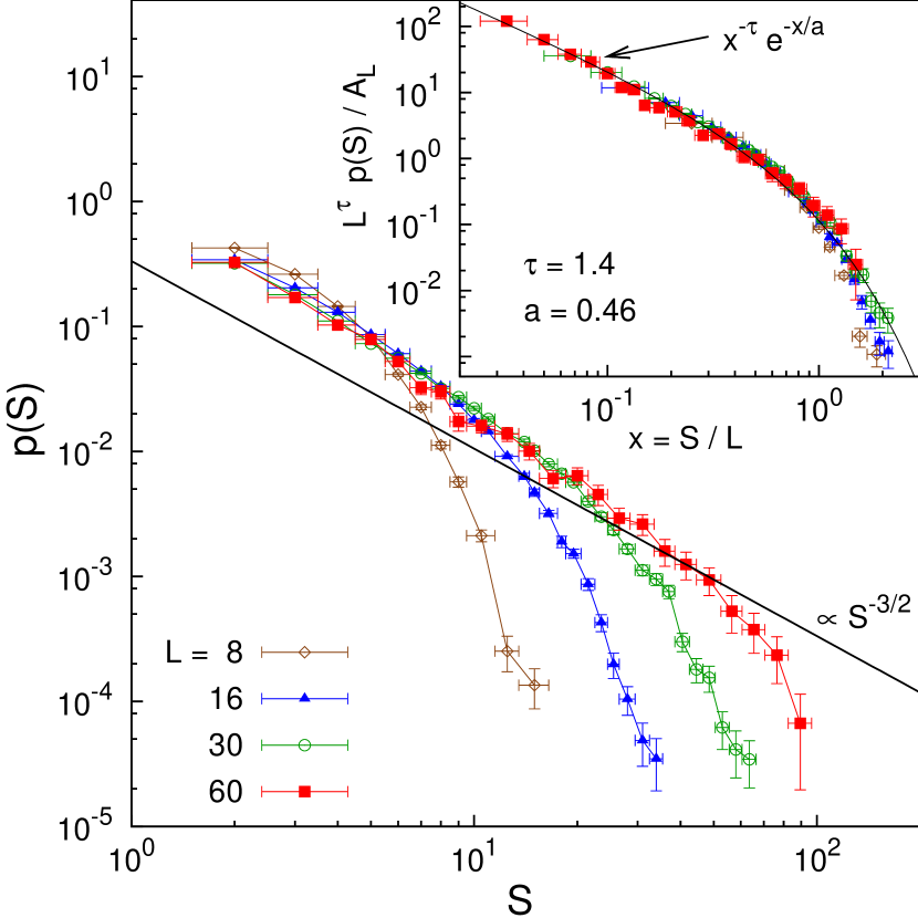
Figure 1: (Color online) Size distribution of the avalanches triggered by an electron displacement and evolved with the $\xi=\infty$ dynamics in 3D, for $W=2$, $K=1/2$. $p(S)$ is obtained from ($90k,48k,29k,2.1k$) samples for $L=(8,16,30,60)$. The initial displacement is the hop of minimal energy that destabilizes at least another pair. Inset: scaling plot of the same data, according to Eq.(2), with $A_{L}$ fixed by normalization.

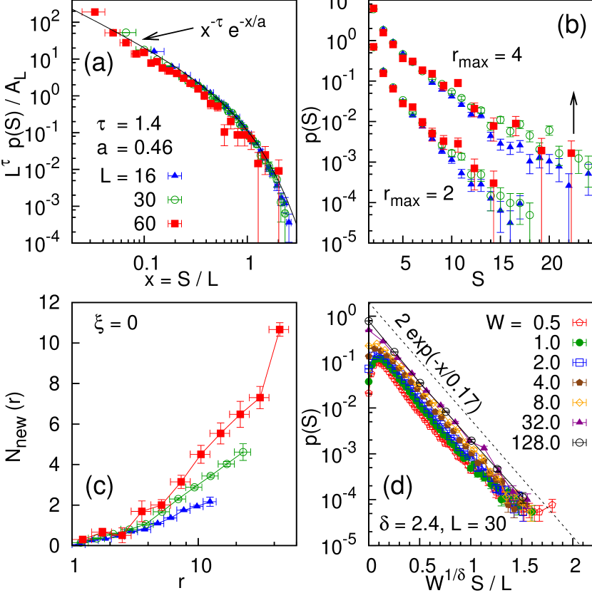
Figure 2: (Color online) (a) Same as the inset of Fig.1 but for the $\xi=0$ dynamics. The initial displacement is the hop of length $r_{ij}=1$ with the smallest energy, which is never allowed to relax back, so the final state is not necessarily metastable. This slight difference from the protocol of Fig.1 is unimportant. (b) Same as Fig.1 but for the $\xi=0$ dynamics with bounded hopping length $r\leq r_{max}$. (c) Average number of pairs destabilized after a hop of length $r$ for different system sizes. Protocol and symbols are as in panel (a). (d) Rescaled size distribution for injection avalanches in 3D evolved with $\xi=\infty$, for different disorder strength $W$, $L=30$, and $K$ in the range $[\frac{1}{2}-\frac{1}{\sqrt{N}},\frac{1}{2}+\frac{1}{\sqrt{N}}]$.

Before addressing the origin of the scale-free behavior, it is useful to analyze the elementary excitations in the avalanches. The energy change due to a hop $i\to j$ is $\omega_{ij}=\varepsilon_{j}-\varepsilon_{i}-e^{2}/r_{ij}$ where $\varepsilon_{i}=e^{2}\sum_{j\neq i}(n_{j}-K)/r_{ij}+\varphi_{i}$ is the energy required to add an electron at site $i$, leaving the rest of the system unchanged. The pairs destabilized in the avalanche are “soft”, with length $r_{ij}$ comparable to $e^{2}/|\varepsilon_{j}-\varepsilon_{i}|$. We find that most are already soft in the initial state (for example, the fraction of hops for which $\omega_{ij}>0.1$ in the initial state is $0.27,0.17,0.12$ for $L=16,30,60$). Thus, the avalanche involves only a small fraction of the sites, as most pairs are “hard”. Efros and Shklovskii argued that $g(\varepsilon)=\langle\delta(\varepsilon_{i}-\varepsilon)\rangle$ vanishes as $|\varepsilon-\mu|^{\delta}$ for $\varepsilon\to\mu$, with $\delta\geq d-1$ ES75 , forming a Coulomb gap of width $\Delta\sim W^{-1/\delta}$. This was confirmed in numerical computations that give $\delta\simeq 2.4\div 2.7$ in three dimensions acre ; mobius , possibly with a crossover to exponential behavior at very low energies baranovski80 ; skinner , and $\delta\simeq 1.0\div 1.2$ in two dimensions mobius ; li ; unpublished . The vast majority of soft pairs are thus dipoles formed by two hard sites with $|\varepsilon_{i,j}-\mu|>\Delta$, with typical length $r_{ij}\simeq r_{0}=e^{2}/\Delta$. Long soft pairs with $r_{ij}\gg r_{0}$ involve sites inside the Coulomb gap ($|\varepsilon_{i,j}-\mu|\ll\Delta$) and thus are much rarer. Neglecting electron-hole correlations, the pair DOS was estimated to behave as $(\omega+1/r)^{2\delta+1}$ for $r\gg r_{0}$ and $\omega\ll\Delta$ baranovski80 . We find that the length distribution of the hops performed during an avalanche decays as $r^{-5.3}$ in 3D, as shown in Fig.S2 of the Supplemental Material Supp , in fairly good agreement with this estimate. The preponderance of short hops even in the $\xi=\infty$ dynamics explains why $p(S)$ maintains an almost identical shape if we let the avalanches evolve with the $\xi=0$ dynamics instead, as shown in Fig.2a.

Let us now turn to injection avalanches, created by adding an extra electron at the empty site with the smallest $\varepsilon_{i}>0$, and simultaneously incrementing the background charge $K$ by $1/N$, to preserve neutrality and avoid the infinite energy required to charge the periodic lattice. Unlike in displacement avalanches, $p(S)$ now has a maximum (Fig.3), which can be understood at mean-field level if we assume that the dipoles destabilized by the initial injection are uncorrelated and thus their number $M$ is Poisson distributed. Then $p(S=0)=e^{-\langle M\rangle}$, and $\langle M\rangle$ can be estimated by counting the pairs with energy smaller than the charge-dipole interaction,

$$\langle M\rangle\simeq\int_{a}^{L}dr\,r^{d-1}\int_{0}^{\frac{e^{2}r_{0}}{r^{2}}}d\omega\Phi(\omega)\simeq r_{0}e^{2}g_{0}L^{d-2}\,,$$ (3)

where the total pair DOS, $\Phi(\omega)=\langle\delta(\omega_{ij}-\omega)\rangle$, for $\omega\ll\Delta$ is of order of the bare single-particle DOS, $g_{0}=e^{2}/(a^{d}W)$ (apart from logarithmic corrections in 3D) baranovski80 . Thus $\langle M\rangle\propto LW^{(1-\delta)/\delta}$ for $d=3$ and $p(S=0)$ decreases exponentially in $L$, consistent with the data in Fig.3. As shown in the inset of Fig.3, the exponential cutoff in the tail of $p(S)$ increases linearly with $L$ as in Eq.(2), with $\tau=1.5(1)$.

Since dipoles are separated from each other by a distance much larger than $r_{0}$, at zero temperature $r_{0}$ and $L$ are the only length scales in avalanches dominated by dipoles. Hence the cutoff, in both types of avalanches, should depend on $L$ via the ratio $L/r_{0}$, a scale invariance stemming entirely from the Coulomb gap. We confirm this prediction by plotting $p(S)$ against $S/(LW^{-1/\delta})$ in Fig.2d: the tails for all values of $W$ (away from the charge-ordered phase gp ) collapse onto the same slope for $\delta=2.4$, in excellent agreement with an independent estimate of $\delta$ from the shape of the Coulomb gap acre . In injection avalanches, $\langle M\rangle$ sets an additional characteristic scale in $p(S)$ that also diverges linearly in $L$, but does not scale with $r_{0}$ since it depends on the charge-dipole rather than the dipole-dipole interaction. We argue later that, as a consequence, $p(S)$ does not develop a power-law tail for $L\to\infty$.

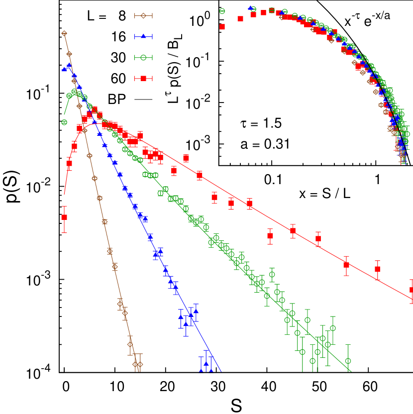
Figure 3: (Color online) Same as Fig.1 but for avalanches triggered by injection. The same samples as in Fig.1 were used. The lines in the main figure represent the best fit, for each value of $L$, to branching process analytical result, Eq.(S11) of the Supplementary Material Supp . In the inset, $B_{L}$ is fixed by normalization, see Eq.(S12) in Ref.Supp .

In 2D, we find that in both displacement and injection avalanches the tail of $p(S)$ is well fitted by Eq.(2), but with a cutoff diverging logarithmically in $L$ (see Fig.S5 and S6 in Supp ). Moreover, for injection avalanches $p(S=0)$ decreases with $L$ much more slowly than in 3D, in agreement with the estimate $\langle M\rangle\propto W^{(1-\delta)/\delta}\log(L/a)$ that follows from Eq.(3).

What is the origin of large avalanches? An argument of Müller and Wyart MW , adapted to the electron glass (see Supp , Section B), predicts that if single electrons can be exchanged with a reservoir from anywhere in the bulk, the mean net number of electrons exchanged during an injection avalanche diverges as $\Delta N_{e}\sim N^{\delta/(1+\delta)}/W$. Hence $\langle S\rangle\geq L^{d-1}$, as follows from $\delta\geq d-1$ and $S\geq\Delta N_{e}$. As observed in Ref.MW , this dynamics is not realistic (in a real system exchanges can only occur at the sample leads), but bulk single-site exchanges are essential for their argument, which holds also if hops between sites are not allowed, since the single-site exchanges suffice to create a Coulomb gap with $\delta\geq d-1$ foot .

The argument of Ref.MW does not apply to injection avalanches under the particle-conserving dynamics considered here, nor to displacement avalanches with or without single-site exchanges. A key observation to understand particle-conserving large avalanches is that long hops, even if rare, are necessary to sustain them. To see this, we modified the $\xi=0$ dynamics by imposing a maximum allowed hopping length $r_{max}$ independent of $L$, and found that the exponential cutoff $S_{c}$ now does not change with $L$, as shown in Fig.2b for displacement avalanches (similar data were obtained in Ref.andresen ). This agrees with the converse of the argument of Ref.MW , which shows that in the absence of a pseudogap the mean avalanche size remains finite. In fact, the only active excitations are now dipoles with $e^{2}r_{0}^{2}/r^{3}$ interaction that do not have a power-law pseudogap. If however we set $r_{max}=L/10$, the cutoff in $p(S)$ becomes again proportional to $L$ (see Fig.S1 in Supp ). The importance of long hops stems from their larger destabilizing effect, shown in Fig.2c, as they act as single-site excitations near the two sites involved, and are more likely to affect regions still untouched by the avalanche.

Motivated by the closeness of $\tau$ to the mean-field value $3/2$ RFIM , we model the avalanches as a branching process, assuming that every hop creates a random number $X$ of subsequent hops with mean $\langle X\rangle=\lambda$. Then, displacement avalanches are described by the well-known Galton-Watson (GW) process Harris : if $\lambda>1$, “explosive” avalanches with $S=O(N)$ occur with finite probability; if $\lambda<1$, one has $\langle S\rangle=(1-\lambda)^{-1}$ and $p(S)$ decays as in Eq.(2) with $\tau=3/2$, with a cutoff diverging as $S_{c}\sim\langle X^{2}\rangle/(1-\lambda)^{2}$ as $\lambda\to 1^{-}$ Harris ; Fisher . Assuming that $X$ is Poisson distributed, $S_{c}$ is a function of $\lambda$ only, and from the fit $S_{c}=0.46L$ in Fig.2 we obtain an effective $L$-dependent $\lambda$ that tends to one for $L\to\infty$ and agrees well, for each $L$, with the mean $\langle X\rangle$ measured by reconstructing the tree of events in each avalanche Supp .

We model injection avalanche as the compound of $M$ independent “sub-avalanches”, each triggered by the relaxation of one the dipoles destabilized by the injection. Hence $S=\sum_{m=1}^{M}S_{m}$, where $S_{m}$ is the size of a sub-avalanche. Assuming that the tail of the distribution of $S_{m}$ has the form in Eq.(2), we have $\langle S\rangle\sim\langle M\rangle S_{c}^{2-\tau}$, and thus Eqs.(2) and (3) imply $\langle S\rangle\sim L^{3-\tau}/W^{(\delta+1-\tau)/\delta}$ in 3D, in agreement with our numerical data (not shown). This differs from the scaling of $\langle S\rangle$ with $L$ and $W$ in the non particle-conserving dynamics, mentioned earlier. Assuming that the sub-avalanches are GW processes and $X$, $M$ are Poisson distributed (as supported by our data Supp ), using a generating function method we obtain an analytical expression for $p(S)$ (Eq.(S11) in Ref.Supp ) parametrized by $\langle M\rangle$ and $\lambda$, which for $S\gg\langle M\rangle$ has the asymptotic form $p(S)\sim\langle M\rangle S^{-3/2}\exp(-S/S_{c}(\lambda))$ with the same dependence $S_{c}(\lambda)$ as in diplacement avalanches. The full analytical expression fits very well our data, as shown in Fig.3. The fits are consistent with a linear scaling of $\langle M\rangle$ and $S_{c}(\lambda)$ in $L$, and agree fairly well for each $L$ with the values of $\langle M\rangle$ and $\lambda$ that obtained from the avalanche tree reconstruction Supp . We stress that the analytical expression for $p(S)$ does not have a power-law tail in the thermodynamic limit since the position of its maximum $S^{*}$ increases with $L$ faster than $S_{c}$ does ($S^{*}/S_{c}\sim L^{1/2}$). This implies that the mean $\langle S\rangle$ is not dominated by rare events, unlike in displacement avalanches, and it explains why the scaled data in the inset of Fig.3 do not show a region with constant slope. We thus have crackling (diverging mean avalanche size) without a power-law distribution. Further details and tests of the branching process model are discussed in Ref.Supp . Despite neglecting the correlations between hops, it reproduces remarkably well the avalanche statistics, suggesting that the system self-organizes to reach the critical point $\lambda=1$. Finding a dynamical explanation of how it does so is a challenging task.

To conclude, our results show that, due to a combination of long-range interaction and long hops, electron glasses displays a self-organized crackling that is qualitatively different from that of the SK model, and is well captured by a mean-field description. To assess the experimental implications of these results, one need to address the time scales of the avalanches as well as the role of temperature and multi-electron transitions. The typical length $r_{typ}$ of thermally activated hops should act as a soft cutoff on the hopping length, and thus on avalanche sizes. Based on the percolation approach to variable-range hopping for the model considered here ESbook , we estimate example that large avalanches could be observable at reasonable time scales at low temperatures. It is likely that multi-electron transitions will contribute significantly to the relaxation before reaching these time scales, as observed in 2D simulations bergli , speeding up the approach to equilibrium, which should shrink further the avalanches. To quantify the impact of such transitions remains a much debated problem Somoza2006 ; Pollak2018 . It would be interesting to search for large rearrangements in disordered insulators in charging experiments Orihuela , or via their effect on the percolating paths in conduction experiments Ovadyahu2014 .

We thank Markus Müller for discussions. This work is supported by AGAUR (2014SGR1379) and MINECO (FIS2015-71582-C2-2-P). We thankfully acknowledge the computer resources at RES-BSC.

Supplemental material: Avalanches in the Relaxation Dynamics of Electron Glasses

Appendix A A. Additional details for simulations in three dimensions

Fig.S1 shows the size distribution of displacement avalanches under the $\xi=0$ dynamics, restricting the hopping length to $r\leq r_{max}=L/10$. In this case, the exponential cutoff increases with the linear system size $L$, unlike in the case of constant $r_{max}$ shown in Fig.2b of the main text, in which the cutoff is independent of $L$.

The length distribution of the hops taking place during a displacement avalanche is shown in Fig.S2. The data up to $r\simeq 10$ lattice spacings are consistent with the power-law decay of the distribution as $\approx 1/r^{2\delta+1}$, in agreement with a mean-field argument based on the Coulomb gap baranovski80 for the DOS of electron-hole pairs. The deviation at large $r$ is a finite-size effect.

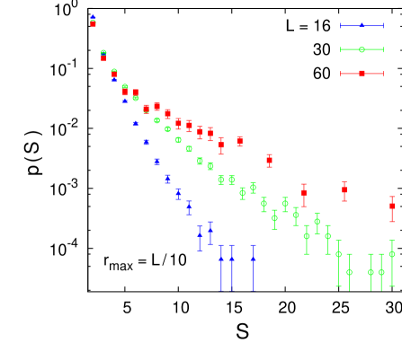
Figure S1: Size distribution of avalanches triggered by an electron displacement and evolved with the $\xi=0$ dynamics in 3D with hopping length restricted to $r\leq r_{max}=L/10$, for $W=2$, $K=1/2$.

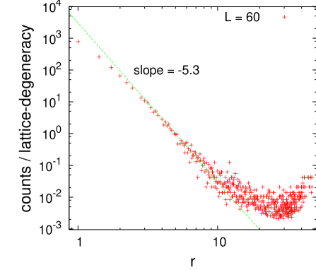
Figure S2: Unnormalized distribution of the length of the hops taking place during the course of avalanches triggered by an electron displacement. The quantity displayed is the number of hops of length $r$, divided the lattice degeneracy (i.e. the number of lattice sites at distance $r$ from a given site, in a periodic cubic lattice of size $L=60$.)

Appendix B B. Mean avalanche size for non-particle-conserving dynamics

We reproduce here the argument of Müller and Wyart MW , adapted to injection avalanches in the electron glass. The argument assumes a non particle-conserving dynamics in which single electrons can be added or removed at any site. In addition, particle-conserving moves, such as single-electron hops, can be allowed but are not necessary for the following argument.

Consider avalanches created by raising the chemical potential $\mu$ quasistatically until one site becomes unstable, which is equivalent to adding an electron at the softest site in our protocol. We assume that the dynamics is such that after each avalanche a Coulomb gap is restored, so that the single-particle DOS behaves as $g(\epsilon)=c_{d}|\epsilon-\mu|^{\delta}$ for small $|\epsilon-\mu|$. As mentioned in the main text, single-site exchanges are sufficient to restore a Coulomb gap with $\delta\geq d-1$. Then, at each electron injection the chemical potential $\mu$ is shifted by an amount $\Delta\mu$ such that $Na^{d}\int_{\mu}^{\mu+\Delta\mu}g(\epsilon)d\epsilon$ is of order one, i.e. $\Delta\mu\sim(c_{d}a^{d}N)^{-1/(\delta+1)}$. Provided neutrality is maintained by changing the compensating charge $K$ at each particle exchange, the inverse compressibility $\chi(\mu)^{-1}=d\mu/d\langle K\rangle$ remains finite. Consider now successive avalanches created by sweeping quasistatically $\mu$ in a range $[-\mu_{max},\mu_{max}]$, with $\mu_{max}$ of order of the disorder strength $W$ so that $K(\mu_{max})\simeq 1$ (and $K(-\mu_{max})\simeq 0$). The average net number of electrons entering the system at each avalanche is $\Delta N_{e}=N\langle\chi(\mu)\rangle\Delta\mu$, and since $\langle\chi(\mu)\rangle\simeq 1/W$, we obtain

$$\Delta N_{e}\simeq N^{\delta/(1+\delta)}/[W(c_{d}a^{d})^{1/(\delta+1)}]$$ (S1)

Two observations not included in the argument of Ref.MW, are in order. First, if the charge is not compensated by changing $K$, then the system is incompressible ($\chi(\mu)^{-1}$ diverges with $L$), so the above argument does not hold. Second, the finite system size modifies the shape of the Coulomb gap for $|\epsilon-\mu|$ below an energy of order $e^{2}/L$, and the above argument needs to be modified accordingly. Because of this finite-size effect, $\Delta\mu\sim e^{2}/L$, with a proportionality constant that depends on the boundary conditions. Thus Eq.(S1) gets modified as $\Delta N_{e}\simeq e^{2}L^{d-1}/(Wa^{d})$. This is the same form taken by Eq.(S1) if the Efros-Shklovskii bound is saturated, i.e. $\delta=d-1$ (in which case $c_{d}$ is proportional to $e^{-2d}$), which was found numerically to be the case when the only moves allowed are the particle exchanges with the reservoir unpublished .

Appendix C C. Branching process model

We model injection avalanches as a compound of a random number $M$ of independent sub-avalanches, each described by a Galton-Watson (GW) branching process Harris . The total avalanche size is then

$$S=\sum_{m=1}^{M}Y_{m}$$ (S2)

in which $Y_{m}$ is the size (namely, the number of branches of the GW process) of the $m$-th sub-avalanche ($Y_{m}$ is called $S_{m}$ in the main text. In this Section, we change notation to avoid confusion with $S$.) $M$ is the random number of pairs that were destabilized by the initial injection and that later relaxed, with $\langle M\rangle=\rho_{L}$.

Each hop is assumed to create $X$ subsequent hops with probability $p(X)$, with $\langle X\rangle=\lambda_{L}$, where we allow the mean to depend on $L$ to account for finite-size effects. The sub-avalanche size is thus $Y_{m}=\sum_{k=1}^{\infty}Z_{k}$, where $Z_{k}$ is the number of hops at generation $k$ of the branching tree, which satisfies the recursion relation

$$Z_{1}=1,\qquad Z_{n+1}=\sum_{i=1}^{Z_{n}}X_{i}$$ (S3)

where the $X_{i}$ are independent, identically distributed (i.i.d.) copies of $X$.

The probability distributions of $Y$, denoting with this symbol any of the i.i.d. variables $Y_{m}$, and of $S$ can be determined with generating function methods. It is easy to show (see e.g. Ref.Harris, ) that the generating functions of $Y$ and $S$, $g_{Y}(t)=\langle t^{Y}\rangle$ and $g_{S}(t)=\langle t^{S}\rangle$, satisfy the equations

$$g_{Y}(t)=tg_{X}(g_{Y}(t))$$ (S4)

$$g_{S}(t)=g_{M}(g_{Y}(t))$$ (S5)

where $g_{X}(t)=\langle t^{X}\rangle$ and $g_{M}(u)=\langle u^{M}\rangle$ are the generating functions of $X$ and $M$, respectively.

By expanding $g_{Y}(t)$ in $t$ one immediately obtains $\langle Y\rangle=(1-\lambda_{L})^{-1}$. From Eq.(S4) one can also obtain Harris the asymptotic behavior of $p(Y)$ at large $Y$,

$$p(Y)\sim Y^{-3/2}e^{-Y/S_{c}},$$ (S6)

where the cutoff diverges as $S_{c}\sim\langle X^{2}\rangle/(1-\lambda_{L})^{2}$ for $\lambda_{L}\to 1^{-}$, as follows from the general expression given by Harris Harris for $S_{c}$. The same result was also obtained by Fisher with a similar method Fisher .

In the special case in which $X$ is Poisson distributed, we have $g_{X}(t)=\exp(\lambda_{L}(x-1))$ and Eq.(S4) can be solved explicitly, giving

$$g_{Y}(t)=-\frac{1}{\lambda_{L}}W\left[-\lambda_{L}\exp(-\lambda_{L})t\right]\,,$$ (S7)

where $W(x)$ is the Lambert $W$ function, with series representation $W(x)=\sum_{n=1}^{\infty}(-n)^{n-1}x^{n}/n!$ for $|x|<\exp(1)$. This immediately gives

$$p(Y)=\frac{{(\lambda_{L}Y)}^{Y-1}}{Y!}\exp[-\lambda_{L}Y]\,.$$ (S8)

The asymptotic behavior of Eq.(S8) for large $Y$ is

$$p(Y)\sim\frac{1}{\sqrt{2\pi\lambda_{L}^{2}}}Y^{-3/2}\exp[-Y/S_{c}]$$ (S9)

with

$$S_{c}=(\lambda_{L}-1-\log\lambda_{L})^{-1}.$$ (S10)

If $M$ is also Poisson-distributed with mean $\rho_{L}$, by expanding Eq.(S5) around $t=0$ we obtain

$$p(S)=\frac{\rho_{L}(\lambda_{L}S+\rho_{L})^{S-1}}{S!}\exp[-(\lambda_{L}S+\rho_{L})]\,.$$ (S11)

Eq.(S11) fits very well the data for injection avalanches, as shown in Fig.3 of the main text. The fit parameters $\rho_{L}$ and $\lambda_{L}$ for each $L$ are consistent with linear scaling $\rho_{L}=0.09(1)L$ and $S_{c}=0.31(4)L$, for $S_{c}$ given by Eq.(S10).

For $S\ll\rho_{L}$, $p(S)$ in Eq.(S11) tends to a Poisson distribution, while for $S\gg\rho_{L}$ it has the form of a power law with exponential cutoff

$$p(S)\sim B_{L}\,S^{-3/2}\exp{\left[-S/S_{c}\right]}\,.$$ (S12)

where $B_{L}=\rho_{L}\exp(\rho_{L}/\lambda_{L}-\rho_{L})(2\pi\lambda_{L}^{2})^{-1/2}$. A scaling plot according to this form is shown in Fig.3 of the main text.

The function $p(S)$ in Eq.(S11) presents a maximum at $S=S^{*}$. To estimate $S^{*}$, we solve $d\log p(S)/dS=0$ using Stirling’s approximation, which gives

$$\log\frac{\lambda_{L}S^{*}+\rho_{L}}{S^{*}}+\frac{\lambda_{L}(S^{*}-1)}{\lambda_{L}S^{*}+\rho_{L}}-\lambda_{L}-\frac{1}{2S^{*}}=0\,.$$ (S13)

To leading order we then have $S^{*}=\rho_{L}/(1-\lambda_{L})=\langle S\rangle$ and expanding in the small parameter $x=[\rho_{L}(1-\lambda_{L})]^{-1}\sim\sqrt{S_{c}}/\rho_{L}\sim 1/\sqrt{L}$ we obtain the corrections

$$S^{*}=\langle S\rangle(1-\lambda_{L}x-\frac{\lambda_{L}}{2}x^{2}+O(x^{3}))\,.$$ (S14)

The important point to note is that in 3D, since $\rho_{L}\propto W^{1/\delta-1}L$ and $S_{c}\propto LW^{-1/\delta}$, as discussed in the main text, and since $\langle S\rangle\sim\rho_{L}S_{c}^{1/2}$, the ratio $S^{*}/S_{c}$ is proportional to $L^{1/2}/W^{\frac{3}{2\delta}-1}$ and thus diverges for large $L$. Hence, the power law behavior $p(S)\sim S^{-3/2}$ is never observed, since the position of the maximum is increasingly larger than the cutoff. A similar estimate in 2D, noting that $\rho_{L}$ and $S_{c}$ both increase logarithmically with $L$, gives $S^{*}/S_{c}\sim(\log L)^{1/2}$.

Appendix D D. Tests of the branching process model

4.1 D.1. Procedure

In order to test the branching process description of the avalanches, we reconstructed the genealogical tree of each individual injection avalanche by keeping track of the offspring of each hop, as described in the following.

Let $J_{1},J_{2},\dots,J_{S}$ be the hops taking place in the course of an avalanche of size $S$, in the order they occurred. We call $\mathfrak{U}_{1}$ the set of electron-hole pairs that become unstable after the initial electron injection, and $\mathfrak{U}_{i}$, $i>1$ the set of pairs that are unstable after hop $J_{i-1}$ and before hop $J_{i}$ (regardless of when they became unstable).

We call progeny of a hop $J_{i}$ the set of hops $J_{l}$ with $l>i$ such that $J_{l}\in\mathfrak{U}_{k}$ for all $k=i+1,\dots,l$ and $J_{l}\notin\mathfrak{U}_{i}$, namely those hops that relaxed pairs that were destabilized by $J_{i}$ and remained unstable at all times until they relaxed. (The progeny does not include pairs that, after being destabilized by $J_{i}$, are stabilized again by subsequent hops without relaxing.) We call $X_{i}$ the size of the progeny of $J_{i}$ and measure its distribution $p(X)=\langle S^{-1}\sum_{i=1}^{S}\delta_{X_{i},X}\rangle$ by averaging over all the avalanches (one avalanche per disorder realization at $K=1/2$).

The first generation of an avalanche is the set of hops $J_{i}$ such that $J_{i}\in\mathfrak{U}_{k}$ for all $k=1,\dots,i$, namely those hops that relaxed pairs that were destabilized by the initial injection and remained unstable at all times until they relaxed. We call $M$ the number of first-generation hops, and denote by $p(M)$ its distribution, again estimated by averaging over all avalanches.

The $k$-th generation of the avalanche is the set of hops that belong to the progeny of a hop that itself belongs to generation $k-1$. Finally, we call sub-avalanche each of the $M$ first generation hops together with its progeny (i.e. the subtree arising from it).

4.2 D.2. Statistics of the first generation

The top two panels of Fig. S3 summarize the statistics of $M$ obtained using the above procedure for $W=2$. Panel (a) shows that the cumulative distribution function of $M$ for different system sizes agrees reasonably well with a Poisson distribution of mean $\rho_{L}$ equal to the measured mean $\langle M\rangle$. The deviation from the Poisson distribution reflects the correlations between soft electron-hole pairs, and can be quantified by the relative difference between $\rho_{L}$ and the measured variance of $M$, both shown in the panel (b), which is around 30$\%$.

The mean grows approximately linearly with $L$, the best fit giving $\rho_{L}=0.068(6)L$, and is not far from the estimate $\rho_{L}$ obtained from the two-parameter fits of Eq.(S11) to $p(S)$ for injection avalanches, also shown in Fig. S3 (b), which is fitted by $\rho_{L}=0.09(1)L$ as discussed in Section C. The linear increase of $\rho_{L}$ with $L$ agrees with the mean-field estimate in Eq.(3) of the main text, which assumes a constant pair DOS. In fact, it is known that at small $\omega$ the pair DOS decreases logarithmically baranovski80 , which produces logarithmic corrections to the linear dependence of $\rho_{L}$ on $L$. Including these corrections, we reproduce the deviation from linearity observed in Fig. S3.

4.3 D.3. Statistics of the branching ratio

The statistics of $X$ for $W=2$ are summarized in the bottom panels of Fig. S3. The distribution $p(X)$ obtained by averaging over all hops (not shown) shows a dependence on the system size. In particular, as shown in the panel (d), its mean $\lambda_{L}=\langle X\rangle$ increases with $L$, giving a linear increase $S_{c}=0.45(9)L$ if we define $S_{c}$ as in Eq.(S10). This agrees very well with the observed linear increase of the cutoff of $p(S)$ for displacement avalanches, which can be fitted to $S_{c}=0.46(8)L$ (Fig.1 of the main text), and fairly well with the analogous fit for injection avalanches which gives $S_{c}=0.31(4)L$ (Fig.3 of the main text).

We ascribe the dependence of $p(X)$ on the system size to the fact that when an avalanche reaches the boundary of the system and enters again from the “opposite side”, it revisits regions already affected by the avalanche, which are more stable and thus tend to reduce $\langle X\rangle$. To filter out this finite-size effect and test the validity of the branching process description, we also estimated $p(X)$ including only “mid-generations” hops, namely hops that a) belong to sub-avalanches that are at least six generations deep and b) are within the central $40\%$ of the generations of the sub-avalanche to which they belong. As shown in Fig. S3 (c) the distribution measured in this way is relatively independent of $L$. For the larger system sizes $L=60,100$, for which the mid-generation protocol should filter out finite-size effects more effectively, $p(X)$ is well described by a Poisson distribution of mean unity, in agreement with the assumption of a critical GW process.

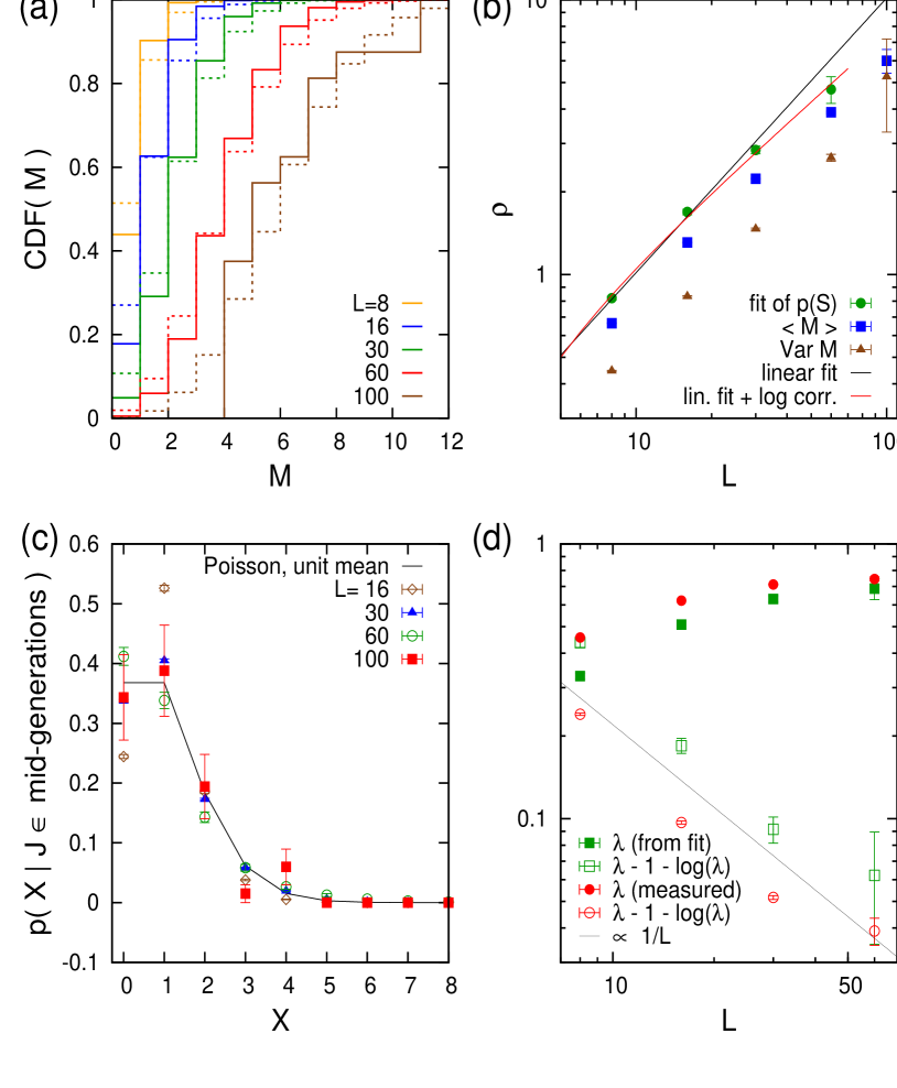
Figure S3: Statistics of the reconstructed avalanche tree for $W=2$. (a) The cumulative distribution function of the number $M$ of first-generation hops (continuous lines) is compared with a Poisson distribution of mean $\rho_{L}=\langle M\rangle$ (dashed lines) for different sizes $L$. (b) $\langle M\rangle$ (blue squares) compared to the value of $\rho_{L}$ (green circles) obtained by fitting Eq.(S11) to the size distribution of injection avalanches in 3D, shown in Fig.3 of the main text. The two values are fairly close, supporting the branching process description, and increase linearly with $L$, possibly with some logarithmic corrections. Also shown is the variance of $M$ (brown triangles), which differs from the mean, highlighting a deviation from Poisson statistics. (c) The distribution of the number of offspring $X$, measured in mid-generations is approximately independent of $L$ and well described by a Poisson distribution with mean $\lambda_{L}=1$. (d) The value of $\lambda_{L}$ obtained by fitting Eq.(S11) to the data of Fig.3 of the main text is compared with $\lambda_{L}=\langle X\rangle$ measured including all generations.

4.4 D.4. Size distribution of sub-avalanches

Fig.S4 shows the size distribution of the sub-avalanches, defined as explained in paragraph D.1. The shape of $p(S)$ is practically indistinguishable from that of displacement avalanches shown in Fig.1 of the main text, supporting our assumption that injection avalanches are well approximated by the compound of $M$ displacement avalanches.

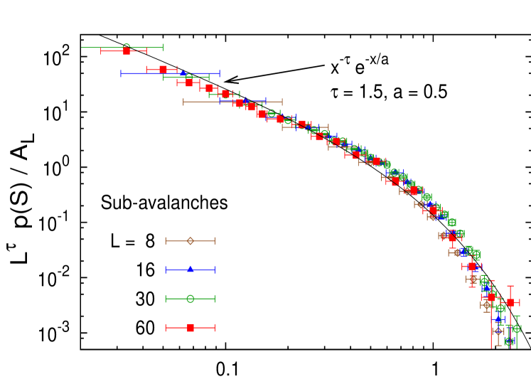
Figure S4: Size distribution of the sub-avalanches of injection avalanches, obtained by identifying the progeny of the hops that were destabilized by the electron injection.

Appendix E E. Avalanches in two dimensions

We report here the results of our simulations in two dimensions, which followed the same protocol described in the main text for three dimensional simulations. Fig.S5 shows the size distribution of displacement avalanches under the $\xi=\infty$ dynamics. The data can be fitted by Eq.(2) of the main text with $\tau=1.5$, similarly to the results in 3D (Fig.1 of the main text). However in 2D the cutoff increases logarithmically with $L$ instead of linearly, as shown by the scaling plot in the figure inset.

Fig.S6 shows the size distribution of injection avalanches in 2D under the same dynamics. As in displacement avalanches, the cutoff grows with $L$ much more slowly than in 3D (see Fig.3 of the main text), and is consistent with a logarithmic dependence. $p(S=0)$ decreases much more slowly with $L$ than in 3D, in agreement with the estimate $p(S=0)=e^{-\langle M\rangle}$ and with a logarithmic growth of $\langle M\rangle$ with $L$ implied by the mean-field estimate in Eq.(3) of the main text. By fitting Eq.(S11) to the data in Fig. S6, we determine the parameters $\lambda_{L}$ and $\rho_{L}$. As shown in the figure inset, the fitted parameters are consistent with a logarithmic growth $\rho_{L}\propto\log L$ and $S_{c}(\lambda_{L})\propto\log L$.

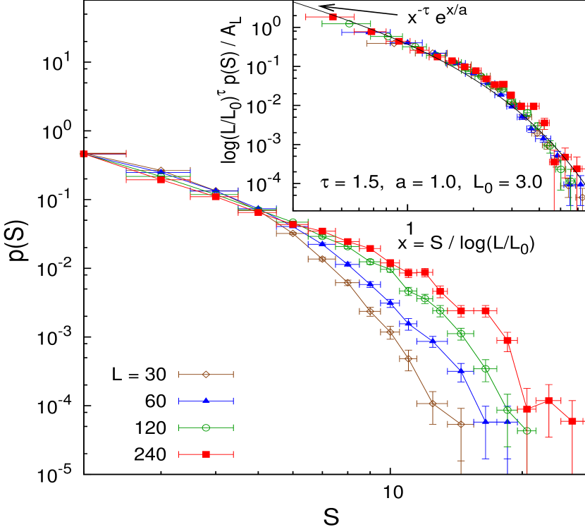
Figure S5: Avalanche size distribution for displacement avalanches in 2D, evolved with the $\xi=\infty$ dynamics, for $W=2$, $K=1/2$, and $L=30,60,120,240$. Inset: rescaling of the data according to Eq.(2) of the main text, with a logarithmic cutoff.

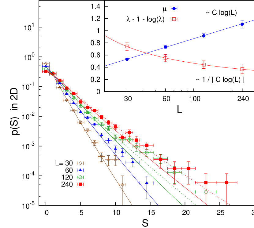
Figure S6: Same as Fig. S5 except that avalanches are triggered by injection. The solid lines are fits to Eq.S11. The inset shows that the $L$-dependence of both fit parameters $\lambda_{L}$ and $\rho_{L}$ is consistent with a logarithmic dependence $S_{c},\rho_{L}\propto\log L$.

References

- (1) B. I. Shklovskii and A. L. Efros. Electronic Properties of Doped Semiconductors (Springer, Berlin, 1984).
- (2) M. Pollak, M. Ortuño, A. Frydman, The electron glass (Cambridge University Press, 2013).
- (3) M. Palassini, Contrib. Sci. 11(2), 163 (2015).
- (4) A. L. Efros and B. I. Shklovskii, J. Phys. C 8, L49 (1975).
- (5) M. Pollak, Discuss. Faraday Soc. 50, 13 (1970).
- (6) J.H. Davies, P.A. Lee, T.M. Rice, Phys. Rev. Lett. 49, 758 (1982); Phys. Rev. B 29, 4260 (1984).
- (7) J. R. L. de Almeida and D. J. Thouless, J. Phys. A 11, 983 (1978).
- (8) D. Sherrington and S. Kirkpatrick, Phys. Rev. Lett. 35, 1792 (1975). S. Kirkpatrick and D. Sherrington, Phys. Rev. B 17, 4384 (1978).
- (9) M. Müller and L. B. Ioffe, Phys. Rev. Lett. 93 (2004); S. Pankov and V. Dobrosavljević, Phys. Rev. Lett. 94, 046402 (2005); M. Müller and S. Pankov, Phys. Rev. B 75, 144201 (2007).
- (10) A. A. Pastor and V. Dobrosavljević, Phys. Rev. Lett. 83 4642 (1999).
- (11) M. Goethe and M. Palassini, Phys. Rev. Lett. 103, 045702 (2009).
- (12) B. Surer, H.G. Katzgraber, G.T. Zimanyi, B.A. Allgood, and G. Blatter, Phys. Rev. Lett. 102, 067205 (2009).
- (13) M. Ben-Chorin, Z. Ovadyahu, M. Pollak, Phys. Rev. B 48, 15025 (1993).
- (14) T. Grenet, J. Delahaye, M. Sabra, F. Gay, Eur. Phys. J B 56, 183 (2008).
- (15) T. Havdala, A. Eisenbach, A. Frydman, Euro Phys. Lett. 98, 67006 (2012).
- (16) Z. Ovadyahu, C. R. Physique 14, 700 (2013).
- (17) R. G. Palmer and C. M. Pond, J. Phys. F: Metal Phys. 9, 1451 (1979).
- (18) F. Pázmándi, G. Zaránd, and G. T. Zimányi, Phys. Rev. Lett. 83, 1034 (1999).
- (19) D.J. Thouless, P.W. Anderson, and R.G. Palmer, Phil. Mag. 35 593 (1977).
- (20) A. A. Pastor, V. Dobrosavljevic, and M. L. Horbach, Phys. Rev. B 66, 014413 (2002).
- (21) S. Boettcher, H.G. Katzgraber, and D. Sherrington, J. Phys. A: Math. Theor. 41, 324007 (2008).
- (22) B. Gonçalves and S. Boettcher, J. Stat. Mech. P01003 (2008).
- (23) J.C. Andresen, Z. Zhu, R.S. Andrist, H.G. Katzgraber, V. Dobrosavljević, and G.T. Zimanyi, Phys. Rev. Lett. 111, 097203 (2013).
- (24) O. Perkovic, K. A. Dahmen, and J. P. Sethna, Phys. Rev. Lett. 75, 4528 (1995); K. Dahmen and J. P. Sethna, Phys. Rev. B 53, 14872 (1996).
- (25) S. Field, J. Witt, F. Nori, and W. S. Ling, 74, 1206 (1995); K. Behnia, C. Capan, D. Mailly, and B. Etienne, Phys. Rev. B 61, 3815 (2000).
- (26) L. Carrillo, L. Mañosa, J. Ortín, A.Planes, and E. Vives, Phys. Rev. Lett. 81, 1889 (1998).
- (27) E.K.H. Salje and K. A. Dahmen, Ann. Rev. of Cond. Matt. Phys. 5, 233 (2014).
- (28) M. Müller and M. Wyart, Ann. Rev. Cond. Matt. Phys. 6, 177 (2015).
- (29) D. Monroe, A. C. Gossard, J. H. English, B. Golding, and W. H. Haemmerle, Phys. Rev. Lett . 59, 1148 (1987).
- (30) Z. Ovadyahu, Phys. Rev. B 90, 054204 (2014).
- (31) M. Palassini and M. Goethe, J. Phys.: Conf. Ser. 376, 012009 (2012).
- (32) A. L. Efros, J. Phys. C 9, 2021 (1976).
- (33) A. Glatz, V. M. Vinokur, J. Bergli, M. Kirkengen, and Y. M. Galperin, J. Stat. Mech. P06006 (2008).
- (34) A. Möbius, M. Richter, and B. Drittler, Phys. Rev. B 45, 11568 (1992).
- (35) S.D. Baranovskii, B.I. Shklovskii, and A.L. Efros, Sov. Phys. JETP 51, 199 (1980).
- (36) A.L. Efros, B. Skinner, and B.I. Shklovskii, Phys. Rev. B 84, 064204 (2011).
- (37) Q. Li and P. Phillips. Phys. Rev. B 49, 10269 (1994).
- (38) M. Goethe and M. Palassini, unpublished.
- (39) See Supplemental Material at [URL will be inserted by publisher] for additional plots, calculation details and numerical tests of the branching process model.
- (40) The number of sites destabilized by an electron exchange is of order if . In order to reach a stable configuration, after the last exchange this number cannot diverge, thus .
- (41) J.C. Andresen, Y. Pramudya, H.G. Katzgraber, C.K. Thomas, G.T. Zimanyi, and V. Dobrosavljević, Phys. Rev. B 93, 094429 (2016).
- (42) T.E. Harris, The Theory of Branching Processes (Springer-Verlag, Berlin 1963).
- (43) D.S. Fisher, Phys. Rep. 301, 113 (1998).
- (44) The percolation approach gives with , with an associated time scale where s ESbook . For and we have . Extrapolating from Fig.S1 Supp and Fig.3, single electrons will trigger avalanches with hops with probability and duration s.
- (45) J. Bergli, A. M. Somoza, and M. Ortuño, Phys. Rev. B 84, 174201 (2011).
- (46) A. M. Somoza, M. Ortuño, and M. Pollak, Phys. Rev. B 73, 045123 (2006).
- (47) M. Pollak, J. Phys.: Condens. Matter 30, 105602 (2018).
- (48) M. F. Orihuela, M. Ortuño, A. M. Somoza, J. Colchero, and E. Palacios-Lidón, T. Grenet and J. Delahaye, Phys. Rev. B 95, 205427 (2017).