Computing a Pessimistic Leader-Follower Equilibrium with Multiple Followers: the Mixed-Pure Case

Abstract

The search problem of computing a leader-follower equilibrium (also referred to as an optimal strategy to commit to) has been widely investigated in the scientific literature in, almost exclusively, the single-follower setting. Although the optimistic and pessimistic versions of the problem, i.e., those where the single follower breaks any ties among multiple equilibria either in favour or against the leader, are solved with different methodologies, both cases allow for efficient, polynomial-time algorithms based on linear programming. The situation is different with multiple followers, where results are only sporadic and depend strictly on the nature of the followers’ game.

In this paper, we investigate the setting of a normal-form game with a single leader and multiple followers who, after observing the leader’s commitment, play a Nash equilibrium. The corresponding search problem, both in the optimistic and pessimistic versions, is known to be not in Poly-APX unless $\textsf{P}=\textsf{NP}$ and exact algorithms are known only for the optimistic case. We focus on the case where the followers play in pure strategies—a restriction that applies to a number of real-world scenarios and which, in principle, makes the problem easier—under the assumption of pessimism (as it is easy to show, the optimistic version of the problem can be straightforwardly solved in polynomial time). After casting this search problem as a pessimistic bilevel programming problem, we show that, with two followers, the problem is NP-hard and, with three or more followers, it is not in Poly-APX unless $\textsf{P}=\textsf{NP}$. This last result matches the inapproximability result which holds for the unrestricted case and shows that, differently from what happens in the optimistic version, hardness in the pessimistic problem is not due to the adoption of mixed strategies. We then show that the problem admits, in the general case, a supremum but not a maximum, and we propose a single-level mathematical programming reformulation which calls for the maximisation of a nonconcave quadratic function over an unbounded nonconvex feasible region defined by linear and quadratic constraints. Since, due to admitting a supremum but not a maximum, only a restricted version of this formulation can be solved to optimality with state-of-the-art methods, we propose an exact ad hoc algorithm, which we also embed within a branch-and-bound scheme, capable of computing the supremum of the problem and, for cases where there is no leader’s strategy where such value is attained, also an $\alpha$-approximate strategy where $\alpha>0$ is an arbitrary additive loss. We conclude the paper by evaluating the scalability of our algorithms via computational experiments on a well-established testbed of game instances.

1 Introduction

In recent years, Leader-Follower (or Stackelberg) Games (LFGs) and their corresponding Leader-Follower Equilibria (LFEs) have attracted a growing interest in many disciplines, including theoretical computer science, artificial intelligence, and operations research. LFGs describe situations where one player (the leader) commits to a strategy and the other players (the followers) first observe the leader’s commitment and, then, decide how to play. In the literature, LFEs are often referred to as optimal strategies (for the leader) to commit to. LFGs encompass a broad array of real-world games. A prominent example is that one of security games, where a defender, acting as a leader, is tasked to allocate scarce resources to protect valuable targets from an attacker, acting as a follower An et al (2011); Kiekintveld et al (2009); Paruchuri et al (2008). Besides the security domain, applications can be found in, among others, interdiction games Caprara et al (2016); Matuschke et al (2017), toll-setting problems Labbé and Violin (2016), and network routing Amaldi et al (2013).

While, to the best of our knowledge, the majority of the game theoretical investigations on the computation of LFEs assumes the presence of a single follower, we address, in this work, the multi-follower case.

When facing an LFG and, in particular, a multi-follower one, two aspects need to be considered: the type of game (induced by the leader’s strategy) the followers play and, in it, how ties among the multiple equilibria which could arise are broken.

As to the nature of the followers’ game, and restricting ourselves to the cases which look more natural, the followers may play hierarchically one at a time, as in a hierarchical Stackelberg game Conitzer and Sandholm (2006), simultaneously and cooperatively Conitzer and Korzhyk (2011), or simultaneously and noncooperatively Basilico et al (2016).

As to breaking ties among multiple equilibria, it is natural to consider two cases: the optimistic one, where the followers end up playing an equilibrium which maximises the leader’s utility, and the pessimistic one, where they end up playing an equilibrium by which the leader’s utility is minimised. Note that we are not assuming, here, that the followers could agree on an optimistic or pessimistic equilibrium in a practical application. Rather, the optimistic and pessimistic cases allow for the computation of the tightest range of values the leader’s utility may take without making any assumptions on which equilibrium the followers would actually end up playing. From this perspective, while an optimistic LFE accounts for the best case for the leader, a pessimistic LFE accounts for the worst case. In this sense, the computation of a pessimistic LFE is paramount in realistic scenarios as, differently from an optimistic one, the former is robust. As we will see, though, this degree of robustness comes at a high computational price, as computing a pessimistic LFE is a much harder task than computing its optimistic counterpart.

1.1 Leader-Follower Nash Equilibria

Throughout the paper, we will focus on the case of normal-form games where, after the leader’s commitment to a strategy, the followers play simultaneously and noncooperatively, reaching a Nash equilibrium. We refer to the corresponding equilibrium as Leader-Follower Nash Equilibrium (LFNE).

In particular, we consider the case where the followers are restricted to pure strategies. This restriction is motivated by some reasons. First, the problem of finding an NE in mixed strategies, a subproblem of that of finding an LFNE, is already hard with two or more players (which clearly implies the hardness of finding an LFNE in mixed strategies)—differently from the problem of computing an NE in pure strategies, which can be solved in polynomial time. Thus, the study of the case where followers play pure strategies does not appear direct and could allow one to characterise more accurately the tractability of the problem. Secondly, many games admit pure-strategy NEs, among which potential games Monderer and Shapley (1996), congestion games Rosenthal (1973), and toll-setting problems Labbé and Violin (2016). The same also holds, with high probability, in many unstructured games (see Subsection 3.3).

1.2 Original Contributions

After briefly pointing out that an optimistic LFNE (with followers restricted to pure strategies) can be computed efficiently (in polynomial time) by a mixture of enumeration and linear programming, we entirerly devote the remainder of the paper to the pessimistic case (with, again, followers restricted to pure strategies). In terms of computational complexity, we show that, differently from the optimistic case, in the pessimistic case the equilibrium-finding problem is NP-hard with two or more followers and not in Poly-APX when the number of followers is three or more unless $\textsf{P}=\textsf{NP}$. To establish these two results, we introduce two reductions, one from Independent Set and the other one from 3-SAT.

After analysing the complexity of the problem, we focus on its algorithmic aspects. First, we formulate the problem as a pessimistic bilevel programming problem with multiple followers. We, then, show how to recast it as a single-level Quadratically Constrained Quadratic Program (QCQP), which we show to be impractical to solve due to admitting a supremum, but not a maximum. We, then, introduce a restriction based on a Mixed-Integer Linear Program (MILP) which, while forsaking optimality, always admits an optimal (restricted) solution. Next, we propose an exact algorithm to compute the value of the supremum of the problem, based on an enumeration scheme which, at each iteration, solves a lexicographic MILP (lex-MILP) where the two objective functions are optimised in sequence. Subsequently, we embed the enumerative algorithm within a branch-and-bound scheme—obtaining an algorithm which is, in practice, much faster. We also extend the algorithm (in both versions) so that, for cases where the supremum is not a maximum, it returns a strategy by which the leader can obtain a utility within an additive loss $\alpha$ with respect to the supremum, for an arbitrarily chosen $\alpha>0$. To conclude, we experimentally evaluate the scalability of our methods over a rich testbed of instances which is standard in game theory.

The status, in terms of complexity and known algorithms, of the problem of computing an LFNE (with followers playing pure or mixed strategies) is summarised in Table 1. The original results we provide in this paper are reported in boldface.

Table 1: Summary of known results for the computation of an LFNE. The entries in boldface correspond to original contributions of this work. The number of players is denoted by $n$.

1.3 Paper Outline

The paper is organised as follows. Previous works are introduced in Section 2. The problem we study is formally stated in Section 3, together with some preliminary results. In Section 4, we present the computational complexity results. Section 5 introduces the single-level reformulation(s) of the problem, while Section 6 describes our exact algorithm (in its two versions). An empirical evaluation of our methods is carried out in Section 7. Section 8 concludes the paper.

2 Previous Works

As we mentioned in Section 1, most of the works on (normal-form) LFGs focus on the single-follower case. In such case, as shown in Conitzer and Sandholm (2006), the follower always plays a pure strategy, except for degenerate games. In the optimistic case, an LFE can be found in polynomial time by solving a Linear Program (LP) for each action of the (single) follower (the algorithm is, thus, a multi-LP). Each LP maximises the expected utility of the leader, subject to a set of constraints imposing that the given follower’s action is a best-response Conitzer and Sandholm (2006). As shown in Conitzer and Korzhyk (2011), all these LPs can be encoded into a single LP—a slight variation of the LP that is used to compute a correlated equilibrium (the solution concept where all the players can exploit a correlation device to coordinate their strategies). Some works study the equilibrium-finding problem (only in the optimistic version) in structured games where the action space is combinatorial. See Basilico et al (2017b) for more references.

For what concerns the pessimistic single-follower case, the authors of von Stengel and Zamir (2010) study the problem of computing the supremum of the leader’s expected utility. They show that, for the latter, it suffices to consider the follower’s actions which constitute a best-response to a full-dimensional region of the leader’s strategy space. The multi-LP algorithm the authors propose solves two LPs per action of the follower, one to verify whether the best-response region for that action is full-dimensional (so to discard it if full-dimensionality does not hold) and a second one to compute the best leader’s strategy within that best-response region. The algorithm runs in polynomial time. While the authors limit their analysis to computing the supremum of the leader’s utility, we remark that such value does not always translate into a strategy that the leader can play as, in the general case where the leader’s utility does not admit a maximum, there is no leader’s strategy giving her a utility equal to the supremum. In such cases, one should rather look for a strategy providing the leader with an expected utility which approximates the value of the supremum. This aspect, which is not addressed in von Stengel and Zamir (2010), will be tackled, on the multi-follower case, by our work.

The multi-follower case, which, to the best of our knowledge, has only been investigated in Basilico et al (2016, 2017a), is computationally much harder than the single-follower case, being, in the general case with the leader and the followers entitled to mixed strategies, NP-hard and inapproximable, in polynomial time, to within any polynomial factors unless $\mathsf{P}=\mathsf{NP}$. In the aforementioned works, the problem of finding an equilibrium in the optimistic case is formulated as a nonlinear and nonconvex mathematical program and solved to global optimality (within a given tolerance) with spatial branch-and-bound techniques. No exact methods are proposed for the pessimistic case.

3 Problem Statement and Preliminary Results

After setting the notation used throughout the paper, this section offers a formal definition of the equilibrium-finding problem we tackle in this work and illustrates some of its properties.

3.1 Notation

Let $N=\{1,\dots,n\}$ be the set of players and, for each player $p\in N$, let $A_{p}$ be her set of actions, of cardinality $m_{p}=|A_{p}|$. Let also $A=\bigtimes_{p\in N}A_{p}=A_{1}\times\dots\times A_{n}$. For each player $p\in N$, let $x_{p}\in[0,1]^{m_{p}}$, with $\sum_{a_{p}\in A_{p}}x_{p}^{a_{p}}=1$, be her strategy vector (or strategy, for short), where each component $x_{p}^{a_{p}}$ of $x_{p}$ represents the probability by which player $p$ plays action $a_{p}\in A_{p}$. For each player $p\in N$, let also $\Delta_{p}=\{x_{p}\in[0,1]^{m_{p}}:\sum_{a_{p}\in A_{p}}x_{p}^{a_{p}}=1\}$ be the set of her strategies, or strategy space, which corresponds to the standard $(m_{p}-1)$-simplex in $\mathbb{R}^{m_{p}}$. A strategy is said pure when only one action is played with positive probability, i.e., when $x_{p}\in\{0,1\}^{m_{p}}$, and mixed otherwise. In the following, we denote the collection of strategies of the different players, or strategy profile, by $x=(x_{1},\ldots,x_{n})$. For the case where all strategies are pure, we denote the collection of actions played by the players, or action profile, by $a=(a_{1},\ldots,a_{n})$.

Given a strategy profile $x$, we denote the collection of all the strategies in it but that one of player $p\in N$ by $x_{-p}$, i.e., $x_{-p}=(x_{1},\ldots,x_{p-1},x_{p+1},\ldots,x_{n})$. Given $x_{-p}$ and a strategy vector $x_{p}$, we denote the whole strategy profile $x$ by $(x_{-p},x_{p})$. For action profiles, $a_{-p}$ and $(a_{-p},a_{p})$ are defined analogously. For the case were all players are restricted to pure strategies, with the sole exception of player $p$, who is allowed to play mixed strategies, we use the notation $(a_{-p},x_{p})$.

We consider normal-form games where $U_{p}\in\mathbb{Q}^{m_{1}\times\ldots\times m_{n}}$ represents, for each player $p\in N$, her (multidimensional) utility (or payoff) matrix, assuming, without loss of generality, entries in $[1,U_{max}]$ and $U_{max}\geq 1$. For each $p\in N$ and given an action profile $a=(a_{1},\ldots,a_{n})$, each component $U_{p}^{a_{1}\ldots a_{n}}$ of $U_{p}$ corresponds to the utility of player $p$ when all the players play the action profile $a$. For the ease of presentation and when no ambiguity arises, we will often write, in the following, $U_{p}^{a}$ in place of $U_{p}^{a_{1}\ldots a_{n}}$ and, given a collection of actions $a_{-p}$ and an action $a_{p}\in A_{p}$, we will also use $U_{p}^{a_{-p},a_{p}}$ to denote the component of $U_{p}$ corresponding to the action profile $(a_{-p},a_{p})$. Given a strategy profile $x=(x_{1},\ldots,x_{n})$, the expected utility of player $p\in N$ is the $n$-th-degree polynomial $\sum_{a\in A}U_{p}^{a}x_{1}^{a_{1}}\,x_{2}^{a_{2}}\dots\,x_{n}^{a_{n}}$.

An action profile $a=(a_{1},\ldots,a_{n})$ is called pure strategy Nash Equilibrium (or pure NE, for short) if, when the players in $N\setminus\{p\}$ play as the equilibrium prescribes, player $p$ cannot improve her utility by deviating from the equilibrium and playing another action $a_{p}^{\prime}\neq a_{p}$, for all $p\in N$. More generally, a mixed strategy Nash Equilibrium (or mixed NE, for short) is a strategy profile $x=(x_{1},\ldots,x_{n})$ such that no player $p\in N$ can improve her utility by playing a strategy $x_{p}^{\prime}\neq x_{p}$, assuming the other players would play as the equilibrium prescribes. Observe that, in a normal-form game, a mixed NE always exists Nash (1951), while a pure NE may not. For more details on (noncooperative) game theory, we refer the reader to Shoham and Leyton-Brown (2008).

Similar definitions hold for the case of LFGs when assuming that only a subset of players (the followers) play an NE, given the strategy the leader has committed to.

3.2 The Problem and Its Formulation

In the following, we assume that the $n$-th player takes the role of leader. We denote the set of followers (the first $n-1$ players) by $F=N\setminus\{n\}$. For the ease of notation, we also define $A_{F}=\bigtimes_{p\in F}A_{p}$ as the set of followers’ action profiles, i.e., the set of all collections of followers’ actions. We also assume, unless otherwise stated, $m_{p}=m$ for every player $p\in N$, where $m$ denotes the number of actions available to each player. This is without loss of generality, as one can always introduce additional actions with a utility small enough to guarantee that they would never be played, so to obtain a game where each player has the same number of actions.

As we mentioned in Section 1, we tackle, in this work, the problem of computing an equilibrium in a normal-form game where the followers play a pure NE once observed the leader’s commitment to a mixed strategy. We refer to an Optimistic Leader-Follower Pure Nash Equilibrium (O-LFPNE) when the followers play a pure NE which maximises the leader’s utility, and to a Pessimistic Leader-Follower Pure Nash Equilibrium (P-LFPNE) when they seek a pure NE by which the leader’s utility is minimised.

3.2.1 The Optimistic Case

Before focusing our attention entirely on the pessimistic case, let us briefly address the optimistic one.

An O-LFPNE can be found by solving the following bilevel programming problem with $n-1$ followers:

$$\begin{array}[]{llllr}\max_{\begin{subarray}{c}x_{n},x_{-n}\end{subarray}}&\lx@intercol\sum_{a\in A}U_{n}^{a}x_{1}^{a_{1}}\,x_{2}^{a_{2}}\dots\,x_{n}^{a_{n}}\hfil\lx@intercol\\ \text{s.t.}&x_{n}\in&\lx@intercol\Delta_{n}\hfil\lx@intercol\\ &x_{p}\in&\operatorname*{argmax}_{x_{p}}&\sum_{a\in A}U_{p}^{a}x_{1}^{a_{1}}\,x_{2}^{a_{2}}\dots\,x_{n}^{a_{n}}&\quad\forall p\in F\\ &&\text{s.t.}&x_{p}\in\Delta_{p}\cap\{0,1\}^{m_{p}}.\end{array}$$ (1)

Note that, due to the integrality constraints on $\textstyle x_{p}$ for all $\textstyle p\in F$, each follower can play a single action with probability 1. By imposing the $\textstyle\operatorname*{argmax}$ constraint for each $\textstyle p\in F$, the formulation guarantees that each follower plays a best-response action $\textstyle a_{p}$, thus guaranteeing that the action profile $\textstyle a_{-n}=(a_{1},\dots,a_{n-1})$ with, for all $\textstyle a_{p}\in A_{p}$, $\textstyle a_{p}=1$ if and only if $\textstyle x_{p}^{a_{p}}=1$, be an NE for the given $\textstyle x_{n}$. It is crucial to note that the maximisation in the upper level is carried out not only w.r.t. $\textstyle x_{n}$, but also w.r.t. $\textstyle x_{-n}$. This way, if, for the chosen $\textstyle x_{n}$, the followers’ game admits multiple NEs, optimal solutions to Problem (1) are guaranteed to contain followers’ action profiles which maximise the leader’s utility—thus satisfying the assumption of optimism.

As easily shown in the following proposition, computing an O-LFPNE is an easy task:

Proposition 1

In a normal-form game, an O-LFPNE can be computed in polynomial time by solving a multi-LP.

Proof

It suffices to enumerate, in $\textstyle O(m^{n-1})$, all the followers’ action profiles $\textstyle a_{-n}\in A_{F}$ and, for each of them, solve an LP to i. check whether there is a strategy vector $\textstyle x_{n}$ for the leader for which the action profile $\textstyle a_{-n}$ is an NE and ii. find, among all such strategy vectors $\textstyle x_{n}$, one which maximises the leader’s utility. The action profile $\textstyle a_{-n}$ which, with the corresponding $\textstyle x_{n}$, yields the largest expected utility for the leader is an O-LFPNE.

Given a followers’ action profile $\textstyle a_{-n}$, i and ii can be carried out in polynomial time by solving the following LP, where the second constraint guarantees that, for any of its solutions $\textstyle x_{n}$, $\textstyle a_{-n}=(a_{1},\dots,a_{n-1})$ is a pure NE for the followers’ game:

$$\begin{array}[]{rlll}\max_{x_{n}}&\sum_{a_{n}\in A_{n}}U_{n}^{a_{-n},a_{n}}x_{n}^{a_{n}}\\ \text{s.t.}&\sum_{a_{n}\in A_{n}}U_{p}^{a_{-n},a_{n}}x_{n}^{a_{n}}\geq\sum_{a_{n}\in A_{n}}U_{p}^{a_{1}\dots a_{p}^{\prime}\dots a_{n-1}a_{n}}x_{n}^{a_{n}}&\forall p\in F,a_{p}^{\prime}\in A_{p}\setminus\{a_{p}\}\\ &x_{n}\in\Delta_{n}.\end{array}$$

Note that, assuming utilities in $\textstyle[1,U_{max}]$ and a binary encoding, the size of an instance of the problem is $\textstyle O(m^{n}\lceil\log U_{max}\rceil)$ and, thus, the followers’ action profiles can be enumerated in polynomial time. The claim of polynomiality of the overall algorithm follows due to linear programming problems being solvable in polynomial time. ∎

3.2.2 The Pessimistic Case

In the pessimistic case, the computation of a P-LFPNE amounts to solving the following pessimistic bilevel problem with $\textstyle n-1$ followers:

$$\begin{array}[]{llllr}\sup_{x_{n}}\min_{x_{-n}}&\lx@intercol\sum_{a\in A}U_{n}^{a}x_{1}^{a_{1}}\,x_{2}^{a_{2}}\dots\,x_{n}^{a_{n}}\hfil\lx@intercol\\ \text{s.t.}&x_{n}\in&\lx@intercol\Delta_{n}\hfil\lx@intercol\\ &x_{p}\in&\operatorname*{argmax}_{x_{p}}&\sum_{a\in A}U_{p}^{a}x_{1}^{a_{1}}\,x_{2}^{a_{2}}\dots\,x_{n}^{a_{n}}&\quad\forall p\in F\\ &&\text{s.t.}&x_{p}\in\Delta_{p}\cap\{0,1\}^{m_{p}}.\end{array}$$ (2)

There are two differences between this problem and its optimistic counterpart: the presence of the $\textstyle\min$ operator in the objective function and the fact that, rather than for a $\textstyle\max$, Problem (2) calls for a $\textstyle\sup$. The former guarantees that, in the presence of more pure NEs in the followers’ game for the chosen $\textstyle x_{n}$, one which minimises the leader’s utility is selected. The $\textstyle\sup$ operator is introduced dbecause, as illustrated in Subsection 3.3, the pessimistic problem does not admit, in the general case, a maximum.

Throughout the paper, we will compactly refer to the above problem as

$$\textstyle\sup_{x_{n}\in\Delta_{n}}f(x_{n}),$$

where $\textstyle f$ is the leader’s utility in the pessimistic case, defined as a function of $\textstyle x_{n}$. Since a pure NE may not exist for every leader’s strategy $\textstyle x_{n}$, we define $\textstyle\sup_{x_{n}\in\Delta_{n}}f(x_{n})=-\infty$ whenever there is no $\textstyle x_{n}$ such that the resulting followers’ game admits a pure NE. Note that $\textstyle f$ is always bounded from above when assuming bounded payoffs and, thus, $\textstyle\sup_{x_{n}\in\Delta_{n}}f(x_{n})<\infty$.

3.3 Some Preliminary Results

As it is clear, since not all normal-form games admit a pure NE, a normal-form game may not admit an LFPNE. Nevertheless, assuming that the payoffs of the game are independent and follow a uniform distribution, a leader’s commitment such that the resulting followers’ game has at least one pure NE exists with high probability, provided that the number of players’ actions is sufficiently large. This is shown in the following proposition:

Proposition 2

Given a normal-form game with $\textstyle n$ players with independent and uniformly distributed payoffs, the probability that there exists a leader’s strategy $\textstyle x_{n}\in\Delta_{n}$ inducing at least one pure NE in the followers’ game approaches $\textstyle 1$ as the number of players’ actions $\textstyle m$ goes to infinity.

Proof

In a normal-form game with independent and uniformly distributed payoffs with $\textstyle n$ players, as shown in Stanford (1995), the probability of the existence of at least one pure NE can be expressed as a function of the number of players’ actions $\textstyle m$, say $\textstyle\mathcal{P}(m)$, which approaches $\textstyle 1-\frac{1}{e}$ for $\textstyle m\rightarrow\infty$. Suppose now that we are given one such $\textstyle n$-player normal-form game. Then, for every leader’s action $\textstyle a_{n}\in A_{n}$, let $\textstyle\mathcal{P}_{a_{n}}(m)$ be the probability that the followers’ game induced by the leader’s action $\textstyle a_{n}$ admits at least a pure NE. Since each of the followers’ games resulting from the choice of $\textstyle a_{n}$ also has independent and uniformly distributed payoffs, all the probabilities are equal, i.e., $\textstyle\mathcal{P}_{a_{n}}(m)=\mathcal{P}(m)$ for every $\textstyle a_{n}\in A_{n}$. It follows that the probability that at least one of such followers’ games admits a pure NE is:

$$\textstyle 1-\prod_{a_{n}\in A_{n}}\left(1-\mathcal{P}_{a_{n}}(m)\right)=1-\left(1-\mathcal{P}(m)\right)^{m}.$$

Since, as $\textstyle m$ goes to infinity, this probability approaches $\textstyle 1$, the probability of the existence of a leader’s strategy $\textstyle x_{n}\in\Delta_{n}$ which induces at least one pure NE in the followers’ game also approaches $\textstyle 1$ for $\textstyle m\rightarrow\infty$. ∎

The fact that Problem (2) may not admit a maximum is shown by the following proposition:

Proposition 3

In a normal-form game, Problem (2) may not admit a $\textstyle\max$ even if the followers’ game admits a pure NE for any leader’s mixed strategy $\textstyle x_{n}$.

Proof

Consider a game with $\textstyle n=3$, $\textstyle A_{1}=\{a_{1}^{1},a_{1}^{2}\}$, $\textstyle A_{2}=\{a_{2}^{1},a_{2}^{2}\}$, $\textstyle A_{3}=\{a_{3}^{1},a_{3}^{2}\}$. The matrices reported in the following are the utility matrices for, respectively, the case where the leader plays action $\textstyle a_{3}^{1}$ with probability 1, action $\textstyle a_{3}^{2}$ with probability 1, or the strategy vector $\textstyle x_{3}=(1-\rho,\rho)$ for some $\textstyle\rho\in[0,1]$ (the third matrix is the convex combination of the first two with weights $\textstyle x_{3}$):

	$\textstyle a_{2}^{1}$	$\textstyle a_{2}^{2}$
$\textstyle a_{1}^{1}$	1,1,0	2,2,5
$\textstyle a_{1}^{2}$	$\textstyle\frac{1}{2}$,$\textstyle\frac{1}{2}$,1	1,1,0
	$\textstyle a_{3}^{1}$

	$\textstyle a_{2}^{1}$	$\textstyle a_{2}^{2}$
$\textstyle a_{1}^{1}$	0,0,0	2,2,10
$\textstyle a_{1}^{2}$	$\textstyle\frac{1}{2}$,$\textstyle\frac{1}{2}$,1	0,0,0
	$\textstyle a_{3}^{2}$

	$\textstyle a_{2}^{1}$	$\textstyle a_{2}^{2}$
$\textstyle a_{1}^{1}$	$\textstyle 1\!\!-\!\!\rho$,$\textstyle 1\!\!-\!\!\rho$,0	2,2,$\textstyle 5\!\!+\!\!5\rho$
$\textstyle a_{1}^{2}$	$\textstyle\frac{1}{2}$,$\textstyle\frac{1}{2}$,1	$\textstyle 1\!\!-\!\!\rho$,$\textstyle 1\!\!-\!\!\rho$,0
	$\textstyle x_{3}=(1-\rho,\rho)$

In the optimistic case, as it is easy to verify, $\textstyle(a_{1}^{1},a_{2}^{2},a_{3}^{2})$ is the unique O-LFPNE (as it achieves the largest leader’s payoff in $\textstyle U_{3}$, a mixed strategy $\textstyle x_{3}$ would not yield a better utility).

In the pessimistic case, by playing $\textstyle x_{3}=(1-\rho,\rho)$, the leader induces the followers’ game in the third matrix. For $\textstyle\rho<\frac{1}{2}$, $\textstyle(a_{1}^{1},a_{2}^{2})$ is the unique NE, giving the leader a utility of $\textstyle 5+5\rho$. For $\textstyle\rho\geq\frac{1}{2}$, there are two NEs, $\textstyle(a_{1}^{1},a_{2}^{2})$ and $\textstyle(a_{1}^{2},a_{2}^{1})$, with a utility of, respectively, $\textstyle 5+5\rho$ and 1. Since, in the pessimistic case, the latter is selected, we conclude that the leader’s utility is equal to $\textstyle 5+5\rho$ for $\textstyle\rho<\frac{1}{2}$ and to 1 for $\textstyle\rho\geq\frac{1}{2}$ (see Figure 1 for an illustration). Thus, Problem (2) admits a supremum of value $\textstyle 5+\frac{5}{2}$, but not a maximum. ∎

We remark that the result in Proposition 3 is in line with a similar result shown in von Stengel and Zamir (2010) for the single-follower case, as well as those which hold for more general pessimistic bilevel problems Zemkoho (2016).

Figure 1: The leader’s utility in the normal-form game in the proof of Proposition 3, showing that Problem (2) may not admit a maximum.

The relevance of computing a pessimistic LFPNE is highlighted by the following proposition:

Proposition 4

In normal-form games, the leader’s utility in a P-LFPNE can be arbitrarily worse than that in an O-LFPNE. Moreover, the utility that is obtained after perturbing the leader’s strategy in an O-LFPNE can be arbitrarily worse than that one in a P-LFPNE.

Proof

Consider the following normal-form game, with $\textstyle n=3$, $\textstyle A_{1}=\{a_{1}^{1},a_{1}^{2}\}$, $\textstyle A_{2}=\{a_{2}^{1},a_{2}^{2}\}$, $\textstyle A_{3}=\{a_{3}^{1},a_{3}^{2}\}$, parameterised by $\textstyle\mu>1$:

	$\textstyle a_{2}^{1}$	$\textstyle a_{2}^{2}$
$\textstyle a_{1}^{1}$	1,1,0	$\textstyle\frac{1}{2}$,$\textstyle\frac{1}{2}$,0
$\textstyle a_{1}^{2}$	2,2,1	0,0,0
	$\textstyle a_{3}^{1}$

	$\textstyle a_{2}^{1}$	$\textstyle a_{2}^{2}$
$\textstyle a_{1}^{1}$	0,0,0	$\textstyle\frac{1}{2}$,$\textstyle\frac{1}{2}$,$\textstyle 4\mu$
$\textstyle a_{1}^{2}$	2,2,$\textstyle\mu$	1,1,0
	$\textstyle a_{3}^{2}$

	$\textstyle a_{2}^{1}$	$\textstyle a_{2}^{2}$
$\textstyle a_{1}^{1}$	$\textstyle 1\!\!-\!\!\rho$,$\textstyle 1\!\!-\!\!\rho$,0	$\textstyle\frac{1}{2}$,$\textstyle\frac{1}{2}$,$\textstyle 4\mu\rho$
$\textstyle a_{1}^{2}$	2,2,$\textstyle 1\!\!+\!\!\rho(\mu\!\!-\!\!1)$	$\textstyle\rho$,$\textstyle\rho$,0
	$\textstyle x_{3}=(1\!\!-\!\!\rho,\rho)$

Let $\textstyle x_{3}=(1-\rho,\rho)$. The followers’ game admits the NE $\textstyle(a_{1}^{2},a_{2}^{1})$ for all values of $\textstyle\rho$ (with leader’s utility $\textstyle 1+\rho(\mu-1)$), as well as a second one, $\textstyle(a_{1}^{1},a_{2}^{2})$, for $\textstyle\rho=\frac{1}{2}$ (with leader’s utility $\textstyle 2\mu$). Therefore, the game admits a unique O-LFPNE, achieved at $\textstyle\rho=\frac{1}{2}$ (utility $\textstyle 2\mu$), and a unique P-LFPNE, achieved at $\textstyle\rho=1$ (utility $\textstyle\mu$). See Figure 2 for an illustration of the leader’s utility function.

To show the first part of the claim, it suffices to observe that, by letting $\textstyle\mu\rightarrow\infty$, the difference in utility between O-LFPNE and P-LFPNE, equal to $\textstyle\mu$, becomes arbitrarily large.

As to the second part of the claim, note that after perturbing the value that $\textstyle x_{3}$ takes in the unique O-LFPNE by any $\textstyle\epsilon\in[-\frac{1}{2},\frac{1}{2}]$ with $\textstyle\epsilon\neq 0$ we obtain a leader’s utility of $\textstyle(1+\mu)/2+(\mu-1)\epsilon$, whose difference w.r.t. the utility of $\textstyle\mu$ in the unique P-LFPNE is again arbitrarily large for $\textstyle\mu\rightarrow\infty$. ∎

Figure 2: The leader’s utility in the normal-form game in the proof of Proposition 4, plotted as a function of $\textstyle\rho$, where the leader’s strategy is $\textstyle x_{3}=(1-\rho,\rho)$.

4 Computational Complexity

Let P-LFPNE-s be the search version of the problem of computing a P-LFPNE. In this section, we study the computational complexity of solving P-LFPNE-s for normal-form games. In particular, we show, in Subsection 4.1, that P-LFPNE-s is NP-hard for $\textstyle n\geq 3$ (i.e., with at least two followers), and, in Subsection 4.2, that P-LFPNE-s is not in Poly-APX for $\textstyle n\geq 4$ (i.e., for games with at least three followers), unless P = NP. We introduce two reductions, a non approximation-preserving one which is valid for $\textstyle n\geq 3$ and another one, only valid for $\textstyle n\geq 4$, but approximation-preserving.

In decision form, the problem of computing a P-LFPNE reads:

Definition 1 (P-LFPNE-d)

Given a normal-form game with $\textstyle n\geq 3$ players and a finite number $\textstyle K$, is there a P-LFPNE where the leader achieves a utility greater than or equal to $\textstyle K$?

We show, in Section 4.1, that P-LFPNE-d is NP-complete via a polynomial-time reduction of Independent Set (IND-SET), one of Karp’s original 21 NP-complete problems Karp (1972), to it. In decision form, IND-SET reads:

Definition 2 (IND-SET-d)

Given an undirected graph $\textstyle G=(V,E)$ and an integer $\textstyle J\leq|V|$, does $\textstyle G$ contain an independent set (a subset of vertices $\textstyle V^{\prime}\subseteq V:\forall u,v\in V^{\prime}$, $\textstyle\{u,v\}\notin E$) of size greater than or equal to $\textstyle J$?

We prove, in Subsection 4.2, the inapproximability of P-LFPNE-s for the case with at least three followers via a polynomial-time reduction of 3-SAT, another of Karp’s 21 NP-complete problems Karp (1972), to P-LFPNE-d. 3-SAT reads:

Definition 3 (3-SAT)

Given a collection $\textstyle C=\{\phi_{1},\ldots,\phi_{t}\}$ of clauses (disjunctions of literals) on a finite set $\textstyle V$ of boolean variables with $\textstyle|\phi_{c}|=3$ for $\textstyle 1\leq c\leq t$, is there a truth assignment for $\textstyle V$ which satisfies all the clauses in $\textstyle C$?

4.1 NP-Completeness

Before presenting our reduction, we introduce the following class of normal-form games:

Definition 4

Given two rational numbers $\textstyle b$ and $\textstyle c$, with $\textstyle 1>c>b>0$, and an integer $\textstyle r\geq 1$, let $\textstyle\Gamma_{b}^{c}(r)$ be a class of normal-form games with three players ($\textstyle n=3$), the first two having $\textstyle r+1$ actions each, with action sets $\textstyle A_{1}=A_{2}=A=\{1,...,r,\chi\}$, the third one having $\textstyle r$ actions, with action set $\textstyle A_{3}=A\setminus\{\chi\}$, and such that, for every third player’s action $\textstyle a_{3}\in A\setminus\{\chi\}$, the other players play a game where:

• the payoffs on the main diagonal (where both players play the same action) satisfy $\textstyle U_{1}^{a_{3}a_{3}a_{3}}\!=\!U_{2}^{a_{3}a_{3}a_{3}}\!=\!1,U_{1}^{\chi\chi a_{3}}\!=\!c,U_{2}^{\chi\chi a_{3}}\!=\!b$ and, for any $\textstyle a_{1}\in A\setminus\{a_{3},\chi\}$, $\textstyle U_{1}^{a_{1}a_{1}a_{3}}\!=\!U_{2}^{a_{1}a_{1}a_{3}}\!=\!0$;

• for every $\textstyle a_{1},a_{2}\in A\setminus\{\chi\}$ with $\textstyle a_{1}\neq a_{2}$, $\textstyle U_{1}^{a_{1}a_{2}a_{3}}\!=\!U_{2}^{a_{1}a_{2}a_{3}}=b$;

• for every $\textstyle a_{2}\in A\setminus\{\chi\}$, $\textstyle U_{1}^{\chi a_{2}a_{3}}\!=\!c$ and $\textstyle U_{2}^{\chi a_{2}a_{3}}\!=\!0$;

• for every $\textstyle a_{1}\in A\setminus\{\chi\}$, $\textstyle U_{1}^{a_{1}\chi a_{3}}\!=\!1$ and $\textstyle U_{2}^{a_{1}\chi a_{3}}\!=\!0$.

No restrictions are imposed on the third player’s payoffs.

	$\textstyle 1$	$\textstyle 2$	$\textstyle 3$	$\textstyle\chi$
$\textstyle 1$	$\textstyle 1,1,0$	$\textstyle b,b,0$	$\textstyle b,b,0$	$\textstyle 1,0,0$
$\textstyle 2$	$\textstyle b,b,0$	$\textstyle 0,0,1$	$\textstyle b,b,0$	$\textstyle 1,0,0$
$\textstyle 3$	$\textstyle b,b,0$	$\textstyle b,b,0$	$\textstyle 0,0,1$	$\textstyle 1,0,0$
$\textstyle\chi$	$\textstyle c,0,0$	$\textstyle c,0,0$	$\textstyle c,0,0$	$\textstyle c,b,0$
	$\textstyle 1$

	$\textstyle 1$	$\textstyle 2$	$\textstyle 3$	$\textstyle\chi$
$\textstyle 1$	$\textstyle 0,0,1$	$\textstyle b,b,0$	$\textstyle b,b,0$	$\textstyle 1,0,0$
$\textstyle 2$	$\textstyle b,b,0$	$\textstyle 1,1,0$	$\textstyle b,b,0$	$\textstyle 1,0,0$
$\textstyle 3$	$\textstyle b,b,0$	$\textstyle b,b,0$	$\textstyle 0,0,-\frac{1}{c}-1$	$\textstyle 1,0,0$
$\textstyle\chi$	$\textstyle c,0,0$	$\textstyle c,0,0$	$\textstyle c,0,0$	$\textstyle c,b,0$
	$\textstyle 2$

	$\textstyle 1$	$\textstyle 2$	$\textstyle 3$	$\textstyle\chi$
$\textstyle 1$	$\textstyle 0,0,1$	$\textstyle b,b,0$	$\textstyle b,b,0$	$\textstyle 1,0,0$
$\textstyle 2$	$\textstyle b,b,0$	$\textstyle 0,0,-\frac{1}{c}-1$	$\textstyle b,b,0$	$\textstyle 1,0,0$
$\textstyle 3$	$\textstyle b,b,0$	$\textstyle b,b,0$	$\textstyle 1,1,0$	$\textstyle 1,0,0$
$\textstyle\chi$	$\textstyle c,0,0$	$\textstyle c,0,0$	$\textstyle c,0,0$	$\textstyle c,b,0$
	$\textstyle 3$

Figure 3: A $\textstyle\Gamma_{b}^{c}(r)$ game with $\textstyle r=3$. The third player (the leader) selects a matrix, while the first and the second players (the followers) select rows and columns, respectively. The third player’s payoffs are defined starting from the graph in Figure 5, as explained in the proof of Theorem 4.1.

The special feature of $\textstyle\Gamma_{b}^{c}(r)$ games, see Figure 3 for an illustration of one such game with $\textstyle r=3$, parametric in $\textstyle b$ and $\textstyle c$, is that, no matter which mixed strategy the third player (the leader) commits to, only diagonal outcomes, with the exception of $\textstyle(\chi,\chi)$, can be pure NEs in the resulting followers’ game. Moreover, for every subset of diagonal outcomes, there is a leader’s strategy such that this subset precisely corresponds to the set of all pure NEs in the followers’ game, as formally stated by the following proposition:

Proposition 5

A $\textstyle\Gamma_{b}^{c}(r)$ game with $\textstyle c\leq\frac{1}{m}$ for all $\textstyle S\subseteq\{(a_{1},a_{1}):a_{1}\in A\setminus\{\chi\}\}$ with $\textstyle S\neq\emptyset$ admits a leader’s strategy $\textstyle x_{3}\in\Delta_{3}$ such that the outcomes $\textstyle(a_{1},a_{1})\in S$ are the only pure NEs in the resulting followers’ game.

Proof

First, observe that the followers’ payoffs that are not on the main diagonal are independent of the leader’s strategy $\textstyle x_{3}$. Thus, outcomes $\textstyle(a_{1},a_{2})$, for any $\textstyle a_{1},a_{2}\in A\setminus\{\chi\}$ with $\textstyle a_{1}\neq a_{2}$, cannot be NEs, as the first follower would deviate by playing action $\textstyle\chi$ so to obtain a utility $\textstyle c>b$. Analogously, any outcome $\textstyle(\chi,a_{2})$, with $\textstyle a_{2}\in A\setminus\{\chi\}$, cannot be NE because the second follower would deviate by playing $\textstyle\chi$ (since $\textstyle b>0$). The same holds for outcomes $\textstyle(a_{1},\chi)$ with $\textstyle a_{1}\in A\setminus\{\chi\}$, since the second follower would be better off playing another action (as $\textstyle b>0$). The last outcome on the diagonal, $\textstyle(\chi,\chi)$, cannot be an NE either, as the first follower would deviate from it (as she would get $\textstyle c$ in it, while she can obtain $\textstyle 1>c$ by deviating).

As a result, the only outcomes which can be pure NEs are those in $\textstyle\{(a_{1},a_{1}):a_{1}\in A\setminus\{\chi\}\}$. Clearly, when the leader plays a pure strategy $\textstyle a_{3}$, the unique pure NE in the followers’ game is $\textstyle(a_{3},a_{3})$ as, due to providing the followers with their maximum payoff, they would not deviate from it. Outcomes $\textstyle(a_{1},a_{1})$ with $\textstyle a_{1}\in A\setminus\{\chi,a_{3}\}$ are not NEs as, with them, the first follower would get $\textstyle 0<c$. In general, if the leader plays an arbitrary mixed strategy $\textstyle x_{3}\in\Delta_{3}$, the resulting followers’ game is such that the payoffs in $\textstyle(a_{3},a_{3})$, with $\textstyle a_{3}\in A\setminus\{\chi\}$, are $\textstyle(x_{3}^{a_{3}},x_{3}^{a_{3}})$. Noticing that $\textstyle(a_{3},a_{3})$ is an equilibrium if and only if $\textstyle x_{3}^{a_{3}}\geq c$ (as, otherwise, the first follower would deviate by playing action $\textstyle\chi$), we conclude that the set of pure NEs in the followers’ game is $\textstyle S=\{(a_{3},a_{3}):x_{3}^{a_{3}}\geq c\}$.

In order to guarantee that, for every possible $\textstyle S\subseteq\{(a_{1},a_{1}):a_{1}\in A\setminus\{\chi\}\}$ with $\textstyle S\neq\emptyset$, there is a leader’s strategy such that $\textstyle S$ contains all the pure NEs of the followers’ game, we must allow the diagonal outcomes to be all (simultaneously) equilibria by properly choosing the value of $\textstyle c$. This is done by imposing that, when the leader plays $\textstyle x_{3}=(\frac{1}{r},\frac{1}{r},...,\frac{1}{r})$, all outcomes in $\textstyle\{(a_{1},a_{1}):a_{1}\in A\setminus\{\chi\}\}$ are NEs, which is obtained by selecting $\textstyle c\leq\frac{1}{r}$. ∎

Notice that, in a $\textstyle\Gamma_{b}^{c}(r)$ game with $\textstyle c\leq\frac{1}{r}$, the followers’ game always admits a pure NE for any leader’s commitment $\textstyle x_{3}$. Graphically, as shown in Figure 4 for $\textstyle r=3$, the leader’s strategy space, $\textstyle\Delta_{3}$, is partitioned into $\textstyle 2^{r}-1$ regions, each corresponding to a subset of $\textstyle\{(a_{1},a_{1}):a_{1}\in A\setminus\{\chi\}\}$ containing those diagonal outcomes which are the only NEs in the followers’ game. Hence, in a $\textstyle\Gamma_{b}^{c}(r)$ game with $\textstyle c\leq\frac{1}{r}$, the number of combinations of outcomes which may constitute the set of NEs in the followers’ game is exponential in $\textstyle r$, and, thus, in the size of the game instance.

Figure 4: A $\textstyle\Gamma_{b}^{c}(r)$ game with $\textstyle r=3$ and $\textstyle c\leq\frac{1}{r}$. The leader’s strategy space $\textstyle\Delta_{3}$ is partitioned into $\textstyle 2^{r}-1$ regions, one per subset of $\textstyle\{(a_{1},a_{1}):a_{1}\in A\setminus\{\chi\}\}$ (the three NEs in the followers’ game, $\textstyle(1,1),(2,2)$, and $\textstyle(3,3)$, are labelled A, B, C).

Relying on Proposition 5, we can establish the following result:

Theorem 4.1

P-LFPNE-d is strongly NP-complete even for $\textstyle n=3$.

Proof

For the sake of clarity, we split the proof in some steps.

Mapping. Given an instance of IND-SET, i.e., an undirected graph $\textstyle G=(V,E)$ and a positive integer $\textstyle J$, we construct $\textstyle\Gamma(G)$, a special instance of P-LFPNE-d of class $\textstyle\Gamma_{b}^{c}(r)$, as follows. Assuming an arbitrary labeling of the vertices $\textstyle\{v_{1},v_{2},...,v_{r}\}$, let $\textstyle\Gamma(G)$ be an instance of $\textstyle\Gamma_{b}^{c}(r)$ with $\textstyle c<\frac{1}{(r+1)^{2}}<\frac{1}{r}$ and $\textstyle 0<b<c<1$, where each action $\textstyle a_{1}\in A\setminus\{\chi\}$ is associated with a vertex $\textstyle v_{a_{1}}\in V$. In compliance with Definition 4, in which no constraints are specified for the leader payoffs, we define:

• for any pair of vertices $\textstyle v_{a_{1}},v_{a_{2}}\in V$: $\textstyle U_{3}^{a_{1}a_{1}a_{2}}=U_{3}^{a_{2}a_{2}a_{1}}=-\frac{1}{c}-1$ if $\textstyle\{v_{a_{1}},v_{a_{2}}\}\in E$, and $\textstyle U_{3}^{a_{1}a_{1}a_{2}}=U_{3}^{a_{2}a_{2}a_{1}}=1$ otherwise;

• for every $\textstyle a_{3}\in A\setminus\{\chi\}$: $\textstyle U_{3}^{a_{3}a_{3}a_{3}}=0$ and $\textstyle U_{3}^{\chi\chi a_{3}}=0$;

• for every $\textstyle a_{3}\in A\setminus\{\chi\}$ and for every $\textstyle a_{1},a_{2}\in A$ with $\textstyle a_{1}\neq a_{2}$: $\textstyle U_{3}^{a_{1}a_{2}a_{3}}=U_{3}^{a_{2}a_{1}a_{3}}=0$.

As an example, Figure 5 illustrates an instance of IND-SET from which the game depicted in Figure 3 is obtained by reduction. Finally, let $\textstyle K=\frac{J-1}{J}$. Note that, as it is clear, this transformation can be carried out in time polynomial in the number of vertices $\textstyle|V|=r$.

Figure 5: An undirected graph $\textstyle G=(V,E)$, where $\textstyle V=\{v_{1},v_{2},v_{3}\}$ and $\textstyle E=\{\{v_{2},v_{3}\}\}$.

If. We show that, if the graph $\textstyle G$ contains an independent set of size greater than or equal to $\textstyle J$, then $\textstyle\Gamma(G)$ admits a P-LFPNE with leader’s utility greater than or equal to $\textstyle K$. Let $\textstyle V^{*}$ be an independent set with $\textstyle|V^{*}|=J$. Consider the case in which outcomes $\textstyle(a_{1},a_{1})$, with $\textstyle v_{a_{1}}\in V^{*}$, are the only pure NEs in the followers’ game, and suppose that the leader’s strategy $\textstyle x_{3}$ is $\textstyle x_{3}^{a_{3}}=\frac{1}{|V^{*}|}$ if $\textstyle v_{a_{3}}\in V^{*}$ and $\textstyle x_{3}^{a_{3}}=0$ otherwise. Since, by construction, $\textstyle U_{3}^{a_{1}a_{1}a_{3}}=1$ for all $\textstyle a_{3}\in A\setminus\{\chi,a_{1}\}$, the leader’s utility at an equilibrium $\textstyle(a_{1},a_{1})$ is:

$$\textstyle\sum_{a_{3}\in A\setminus\{\chi\}}U_{3}^{a_{1}a_{1}a_{3}}x_{3}^{a_{3}}=\sum_{a_{3}\in A\setminus\{\chi,a_{1}\}}U_{3}^{a_{1}a_{1}a_{3}}x_{3}^{a_{3}}=\sum_{a_{3}\in A\setminus\{\chi,a_{1}\}}x_{3}^{a_{3}}=\frac{|V^{*}|-1}{|V^{*}|}=K.$$

Only if. We show that, if $\textstyle\Gamma(G)$ admits a P-LFPNE with leader’s utility greater than or equal to $\textstyle K$, then $\textstyle G$ contains an independent set of size greater than or equal to $\textstyle J$. Due to Proposition 5, at any P-LFPNE the leader plays a strategy $\textstyle\bar{x}_{3}$ inducing a set of pure NEs in the followers’ game corresponding to $\textstyle S^{*}=\{(a_{3},a_{3}):\bar{x}_{3}^{a_{3}}\geq c\}$. We now show that, in a P-LFPNE, the leader would never play two actions $\textstyle a_{1},a_{2}\in A\setminus\{\chi\}$, with $\textstyle\{v_{a_{1}},v_{a_{2}}\}\in E$, with probability greater than or equal to $\textstyle c$. By contradiction, suppose the leader’s equilibrium strategy $\textstyle\bar{x}_{3}$ is such that $\textstyle\bar{x}_{3}^{a_{1}},\bar{x}_{3}^{a_{2}}\geq c$. When the followers play the equilibrium $\textstyle(a_{1},a_{1})$ (the same holds for $\textstyle(a_{2},a_{2})$), the leader’s utility is:

$$\textstyle\sum_{a_{3}\in A\setminus\{\chi\}}U_{3}^{a_{1}a_{1}a_{3}}\bar{x}_{3}^{a_{3}}=\sum_{a_{3}\in A\setminus\{\chi,a_{1},a_{2}\}}U_{3}^{a_{1}a_{1}a_{3}}\bar{x}_{3}^{a_{3}}+\bar{x}_{3}^{a_{2}}(-\frac{1}{c}-1).$$

In the right-hand side, the first term is $\textstyle<1$ (as the leader’s payoffs are $\textstyle\leq 1$ and $\textstyle\sum_{a_{3}\in A\setminus\{\chi,a_{1},a_{2}\}}\bar{x}_{3}^{a_{3}}=1-\bar{x}_{3}^{a_{1}}-\bar{x}_{3}^{a_{2}}<1$, since $\textstyle\bar{x}_{3}^{a_{1}},\bar{x}_{3}^{a_{2}}\geq c$). The second term is less than or equal to $\textstyle c(-\frac{1}{c}-1)=-1-c$ (as $\textstyle\bar{x}_{3}^{a_{2}}\geq c$), which is strictly less than $\textstyle-1$. It follows that, since $\textstyle(a_{1},a_{1})$ (or, equivalently, $\textstyle(a_{2},a_{2})$) always provides the leader with a negative utility, she would never play $\textstyle\bar{x}_{3}$ in an equilibrium. This is because, by playing a pure strategy, she would obtain a utility of at least zero (as, when she plays a pure strategy, the followers’ game admits a unique pure NE giving her a zero payoff). As a result, for any action $\textstyle a_{3}$ such that $\textstyle\bar{x}_{3}^{a_{3}}\geq c$, we have $\textstyle U_{3}^{a_{3}a_{3}a_{3}}=0$, and $\textstyle U_{3}^{a_{1}a_{1}a_{3}}=1$ for every $\textstyle a_{1}$ such that $\textstyle\bar{x}_{3}^{a_{1}}\geq c$ (since $\textstyle v_{a_{1}}$ and $\textstyle v_{a_{3}}$ are not connected by an edge).

Now, let us make the following assumption.

Assumption: the leader either plays an action with probability greater than or equal to $\textstyle c$ or she does not play it at all.

If this is the case, then the leader’s utility at an equilibrium $\textstyle(a_{3},a_{3})\in S^{*}$ is $\textstyle 1-\bar{x}_{3}^{a_{3}}$. Since, due to the pessimistic assumption, the leader maximises her utility in the worst NE, her best choice is to select an $\textstyle\bar{x}_{3}$ such that all NEs yield the same utility, that is: $\textstyle\bar{x}_{3}^{a_{1}}=\bar{x}_{3}^{a_{2}}$ for every $\textstyle a_{1},a_{2}$ with $\textstyle(a_{1},a_{1}),(a_{2},a_{2})\in S^{*}$. This results in the leader playing all actions $\textstyle a_{3}$ such that $\textstyle(a_{3},a_{3})\in S^{*}$ with the same probability $\textstyle\bar{x}_{3}^{a_{3}}=\frac{1}{|S^{*}|}$, obtaining a utility of $\textstyle\frac{|S^{*}|-1}{|S^{*}|}=K$. Therefore, the vertices in the set $\textstyle\{v_{a_{3}}:(a_{3},a_{3})\in S^{*}\}$ form an independent set of $\textstyle G$ of size $\textstyle|S^{*}|=J$.

We now show that, if $\textstyle c<\frac{4}{(r+1)^{2}}$, the previous assumption always holds, i.e., in any P-LFPNE, the leader is not better off playing any action with probability less than $\textstyle c$. Observe that, without imposing any constraint on $\textstyle c$, except for $\textstyle c\leq\frac{1}{r}$, the aforementioned assumption may not hold true in presence of isolated vertices. Indeed, suppose that $\textstyle v_{a_{1}}$ is the only isolated vertex in $\textstyle G$ and $\textstyle r\geq 3$. Then, as we show next, there is a P-LFPNE in which the leader plays a strategy $\textstyle x_{3}$ such that, for every $\textstyle a_{3}\in A\setminus\{a_{1},\chi\}$, $\textstyle x_{3}^{a_{3}}=c^{\prime}$, where $\textstyle c^{\prime}=c-\epsilon$ for some $\textstyle\epsilon>0$, while $\textstyle x_{3}^{a_{1}}=1-c^{\prime}(r-1)$. Since the latter probability is greater than $\textstyle c$ by definition (as it is always greater than or equal to $\textstyle\frac{1}{r}$), the unique NE for the followers is $\textstyle(a_{1},a_{1})$, providing the leader with a utility of $\textstyle 1-x_{3}^{a_{1}}=c^{\prime}(r-1)$, which approaches $\textstyle\frac{r-1}{r}$ for $\textstyle c^{\prime}\rightarrow\frac{1}{r}$. Assuming $\textstyle c=\frac{1}{r}$, for $\textstyle c^{\prime}\rightarrow\frac{1}{r}$ the strategy $\textstyle x_{3}$ is part of a P-LFPNE, since, as previously shown, the leader cannot get more than $\textstyle\frac{r-2}{r-1}$ without playing actions with probability smaller than $\textstyle c$. For instance, consider the game in Figure 3 that is obtained from the graph $\textstyle G$ in Figure 5. As one can see, $\textstyle v_{1}$ is the only isolated vertex in $\textstyle G$, and, as a consequence, the strategy $\textstyle x_{3}$ such that $\textstyle x_{3}^{1}=1-2c^{\prime}$ and $\textstyle x_{3}^{2}=x_{3}^{3}=c^{\prime}$ is part of a P-LFPNE, for $\textstyle c^{\prime}\rightarrow\frac{1}{3}$.

In general, let us denote by $\textstyle\ell$ the number of isolated vertices in $\textstyle G$, and assume that the other $\textstyle r-\ell\geq 2$ vertices form a complete graph. This corresponds to the worst case as, for it, the leader cannot get a utility larger than $\textstyle\frac{\ell}{\ell+1}$ without playing some actions with probability smaller than $\textstyle c$, but, at the same time, she could get more by uniformly playing the $\textstyle\ell$ actions associated with the isolated vertices, each with probability $\textstyle\alpha=\frac{1-(r-\ell)c^{\prime}}{\ell}$, while playing with probability $\textstyle c^{\prime}$ the other $\textstyle r-\ell$ actions. If this is the case, the leader’s utility is:

$$\textstyle(\ell-1)\alpha+(r-\ell)\ c^{\prime}=\frac{(\ell-1)+(r-\ell)c^{\prime}}{\ell}.$$

Thus, in order for the assumption to hold true, we require $\textstyle\frac{(\ell-1)+(r-\ell)c^{\prime}}{\ell}<\frac{\ell}{\ell+1}$ for every $\textstyle\ell\in\{1,...,r-2\}$, which implies that $\textstyle c$ must satisfy:

$$\textstyle(\ell+1)(\ell-1)+(\ell+1)(r-\ell)c<\ell^{2},$$

in which we upper bounded $\textstyle c^{\prime}$ by $\textstyle c$. The above condition is satisfied, in turn, if and only if:

$$\textstyle c<\frac{1}{(\ell+1)(r-\ell)}.$$

We deduce that $\textstyle c$ satisfies the condition for all $\textstyle\ell$ whenever $\textstyle c\leq\frac{4}{(r+1)^{2}}$. The latter is the minimum value taken by $\textstyle\frac{1}{(\ell+1)(r-\ell)}$, achieved at $\textstyle\ell=\frac{r-1}{2}$, where $\textstyle\frac{(\ell+1)-(r-\ell)}{(\ell+1)^{2}(r-\ell)^{2}}$, the derivative of $\textstyle\frac{1}{(\ell+1)(r-\ell)}$, which is a strictly convex function of $\textstyle\ell$, vanishes. Given that, according to our definition, $\textstyle c<\frac{1}{(r+1)^{2}}<\frac{4}{(r+1)^{2}}$, we obtain that the condition is always satisfied, implying that the leader either plays an action with probability at least $\textstyle c$ or she never plays such action. The reduction, thus, is complete.

NP membership. Since, given a triple $\textstyle(a_{1},a_{2},x_{3})$, we can verify in polynomial time whether $\textstyle(a_{1},a_{2})$ is an NE in the followers’ game induced by $\textstyle x_{3}$ and whether, when playing $\textstyle(a_{1},a_{2},x_{3})$, the leader’s utility is at least $\textstyle K$, we deduce that P-LFPNE-d belongs to NP. Thus, the problem is strongly NP-complete due to IND-SET being strongly NP-complete. ∎

4.2 Inapproximability

We show now that the problem of computing a P-LFNE is not only NP-hard, but it is also difficult to approximate even in the case of only three followers. Since the reduction from IND-SET which we gave in Theorem 4.1 is not approximation-preserving, we propose a new one based on 3-SAT (see Definition 3).

In the following, given a literal $\textstyle l$ (an occurrence of a variable, possibly negated), we define $\textstyle v(l)$ as its corresponding variable. Moreover, for a generic clause

$$\textstyle\phi=l_{1}\vee l_{2}\vee l_{3},$$

we denote the ordered set of possible truth assignments to the variables, namely, $\textstyle x=v(l_{1}),y=v(l_{2})$, and $\textstyle z=v(l_{3})$, by

$$\textstyle L_{\phi}=\{xyz,xy\bar{z},x\bar{y}z,x\bar{y}\bar{z},\bar{x}yz,\bar{x}y\bar{z},\bar{x}\bar{y}z,\bar{x}\bar{y}\bar{z}\},$$

where, in each truth assignment, a variable is set to 1 if positive and to 0 if negative. Given a generic 3-SAT instance, we build a corresponding normal-form game as detailed in the following definition.

Definition 5

Given a 3-SAT instance where $\textstyle C=\{\phi_{1},\ldots,\phi_{t}\}$ is a collection of clauses and $\textstyle V=\{v_{1},\ldots,v_{r}\}$ is a set of Boolean variables, let $\textstyle\Gamma(C,V)$ be a normal-form game with four players ($\textstyle n=4$) defined as follows. The fourth player has an action for each variable in $\textstyle V$ plus an additional one, i.e., $\textstyle A_{4}=\{1,\ldots,r\}\cup\{w\}$, where each action $\textstyle a_{1}\in\{1,\dots,r\}$ is associated with variable $\textstyle v_{a_{1}}$. The other players share the same set of actions $\textstyle A$, with $\textstyle A=A_{1}=A_{2}=A_{3}=\{\varphi_{ca}\mid c\in\{1,\dots,t\},a\in\{1,\dots,8\}\}\cup\{\chi\}$, where each action $\textstyle\varphi_{ca}$ is associated with one of the eight possible assignments of truth to the variables appearing in clause $\textstyle\phi_{c}$, so that $\textstyle\varphi_{ca}$ corresponds to the $\textstyle a$-th assignment in the ordered set $\textstyle L_{\phi_{c}}$. For each player $\textstyle p\in\{1,2,3\}$, we define her utilities as follows:

• for each $\textstyle a_{4}\in A_{4}\setminus\{w\}$ and for each $\textstyle a_{1}\in A\setminus\{\chi\}$ with $\textstyle a_{1}=\varphi_{ca}=l_{1}l_{2}l_{3}$, $\textstyle U_{p}^{a_{1}a_{1}a_{1}a_{4}}=1$ if $\textstyle v(l_{p})=v_{a_{4}}$ and $\textstyle l_{p}$ is a positive literal or $\textstyle v(l_{p})\neq v_{a_{4}}$ and $\textstyle l_{p}$ is negative;

• for each $\textstyle a_{4}\in A_{4}\setminus\{w\}$ and for each $\textstyle a_{1}\in A\setminus\{\chi\}$ with $\textstyle a_{1}=\varphi_{ca}=l_{1}l_{2}l_{3}$, $\textstyle U_{p}^{a_{1}a_{1}a_{1}a_{4}}=0$ if $\textstyle v(l_{p})=v_{a_{4}}$ and $\textstyle l_{p}$ is a negative literal or $\textstyle v(l_{p})\neq v_{a_{4}}$ and $\textstyle l_{p}$ is positive;

• for each $\textstyle a_{1}\in A\setminus\{\chi\}$ with $\textstyle a_{1}=\varphi_{ca}=l_{1}l_{2}l_{3}$, $\textstyle U_{p}^{a_{1}a_{1}a_{1}w}=0$ if $\textstyle l_{p}$ is a positive literal, while $\textstyle U_{p}^{a_{1}a_{1}a_{1}w}=1$ otherwise;

• for each $\textstyle a_{4}\in A_{4}$, for each $\textstyle a_{1},a_{2},a_{3}\in A\setminus\{\chi\}$ with $\textstyle\neq(a_{1},a_{2},a_{3})$, $\textstyle U_{p}^{a_{1}a_{2}a_{3}a_{4}}=\frac{1}{r+2}$;

• for each $\textstyle a_{4}\in A_{4}$, $\textstyle a_{3}\in A\setminus\{\chi\}$, and $\textstyle a_{2}\in A\setminus\{\chi\}$ with $\textstyle a_{2}=\varphi_{ca}=l_{1}l_{2}l_{3}$, $\textstyle U_{1}^{\chi a_{2}a_{3}a_{4}}=\frac{1}{r+1}$ if $\textstyle l_{1}$ is a positive literal, whereas $\textstyle U_{1}^{\chi a_{2}a_{3}a_{4}}=\frac{r}{r+1}$ if $\textstyle l_{1}$ is negative, while $\textstyle U_{2}^{\chi a_{2}a_{3}a_{4}}=U_{3}^{\chi a_{2}a_{3}a_{4}}=0$;

• for each $\textstyle a_{4}\in A_{4}$, $\textstyle a_{3}\in A\setminus\{\chi\}$, and $\textstyle a_{1}\in A\setminus\{\chi\}$ with $\textstyle a_{1}=\varphi_{ca}=l_{1}l_{2}l_{3}$, $\textstyle U_{2}^{a_{1}\chi a_{3}a_{4}}=\frac{1}{r+1}$ if $\textstyle l_{2}$ is a positive literal, whereas $\textstyle U_{2}^{a_{1}\chi a_{3}a_{4}}=\frac{r}{r+1}$ if $\textstyle l_{2}$ is negative, while $\textstyle U_{1}^{a_{1}\chi a_{3}a_{4}}=1$ and $\textstyle U_{3}^{a_{1}\chi a_{3}a_{4}}=0$;

• for each $\textstyle a_{4}\in A_{4}$, $\textstyle a_{1}\in A\setminus\{\chi\}$, and $\textstyle a_{2}\in A\setminus\{\chi\}$ with $\textstyle a_{2}=\varphi_{ca}=l_{1}l_{2}l_{3}$, $\textstyle U_{3}^{a_{1}a_{2}\chi a_{4}}=\frac{1}{r+1}$ if $\textstyle l_{3}$ is a positive literal, whereas $\textstyle U_{3}^{a_{1}a_{2}\chi a_{4}}=\frac{r}{r+1}$ if $\textstyle l_{3}$ is negative, while $\textstyle U_{1}^{a_{1}a_{2}\chi a_{4}}=0$ and $\textstyle U_{2}^{a_{1}a_{2}\chi a_{4}}=1$;

• for each $\textstyle a_{4}\in A_{4}$, $\textstyle U_{1}^{a_{1}\chi\chi a_{4}}=U_{3}^{a_{1}\chi\chi a_{4}}=1$ and $\textstyle U_{2}^{a_{1}\chi\chi a_{4}}=0$, for all $\textstyle a_{1}\in A\setminus\{\chi\}$;

• for each $\textstyle a_{4}\in A_{4}$, $\textstyle U_{1}^{\chi a_{2}\chi a_{4}}=1$ and $\textstyle U_{2}^{\chi a_{2}\chi a_{4}}=U_{3}^{\chi a_{2}\chi a_{4}}=0$, for all $\textstyle a_{2}\in A\setminus\{\chi\}$;

• for each $\textstyle a_{4}\in A_{4}$, $\textstyle U_{1}^{\chi\chi a_{3}a_{4}}=U_{3}^{\chi\chi a_{3}a_{4}}=0$ and $\textstyle U_{2}^{\chi\chi a_{3}a_{4}}=1$, for all $\textstyle a_{3}\in A$.

The payoff matrix of the fourth player is so defined:

• for each $\textstyle a_{4}\in A_{4}$ and for each $\textstyle a_{1}\in A\setminus\{\chi\}$ with $\textstyle a_{1}=\varphi_{ca}=l_{1}l_{2}l_{3}$, $\textstyle U_{4}^{a_{1}a_{1}a_{1}a_{4}}=\epsilon$ if the truth assignment identified by $\textstyle\varphi_{ca}$ makes $\textstyle\phi_{c}$ false (i.e., whenever, for each $\textstyle p\in\{1,2,3\}$, the clause $\textstyle\phi_{c}$ contains the negation of $\textstyle l_{p}$), while $\textstyle U_{4}^{a_{1}a_{1}a_{1}a_{4}}=1$ otherwise, where $\textstyle\epsilon>0$;

• for each $\textstyle a_{4}\in A_{4}$ and for each $\textstyle a_{1},a_{2},a_{3}\in A$ with $\textstyle\neq(a_{1},a_{2},a_{3})$, with the addition of the triple $\textstyle(\chi,\chi,\chi)$, $\textstyle U_{4}^{a_{1}a_{2}a_{3}a_{4}}=0$.

Games adhering to Definition 5 have some useful properties, which we formally state in the following proposition.

Proposition 6

Given a game $\textstyle\Gamma(C,V)$ and an action $\textstyle a_{1}\in A\setminus\{\chi\}$, with $\textstyle a_{1}=\varphi_{ca}=l_{1}l_{2}l_{3}$, the outcome $\textstyle(a_{1},a_{1},a_{1})$ is an NE of the followers’ game whenever the leader commits to a strategy $\textstyle x_{4}\in\Delta_{4}$ such that:

• $\textstyle x_{4}^{a_{4}}\geq\frac{1}{r+1}$ if $\textstyle v(l_{p})=v_{a_{4}}$ and $\textstyle l_{p}$ is a positive literal, for some $\textstyle p\in\{1,2,3\}$;

• $\textstyle x_{4}^{a_{4}}\leq\frac{1}{r+1}$ if $\textstyle v(l_{p})=v_{a_{4}}$ and $\textstyle l_{p}$ is a negative literal, for some $\textstyle p\in\{1,2,3\}$;

• $\textstyle x_{4}^{a_{4}}$ can be any if $\textstyle v(l_{p})\neq v_{a_{4}}$ for each $\textstyle p\in\{1,2,3\}$.

All the other outcomes of the followers’ game cannot be NEs, for any of the leader’s commitments.

Proof

Observe that, in the outcomes not in $\textstyle\{(a_{1},a_{1},a_{1}):a_{1}\in A\setminus\{\chi\}\}$, the followers’ payoffs do not depend on the leader’s strategy $\textstyle x_{4}$. Thus, outcomes $\textstyle(a_{1},a_{2},a_{3})$, for every $\textstyle a_{1},a_{2},a_{3}\in A\setminus\{\chi\}$ with $\textstyle\neq(a_{1},a_{2},a_{3})$, cannot be NEs, as the first follower would deviate by playing action $\textstyle\chi$, obtaining a utility at least of $\textstyle\frac{1}{r+1}$, instead of $\textstyle\frac{1}{r+2}$. Also, outcomes $\textstyle(\chi,a_{2},a_{3})$, for all $\textstyle a_{2},a_{3}\in A\setminus\{\chi\}$, are not NEs, since the second follower is better off playing $\textstyle\chi$ (as she gets $\textstyle 1>0$). Analogously, outcomes $\textstyle(a_{1},\chi,a_{3})$ cannot be NEs, for all $\textstyle a_{1},a_{3}\in A\setminus\{\chi\}$, as the third follower would deviate to $\textstyle\chi$ (providing her with a utility of $\textstyle 1>0$). A similar argument also applies to outcomes $\textstyle(\chi,\chi,a_{3})$, for all $\textstyle a_{3}\in A$, as the first follower has an incentive to deviate by playing any action different from $\textstyle\chi$. Moreover, outcomes $\textstyle(a_{1},\chi,\chi)$ are not NEs, for all $\textstyle a_{1}\in A\setminus\{\chi\}$, as the second follower would deviate to any other action (providing her with a utility of $\textstyle 1$). The same holds for outcomes $\textstyle(a_{1},a_{2},\chi)$, for all $\textstyle a_{1},a_{2}\in A\setminus\{\chi\}$, where the first follower would deviate and play action $\textstyle\chi$, and for outcomes $\textstyle(\chi,a_{2},\chi)$, for all $\textstyle a_{2}\in\setminus\{\chi\}$, where the second follower would deviate and play $\textstyle\chi$.

Therefore, the only outcomes which can be NEs in the followers’ game are those in $\textstyle\{(a_{1},a_{1},a_{1}):a_{1}\in A\setminus\{\chi\}\}$. Suppose the leader commits to an arbitrary mixed strategy $\textstyle x_{4}\in\Delta_{4}$. The outcome $\textstyle(a_{1},a_{1},a_{1})$, for $\textstyle a_{1}\in A\setminus\{\chi\}$ with $\textstyle a_{1}=\varphi_{ca}=l_{1}l_{2}l_{3}$, provides follower $\textstyle p$, for any $\textstyle p\in\{1,2,3\}$, with a utility of $\textstyle u_{p}$, such that:

• $\textstyle u_{p}=x_{4}^{a_{4}}$ if $\textstyle v(l_{p})=v_{a_{4}}$ and $\textstyle l_{p}$ is a positive literal;

• $\textstyle u_{p}=1-x_{4}^{a_{4}}$ if $\textstyle v(l_{p})=v_{a_{4}}$ and $\textstyle l_{p}$ is a negative literal;

Clearly, $\textstyle(a_{1},a_{1},a_{1})$ is an NE if the following conditions hold:

• $\textstyle u_{p}\geq\frac{1}{r+1}$ for each $\textstyle p\in\{1,2,3\}$ such that $\textstyle l_{p}$ is positive, as otherwise follower $\textstyle p$ would deviate and play $\textstyle\chi$;

• $\textstyle u_{p}\geq\frac{r}{r+1}$ for each $\textstyle p\in\{1,2,3\}$ such that $\textstyle l_{p}$ is negative, as otherwise follower $\textstyle p$ would deviate and play $\textstyle\chi$;

The claim is proven by these conditions, together with the definition of $\textstyle u_{p}$. ∎

The property stated in Proposition 6 has an interesting interpretation if we look at the strategy space of the leader. In particular, given a game $\textstyle\Gamma(C,V)$, the leader’s strategy space $\textstyle\Delta_{4}$ is partitioned according to the boundaries $\textstyle x_{4}^{a_{4}}=\frac{1}{r+1}$, for $\textstyle a_{4}\in A_{4}\setminus\{w\}$, by which $\textstyle\Delta_{4}$ is split into $\textstyle 2^{r}$ regions, each corresponding to a possible truth assignment to the variables in $\textstyle V$. Specifically, in the assignment corresponding to some region, variable $\textstyle v_{a_{4}}$ takes values TRUE if $\textstyle x_{4}^{a_{4}}\geq\frac{1}{r+1}$, while it takes value FALSE if $\textstyle x_{4}^{a_{4}}\leq\frac{1}{r+1}$. Moreover, an outcome $\textstyle(a_{1},a_{1},a_{1})$, for $\textstyle a_{1}\in A\setminus\{\chi\}$ and $\textstyle a_{1}=\varphi_{ca}$, is an NE of the followers’ game only in the regions of the leader’s strategy space whose corresponding truth assignment is compatible with the one represented by $\textstyle\varphi_{ca}$. For instance, if $\textstyle\varphi_{ca}=\bar{v}_{1}v_{2}v_{3}$, the corresponding outcome is an NE only if $\textstyle x_{4}^{1}\leq\frac{1}{r+1}$, $\textstyle x_{4}^{2}\geq\frac{1}{r+1}$ and $\textstyle x_{4}^{3}\geq\frac{1}{r+1}$ (with no further restrictions on the other probabilities).

In order to better understand how these games are built, let us make a simplified example, using 2-SAT instead of 3-SAT. Given an instance of 2-SAT (a restriction of 3-SAT in which each clause can only contain two literals), we build $\textstyle\Gamma(C,V)$ as in Definition 5, using only two followers instead of three. Consider, as an example, the instance of 2-SAT and its corresponding game in Figure 6. As one can easily see, the only outcomes which can be NEs in the followers’ game are those where both followers play the same action, with the exception of $\textstyle(\chi,\chi)$. For instance, let us consider outcome $\textstyle(v_{1}\bar{v}_{2},v_{1}\bar{v}_{2})$. Given the leader’s strategy $\textstyle x_{4}\in\Delta_{4}$, the followers’ payoffs in such outcome are $\textstyle(x_{4}^{1},1-x_{4}^{2})$, and, therefore, both followers have no incentive to deviate from $\textstyle(v_{1}\bar{v}_{2},v_{1}\bar{v}_{2})$ (that is, to play action $\textstyle\chi$) only when $\textstyle x_{4}^{1}\geq\frac{1}{3}$ and $\textstyle x_{4}^{2}\leq\frac{1}{3}$, which are the constraints identifying those regions of $\textstyle\Delta_{4}$ that correspond to truth assignments compatible with $\textstyle v_{1}\bar{v}_{2}$.

	$\textstyle v_{1}v_{2}$	$\textstyle v_{1}\bar{v}_{2}$	$\textstyle\bar{v}_{1}v_{2}$	$\textstyle\bar{v}_{1}\bar{v}_{2}$	$\textstyle\chi$
$\textstyle v_{1}v_{2}$	$\textstyle 1,0,1$	$\textstyle\frac{1}{4},\frac{1}{4},0$	$\textstyle\frac{1}{4},\frac{1}{4},0$	$\textstyle\frac{1}{4},\frac{1}{4},0$	$\textstyle 1,\frac{1}{3},0$
$\textstyle v_{1}\bar{v}_{2}$	$\textstyle\frac{1}{4},\frac{1}{4},0$	$\textstyle 1,1,1$	$\textstyle\frac{1}{4},\frac{1}{4},0$	$\textstyle\frac{1}{4},\frac{1}{4},0$	$\textstyle 1,\frac{2}{3},0$
$\textstyle\bar{v}_{1}v_{2}$	$\textstyle\frac{1}{4},\frac{1}{4},0$	$\textstyle\frac{1}{4},\frac{1}{4},0$	$\textstyle 0,0,1$	$\textstyle\frac{1}{4},\frac{1}{4},0$	$\textstyle 1,\frac{1}{3},0$
$\textstyle\bar{v}_{1}\bar{v}_{2}$	$\textstyle\frac{1}{4},\frac{1}{4},0$	$\textstyle\frac{1}{4},\frac{1}{4},0$	$\textstyle\frac{1}{4},\frac{1}{4},0$	$\textstyle 0,1,\epsilon$	$\textstyle 1,\frac{2}{3},0$
$\textstyle\chi$	$\textstyle\frac{1}{3},0,0$	$\textstyle\frac{1}{3},0,0$	$\textstyle\frac{2}{3},0,0$	$\textstyle\frac{2}{3},0,0$	$\textstyle 0,1,0$
	$\textstyle 1$

	$\textstyle v_{1}v_{2}$	$\textstyle v_{1}\bar{v}_{2}$	$\textstyle\bar{v}_{1}v_{2}$	$\textstyle\bar{v}_{1}\bar{v}_{2}$	$\textstyle\chi$
$\textstyle v_{1}v_{2}$	$\textstyle 0,1,1$	$\textstyle\frac{1}{4},\frac{1}{4},0$	$\textstyle\frac{1}{4},\frac{1}{4},0$	$\textstyle\frac{1}{4},\frac{1}{4},0$	$\textstyle 1,\frac{1}{3},0$
$\textstyle v_{1}\bar{v}_{2}$	$\textstyle\frac{1}{4},\frac{1}{4},0$	$\textstyle 0,0,1$	$\textstyle\frac{1}{4},\frac{1}{4},0$	$\textstyle\frac{1}{4},\frac{1}{4},0$	$\textstyle 1,\frac{2}{3},0$
$\textstyle\bar{v}_{1}v_{2}$	$\textstyle\frac{1}{4},\frac{1}{4},0$	$\textstyle\frac{1}{4},\frac{1}{4},0$	$\textstyle 1,1,1$	$\textstyle\frac{1}{4},\frac{1}{4},0$	$\textstyle 1,\frac{1}{3},0$
$\textstyle\bar{v}_{1}\bar{v}_{2}$	$\textstyle\frac{1}{4},\frac{1}{4},0$	$\textstyle\frac{1}{4},\frac{1}{4},0$	$\textstyle\frac{1}{4},\frac{1}{4},0$	$\textstyle 1,0,\epsilon$	$\textstyle 1,\frac{2}{3},0$
$\textstyle\chi$	$\textstyle\frac{1}{3},0,0$	$\textstyle\frac{1}{3},0,0$	$\textstyle\frac{2}{3},0,0$	$\textstyle\frac{2}{3},0,0$	$\textstyle 0,1,0$
	$\textstyle 2$

	$\textstyle v_{1}v_{2}$	$\textstyle v_{1}\bar{v}_{2}$	$\textstyle\bar{v}_{1}v_{2}$	$\textstyle\bar{v}_{1}\bar{v}_{2}$	$\textstyle\chi$
$\textstyle v_{1}v_{2}$	$\textstyle 0,0,1$	$\textstyle\frac{1}{4},\frac{1}{4},0$	$\textstyle\frac{1}{4},\frac{1}{4},0$	$\textstyle\frac{1}{4},\frac{1}{4},0$	$\textstyle 1,\frac{1}{3},0$
$\textstyle v_{1}\bar{v}_{2}$	$\textstyle\frac{1}{4},\frac{1}{4},0$	$\textstyle 0,1,1$	$\textstyle\frac{1}{4},\frac{1}{4},0$	$\textstyle\frac{1}{4},\frac{1}{4},0$	$\textstyle 1,\frac{2}{3},0$
$\textstyle\bar{v}_{1}v_{2}$	$\textstyle\frac{1}{4},\frac{1}{4},0$	$\textstyle\frac{1}{4},\frac{1}{4},0$	$\textstyle 1,0,1$	$\textstyle\frac{1}{4},\frac{1}{4},0$	$\textstyle 1,\frac{1}{3},0$
$\textstyle\bar{v}_{1}\bar{v}_{2}$	$\textstyle\frac{1}{4},\frac{1}{4},0$	$\textstyle\frac{1}{4},\frac{1}{4},0$	$\textstyle\frac{1}{4},\frac{1}{4},0$	$\textstyle 0,1,\epsilon$	$\textstyle 1,\frac{2}{3},0$
$\textstyle\chi$	$\textstyle\frac{1}{3},0,0$	$\textstyle\frac{1}{3},0,0$	$\textstyle\frac{2}{3},0,0$	$\textstyle\frac{2}{3},0,0$	$\textstyle 0,1,0$
	$\textstyle w$

Figure 6: A $\textstyle\Gamma(C,V)$ game corresponding to a 2-SAT instance with $\textstyle V=\{v_{1},v_{2}\}$ and $\textstyle C=\{\{v_{1}v_{2}\}\}$. By choosing her action, the third player (the leader) selects one of the three matrices, while the first and the second players (the followers) select a row and a column, respectively.

We are now ready to state the result.

Theorem 4.2

Computing a P-LFPNE is not in Poly-APX even for $\textstyle n=4$, unless P = NP.

Proof

Given a generic 3-SAT instance, let us build its corresponding game $\textstyle\Gamma(C,V)$, according to Definition 5. Clearly, this construction requires polynomial time, because $\textstyle|A_{4}|=r+1$ and $\textstyle|A|=|A_{1}|=|A_{2}|=|A_{3}|=8t+1$, which are polynomials in $\textstyle r$ and $\textstyle t$, and, therefore, the number of outcomes in $\textstyle\Gamma(C,V)$ is polynomial in $\textstyle r$ and $\textstyle t$. Furthermore, let us select $\textstyle\epsilon\in\big{(}0,\frac{1}{2^{r}}\big{)}$ (the polynomiality of the reduction is preserved as $\textstyle\frac{1}{2^{r}}$ is representable in binary with a polynomial number of bits).

By contradiction, let us assume that there exists a polynomial-time approximation algorithm $\textstyle\mathcal{A}$ capable of constructing an approximate solution to the problem of computing a P-LFPNE with an approximation factor $\textstyle\frac{1}{2^{r}}$. Observe that, if the 3-SAT instance is a YES instance (i.e., if it is feasible), there exists then a strategy $\textstyle x_{4}\in\Delta_{4}$ such that all the NEs of the resulting followers’ game provide the leader with a utility of $\textstyle 1$, since there is a region corresponding to a truth assignment which makes all the clauses true. On the other hand, if the 3-SAT instance is a NO instance (i.e., if it is not satisfiable), in each region of the leader’s strategy space there exits then an NE for the followers’ game which provides the leader with a utility of $\textstyle\epsilon$. Due to the assumption of pessimism, the followers would, then, always play such equilibrium.

It follows that, when applied to $\textstyle\Gamma(C,V)$, $\textstyle\mathcal{A}$ would return an approximate solution with value greater than $\textstyle\frac{1}{2^{r}}$ if and only if the 3-SAT instance is feasible. Since this would provide us with a solution to 3-SAT in polynomial time, we conclude that P-LFPNE-s is not in Poly-APX unless P = NP. ∎

5 Single-Level Reformulation and Restriction

We propose, in this section, a single-level reformulation of the problem admitting a supremum but, in general, not a maximum, and a corresponding restriction which always admits optimal (restricted) solutions.

For notational simplicity, we consider, here, the case with $\textstyle n=3$ players. The generalisation to $\textstyle n\geq 3$ is, although notationally more involved, straightforward. With only two followers, Problem (2), i.e., the bilevel programming formulation we gave in Subsection 3.2, reads:

$$\begin{array}[]{llllr}\sup_{x_{3}}\min_{x_{1},x_{2}}&\lx@intercol\sum_{a_{1}\in A_{1}}\sum_{a_{2}\in A_{2}}\sum_{a_{3}\in A_{3}}U_{3}^{a_{1}a_{2}a_{3}}x_{1}^{a_{1}}\,x_{2}^{a_{2}}\,x_{3}^{a_{3}}\hfil\lx@intercol\\ \text{s.t.}&x_{3}\in&\lx@intercol\Delta_{3}\hfil\lx@intercol\\ &x_{1}\in&\operatorname*{argmax}_{x_{1}}&\sum_{a_{1}\in A_{1}}\sum_{a_{2}\in A_{2}}\sum_{a_{3}\in A_{3}}U_{1}^{a_{1}a_{2}a_{3}}x_{1}^{a_{1}}\,x_{2}^{a_{2}}\,x_{3}^{a_{3}}\\ &&\text{s.t.}&x_{1}\in\Delta_{1}\cap\{0,1\}^{m}\\ &x_{2}\in&\operatorname*{argmax}_{x_{2}}&\sum_{a_{1}\in A_{1}}\sum_{a_{2}\in A_{2}}\sum_{a_{3}\in A_{3}}U_{2}^{a_{1}a_{2}a_{3}}x_{1}^{a_{1}}\,x_{2}^{a_{2}}\,x_{3}^{a_{3}}\\ &&\text{s.t.}&x_{2}\in\Delta_{2}\cap\{0,1\}^{m}.\end{array}$$ (3)

5.1 Single-Level Reformulation

In order to cast Problem (3) into a single-level problem, we introduce, first, a reformulation of the followers’ problem:

Lemma 1

The following MILP, parametric in $\textstyle x_{3}$, is an exact reformulation of the followers’ problem of, given a leader’s strategy $\textstyle x_{3}$, finding a pure NE which minimises the leader’s utility:

$$\textstyle\displaystyle\min_{y} \textstyle\displaystyle\sum_{a_{1}\in A_{1}}\sum_{a_{2}\in A_{2}}y^{a_{1}a_{2}}\sum_{a_{3}\in A_{3}}U_{3}^{a_{1}a_{2}a_{3}}x_{3}^{a_{3}}$$ (4a)

s.t. $$\textstyle\displaystyle\sum_{a_{1}\in A_{1}}\sum_{a_{2}\in A_{2}}y^{a_{1}a_{2}}=1$$ (4b)

$$\textstyle\displaystyle y^{a_{1}a_{2}}\sum_{a_{3}\in A_{3}}(U_{1}^{a_{1}a_{2}a_{3}}-U_{1}^{a_{1}^{\prime}a_{2}a_{3}})x_{3}^{a_{3}}\geq 0 \textstyle\displaystyle\forall a_{1}\in A_{1},a_{2}\in A_{2},a_{1}^{\prime}\in A_{1}$$ (4c)

$$\textstyle\displaystyle y^{a_{1}a_{2}}\sum_{a_{3}\in A_{3}}(U_{2}^{a_{1}a_{2}a_{3}}-U_{2}^{a_{1}a_{2}^{\prime}a_{3}})x_{3}^{a_{3}}\geq 0 \textstyle\displaystyle\forall a_{1}\in A_{1},a_{2}\in A_{2},a_{2}^{\prime}\in A_{2}$$ (4d)

$$\textstyle\displaystyle y^{a_{1}a_{2}}\in\mathbb{Z}_{+} \textstyle\displaystyle\forall a_{1}\in A_{1},a_{2}\in A_{2}.$$ (4e)

Proof

Note that, in Problem (3), a solution to the followers’ problem satisfies $\textstyle x_{1}^{a_{1}}=x_{2}^{a_{2}}=1$ for some $\textstyle(a_{1},a_{2})\in A_{1}\times A_{2}$ and $\textstyle x_{1}^{a_{1}^{\prime}}=x_{2}^{a_{2}^{\prime}}=0$ for all $\textstyle(a_{1}^{\prime},a_{2}^{\prime})\neq(a_{1},a_{2})$. Problem (4) encodes this in terms of the variable $\textstyle y^{a_{1}a_{2}}$ by imposing $\textstyle y^{a_{1}a_{2}}=1$ if an only if $\textstyle(a_{1},a_{2})$ is a pessimistic NE. Let us look at this in detail.

Due to Constraints (4b) and (4e), $\textstyle y^{a_{1}a_{2}}$ is equal to 1 for one and only pair $\textstyle(a_{1},a_{2})$.

Due to Constraints (4c) and (4d), for all $\textstyle(a_{1},a_{2})$ such that $\textstyle y^{a_{1}a_{2}}=1$, there can be no action $\textstyle a_{1}^{\prime}\in A_{1}$ (respectively, $\textstyle a_{2}^{\prime}\in A_{2}$) by which follower 1 (respectively, follower 2) could obtain a better payoff, assuming that the other follower would play action $\textstyle a_{2}$ (respectively, action $\textstyle a_{1}$). This guarantees that $\textstyle(a_{1},a_{2})$ be an NE. Also note that Constraints (4c) and (4d) boil down to the tautology $\textstyle 0\geq 0$ for any $\textstyle(a_{1},a_{2})\in A_{1}\times A_{2}$ with $\textstyle y^{a_{1}a_{2}}=0$.

By minimising the objective function (corresponding to the leader’s utility), a pessimistic pure NE is found.∎

To arrive at a single-level reformulation of Problem (3), we rely on linear programming duality to restate Problem (4) in terms of optimality conditions which do not employ the min operator. First, we show the following:

Lemma 2

The linear programming relaxation of Problem (4) is integer.

Proof

Let us focus on Constraints (4c) and analyze, for all $\textstyle(a_{1},a_{2})\in A_{1}\times A_{2}$ and $\textstyle a_{1}^{\prime}\in A_{1}$, the coefficient $\textstyle\sum_{a_{3}\in A_{3}}(U_{1}^{a_{1}a_{2}a_{3}}-U_{1}^{a_{1}^{\prime}a_{2}a_{3}})x_{3}^{a_{3}}$ which multiplies $\textstyle y^{a_{1}a_{2}}$. The coefficient is equal to the regret player 1 would suffer from not playing action $\textstyle a_{1}^{\prime}$. If equal to 0, we have the tautology $\textstyle 0\geq 0$. If $\textstyle>0$, we obtain, after dividing by $\textstyle\sum_{a_{3}\in A_{3}}(U_{1}^{a_{1}a_{2}a_{3}}-U_{1}^{a_{1}^{\prime}a_{2}a_{3}})x_{3}^{a_{3}}$ both sides of the constraint, $\textstyle y^{a_{1}a_{2}}\geq 0$, which is subsumed by the nonnegativity of $\textstyle y^{a_{1}a_{2}}$. If $\textstyle<0$, we obtain, after diving both sides of the constraint again by $\textstyle\sum_{a_{3}\in A_{3}}(U_{1}^{a_{1}a_{2}a_{3}}-U_{1}^{a_{1}^{\prime}a_{2}a_{3}})x_{3}^{a_{3}}$, $\textstyle y^{a_{1}a_{2}}\leq 0$, which implies $\textstyle y^{a_{1}a_{2}}=0$. A similar reasoning applies to Constraints (4d).

Let us now define $\textstyle O$ as the set of pairs $\textstyle(a_{1},a_{2})$ such that there is as least an action $\textstyle a_{1}^{\prime}$ or $\textstyle a_{2}^{\prime}$ for which one of the followers suffers from a strictly negative regret. We have $\textstyle O:=\{(a_{1},a_{2})\in A_{1}\times A_{2}:\exists a_{1}^{\prime}\in A_{1}\text{ with }\sum_{a_{3}\in A_{3}}(U_{1}^{a_{1}a_{2}a_{3}}-U_{1}^{a_{1}^{\prime}a_{2}a_{3}})x_{3}^{a_{3}}<0\vee\exists a_{2}^{\prime}\in A_{2}\text{ with }\sum_{a_{3}\in A_{3}}(U_{1}^{a_{1}a_{2}a_{3}}-U_{1}^{a_{1}a_{2}^{\prime}a_{3}})x_{3}^{a_{3}}<0\}$.

Relying on $\textstyle O$, Problem (4) can be rewritten as:

$$\textstyle\displaystyle\min_{y} \textstyle\displaystyle\sum_{a_{1}\in A_{1}}\sum_{a_{2}\in A_{2}}y^{a_{1}a_{2}}\sum_{a_{3}\in A_{3}}U_{3}^{a_{1}a_{2}a_{3}}x_{3}^{a_{3}}$$

s.t. $$\textstyle\displaystyle\sum_{a_{1}\in A_{1}}\sum_{a_{2}\in A_{2}}y^{a_{1}a_{2}}=1$$

$$\textstyle\displaystyle y^{a_{1}a_{2}}=0 \textstyle\displaystyle\forall(a_{1},a_{2})\in O$$

$$\textstyle\displaystyle y^{a_{1}a_{2}}\in\mathbb{Z}_{+} \textstyle\displaystyle\forall a_{1}\in A_{1},a_{2}\in A_{2}.$$

Since, after discarding all variables $\textstyle y^{a_{1}a_{2}}$ with $\textstyle(a_{1},a_{2})\in O$, we obtain a problem with a single all-one constraint (whose constraint matrix is, therefore, totally unimodular), the integrality constraints can be dropped.∎

As a consequence of Lemma 2, the following can, finally, be established:

Theorem 5.1

The following single-level Quadratically Constrained Quadratic Program (QCQP) is an exact reformulation of Problem (3):

$$\textstyle\displaystyle\sup_{\begin{subarray}{c}x_{3},y\\ \beta_{1},\beta_{2}\end{subarray}}\quad \textstyle\displaystyle\sum_{a_{1}\in A_{1}}\sum_{a_{2}\in A_{2}}y^{a_{1}a_{2}}\sum_{a_{3}\in A_{3}}U_{3}^{a_{1}a_{2}a_{3}}x_{3}^{a_{3}}$$ (5a)

s.t. $$\textstyle\displaystyle\sum_{a_{1}\in A_{1}}\sum_{a_{2}\in A_{2}}y^{a_{1}a_{2}}=1$$ (5b)

$$\textstyle\displaystyle y^{a_{1}a_{2}}\sum_{a_{3}\in A_{3}}(U_{1}^{a_{1}a_{2}a_{3}}-U_{1}^{a_{1}^{\prime}a_{2}a_{3}})x_{3}^{a_{3}}\geq 0 \textstyle\displaystyle\forall a_{1}\in A_{1},a_{2}\in A_{2},a_{1}^{\prime}\in A_{1}$$ (5c)

$$\textstyle\displaystyle y^{a_{1}a_{2}}\sum_{a_{3}\in A_{3}}(U_{2}^{a_{1}a_{2}a_{3}}-U_{2}^{a_{1}a_{2}^{\prime}a_{3}})x_{3}^{a_{3}}\geq 0 \textstyle\displaystyle\forall a_{1}\in A_{1},a_{2}\in A_{2},a_{2}^{\prime}\in A_{2}$$ (5d)

$$\textstyle\displaystyle\sum_{a_{1}\in A_{1}}\sum_{a_{2}\in A_{2}}y^{a_{1}a_{2}}\sum_{a_{3}\in A_{3}}U_{3}^{a_{1}a_{2}a_{3}}x_{3}^{a_{3}}\leq\sum_{a_{3}\in A_{3}}U_{3}^{a_{1}a_{2}a_{3}}x_{3}^{a_{3}}+$$

$$\textstyle\displaystyle-\sum_{a_{1}^{\prime}\in A_{1}}\beta_{1}^{a_{1}a_{2}a_{1}^{\prime}}\sum_{a_{3}\in A_{3}}(U_{1}^{a_{1}a_{2}a_{3}}-U_{1}^{a_{1}^{\prime}a_{2}a_{3}})x_{3}^{a_{3}}+$$

$$\textstyle\displaystyle-\sum_{a_{2}^{\prime}\in A_{2}}\beta_{2}^{a_{1}a_{2}a_{2}^{\prime}}\sum_{a_{3}\in A_{3}}(U_{2}^{a_{1}a_{2}a_{3}}-U_{2}^{a_{1}a_{2}^{\prime}a_{3}})x_{3}^{a_{3}} \textstyle\displaystyle\forall a_{1}\in A_{1},a_{2}\in A_{2}$$ (5e)

$$\textstyle\displaystyle\sum_{a_{3}\in A_{3}}x_{3}=1$$ (5f)

$$\textstyle\displaystyle\beta_{1}^{a_{1}a_{2}a_{1}^{\prime}}\geq 0 \textstyle\displaystyle\forall a_{1}\in A_{1},a_{2}\in A_{2},a_{1}^{\prime}\in A_{1}$$ (5g)

$$\textstyle\displaystyle\beta_{2}^{a_{1}a_{2}a_{2}^{\prime}}\geq 0 \textstyle\displaystyle\forall a_{1}\in A_{1},a_{2}\in A_{2},a_{2}^{\prime}\in A_{2}$$ (5h)

$$\textstyle\displaystyle y^{a_{1}a_{2}}\geq 0 \textstyle\displaystyle\forall a_{1}\in A_{1},a_{2}\in A_{2}$$ (5i)

$$\textstyle\displaystyle x_{3}^{a_{3}}\geq 0 \textstyle\displaystyle\forall a_{3}\in A_{3}.$$ (5j)

Proof

First, by relying on Lemma 2, we introduce the linear programming dual of the linear programming relaxation of Problem (4). Letting $\textstyle\alpha$, $\textstyle\beta_{1}^{a_{1}a_{2}a_{1}^{\prime}}$, and $\textstyle\beta_{2}^{a_{1}a_{2}a_{2}^{\prime}}$ be the dual variables of, respectively, Constraints (4b), (4c), and (4d), the dual reads:

$$\textstyle\displaystyle\max_{\alpha,\beta_{1},\beta_{2}}\; \textstyle\displaystyle\alpha$$

s.t. $$\textstyle\displaystyle\alpha+\sum_{a_{1}^{\prime}\in A_{1}}\beta_{1}^{a_{1}a_{2}a_{1}^{\prime}}\sum_{a_{3}\in A_{3}}(U_{1}^{a_{1}a_{2}a_{3}}-U_{1}^{a_{1}^{\prime}a_{2}a_{3}})x_{3}^{a_{3}}+$$

$$\textstyle\displaystyle\displaystyle+\sum_{a_{2}^{\prime}\in A_{2}}\beta_{2}^{a_{1}a_{2}a_{2}^{\prime}}\sum_{a_{3}\in A_{3}}(U_{2}^{a_{1}a_{2}a_{3}}-U_{2}^{a_{1}a_{2}^{\prime}a_{3}})x_{3}^{a_{3}}$$

$$\textstyle\displaystyle\leq\sum_{a_{3}\in A_{3}}U_{3}^{a_{1}a_{2}a_{3}}x_{3}^{a_{3}} \textstyle\displaystyle\;\forall a_{1}\in A_{1},a_{2}\in A_{2}$$

$$\textstyle\displaystyle\alpha\geq 0$$

$$\textstyle\displaystyle\beta_{1}^{a_{1}a_{2}a_{1}^{\prime}}\geq 0 \textstyle\displaystyle\forall a_{1}\in A_{1},a_{2}\in A_{2},a_{1}^{\prime}\in A_{1}$$

$$\textstyle\displaystyle\beta_{2}^{a_{1}a_{2}a_{2}^{\prime}}\geq 0 \textstyle\displaystyle\forall a_{1}\in A_{1},a_{2}\in A_{2},a_{2}^{\prime}\in A_{2}.$$

A set of optimality conditions for Problem (4) can then be derived by simultaneously imposing primal and dual feasibility for the sets of primal and dual variables (by imposing the respective constraints) and equating the objective functions of the two problems.

The dual variable $\textstyle\alpha$ can be projected out from the resulting formulation via Fourier-Motzkin elimination, leading to Constraints (5e).

The result in the claim is obtained after introducing the leader’s utility as the objective function of the problem and then casting the problem as a maximisation problem (in which a supremum is sought). ∎

5.2 Unboundedness

Let us provide an interpretation of Problem (5) from a purely game-theoretical perspective. As the left-hand side of each instance of Constraints (5e) is equal to the leader’s utility function (which is maximised), Constraints (5e) account for the maximin aspect of the problem, imposing that the leader’s utility be nonlarger than the utility she could obtain in any of the NEs arising in the followers’ game. Observe that, for each $\textstyle(a_{1},a_{2})\in A_{1}\times A_{2}$, if $\textstyle\exists a_{1}^{\prime}\in A_{1}:\sum_{a_{3}\in A_{3}}(U_{1}^{a_{1}a_{2}a_{3}}-U_{1}^{a_{1}^{\prime}a_{2}a_{3}})x_{3}^{a_{3}}<0$ (and, thus, $\textstyle(a_{1},a_{2})$ is not an NE), the corresponding constraint can be trivially satisfied by letting $\textstyle\beta_{1}^{a_{1}a_{2}a_{1}^{\prime}}=\infty$. Similarly, for each $\textstyle(a_{1},a_{2})\in A_{1}\times A_{2}$, if $\textstyle\exists a_{2}^{\prime}\in A_{2}:\sum_{a_{3}\in A_{3}}(U_{2}^{a_{1}a_{2}a_{3}}-U_{2}^{a_{1}a_{2}^{\prime}a_{3}})x_{3}^{a_{3}}<0$ (and, thus, $\textstyle(a_{1},a_{2})$ is not an NE), the corresponding constraint can be trivially satisfied by letting $\textstyle\beta_{2}^{a_{1}a_{2}a_{2}^{\prime}}=\infty$. Differently, if the two aforementioned coefficients are $\textstyle\geq 0$ for all $\textstyle a_{1}^{\prime}\in A_{1}$ and for all $\textstyle a_{2}^{\prime}\in A_{2}$, then, w.l.o.g., $\textstyle\beta_{1}^{a_{1}a_{2}a_{1}^{\prime}}=\beta_{2}^{a_{1}a_{2}a_{2}^{\prime}}=0$, as this corresponds to imposing the smallest restriction on the leader’s utility. In this case, in particular, the instance of Constraint (5e) amounts to $\textstyle\sum_{a_{1}\in A_{1}}\sum_{a_{2}\in A_{2}}y^{a_{1}a_{2}}\sum_{a_{3}\in A_{3}}U_{3}^{a_{1}a_{2}a_{3}}x_{3}^{a_{3}}\leq\sum_{a_{3}\in A_{3}}U_{3}^{a_{1}a_{2}a_{3}}x_{3}^{a_{3}}$, thus imposing that the leader’s utility be nonlarger than the value she should obtain at the NE corresponding to pair $\textstyle(a_{1},a_{2})$.

In line with the results in Proposition 3 of Subsection 3.3, the following holds:

Proposition 7

In the general case, Problem (5) admits a supremum but not a maximum. In particular, there is, in general, no finite upper bound on the dual variables $\textstyle\beta_{1}^{a_{1}a_{2}a_{1}^{\prime}}$ and $\textstyle\beta_{2}^{a_{1}a_{2}a_{2}^{\prime}}$ whose introduction would not restrict the set of optimal solutions of the problem.

Proof

Since the leader’s objective function is bounded, Problem (5) clearly admits a supremum. To show that, in the general case, the problem does not admit a maximum over the reals, we show that there is at least a game instance which admits a sequence of feasible solutions whose map under the objective function converges to the supremum, while the series itself converges to a point where the objective function value is strictly smaller than the supremum itself. Consider once again the game introduced in the proof of Proposition 3. For this game, letting $\textstyle x_{3}=(1-\rho,\rho)$ for some $\textstyle\rho\in[0,1]$, Constraints (5e) read for, in order, $\textstyle(a_{1},a_{2})=(1,1)$, $\textstyle(a_{1},a_{2})=(1,2)$, $\textstyle(a_{1},a_{2})=(2,1)$, and $\textstyle(a_{1},a_{2})=(2,2)$, as follows:

$$\textstyle\displaystyle y^{11}(0)+y^{12}(5+5\rho)+y^{21}(1)+y^{22}(0) \textstyle\displaystyle\leq 0-\beta_{1}^{111}(0.5-\rho)-\beta_{2}^{112}(-1-\rho)$$

$$\textstyle\displaystyle y^{11}(0)+y^{12}(5+5\rho)+y^{21}(1)+y^{22}(0) \textstyle\displaystyle\leq 5+5\rho-\beta_{1}^{122}(1+\rho)-\beta_{2}^{121}(1+\rho)$$

$$\textstyle\displaystyle y^{11}(0)+y^{12}(5+5\rho)+y^{21}(1)+y^{22}(0) \textstyle\displaystyle\leq 1-\beta_{1}^{211}(-0.5+\rho)-\beta_{2}^{212}(-0.5+\rho)$$

$$\textstyle\displaystyle y^{11}(0)+y^{12}(5+5\rho)+y^{21}(1)+y^{22}(0) \textstyle\displaystyle\leq 0-\beta_{1}^{221}(-1-\rho)-\beta_{2}^{221}(0.5-\rho).$$

As discussed in the proof of Proposition 3, this game admits two NEs when $\textstyle\rho=0.5$, namely, $\textstyle(1,2)$ and $\textstyle(2,1)$. Letting $\textstyle y^{11}=y^{22}=0$ and $\textstyle\rho=0.5$, Constraints (5e) become:

$$\textstyle\displaystyle 7.5y^{12}+y^{21} \textstyle\displaystyle\leq 0+1.5\beta_{2}^{112}$$

$$\textstyle\displaystyle 7.5y^{12}+y^{21} \textstyle\displaystyle\leq 7.5-1.5\beta_{1}^{122}-1.5\beta_{2}^{121}$$

$$\textstyle\displaystyle 7.5y^{12}+y^{21} \textstyle\displaystyle\leq 1$$

$$\textstyle\displaystyle 7.5y^{12}+y^{21} \textstyle\displaystyle\leq 0+1.5\beta_{1}^{221}.$$

As the left-hand side of each inequality corresponds to the objective function value (to be maximised), we look for nonnegative values for variables $\textstyle\beta_{2}^{112},\beta_{1}^{112},\beta_{2}^{121},\beta_{1}^{221}$ for which the right-hand sides are as large as possible. W.l.o.g., we have $\textstyle\beta_{1}^{122}=\beta_{2}^{121}=0$ for the variables in the second constraint, as the coefficients multiplying them are negative. As to the other two variables contained in the first and fourth constraints, it suffices to let $\textstyle\beta_{2}^{112}=\beta_{2}^{221}=5$, as, this way, the two right-hand sides become equal to $\textstyle 7.5$, thus only implying a trivially valid upper bound on the objective function value (as, due to $\textstyle y^{12}+y^{21}=1$, $\textstyle 7.5y^{12}+y^{21}\leq 7.5$ holds). Overall, the four constraints impose $\textstyle 7.5y^{12}+y^{21}\leq\min\{7.5,1\}=1$, which leads to a unique optimal solution of value 1 with $\textstyle y^{21}=1$.

Let now $\textstyle\rho=0.5-\epsilon$, for some $\textstyle\epsilon\in\left(0,0.5\right]$. Recall that, as shown in the proof of Proposition 3, $\textstyle(1,2)$ is the unique pure NE in the followers’ game for $\textstyle\epsilon<0.5$, while, for $\textstyle\epsilon=0.5$, the game admits two NEs: $\textstyle(1,2)$ and $\textstyle(2,1)$. Letting $\textstyle y^{11}=y^{22}=0$ and $\textstyle\rho=0.5-\epsilon$, Constraints (5e) read:

$$\textstyle\displaystyle(7.5-5\epsilon)y^{12}+y^{21} \textstyle\displaystyle\leq 0-\epsilon\beta_{1}^{112}+\left(1.5-\epsilon\right)\beta_{2}^{111}$$

$$\textstyle\displaystyle(7.5-5\epsilon)y^{12}+y^{21} \textstyle\displaystyle\leq 7.5-5\epsilon-\left(1.5-\epsilon\right)\beta_{1}^{122}-\left(1.5-\epsilon\right)\beta_{2}^{121}$$

$$\textstyle\displaystyle(7.5-5\epsilon)y^{12}+y^{21} \textstyle\displaystyle\leq 1+\epsilon\beta_{1}^{211}+\epsilon\beta_{2}^{212}$$

$$\textstyle\displaystyle(7.5-5\epsilon)y^{12}+y^{21} \textstyle\displaystyle\leq 0+\left(1.5-\epsilon\right)\beta_{1}^{221}-\epsilon\beta_{2}^{221}.$$

As $\textstyle\epsilon\leq 0.5$, the coefficients of $\textstyle\beta_{1}^{112},\beta_{1}^{122},\beta_{2}^{121}$, and $\textstyle\beta_{2}^{221}$ are all negative and, thus, we can let $\textstyle\beta_{1}^{112}=\beta_{1}^{122}=\beta_{2}^{121}=\beta_{2}^{221}=0$, w.l.o.g.. As to variables $\textstyle\beta_{2}^{111}$ and $\textstyle\beta_{1}^{221}$, it suffices to impose $\textstyle\beta_{2}^{111}=\beta_{1}^{221}=\frac{7.5-5\epsilon}{1.5-\epsilon}$, which corresponds to bounding the objective function by $\textstyle 7.5-5\epsilon$—this is a trivially valid bound as, since $\textstyle y^{12}$ and $\textstyle y^{21}$ are binary, $\textstyle(7.5-5\epsilon)y^{12}+y^{21}\leq 7.5-\epsilon$. As to variables $\textstyle\beta_{1}^{211}$ and $\textstyle\beta_{2}^{212}$, it suffices to choose any pair of values satisfying $\textstyle\beta_{1}^{211}+\beta_{2}^{212}=\frac{7.5-5\epsilon}{\epsilon}$, thanks to which the corresponding constraint becomes $\textstyle(7.5-5\epsilon)y^{12}+y^{21}\leq 7.5-5\epsilon$. With these choices, the four constraints boil down to $\textstyle(7.5-5\epsilon)y^{12}+y^{21}\leq 7.5-5\epsilon$, thus leading to an objective function value of $\textstyle 7.5-5\epsilon$.

As it is clear, $\textstyle 7.5-5\epsilon\rightarrow 7.5$ when $\textstyle\epsilon\rightarrow 0$, which is in contrast to what we previously derived, namely, that the leader’s utility is equal to 1 for $\textstyle\epsilon=0$. This shows that 7.5 is a supremum, but not a maximum.

The unboundedness of the dual variables $\textstyle\beta_{1}^{a_{1}a_{2}a_{1}^{\prime}}$ and $\textstyle\beta_{2}^{a_{1}a_{2}a_{2}^{\prime}}$ follows by noting that, for $\textstyle\epsilon\rightarrow 0$, $\textstyle\beta_{1}^{211}+\beta_{2}^{212}=\frac{7.5-5\epsilon}{\epsilon}\rightarrow\infty$. ∎

5.3 A Restricted Single-Level (MILP) Formulation

We consider, here, the option of introducing an upper bound of $\textstyle M$ on both $\textstyle\beta_{1}^{a_{1}a_{2}a_{1}^{\prime}}$ and $\textstyle\beta_{2}^{a_{1}a_{2}a_{2}^{\prime}}$, for all $\textstyle a_{1}\in A_{1},a_{2}\in A_{2},a_{1}^{\prime}\in A_{1},a_{2}^{\prime}\in A_{2}$. Due to the continuity of the objective function, this suffices to obtain a formulation which, although being a restriction of the original one, always admits a maximum (over the reals) as a consequence of Weierstrass’ theorem. Quite conveniently, this restricted reformulation can be cast as an MILP, as we now show.

Theorem 5.2

The following MILP formulation is an exact reformulation of Problem (5) for the case where $\textstyle\beta_{1}^{a_{1}a_{2}a_{1}^{\prime}}\leq M$ and $\textstyle\beta_{2}^{a_{1}a_{2}a_{2}^{\prime}}\leq M$ hold for all $\textstyle a_{1}\in A_{1},a_{2}\in A_{2},a_{1}^{\prime}\in A_{1},a_{2}^{\prime}\in A_{2}$, and a restricted one when these bounds are not valid:

$$\textstyle\displaystyle\max_{\begin{subarray}{c}y,x_{3},z\\ q_{1},q_{2},p_{1},p_{2}\end{subarray}}\; \textstyle\displaystyle\sum_{a_{1}\in A_{1}}\sum_{a_{2}\in A_{2}}\sum_{a_{3}\in A_{3}}U_{3}^{a_{1}a_{2}a_{3}}z^{a_{1}a_{2}a_{3}}$$ (7a)

s.t. $$\textstyle\displaystyle\sum_{a_{1}\in A_{1}}\sum_{a_{2}\in A_{2}}y^{a_{1}a_{2}}=1$$ (7b)

$$\textstyle\displaystyle\sum_{a_{3}\in A_{3}}(U_{1}^{a_{1}a_{2}a_{3}}-U_{1}^{a_{1}^{\prime}a_{2}a_{3}})z^{a_{1}a_{2}a_{3}}\geq 0 \textstyle\displaystyle\forall a_{1}\in A_{1},a_{2}\in A_{2},a_{1}^{\prime}\in A_{1}$$ (7c)

$$\textstyle\displaystyle\sum_{a_{3}\in A_{3}}(U_{2}^{a_{1}a_{2}a_{3}}-U_{2}^{a_{1}a_{2}^{\prime}a_{3}})z^{a_{1}a_{2}a_{3}}\geq 0 \textstyle\displaystyle\forall a_{1}\in A_{1},a_{2}\in A_{2},a_{2}^{\prime}\in A_{2}$$ (7d)

$$\textstyle\displaystyle\sum_{a_{1}\in A_{1}}\sum_{a_{2}\in A_{2}}\sum_{a_{3}\in A_{3}}U_{3}^{a_{1}a_{2}a_{3}}z^{a_{1}a_{2}a_{3}}\leq\sum_{a_{3}\in A_{3}}U_{3}^{a_{1}a_{2}a_{3}}x_{3}^{a_{3}}+$$

$$\textstyle\displaystyle-M\sum_{a_{1}^{\prime}\in A_{1}}\sum_{a_{3}\in A_{3}}(U_{1}^{a_{1}a_{2}a_{3}}-U_{1}^{a_{1}^{\prime}a_{2}a_{3}})q_{1}^{a_{1}a_{2}a_{1}^{\prime}a_{3}}+$$

$$\textstyle\displaystyle-M\sum_{a_{2}^{\prime}\in A_{2}}\sum_{a_{3}\in A_{3}}(U_{2}^{a_{1}a_{2}a_{3}}-U_{2}^{a_{1}a_{2}^{\prime}a_{3}})q_{2}^{a_{1}a_{2}a_{2}^{\prime}a_{3}} \textstyle\displaystyle\forall a_{1}\in A_{1},a_{2}\in A_{2}$$ (7e)

$$\textstyle\displaystyle\sum_{a_{3}\in A_{3}}x_{3}^{a_{3}}=1$$ (7f)

$$\textstyle\displaystyle z^{a_{1}a_{2}a_{3}}\geq x_{3}^{a_{3}}+y^{a_{1}a_{2}}-1 \textstyle\displaystyle\forall a_{1}\in A_{1},a_{2}\in A_{2},a_{3}\in A_{3}$$ (7g)

$$\textstyle\displaystyle z^{a_{1}a_{2}a_{3}}\leq x_{3}^{a_{3}} \textstyle\displaystyle\forall a_{1}\in A_{1},a_{2}\in A_{2},a_{3}\in A_{3}$$ (7h)

$$\textstyle\displaystyle z^{a_{1}a_{2}a_{3}}\leq y^{a_{1}a_{2}} \textstyle\displaystyle\forall a_{1}\in A_{1},a_{2}\in A_{2},a_{3}\in A_{3}$$ (7i)

$$\textstyle\displaystyle q_{1}^{a_{1}a_{2}a_{1}^{\prime}a_{3}}\geq x_{3}^{a_{3}}+p_{1}^{a_{1}a_{2}a_{1}^{\prime}}-1 \textstyle\displaystyle\forall a_{1}\in A_{1},a_{2}\in A_{2},a_{1}^{\prime}\in A_{1},a_{3}\in A_{3}$$ (7j)

$$\textstyle\displaystyle q_{1}^{a_{1}a_{2}a_{1}^{\prime}a_{3}}\leq x_{3}^{a_{3}} \textstyle\displaystyle\forall a_{1}\in A_{1},a_{2}\in A_{2},a_{1}^{\prime}\in A_{1},a_{3}\in A_{3}$$ (7k)

$$\textstyle\displaystyle q_{1}^{a_{1}a_{2}a_{1}^{\prime}a_{3}}\leq p_{1}^{a_{1}a_{2}a_{1}^{\prime}} \textstyle\displaystyle\forall a_{1}\in A_{1},a_{2}\in A_{2},a_{1}^{\prime}\in A_{1},a_{3}\in A_{3}$$ (7l)

$$\textstyle\displaystyle q_{2}^{a_{1}a_{2}a_{2}^{\prime}a_{3}}\geq x_{3}^{a_{3}}+p_{2}^{a_{1}a_{2}a_{2}^{\prime}}-1 \textstyle\displaystyle\forall a_{1}\in A_{1},a_{2}\in A_{2},a_{2}^{\prime}\in A_{2},a_{3}\in A_{3}$$ (7m)

$$\textstyle\displaystyle q_{2}^{a_{1}a_{2}a_{2}^{\prime}a_{3}}\leq x_{3}^{a_{3}} \textstyle\displaystyle\forall a_{1}\in A_{1},a_{2}\in A_{2},a_{2}^{\prime}\in A_{2},a_{3}\in A_{3}$$ (7n)

$$\textstyle\displaystyle q_{2}^{a_{1}a_{2}a_{2}^{\prime}a_{3}}\leq p_{2}^{a_{1}a_{2}a_{2}^{\prime}} \textstyle\displaystyle\forall a_{1}\in A_{1},a_{2}\in A_{2},a_{2}^{\prime}\in A_{2},a_{3}\in A_{3}$$ (7o)

$$\textstyle\displaystyle x_{3}^{a_{3}}\geq 0 \textstyle\displaystyle\forall a_{3}\in A_{3}$$ (7p)

$$\textstyle\displaystyle y^{a_{1}a_{2}}\in\{0,1\} \textstyle\displaystyle\forall a_{1}\in A_{1},a_{2}\in A_{2}$$ (7q)

$$\textstyle\displaystyle p_{1}^{a_{1}a_{2}a_{1}^{\prime}}\in\{0,1\} \textstyle\displaystyle\forall a_{1}\in A_{1},a_{2}\in A_{2},a_{1}^{\prime}\in A_{1}$$ (7r)

$$\textstyle\displaystyle p_{2}^{a_{1}a_{2}a_{2}^{\prime}}\in\{0,1\} \textstyle\displaystyle\forall a_{1}\in A_{1},a_{2}\in A_{2},a_{2}^{\prime}\in A_{2}$$ (7s)

$$\textstyle\displaystyle z^{a_{1}a_{2}a_{3}}\geq 0 \textstyle\displaystyle\forall a_{1}\in A_{1},a_{2}\in A_{2},a_{3}\in A_{3}$$ (7t)

$$\textstyle\displaystyle q_{1}^{a_{1}a_{2}a_{1}^{\prime}a_{3}}\geq 0 \textstyle\displaystyle\forall a_{1}\in A_{1},a_{2}\in A_{2},a_{1}^{\prime}\in A_{1},a_{3}\in A_{3}$$ (7u)

$$\textstyle\displaystyle q_{2}^{a_{1}a_{2}a_{2}^{\prime}a_{3}}\geq 0 \textstyle\displaystyle\forall a_{1}\in A_{1},a_{2}\in A_{2},a_{2}^{\prime}\in A_{2},a_{3}\in A_{3}.$$ (7v)

Proof

After introducing the variable $\textstyle z^{a_{1}a_{2}a_{3}}$, each bilinear product $\textstyle y^{a_{1}a_{2}}x_{3}^{a_{3}}$ in Problem (5) can be linearised by substituting $\textstyle z^{a_{1}a_{2}a_{3}}$ for it and introducing the McCormick Envelope Constraints (7g)–(7i), which are sufficient to guarantee $\textstyle z^{a_{1}a_{2}a_{3}}=y^{a_{1}a_{2}}x_{3}^{a_{3}}$ if $\textstyle y^{a_{1}a_{2}}$ takes binary values McCormick (1976). Assuming $\textstyle\beta_{1}^{a_{1}a_{2}a_{1}^{\prime}}\in[0,M]$ for each $\textstyle a_{1}\in A_{1},a_{2}\in A_{2},a_{1}^{\prime}\in A_{1}$, we can clearly restrict ourselves to $\textstyle\beta_{1}^{a_{1}a_{2}a_{1}^{\prime}}\in\{0,M\}$. We can, therefore, introduce the variable $\textstyle p_{1}^{a_{1}a_{2}a_{1}^{\prime}}\in\{0,1\}$, substituting $\textstyle Mp_{1}^{a_{1}a_{2}a_{1}^{\prime}}$ for each occurrence of $\textstyle\beta_{1}^{a_{1}a_{2}a_{1}^{\prime}}$. This way, for each $\textstyle a_{1}\in A_{1},a_{2}\in A_{2},a_{1}^{\prime}\in A_{1}$, the term $\textstyle\beta_{1}^{a_{1}a_{2}a_{1}^{\prime}}\sum_{a_{3}\in A_{3}}(U_{1}^{a_{1}a_{2}a_{3}}-U_{1}^{a_{1}^{\prime}a_{2}a_{3}})x_{3}^{a_{3}}$ becomes $\textstyle M\sum_{a_{3}\in A_{3}}(U_{1}^{a_{1}a_{2}a_{3}}-U_{1}^{a_{1}^{\prime}a_{2}a_{3}})p_{1}^{a_{1}a_{2}a_{1}^{\prime}}x_{3}^{a_{3}}$. We can, then, introduce the variable $\textstyle q_{1}^{a_{1}a_{2}a_{1}^{\prime}a_{3}}$ and impose $\textstyle q_{1}^{a_{1}a_{2}a_{1}^{\prime}a_{3}}=p_{1}^{a_{1}a_{2}a_{1}^{\prime}}x_{3}^{a_{3}}$ via the McCormick Envelope Constraints (7j)–(7l). This way, the term $\textstyle M\sum_{a_{3}\in A_{3}}(U_{1}^{a_{1}a_{2}a_{3}}-U_{1}^{a_{1}^{\prime}a_{2}a_{3}})p_{1}^{a_{1}a_{2}a_{1}^{\prime}}x_{3}^{a_{3}}$ becomes the completely linear term $\textstyle M\sum_{a_{1}^{\prime}\in A_{1}}\sum_{a_{3}\in A_{3}}(U_{1}^{a_{1}a_{2}a_{3}}-U_{1}^{a_{1}^{\prime}a_{2}a_{3}})q_{1}^{a_{1}a_{2}a_{1}^{\prime}a_{3}}$. Similar arguments hold for $\textstyle\beta_{2}^{a_{1}a_{2}a_{2}^{\prime}}$, leading to the introduction of Constraints (7m)–(7o). ∎

The impact of bounding $\textstyle\beta_{1}^{a_{1}a_{2}a_{1}^{\prime}}$ and $\textstyle\beta_{2}^{a_{1}a_{2}a_{2}^{\prime}}$ by $\textstyle M$ is explained as follows. Assume that those upper bounds are introduced into Problem (5). If $\textstyle M$ is not large enough for the chosen $\textstyle x_{3}$ (remember that, as shown in Proposition 7, one may need $\textstyle M\rightarrow\infty$ for $\textstyle x_{3}$ approaching a discontinuity point of the leader’s utility function), Constraints (5e) may remain active for some $\textstyle(\hat{a}_{1},\hat{a}_{2})$ which is not an NE for the chosen $\textstyle x_{3}$. Let $\textstyle(a_{1},a_{2})$ be the worst-case NE the followers would play and assume that the right-hand side of Constraint (5e) for $\textstyle(\hat{a}_{1},\hat{a}_{2})$ is strictly smaller than the utility the leader would obtain if the followers played the NE $\textstyle(a_{1},a_{2})$, namely, $\textstyle\sum_{a_{3}\in A_{3}}U_{3}^{\hat{a}_{1}\hat{a}_{2}a_{3}}x_{3}^{a_{3}}-\sum_{a_{1}^{\prime}\in A_{1}}\beta_{1}^{\hat{a}_{1}\hat{a}_{2}a_{1}^{\prime}}\sum_{a_{3}\in A_{3}}(U_{1}^{\hat{a}_{1}\hat{a}_{2}a_{3}}-U_{1}^{a_{1}^{\prime}\hat{a}_{2}a_{3}})x_{3}^{a_{3}}-\sum_{a_{2}^{\prime}\in A_{2}}\beta_{2}^{\hat{a}_{1}\hat{a}_{2}a_{2}^{\prime}}\sum_{a_{3}\in A_{3}}(U_{2}^{\hat{a}_{1}\hat{a}_{2}a_{3}}-U_{2}^{\hat{a}_{1}a_{2}^{\prime}a_{3}})x_{3}^{a_{3}}<\sum_{a_{3}\in A_{3}}U_{3}^{a_{1}a_{2}a_{3}}x_{3}^{a_{3}}$. Since, by letting $\textstyle y^{a_{1}a_{2}}=1$, the constraint would be violated (as, with that value of $\textstyle y$, the left-hand side of the constraint would be $\textstyle\sum_{a_{3}\in A_{3}}U_{3}^{a_{1}a_{2}a_{3}}x_{3}^{a_{3}}$, which we assumed to be strictly larger than the right-hand side), this forces the choice of a different $\textstyle x_{3}$ for which the upper bound of $\textstyle M$ on $\textstyle\beta_{1}^{a_{1}a_{2}a_{1}^{\prime}}$ and $\textstyle\beta_{2}^{a_{1}a_{2}a_{2}^{\prime}}$ is sufficiently large not to cause the same issue with the worst-case NE corresponding to that $\textstyle x_{3}$, thus restricting the set of strategies the leader could play.

In spite of this, by solving Problem (5), we are always guaranteed to find optimal (restricted) solutions to it (if $\textstyle M$ is large enough for the restricted problem to admit feasible solutions). Such solutions correspond to feasible strategies of the leader, guaranteeing her a lower bound on her utility at a P-LFPNE.

6 Exact Algorithm

We propose, in this section, an exact exponential-time algorithm for the computation of a P-LFPNE, i.e., of $\textstyle\sup_{x_{n}\in\Delta_{n}}f(x_{n})$, which does not suffer from the shortcomings of the formulations we introduced in the previous section. In particular, if there is no $\textstyle x_{n}\in\Delta_{n}$ where the leader’s utility $\textstyle f(x_{n})$ achieves $\textstyle\sup_{x_{n}\in\Delta_{n}}f(x_{n})$ (as $\textstyle f(x_{n})$ does not admit a maximum), our algorithm also returns, together with the supremum, a strategy $\textstyle\hat{x}_{n}$ which provides the leader with a utility equal to an $\textstyle\alpha$-approximation (in the additive sense) of the supremum, namely, a strategy $\textstyle x_{n}$ satisfying $\textstyle\sup_{x_{n}\in\Delta_{n}}f(x_{n})-f(\hat{x}_{n})\leq\alpha$, for any $\textstyle\alpha>0$ chosen a priori. We first introduce, in Subsection 6.1, a version of the algorithm based on explicit enumeration, which we then embed, in Subsection 6.2, into a branch-and-bound scheme.

In the remainder of the section, we denote the closure of a set $\textstyle X\subseteq\Delta_{n}$ relative to $\textstyle\operatorname*{aff}(\Delta_{n})$ by $\textstyle\overline{X}$, its boundary relative to $\textstyle\operatorname*{aff}(\Delta_{n})$ by $\textstyle\operatorname*{bd}(X)$, and its complement relative to $\textstyle\Delta_{n}$ by $\textstyle X^{c}$. Note that, here, $\textstyle\operatorname*{aff}(\Delta_{n})$ denotes the affine hull of $\textstyle\Delta_{n}$, i.e., the hyperplane in $\textstyle\mathbb{R}^{m}$ containing $\textstyle\Delta_{n}$.

6.1 Enumerative Algorithm

6.1.1 Computing $\textstyle\sup_{x_{n}\in\Delta_{n}}f(x_{n})$

The key ingredient of our algorithm is what we call outcome configurations. Letting $\textstyle A_{F}=\bigtimes_{p\in F}A_{p}$, we say that, for a given $\textstyle x_{n}\in\Delta_{n}$, a pair $\textstyle(S^{+},S^{-})$ with $\textstyle S^{+}\subseteq A_{F}$ and $\textstyle S^{-}=A_{F}\setminus S^{+}$ is an outcome configuration if, in the followers’ game induced by $\textstyle x_{n}$, all the followers’ action profiles $\textstyle a_{-n}\in S^{+}$ constitute an NE and all the action profiles $\textstyle a_{-n}\in S^{-}$ do not.

For every $\textstyle a_{-n}\in A_{F}$, we define $\textstyle X(a_{-n})$ as the set of all leader’s strategies $\textstyle x_{n}\in\Delta_{n}$ for which $\textstyle a_{-n}$ is an NE in the followers’ game induced by $\textstyle x_{n}$. Formally, $\textstyle X(a_{-n})$ corresponds to the following (closed) polytope:

$$\textstyle X(a_{-n}):=\left\{\begin{array}[]{lr}x_{n}\in\Delta_{n}:&\displaystyle\sum_{a_{n}\in A_{n}}U_{p}^{a_{-n},a_{n}}x_{n}^{a_{n}}\geq\sum_{a_{n}\in A_{n}}U_{p}^{a_{-n}^{\prime},a_{n}}x_{n}^{a_{n}}\;\forall p\in F,a_{p}^{\prime}\in A_{p}\setminus\{a_{p}\}\\ &\text{with }a_{-n}^{\prime}=(a_{1},\ldots,a_{p-1},a_{p}^{\prime},a_{p+1},\ldots,a_{n-1})\end{array}\right\}.$$

For each $\textstyle a_{-n}\in A_{F}$, we also introduce the set $\textstyle X^{c}(a_{-n})$ of all $\textstyle x_{n}\in\Delta_{n}$ for which $\textstyle a_{-n}$ is not an NE. For that purpose, we first define, for each $\textstyle p\in F$, the following set:

$$\textstyle\displaystyle D_{p}(a_{-n},a_{p}^{\prime}):=\left\{\begin{array}[]{lr}x_{n}\in\Delta_{n}:&\displaystyle\sum_{a_{n}\in A_{n}}U_{p}^{a_{-n},a_{n}}x_{n}^{a_{n}}<\sum_{a_{n}\in A_{n}}U_{p}^{a_{-n}^{\prime},a_{n}}x_{n}^{a_{n}}\\ &\text{with }a_{-n}^{\prime}=(a_{1},\ldots,a_{p-1},a_{p}^{\prime},a_{p+1},\ldots,a_{n-1})\end{array}\right\}.$$

$\textstyle D_{p}(a_{-n},a_{p}^{\prime})$, which is a not open nor closed polytope (as it has a missing facet, the one corresponding to its strict inequality), is the set of all values of $\textstyle x_{n}$ for which player $\textstyle p$ would achieve a better utility by deviating from $\textstyle a_{-n}$ and playing a different action $\textstyle a_{p}^{\prime}\in A_{p}$. Since, in principle, any player could deviate from $\textstyle a_{-n}$ by playing any action not in $\textstyle a_{-n}$, $\textstyle X^{c}(a_{-n})$ is the following disjunctive set:

$$\textstyle\displaystyle X^{c}(a_{-n}):=\bigcup_{p\in F}\left(\bigcup_{a_{p}^{\prime}\in A_{p}\setminus\{a_{p}\}}D_{p}(a_{-n},a_{p}^{\prime})\right).$$

Notice that, since any point in $\textstyle\operatorname*{bd}(X^{c}(a_{-n}))$ which is not in $\textstyle\operatorname*{bd}(\Delta_{n})$ would satisfy, for some $\textstyle a_{p}^{\prime}$, the (strict, originally) inequality of $\textstyle D_{p}(a_{-n},a_{p}^{\prime})$ as an equation, such point is not in $\textstyle X^{c}(a_{-n})$ and, hence, $\textstyle\operatorname*{bd}(X^{c}(a_{-n}))\cap X^{c}(a_{-n})\subseteq\operatorname*{bd}(\Delta_{n})$. The closure $\textstyle\overline{X^{c}(a_{-n})}$ of $\textstyle X^{c}(a_{-n})$ is obtained by turning the strict constraint in the definition of each $\textstyle D_{p}(a_{-n},a_{p}^{\prime})$ into a nonstrict one. An illustration of $\textstyle X(a_{-n})$ and $\textstyle X^{c}(a_{-n})$, together with the closure $\textstyle\overline{X^{c}(a_{-n})}$ of the latter, is reported in Figure 7.

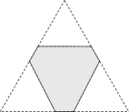
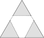
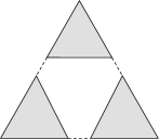
$\textstyle X(a_{-n})$	$\textstyle X^{c}(a_{-n})$	$\textstyle\overline{X^{c}(a_{-n})}$

Figure 7: An illustration of $\textstyle X(a_{-n})$, $\textstyle X^{c}(a_{-n})$, and $\textstyle\overline{X^{c}(a_{-n})}$ for the case with $\textstyle m=3$. The three sets are depicted as subsets (highlighted in gray and continuous lines) of the leader’s strategy space $\textstyle\Delta_{n}$. Dashed lines and circles indicate parts of $\textstyle\Delta_{n}$ which are not contained in the sets.

For every outcome configuration $\textstyle(S^{+},S^{-})$, we introduce the following sets:

$$\textstyle X(S^{+}):=\bigcap_{a_{-n}\in S^{+}}X(a_{-n})$$

and

$$\textstyle X(S^{-}):=\bigcap_{a_{-n}\in S^{-}}X^{c}(a_{-n}).$$

While the former is a closed polytope, the latter is the union of not open nor closed polytopes and, thus, it is not open nor closed itself. Similarly to $\textstyle X^{c}(a_{-n})$, $\textstyle X(S^{-})$ satisfies $\textstyle\operatorname*{bd}(X(S^{-}))\cap X(S^{-})\subseteq\operatorname*{bd}(\Delta_{n})$. The closure $\textstyle\overline{X(S^{-})}$ of $\textstyle X(S^{-})$ is obtained by taking the closure of each $\textstyle X^{c}(a_{-n})$. Hence, $\textstyle\overline{X(S^{-})}=\bigcap_{a_{-n}\in S^{-}}\overline{X^{c}(a_{-n})}$.

By leveraging these definitions, we can now focus on the set of all leader’s strategies which realize the outcome configuration $\textstyle(S^{+},S^{-})$, namely:

$$\textstyle X(S^{+})\cap X(S^{-}).$$

As for $\textstyle X(S^{-})$, $\textstyle X(S^{+})\cap X(S^{-})$ is not an open nor a closed set. Due to $\textstyle X(S^{+})$ being closed, the only points of $\textstyle\operatorname*{bd}(X(S^{+})\cap X(S^{-}))$ which are not in $\textstyle X(S^{+})\cap X(S^{-})$ itself are the very points in $\textstyle\operatorname*{bd}(X(S^{-}))$ which are not in $\textstyle X(S^{-})$. As a consequence, $\textstyle\overline{X(S^{+})\cap X(S^{-})}=X(S^{+})\cap\overline{X(S^{-})}$.

Let us define the set $\textstyle P:=\{(S^{+},S^{-}):S^{+}\in 2^{A_{F}}\wedge S^{-}=2^{A_{F}}\setminus S^{+}\}$, which contains all the outcome configurations of the game. The following theorem highlights the structure of $\textstyle f(x_{n})$, suggesting an iterative way of expressing the problem of computing $\textstyle\sup_{x_{n}\in\Delta_{n}}f(x_{n})$. We will rely on it when designing our algorithm.

Theorem 6.1

Let $\textstyle\displaystyle\psi(x_{n};S^{+}):=\min_{a_{-n}\in S^{+}}\sum_{a_{n}\in A_{n}}U^{a_{-n},a_{n}}x_{n}^{a_{n}}$. The following holds:

$$\sup_{x_{n}\in\Delta_{n}}f(x_{n})=\max_{\begin{subarray}{c}(S^{+},S^{-})\in P:\\ X(S^{+})\cap X(S^{-})\neq\emptyset\end{subarray}}\;\max_{x_{n}\in X(S^{+})\cap\overline{X(S^{-})}}\psi(x_{n};S^{+}).$$

Proof

Let $\textstyle\Delta^{\prime}_{n}$ be the set of leader’s strategies $\textstyle x_{n}$ for which there exists a pure NE in the followers’ game induced by $\textstyle x_{n}$, namely, $\textstyle\Delta^{\prime}_{n}:=\{x_{n}\in\Delta_{n}:f(x_{n})>-\infty\}$. Since, by definition, $\textstyle f(x_{n})=-\infty$ for any $\textstyle x_{n}\notin\Delta^{\prime}_{n}$ and the supremum of $\textstyle f(x_{n})$ is finite due to the finiteness of the payoffs (and assuming the followers’ game admits at least a pure NE for some $\textstyle x_{n}\in\Delta_{n}$), we can, w.l.o.g., focus on $\textstyle\Delta_{n}^{\prime}$ and solve $\textstyle\sup_{x_{n}\in\Delta_{n}^{\prime}}f(x_{n})$. In particular, the collection of the sets $\textstyle X(S^{+})\cap X(S^{-})\neq\emptyset$ which are obtained for all $\textstyle(S^{+},S^{-})\in P$ forms a partition of $\textstyle\Delta_{n}^{\prime}$. Due to the fact that, at any $\textstyle x_{n}\in X(S^{+})\cap X(S^{-})$, the only pure NEs induced by $\textstyle x_{n}$ in the followers’ game are those in $\textstyle S^{+}$, $\textstyle f(x_{n})=\psi(x_{n};S^{+})$. Since, as it is clear, the supremum of a function defined over a set is equal to the largest of the suprema of that function over the subsets of such set, we have:

$$\sup_{x_{n}\in\Delta_{n}}f(x_{n})=\max_{\begin{subarray}{c}(S^{+},S^{-})\in P:\\ X(S^{+})\cap X(S^{-})\neq\emptyset\end{subarray}}\sup_{x_{n}\in X(S^{+})\cap X(S^{-})}\psi(x_{n};S^{+}).$$

What remains to show is that, for all $\textstyle X(S^{+})\cap X(S^{-})\neq\emptyset$, the following relationship holds:

$$\textstyle\sup_{x_{n}\in X(S^{+})\cap X(S^{-})}\psi(x_{n};S^{+})=\max_{x_{n}\in X(S^{+})\cap\overline{X(S^{-})}}\psi(x_{n};S^{+}).$$

Since $\textstyle\psi(x_{n};S^{+})$ is a continuous function (it is the point-wise minimum of finitely many continuous functions), its supremum over $\textstyle X(S^{+})\cap X(S^{-})$ equals its maximum over the closure $\textstyle\overline{X(S^{+})\cap X(S^{-})}$ of that set. Hence, the relationship follows due to $\textstyle\overline{X(S^{+})\cap X(S^{-})}=X(S^{+})\cap\overline{X(S^{-})}$. ∎

In particular, Theorem 6.1 shows that $\textstyle f(x_{n})$ is a piecewise function with a piece for each set $\textstyle X(S^{+})\cap X(S^{-})$, each of which corresponding to the (continuous over its domain) piecewise-affine function $\textstyle\psi(x_{n};S^{+})$. It follows that the only discontinuities of $\textstyle f(x_{n})$, due to which $\textstyle f(x_{n})$ may admit a supremum but not a maximum, are those where, in $\textstyle\Delta_{n}$, $\textstyle x_{n}$ transitions from a set $\textstyle X(S^{+})\cap X(S^{-})$ to another one.

We show how to translate the formula in Theorem 6.1 into an algorithm by proving the following theorem:

Theorem 6.2

There exists a finite, exponential-time algorithm which computes $\textstyle\sup_{x_{n}\in\Delta_{n}}f(x_{n})$ and, whenever $\textstyle\sup_{x_{n}\in\Delta_{n}}f(x_{n})=\max_{x_{n}\in\Delta_{n}}f(x_{n})$, also returns a strategy $\textstyle x_{n}^{*}$ with $\textstyle f(x_{n}^{*})=\max_{x_{n}\in\Delta_{n}}f(x_{n})$.

Proof

The algorithm relies on the expression given in Theorem 6.1. All pairs $\textstyle(S^{+},S^{-})\in P$ can be constructed by enumeration in time exponential in the size of the instance. In particular, the set $\textstyle P$ contains $\textstyle 2^{m^{n-1}}$ outcome configurations, each corresponding to a bi-partition of the outcomes of the followers’ game into $\textstyle S^{+}$ and $\textstyle S^{-}$ (there are $\textstyle m^{n-1}$ such outcomes, due to having $\textstyle m$ actions and $\textstyle n-1$ followers).

Let us define, for every $\textstyle p\in F$, the following sets, parametric in $\textstyle\epsilon\geq 0$:

$$\textstyle\displaystyle D_{p}(a_{-n},a_{p}^{\prime};\epsilon):=\left\{\begin{array}[]{lr}x_{n}\in\Delta_{n}:&\displaystyle\sum_{a_{n}\in A_{n}}U_{p}^{a_{-n},a_{n}}x_{n}^{a_{n}}+\epsilon\leq\sum_{a_{n}\in A_{n}}U_{p}^{a_{-n}^{\prime},a_{n}}x_{n}^{a_{n}}\\ &\text{with }a_{-n}^{\prime}=(a_{1},\ldots,a_{p-1},a_{p}^{\prime},a_{p+1},\ldots,a_{n-1})\end{array}\right\},$$

$$\textstyle\displaystyle X^{c}(a_{-n};\epsilon):=\bigcup_{p\in F}\left(\bigcup_{a_{p}^{\prime}\in A_{p}\setminus\{a_{p}\}}D_{p}(a_{-n},a_{p}^{\prime};\epsilon)\right),$$

$$\textstyle X(S^{-};\epsilon):=\bigcap_{a_{-n}\in S^{-}}X^{c}(a_{-n};\epsilon).$$

Notice that, when $\textstyle\epsilon=0$, we have $\textstyle D_{p}(a_{-n},a_{p}^{\prime};0)=\overline{D_{p}(a_{-n},a_{p}^{\prime})}$ and $\textstyle X(S^{-};0)=\overline{X(S^{-})}$. Hence, we can verify whether $\textstyle X(S^{+})\cap X(S^{-})\neq\emptyset$ by verifying whether there exists some $\textstyle\epsilon>0$ such that $\textstyle X(S^{+})\cap X(S^{-};\epsilon)\neq\emptyset$. This can be done by solving the following problem and checking the strict positivity of $\textstyle\epsilon$ in its solution:

$$\begin{array}[]{ll}\displaystyle\max_{\epsilon,x_{n}}&\epsilon\\ \text{s.t.}&x_{n}\in X(S^{+})\cap X(S^{-};\epsilon)\\ &\epsilon\geq 0\\ &x_{n}\in\Delta_{n}.\end{array}$$ (8)

Problem (8) can be cast as an MILP. To see this, observe that each $\textstyle X^{c}(a_{-n};\epsilon)$ can be expressed as an MILP with a binary variable for each term of the disjunction which composes it, namely:

$$\textstyle\displaystyle\sum_{a_{n}\in A_{n}}U_{p}^{a_{-n},a_{n}}x_{n}^{a_{n}}+\epsilon\leq\sum_{a_{n}\in A_{n}}U_{p}^{a_{-n}^{\prime},a_{n}}x_{n}^{a_{n}}+M_{p}^{a_{-n},a_{p}^{\prime}}z_{p}^{a_{-n},a_{p}^{\prime}}$$

$$\textstyle\displaystyle\hskip 14.22636pt\forall p\in F,a_{p}^{\prime}\in A_{p}\setminus\{a_{p}\},\text{with }a_{-n}^{\prime}=(a_{1},\ldots,a_{p-1},a_{p}^{\prime},a_{p+1},\ldots,a_{n-1})$$ (9a)

$$\textstyle\displaystyle\sum_{p\in F}\sum_{a_{p}^{\prime}\in A_{p}\setminus\{a_{p}\}}(1-z_{p}^{a_{-n},a_{p}^{\prime}})=1$$ (9b)

$$\textstyle\displaystyle z_{p}^{a_{-n},a_{p}^{\prime}}\in\{0,1\} \textstyle\displaystyle\forall p\in F,a_{p}^{\prime}\in A_{p}\setminus\{a_{p}\}$$ (9c)

$$\textstyle\displaystyle x_{n}\in\Delta_{n}$$ (9d)

$$\textstyle\displaystyle\epsilon\geq 0.$$ (9e)

In Constraints (9), the constant $\textstyle M_{p}^{a_{-n},a_{p}^{\prime}}$, which satisfies $\textstyle M_{p}^{a_{-n},a_{p}^{\prime}}=\max_{a_{n}\in A_{n}}\{U_{p}^{a_{-n},a_{n}}-U_{p}^{a_{-n}^{\prime},a_{n}}\}$, is key to deactivate any instance of Constraints (9a) when the corresponding $\textstyle z_{p}^{a_{-n},a_{p}^{\prime}}$ is equal to 1. The set $\textstyle X(S^{-};\epsilon)$ is obtained by simultaneously imposing Constraints (9) for all $\textstyle a_{-n}\in S^{-}$.

After verifying $\textstyle X(S^{+})\cap\overline{X(S^{-})}\neq\emptyset$ by solving Problem (8), the value of $\textstyle\max_{x_{n}\in X(S^{+})\cap\overline{X(S^{-})}}\psi(x_{n};S^{+})$ can be computed in, at most, exponential time by solving the following MILP:

$$\begin{array}[]{lll}\max_{\eta,x_{n}}&\eta\\ \text{s.t.}&\eta\leq\displaystyle\sum_{a_{n}\in A_{n}}U_{n}^{a_{-n},a_{n}}x_{n}^{a_{n}}&\forall a_{-n}\in S^{+}\\ &x_{n}\in X(S^{+})\cap X(S^{-};0)\\ &\eta\in\mathbb{R}\\ &x_{n}\in\Delta_{n},\end{array}$$ (10)

where the first constraint accounts for the maxmin aspect of the problem. The largest value of $\textstyle\eta$ found over all sets $\textstyle X(S^{+})\cap X(S^{-})$, for all $\textstyle(S^{+},S^{-})\in P$, corresponds to $\textstyle\sup_{x_{n}\in\Delta_{n}}f(x_{n})$.

To verify whether $\textstyle f(x_{n})$ admits $\textstyle\max_{x_{n}\in\Delta_{n}}f(x_{n})$ and, if it does, compute it, we solve, in the algorithm, the following problem (rather than the aforementioned $\textstyle\max_{x_{n}\in X(S^{+})\cap\overline{X(S^{-})}}\psi(x_{n};S^{+})$):

$$\operatorname*{lex--max}_{\epsilon\geq 0,x_{n}\in X(S^{+})\cap X(S^{-};\epsilon)}[\psi(x_{n};S^{+});\epsilon].$$ (11)

This problem calls for a pair $\textstyle(x_{n},\epsilon)$ with $\textstyle x_{n}\in X(S^{+})\cap X(S^{-};\epsilon)$ such that, among all pairs which maximise $\textstyle\psi(x_{n};S^{+})$, $\textstyle\epsilon$ is as large as possible. This way, in any solution $\textstyle(x_{n},\epsilon)$ with $\textstyle\epsilon>0$ we have $\textstyle x_{n}\in X(S^{+})\cap X(S^{-})$ (rather than $\textstyle x_{n}\in X(S^{+})\cap\overline{X(S^{-})}$). Since, there, $\textstyle\psi(x_{n};S^{+})=f(x_{n})$, we conclude that $\textstyle f(x_{n})$ admits a maximum (equal to the value of the supremum) if $\textstyle\epsilon>0$, whereas it only admits a supremum if $\textstyle\epsilon=0$.

Problem (11) can be solved in, at most, exponential time by solving the following lex-MILP:

$$\begin{array}[]{lll}\max_{\eta,x_{n},\epsilon}&\left[\eta\ ;\epsilon\right]\\ \text{s.t.}&\eta\leq\displaystyle\sum_{a_{n}\in A_{n}}U_{n}^{a_{-n},a_{n}}x_{n}^{a_{n}}&\forall a_{-n}\in S^{+}\\ &x_{n}\in X(S^{+})\cap X(S^{-};\epsilon)\\ &\eta\in\mathbb{R}\\ &\epsilon\geq 0\\ &x_{n}\in\Delta_{n},\end{array}$$ (12)

where $\textstyle\eta$ is maximised first, and $\textstyle\epsilon$ second. In practice, it suffices to solve two MILPs in sequence: one in which the first objective function is maximised, and then another one in which the second objective function is maximised after imposing the first objective function to be equal to its optimal value. ∎

6.1.2 Finding an $\textstyle\alpha$-Approximate Strategy

For those cases where $\textstyle f(x_{n})$ does not admit a maximum, we look for a strategy $\textstyle\hat{x}_{n}$ such that, for a given $\textstyle\alpha>0$, $\textstyle\sup_{x_{n}\in\Delta_{n}}f(x_{n})-f(\hat{x}_{n})\leq\alpha$, i.e., for an (additively) $\textstyle\alpha$-approximate strategy $\textstyle\hat{x}_{n}$. Its existence is guaranteed by the following lemma.

Lemma 3

Consider the sets $\textstyle X\subseteq\mathbb{R}^{n}$, for some $\textstyle n\in\mathbb{N}$, and $\textstyle Y\subseteq\mathbb{R}$, and a function $\textstyle f:X\rightarrow Y$ with $\textstyle s:=\sup_{x\in X}f(x)$, satisfying $\textstyle s<\infty$. Then, for any $\textstyle\alpha\in(0,s]$, there exists an $\textstyle x\in X:s-f(x)\leq\alpha$.

Proof

By negating the conclusion, we deduce the existence of some $\textstyle\alpha\in(0,s]$ such that, for every $\textstyle x\in X$, $\textstyle s-f(x)>\alpha$. But, then, for all $\textstyle x\in X$, we have $\textstyle f(x)<s-\alpha$, which implies $\textstyle s=\sup_{x\in X}f(x)\leq s-\alpha<s$: a contradiction. ∎

After running the algorithm we outlined in the proof of Theorem 6.1 to compute the value of the supremum, an $\textstyle\alpha$-approximate strategy $\textstyle\hat{x}_{n}$ can be computed, a posteriori, thanks to the following result:

Theorem 6.3

Assume that $\textstyle f(x_{n})$ does not admit a maximum over $\textstyle\Delta_{n}$ and that, according to the formula in Theorem 6.1, $\textstyle s:=\sup_{x_{n}\in\Delta_{n}}f(x_{n})$ is attained at some outcome configuration $\textstyle(S^{+},S^{-})$. Then, an $\textstyle\alpha$-approximate strategy $\textstyle\hat{x}_{n}$ can be computed for any $\textstyle\alpha>0$ in, at most, exponential time by solving the following MILP:

$$\begin{array}[]{llr}\max_{\begin{subarray}{c}\epsilon,x_{n}\end{subarray}}&\epsilon\\ \text{{\em s.t.}}&\displaystyle\sum_{a_{n}\in A_{n}}U_{n}^{a_{-n},a_{n}}x_{n}^{a_{n}}\geq s-\alpha&\quad\forall a_{-n}\in S^{+}\\ &x_{n}\in X(S^{+})\cap X(S^{-};\epsilon)\\ &\epsilon\geq 0\\ &x_{n}\in\Delta_{n}.\end{array}$$ (13)

Proof

Let $\textstyle x_{n}^{*}\in X(S^{+}\cap S^{-})$ be the strategy where the supremum is attained according to the formula in Theorem 6.1, namely, where $\textstyle\psi(x_{n}^{*},S^{+})=\max_{\begin{subarray}{c}x_{n}\in X(S^{+})\cap\overline{X(S^{-})}\end{subarray}}\psi(x_{n};S^{+})=s$. Problem (13) calls for a solution $\textstyle x_{n}$ of value at least $\textstyle s-\alpha$ (thus, for an $\textstyle\alpha$-approximate strategy) belonging to $\textstyle X(S^{+})\cap X(S^{-};\epsilon)$ with $\textstyle\epsilon$ as large as possible, whose existence is guaranteed by Lemma 3. Let $\textstyle(\hat{x}_{n},\hat{\epsilon})$ be an optimal solution to Problem (13). If $\textstyle\hat{\epsilon}>0$, $\textstyle\hat{x}_{n}\in X(S^{+})\cap X(S^{-})$ (rather than $\textstyle\hat{x}_{n}\in X(S^{+})\cap\overline{X(S^{-})}$). Thus, $\textstyle f(x_{n})$ is continuous at $\textstyle x_{n}=\hat{x}_{n}$, implying $\textstyle\psi(x_{n};S^{+})=f(x_{n})$. Therefore, by playing $\textstyle\hat{x}_{n}$, the leader achieves a utility of, at least, $\textstyle s-\alpha$. ∎

6.1.3 Outline of the Explicit Enumeration Algorithm

The complete enumerative algorithm is detailed in Algorithm 1. In the pseudocode, CheckEmptyness$\textstyle(S^{+},S^{-})$ is a subroutine which looks for a value of $\textstyle\epsilon\geq 0$ which is optimal for Problem (8), while Solve-lex-MILP$\textstyle(S^{+},S^{-})$ is another subroutine which solves Problem (12). Due to the lexicographic nature of the algorithm, $\textstyle f(x_{n})$ admits a maximum if and only the algorithm returns a solution with $\textstyle best.\epsilon^{*}>0$, whereas, if $\textstyle best.\epsilon^{*}=0$, $\textstyle x_{n}^{*}$ is just a strategy where $\textstyle\sup_{x_{n}\in\Delta_{n}}f(x_{n})$ is attained (in the sense of Theorem 6.1). In the latter case, an $\textstyle\alpha$-approximate strategy is found by invoking the procedure Solve-MILP-approx$\textstyle(best.S^{+},best.S^{-},best\_value)$, which solves Problem (13) on the outcome configuration $\textstyle(best.S^{+},best.S^{-})$ on which the supremum has been found.

Algorithm 1 Explicit Enumeration

1:function Explicit Enumeration

2:     $\textstyle best\leftarrow nil$

3:     $\textstyle best\_val\leftarrow-\infty$

4:     for all $\textstyle S^{+}\in A_{F}$ do

5:         $\textstyle S^{-}\leftarrow A_{F}\setminus S^{+}$

6:         $\textstyle(\epsilon,\cdot)\leftarrow\textsf{CheckEmptyness}(S^{+},S^{-})$ $\textstyle\triangleright$ Solve MILP Problem (8)

7:         if $\textstyle\epsilon>0$ then

8:              $\textstyle(\eta,\epsilon^{*},x_{n}^{*})\leftarrow\textsf{Solve-lex-MILP}(S^{+},S^{-})$ $\textstyle\triangleright$ Solve lex-MILP Problem (12)

9:              if $\textstyle\eta>best\_val$ then

10:                  $\textstyle best\leftarrow(S^{+},S^{-},x_{n}^{*},\epsilon^{*})$

11:                  $\textstyle best\_val\leftarrow\eta$

12:              end if

13:         end if

14:     end for

15:     if $\textstyle best.\epsilon^{*}=0$ then

16:         $\textstyle\hat{x}_{n}\leftarrow best.x_{n}$

17:     else

18:         $\textstyle\hat{x}_{n}\leftarrow\textsf{Solve-MILP-approx}(best.S^{+},best.S^{-},best\_val)$ $\textstyle\triangleright$ Solve MILP Problem (13)

19:     end if

20:     return $\textstyle best\_val$, $\textstyle best.x_{n}^{*}$, $\textstyle\hat{x}_{n}$

21:end function

6.2 Branch-and-Bound Algorithm

As it is clear, computing $\textstyle\sup_{x_{n}\in\Delta_{n}}f(x_{n})$ with the enumerative algorithm can be impractical for any game of interesting size, as it requires the explicit enumeration of all the outcome configurations of a game—many of which will, incidentally, yield empty regions $\textstyle X(S^{+})\cap X(S^{-})$. A more efficient algorithm, albeit one still running in exponential time in the worst-case, can be designed by relying on a branch-and-bound scheme.

6.2.1 Computing $\textstyle\sup_{x_{n}\in\Delta_{n}}f(x_{n})$

Rather than defining $\textstyle S^{-}=A_{F}\setminus S^{+}$, assume now $\textstyle S^{-}\subseteq A_{F}\setminus S^{+}$. In this case, we call the corresponding pair $\textstyle(S^{+},S^{-})$ a relaxed outcome configuration.

Starting from any followers’ action profile $\textstyle a_{-n}\in A_{F}$ with $\textstyle X(a_{-n})\neq\emptyset$, the algorithm constructs and explores, through a sequence of branching operations, two search trees, whose nodes correspond to relaxed outcome configurations. One tree accounts for the case where $\textstyle a_{-n}$ is an NE and contains the relaxed outcome configuration $\textstyle(S^{+},S^{-})=(\{a_{-n}\},\emptyset)$ as root node. The other tree accounts for the case where $\textstyle a_{-n}$ is not an NE, featuring as root node the relaxed outcome configuration $\textstyle(S^{+},S^{-})=(\emptyset,\{a_{-n}\})$.

If $\textstyle S^{-}\subset A_{F}\setminus S^{+}$ (which can often be the case when relaxed outcome configurations are adopted), solving $\textstyle\max_{x_{n}\in X(S^{+})\cap\overline{X(S^{-})}}\psi(x_{n};S^{+})$ might not give a strategy $\textstyle x_{n}$ for which the only pure NEs in the followers’ game it induces are those in $\textstyle S^{+}$, even if $\textstyle x_{n}\in X(S^{+})\cap X(S^{-})$ (rather than $\textstyle x_{n}\in X(S^{+})\cap\overline{X(S^{-})}$). This is because, due to $\textstyle S^{+}\cup S^{-}\subset A_{F}$, there might be another action profile, say $\textstyle a_{-n}^{\prime}\in A_{F}\setminus(S^{+}\cup S^{-})$, providing the leader with a utility strictly smaller than that corresponding to all the action profiles in $\textstyle S^{+}$. Since, if this is the case, the followers would respond to $\textstyle x_{n}$ by playing $\textstyle a_{-n}^{\prime}$ rather than any of the action profiles in $\textstyle S^{+}$, $\textstyle\max_{x_{n}\in X(S^{+})\cap\overline{X(S^{-})}}\psi(x_{n};S^{+})$ could be, in general, strictly larger than $\textstyle\sup_{x_{n}\in\Delta_{n}}f(x_{n})$, thus not being a valid candidate for the computation of the latter.

In order to detect whether one such $\textstyle a_{-n}^{\prime}$ exists, it suffices to carry out a feasibility check (on $\textstyle x_{n}$) by looking for, in the followers’ game, a pure NE different from those in $\textstyle S^{-}$ (which may become NEs on $\textstyle\operatorname*{bd}(X(S^{+})\cap X(S^{-})$) which minimises the leader’s utility—this can be done by inspection in $\textstyle O(m^{n-1})$. If the feasibility check returns some $\textstyle a_{-n}^{\prime}\notin S^{+}$, the branch-and-bound tree is expanded by performing a branching operation. Two nodes are introduced: a left node with $\textstyle(S_{L}^{+},S_{L}^{-})$ where $\textstyle S_{L}^{+}=S^{+}\cup\{a_{-n}^{\prime}\}$ and $\textstyle S_{L}^{-}=S^{-}$ (which accounts for the case where $\textstyle a_{-n}^{\prime}$ is a pure NE), and a right node with $\textstyle(S_{R}^{+},S_{R}^{-})$ where $\textstyle S_{R}^{+}=S^{+}$ and $\textstyle S_{R}^{-}=S^{-}\cup\{a_{-n}^{\prime}\}$ (which accounts for the case where $\textstyle a_{-n}^{\prime}$ is not a pure NE). If, differently, $\textstyle a_{-n}^{\prime}\in S^{+}$, then $\textstyle\psi(x_{n};S^{+})$ represents a valid candidate for the computation of $\textstyle\sup_{x_{n}\in\Delta_{n}}f(x_{n})$ and, thus, no further branching is needed (and $\textstyle(S^{+},S^{-})$ is a leaf node).

The bounding aspect of the algorithm is a consequence of the following proposition:

Proposition 8

Solving $\textstyle\max_{x_{n}\in X(S^{+})\cap\overline{X(S^{-})}}\psi(x_{n};S^{+})$ for some relaxed outcome configuration $\textstyle(S^{+},S^{-})$ gives an upper bound on the leader’s utility under the assumption that all followers’ action profiles in $\textstyle S^{+}$ constitute an NE and those in $\textstyle S^{-}$ do not.

Proof

Due to $\textstyle(S^{+},S^{-})$ being a relaxed outcome configuration, there could be outcomes not in $\textstyle S^{+}$ which are NEs for some $\textstyle x_{n}\in X(S^{+})\cap\overline{X(S^{-})}$. Due to $\textstyle\psi(x_{n};S^{+})$ being defined as $\textstyle\min_{a_{-n}\in S^{+}}\sum_{a_{n}\in A_{n}}U^{a_{-n},a_{n}}x_{n}^{a_{n}}$, ignoring any such NE at any $\textstyle x_{n}\in X(S^{+})\cap\overline{X(S^{-})}$ can only result in the $\textstyle\min$ operator running on fewer outcomes $\textstyle a_{-n}$, thus overestimating $\textstyle\psi(x_{n};S^{+})$ and, ultimately, $\textstyle f(x_{n})$. The claim, thus, follows. ∎

As a consequence of Proposition 8, optimal values obtained when computing the value of $\textstyle\max_{x_{n}\in X(S^{+})\cap\overline{X(S^{-})}}\psi(x_{n};S^{+})$ throughout the search tree can be used as bounds as in a standard branch-and-bound method.

Since $\textstyle\max_{x_{n}\in X(S^{+})\cap\overline{X(S^{-})}}\psi(x_{n};S^{+})$ is not well-defined for nodes where $\textstyle S^{+}=\emptyset$, for them we solve, rather than an instance of Problem (12), a restriction of the optimistic problem (see Section 3) with constraints imposing that all followers’ action profiles in $\textstyle S^{-}$ are not NEs. We employ the following formulation, which we introduce directly for the lexicographic case:

$$\textstyle\displaystyle\max_{y,x_{n},\epsilon} \textstyle\displaystyle\;\left[\sum_{a\in A}U_{n}^{a_{-n},a_{n}}y^{a_{-n}}x_{n}^{a_{n}};\epsilon\right]$$ (14a)

s.t. $$\textstyle\displaystyle\sum_{a_{-n}\in A_{F}}y^{a_{-n}}=1$$ (14b)

$$\textstyle\displaystyle y^{a_{-n}}\sum_{a_{n}\in A_{n}}(U_{p}^{a_{-n},a_{n}}-U_{p}^{a_{-n}^{\prime},a_{n}})x_{n}^{a_{n}}\geq 0 \textstyle\displaystyle\forall p\in F,a_{-n}\in A_{F},a_{p}^{\prime}\in A_{p}\setminus\{a_{p}\}$$

$$\textstyle\displaystyle\text{with }a_{-n}^{\prime}=a_{1},\dots,a_{p-1},a_{p}^{\prime},a_{p+1},\dots,a_{n-1}$$ (14c)

$$\textstyle\displaystyle y^{a_{-n}}\in\{0,1\} \textstyle\displaystyle\forall a_{-n}\in A_{F}$$ (14d)

$$\textstyle\displaystyle x_{n}\in\Delta_{n}$$ (14e)

$$\textstyle\displaystyle x_{n}\in X(S^{-};\epsilon).$$ (14f)

The problem can be turned into a lex-MILP by linearizing each bilinear product $\textstyle y^{a_{-n}}x_{n}^{a_{n}}$ by means of McCormick’s envelope and by restating Constraint (14f) as done in the MILP Constraints (9).

6.2.2 Finding an $\textstyle\alpha$-Approximate Strategy

Notice that, in the context of the branch-and-bound algorithm, an $\textstyle\alpha$-approximate strategy $\textstyle\hat{x}_{n}$ cannot be found by just relying on the a posteriori procedure outlined in Theorem 6.3. This is because, when $\textstyle(S^{+},S^{-})$ is a relaxed outcome configuration, there might be an action profile $\textstyle a_{-n}^{\prime}\in A_{F}\setminus(S^{+}\cup S^{-})$ (i.e., one not accounted for in the relaxed outcome configuration) which not only is a NE in the followers’ game induced by $\textstyle\hat{x}_{n}$, but which also provides the leader with a utility strictly smaller than $\textstyle\psi(\hat{x}_{n};S^{+})$. If this is the case, the strategy $\textstyle\hat{x}_{n}$ found with the procedure of Theorem 6.3 may return a utility arbitrarily smaller than the supremum $\textstyle s$ and, in particular, smaller than $\textstyle s-\alpha$.

To cope with this shortcoming and establish whether such an $\textstyle a_{-n}^{\prime}$ exists, we first compute $\textstyle\hat{x}_{n}$ according to the a posteriori procedure of Theorem 6.3 and, then, perform a feasibility check. If we obtain an action profile $\textstyle a_{-n}^{\prime}\in S^{+}$, $\textstyle\hat{x}_{n}$ is then an $\textstyle\alpha$-approximate strategy and the algorithm halts. If, differently, we obtain some $\textstyle a_{-n}^{\prime}\notin S^{+}$ for which the leader obtains a utility strictly smaller than $\textstyle\psi(\hat{x}_{n};S^{+})$, we carry out a branching operation, creating a left and a right child node in which $\textstyle a_{-n}^{\prime}$ is added to, respectively, $\textstyle S^{+}$ or $\textstyle S^{-}$. This procedure is then applied on both nodes, recursively, until a strategy $\textstyle\hat{x}_{n}$ for which the feasibility check returns an action profile in $\textstyle S^{+}$ is found. Such a strategy is, by construction, $\textstyle\alpha$-approximate.

Observe that, due to the correctness of the algorithm for the computation of the supremum, there cannot be at $\textstyle x_{n}^{*}$ an NE $\textstyle a_{-n}^{\prime}$ worse than the worst-case one in $\textstyle S^{+}$. If a new outcome $\textstyle a_{-n}^{\prime}$ becomes the worst-case NE at $\textstyle\hat{x}_{n}$, due to the fact that it is not a worst-case NE at $\textstyle x_{n}^{*}$, there must be a strategy $\textstyle\tilde{x}_{n}$ which is a convex combination of $\textstyle x_{n}^{*}$ and $\textstyle\hat{x}_{n}$ where either $\textstyle a_{-n}^{\prime}$ is not an NE or, if it is, it yields a leader’s utility not worse than that obtained with the worst-case NE in $\textstyle S^{+}$. An $\textstyle\alpha$-approximate strategy is thus guaranteed to be found on the segment joining $\textstyle\tilde{x}_{n}$ and $\textstyle x_{n}^{*}$ by applying Lemma 3 with $\textstyle X$ equal to that segment. Thus, the algorithm is guaranteed to converge.

6.2.3 Outline of the Branch-and-Bound Algorithm

The complete outline of the branch-and-bound algorithm is detailed in Algorithm 2. $\textstyle\mathcal{F}$ is the frontier of the two search trees, containing all nodes which have yet to be explored. Initialize$\textstyle()$ is a subprocedure which creates the root nodes of the two search trees, while pick$\textstyle()$ extracts from $\textstyle\mathcal{F}$ the next node to be explored. FeasibilityCheck$\textstyle(x_{n},S^{-})$ performs the feasibility check operation for the leader’s strategy $\textstyle x_{n}$, looking for the worst-case pure NE in the game induced by $\textstyle x_{n}$ and ignoring any outcome in $\textstyle S^{-}$. CreateNode$\textstyle(S^{+},S^{-})$ (detailed in Algorithm 3) adds a new node to $\textstyle\mathcal{F}$, also computing its upper bound and the corresponding values of $\textstyle x_{n}$ and $\textstyle\epsilon$. More specifically, CreateNode$\textstyle(S^{+},S^{-})$ performs the same operations of a generic step of the enumerative procedure in Algorithm 1 for a given $\textstyle S^{+}$ and $\textstyle S^{-}$, with the only difference that, here, we invoke the subprocedure Solve-lex-MILP-Opt$\textstyle(S^{+},S^{-})$ whenever $\textstyle S^{+}=\emptyset$, by which Problem (14) is solved, while we invoke Solve-lex-MILP$\textstyle(S^{+},S^{-})$, which solves Problem (12), if $\textstyle S^{+}\neq\emptyset$. In the last part of the algorithm, $\textstyle\textsf{Solve-MILP-approx}(best.S^{+},best.S^{-},best\_val)$ attempts to compute an $\textstyle\alpha$-approximate strategy as done in Algorithm 1. In case the feasibility check fails for it, we resort to calling the procedure $\textstyle\textsf{Branch-and-Bound-approx}(best.S^{+},best.S^{-},best.x_{n}^{*})$ which runs a second branch-and-bound method, as described in Subsection 6.2.2, until an $\textstyle\alpha$-approximate solution is found.

Algorithm 2 Branch-and-Bound

1:function Branch-and-Bound

2:     $\textstyle best\leftarrow nil,\quad lb\leftarrow-\infty,\quad ub\leftarrow\infty$

3:     $\textstyle\mathcal{F}\leftarrow\textsf{Initialize()}$

4:     while $\textstyle\mathcal{F}\neq\emptyset$ do

5:         $\textstyle node\leftarrow\mathcal{F}.\textsf{pick}()$

6:         if $\textstyle node.ub>lb$ then

7:              $\textstyle a_{-n}\leftarrow\textsf{FeasibilityCheck}(node.x_{n}^{*},node.S^{-})$

8:              if $\textstyle a_{-n}\in node.S^{+}$ then

9:                  $\textstyle best\leftarrow(node.S^{+},node.S^{-},node.x_{n}^{*},node.\epsilon^{*})$

10:                  $\textstyle lb\leftarrow node.ub$

11:              else

12:                  $\textstyle S^{+}_{L}=node.S^{+}\cup\{a_{-n}\}$

13:                  $\textstyle\mathcal{F}\leftarrow\mathcal{F}+\textsf{CreateNode}(S^{+}_{L},node.S^{-})$

14:                  $\textstyle S^{-}_{R}=node.S^{-}\cup\{a_{-n}\}$

15:                  $\textstyle\mathcal{F}\leftarrow\mathcal{F}+\textsf{CreateNode}(node.S^{+},S^{-}_{R})$

16:              end if

17:              $\textstyle\displaystyle ub\leftarrow\max_{node\in\mathcal{F}}\left\{node.ub\right\}$

18:         end if

19:     end while

20:     if $\textstyle best.\epsilon^{*}=0$ then

21:         $\textstyle\hat{x}_{n}\leftarrow best.x_{n}^{*}$

22:     else

23:         $\textstyle\hat{x}_{n}\leftarrow\textsf{Solve-MILP-approx}(best.S^{+},best.S^{-},best\_val)$ $\textstyle\triangleright$ Solve MILP Problem (13)

24:         $\textstyle a_{-n}^{\prime}\leftarrow\textsf{FeasibilityCheck}(\hat{x}_{n},best.S^{-})$

25:         if $\textstyle a_{-n}^{\prime}\notin best.S^{+}$ then

26:              $\textstyle\hat{x}_{n}\leftarrow\textsf{Branch-and-Bound-approx}(best.S^{+},best.S^{-},best.x_{n}^{*})$

27:         end if

28:     end if

29:     return $\textstyle ub$, $\textstyle best.x_{n}^{*},\hat{x}_{n}$

30:end function

Algorithm 3 CreateNode

1:function CreateNode($\textstyle S^{+},S^{-}$)

2:     $\textstyle(\epsilon,\cdot)\leftarrow\textsf{CheckEmptyness}(S^{+},S^{-})$ $\textstyle\triangleright$ Solve MILP Problem (8)

3:     if $\textstyle\epsilon>0$ then

4:         $\textstyle node\leftarrow\textsf{EmptyNode}()$

5:         $\textstyle node.S^{+}\leftarrow S^{+}$

6:         $\textstyle node.S^{-}\leftarrow S^{-}$

7:         if $\textstyle S^{+}=\emptyset$ then

8:              $\textstyle(\eta,\epsilon^{*},x_{n}^{*})\leftarrow\textsf{Solve-lex-MILP-Opt}(S^{+},S^{-})$ $\textstyle\triangleright$ Solve lex-MILP Problem (14)

9:         else

10:              $\textstyle(\eta,\epsilon^{*},x_{n}^{*})\leftarrow\textsf{Solve-lex-MILP}(S^{+},S^{-})$ $\textstyle\triangleright$ Solve lex-MILP Problem (12)

11:         end if

12:         $\textstyle node.ub\leftarrow\eta$

13:         $\textstyle node.x_{n}^{*}\leftarrow x_{n}^{*}$

14:         $\textstyle node.\epsilon^{*}\leftarrow\epsilon^{*}$

15:         return $\textstyle node$

16:     end if

17:     return $\textstyle\emptyset$

18:end function

7 Experimental Evaluation

We carry out, in this section, an experimental evaluation of the equilibrium-finding algorithms introduced in the previous sections. In particular, we compare three methods:

• QCQP: the QCQP Formulation (5), which we solve with the state-of-the-art spatial-branch-and-bound code BARON Sahinidis (2014); note that, as indicated in Sahinidis (2014), global optimality cannot be guaranteed by BARON if the feasible region of the problem at hand is not bounded, which is the case of Formulation (5). Hence, solutions obtained with QCQP are, in the general case, feasible but not necessarily optimal.

• MILP: the MILP Formulation (7), with dual variables artificially bounded by $\textstyle M$, which we solve with the state-of-the-art MILP solver Gurobi $\textstyle 7.0.2$; experiments with different values of $\textstyle M$ are reported.

• BnB-sup: the ad hoc branch-and-bound algorithm we proposed, described in Subsection 6.2 and better detailed in Algorithm 2, which we run to compute $\textstyle\sup_{x_{n}\in\Delta_{n}}f(x_{n})$, i.e., the supremum of the leader’s utility. The algorithm is coded in Python $\textstyle 2.7$. The different MILP subproblems that are encountered during its execution are solved with Gurobi 7.0.2.

• BnB-$\textstyle\alpha$: the ad hoc branch-and-bound algorithm we proposed, run to find, if there is no $\textstyle x_{n}\in\Delta_{n}$ at which the value of the supremum is attained, an $\textstyle\alpha$-approximate strategy. Results obtained with different values of $\textstyle\alpha$ are illustrated.

We conduct our experiments on a testbed of normal-form game instances built with GAMUT, a widely adopted suite of game instance generators Nudelman et al (2004). All the game instances we used are of RandomGame class, with their payoffs independently drawn from a uniform distribution with values in the range $\textstyle[1,100]$. The testbed contains games with $\textstyle n=3,4,5$ players (i.e., with $\textstyle 2,3,4$ followers). We generate instances with $\textstyle m\in\{4,6,\ldots,20,25,\ldots,70\}$ actions when $\textstyle n=3$, and $\textstyle m\in\{3,4,\ldots,15\}$ actions when $\textstyle n=4,5$. In order to obtain statistically more robust results, the testbed includes $\textstyle 30$ different instances for each pair of $\textstyle n$ and $\textstyle m$.

Throughout the experiments and for each algorithm, we collect the following figures for each game, which we then average over all the 30 game instances in the testbed with the same values of $\textstyle n$ and $\textstyle m$:

• Time: computing time, in seconds and up to the time limit, needed to solve the game (i.e., to compute an equilibrium).

• LB: the lower-bound corresponding to the value of the best feasible solution the algorithm managed to find before halting either due to convergence or due to an elapsed time limit; by playing the strategy $\textstyle x_{n}$ encoded in this solution, the leader is guaranteed to obtain a utility equal to at least LB; in the average, this value is only considered for instances where a feasible solution is found.

• Gap: the additive gap of the returned solution, measured as UB - LB, where UB is the upper-bound returned by the algorithm on the value of an optimal solution to the equilibrium-finding search problem. Note that, when solving the two restricted formulations, i.e., the QCQP Formulation (5) and the MILP Formulation (7), Gap corresponds to the gap “internal” to the solution method, thus being, in general, not valid for the original, unrestricted problem. This is not the case for BnB-sup and BnB-$\textstyle\alpha$, for which Gap is a correct additive estimate of the difference between the best found LB and the value of the supremum (overestimated by UB).

We also report, for each value of $\textstyle n$ and $\textstyle m$, the following two figures:

• Opt: the percentage of instances solved to optimality. The figure is only reported for BnB since, as previously explained, optimality cannot be guaranteed for the solutions to the two formulations.

• Feas: the percentage of instances for which a feasible solution has been found. We report the figure for the two mathematical programming formulations as an alternative to Opt.

The experiments are run on a UNIX machine with a total of 32 cores working at 2.3 GHz, equipped with 128 GB of RAM. All the computations are carried out on a single thread, with a time limit of 3600 seconds per instance.

7.1 Experimental Results with Two Followers

We report, first, the results obtained on games with two followers (i.e., with $\textstyle n=3$), which are summarized in Table 2. In particular, the table compares:

• QCQP;

• MILP with three values of $\textstyle M$, namely, $\textstyle M=10,100,1000$;

• BnB-sup;

• BnB-$\textstyle\alpha$, with three values of $\textstyle\alpha$, namely, $\textstyle\alpha=0.1,1,10$.

					MILP				MILP				MILP								BnB-$\textstyle\alpha$		BnB-$\textstyle\alpha$		BnB-$\textstyle\alpha$
	QCQP				$\textstyle M=10$				$\textstyle M=100$				$\textstyle M=1000$				BnB-sup				$\textstyle\alpha=0.1$		$\textstyle\alpha=1$		$\textstyle\alpha=10$
$\textstyle m$	Time	LB	Gap	Fea	Time	LB	Gap	Fea	Time	LB	Gap	Fea	Time	LB	Gap	Fea	Time	LB	Gap	Opt	Time		Time		Time
4	3600	81.3	18.7	100	2	83.5	0.0	100	1	85.8	0.0	100	1	85.3	0.0	100	1	85.7	0.0	100	1		1		0
6	3600	80.4	19.6	100	761	90.2	0.1	100	137	91.7	0.0	100	173	91.8	0.0	100	2	91.9	0.0	100	3		2		2
8	3600	70.6	29.4	100	1788	92.9	1.1	100	1419	93.8	0.9	100	1760	93.9	1.1	100	5	94.5	0.0	100	9		9		9
10	3600	67.2	32.8	100	2672	90.3	6.7	97	2161	95.4	1.7	100	2116	95.2	1.9	100	7	96.7	0.0	100	17		16		17
12	3600	63.3	36.7	100	3456	84.1	13.0	100	3184	89.6	7.7	100	3117	86.7	10.4	100	15	96.8	0.0	100	39		39		32
14	3600	57.3	42.7	97	3600	64.1	35.9	80	3585	68.3	30.9	100	3591	66.0	33.1	100	20	97.9	0.0	100	72		79		78
16	3600	45.2	54.8	77	3600	34.1	65.9	50	3600	61.7	38.3	93	3600	59.7	40.3	100	53	97.9	0.0	100	226		248		230
18	3243	58.3	41.7	50	3600	32.9	67.1	57	3600	53.2	46.8	83	3600	54.5	45.5	100	160	98.3	0.0	100	449		432		488
20	–	–	–	–	3600	32.0	68.0	73	3600	41.5	58.5	93	3600	43.5	56.5	100	222	98.6	0.0	100	1048		1056		1075
25	–	–	–	–	3600	33.0	67.0	73	3600	33.0	67.0	73	3600	33.4	66.6	73	777	99.0	0.0	100	3271		3112		3146
30	–	–	–	–	3600	36.1	63.9	97	3600	36.1	63.9	97	3600	36.0	64.0	97	2687	95.5	3.8	47	–		–		–

Table 2: Experimental results for games with $\textstyle n=3$ players. The figures are averaged over games with the same values of $\textstyle m$.

As the table shows, the QCQP formulation can be solved (not to global optimality, as previously mentioned) only for instances with, at most, $\textstyle m=18$ actions, due to BARON running out of memory on larger games. Further experimental results with a larger value of $\textstyle m$ are, thus, not reported. While, with $\textstyle m\leq 18$, feasible solutions are found, on average, in 91% of the cases, their quality is quite poor, as indicated by an additive gap equal to, on average, 34.6. The running times are also extremely large, with the time limit being reached on each instance, even those with $\textstyle m=4$, with the sole exception of those with $\textstyle m=18$, on which the solver halted prematurely due to memory issues.

Empirically, the MILP formulation performs much better than the QCQP one, allowing us to tackle instances with up to $\textstyle m=30$ actions per player. The best choice of $\textstyle M$, out of the three that we have tested, seems to be $\textstyle M=10$, for which we obtain, on average, LBs of 68.2 and gaps of 28.7, with a computing time slightly smaller than 2600 seconds. Although the percentage of instances where a feasible solution has been found is slightly larger with $\textstyle M=1000$ (97% as opposed to 94%), LBs and gap become slightly worse with $\textstyle M=1000$, possibly due to the fact that, as it is well-known, MILP solvers are typically quite sensitive to the magnitude of “big M” coefficients which, if too large, are likely to lead to large condition numbers, resulting in an algorithm which is prone to numerical issues.

As to BnB-sup, the table clearly shows that this method substantially outperforms the two mathematical programming formulations, being capable of finding not just feasible solutions, but optimal ones for every game instance with $\textstyle m\leq 25$, while solving to optimality 47% of the instances with $\textstyle m=30$. We register, on average, a computing time of 359 seconds, which further reduces to 126 if we only consider the instances with $\textstyle m\leq 25$ (which are all solved to optimality). Interestingly, BnB-sup shows that the supremum of the leader’s utility is very large on the normal-form random games in our testbed, being equal, on average on the instances with $\textstyle m\leq 25$ for which the supremum is computed exactly, to 96.

As to BnB-$\textstyle\alpha$, we observe that the time taken by the method to find an $\textstyle\alpha$-approximate strategy is, in essence, unaffected by the value of $\textstyle\alpha$, thus allowing for the computation of $\textstyle\alpha$-approximate strategy extremely close, in value, to the supremum, without requiring a too large computational effort. We remark that, in the experiments, BnB-$\textstyle\alpha$ is run only on instances with $\textstyle m\leq 25$ as, in its implementation, BnB-$\textstyle\alpha$ requires a relaxed outcome configuration on which the value of the supremum has been attained to compute an $\textstyle\alpha$-approximate strategy. As such, experiments on games where the supremum has not been computed exactly would not give a correct solution. Note that one could, nevertheless, easily modify BnB-$\textstyle\alpha$ so to look for an $\textstyle\alpha$-approximate solution at each leaf node, rather than after BnB-sup has halted. This way, if the method halts due to the time limit being met, one would still obtain a solution which is $\textstyle\alpha$-approximate w.r.t. the value of the best (LB) estimation of the supremum that has been found within the time limit.

Table 3: Results obtained with BnB-sup for games with $\textstyle n=3$ players and $\textstyle 35\leq m\leq 70$.

	BnB-sup
$\textstyle m$	Time	LB	Gap	%Opt
35	3573	78.8	20.9	3
40	3560	63.1	36.8	0
45	3600	50.2	49.8	0
50	3600	48.8	51.2	0
55	3600	52.3	47.7	0
60	3600	48.9	51.1	0
65	3600	49.2	50.8	0
70	3600	49.1	50.9	0

Table 3 reports further results obtained with BnB-sup for games with up to $\textstyle m=70$ actions per player. As the table shows, while some optimal solutions can still be found for $\textstyle m=35$, optimality is lost for any game instance with $\textstyle m\geq 40$. Interestingly, though, BnB-sup still manages to find feasible solutions for instances up to $\textstyle m=70$. On average, the method obtains solutions with an average LB of 55.1 and an average additive gap of 44.9. Under the conservative assumption that, in the testbed, games with $\textstyle 35\leq m\leq 70$ admit suprema of value close to 100 (which is empirically true when $\textstyle m\leq 30$), BnB-sup provides, on average, solutions that are less than 50% off of optimal ones.

7.2 Experimental Results with More Followers and Final Observations

Results obtained with BnB-sup with more than two followers (i.e., with $\textstyle n=4,5$) are reported in Table 4 for $\textstyle m\leq 14$.

Table 4: Results obtained with BnB-sup for games with $\textstyle n=3,4,5$ players and $\textstyle 4\leq m\leq 70$.

	BnB-sup			BnB-sup			BnB-sup
	$\textstyle n=3$			$\textstyle n=4$			$\textstyle n=5$
$\textstyle m$	Time	Gap	Opt	Time	Gap	Opt	Time	Gap	Opt
4	0	0.0	100	3	0.0	100	8	0.0	100
6	2	0.0	100	17	0.0	100	137	0.0	100
8	5	0.0	100	126	0.0	100	2953	11.3	53
10	7	0.1	100	955	0.0	100	3461	45.0	13
12	15	0.0	100	2784	5.7	60	3600	52.9	0
14	20	0.1	100	3600	49.9	0	3600	51.8	0
16	53	0.0	100	-	-	-	-	-	-
18	160	0.0	100	-	-	-	-	-	-
20	222	0.1	100	-	-	-	-	-	-
30	2687	3.8	47	-	-	-	-	-	-
40	3560	36.8	0	-	-	-	-	-	-
50	3600	51.2	0	-	-	-	-	-	-
60	3600	51.1	0	-	-	-	-	-	-
70	3600	50.9	0	-	-	-	-	-	-

As the table illustrates, computing the value of the supremum of the leader’s utility becomes very hard already for $\textstyle m=12$ with $\textstyle n=4$, for which the algorithm manages to find optimal solution in only 60% of the cases. For $\textstyle m=14$, no instance is solved to optimality within the time limit. For $\textstyle n=5$, the problem becomes hard already for $\textstyle m=8$, for which only 53% of the instances are solved to optimality, whereas, for $\textstyle m=12$, no instances at all are solved to optimality.

We do not report results on game instances with $\textstyle n=4,5$ and $\textstyle m>14$ as such games are so large that, on them, BnB-sup incurs memory problems due to the MILP subproblems it solves.

In spite of the problem of computing a P-LFPNE being a nonconvex pessimistic bilevel program, with our branch-and-bound algorithm we can find solutions with an optimality gap $\textstyle\leq 0.01$ for 3-player games with up to within $\textstyle m=20$ actions (containing three payoffs matrices with 8000 entries each), which are comparable, in size, to those solved in previous works which solely tackled the problem of computing a single NE maximising the social welfare, see, e.g., Sandholm et al (2005).

8 Conclusions

We have shown that the problem of computing a pessimistic leader-follower equilibrium with multiple followers playing pure strategies simultaneously and noncooperatively is NP-hard with two or more followers and inapproximable in polynomial time when the number of followers is three or more unless $\textstyle\textsf{P}=\textsf{NP}$. We have proposed an exact single-level QCQP reformulation for the problem, with a restricted version which we cast into an MILP, and an exact exponential-time algorithm (which we have then embedded in a branch-and-bound scheme) for finding the supremum of the leader’s utility and, in case there is no leader’s strategy where such value is attained, also an $\textstyle\alpha$-approximate strategy.

Future developments include applications to structured games (e.g., congestion games), establishing the approximability status of the problem with two followers, and the generalization to the case with both leader and followers playing mixed strategies—even though we conjecture that this problem could be much harder, probably $\textstyle\Sigma_{2}^{p}$-complete.

References

- Amaldi et al (2013) Amaldi E, Capone A, Coniglio S, Gianoli LG (2013) Network optimization problems subject to max-min fair flow allocation. IEEE COMMUN LETT 17(7):1463–1466
- An et al (2011) An B, Pita J, Shieh E, Tambe M, Kiekintveld C, Marecki J (2011) Guards and Protect: Next generation applications of security games. ACM SIGecom Exchanges 10(1):31–34
- Basilico et al (2016) Basilico N, Coniglio S, Gatti N (2016) Methods for finding leader-follower equilibria with multiple followers: (extended abstract). In: AAMAS, pp 1363–1364
- Basilico et al (2017a) Basilico N, Coniglio S, Gatti N, Marchesi A (2017a) Bilevel programming approaches to the computation of optimistic and pessimistic single-leader-multi-follower equilibria. In: 16th International Symposium on Experimental Algorithms (SEA 2017), Leibniz International Proceedings in Informatics, Schloss Dagstuhl—Leibniz-Zentrum für Informatik, Dagstuhl Publishing, Germany, pp 69:1–69:14
- Basilico et al (2017b) Basilico N, Nittis GD, Gatti N (2017b) Adversarial patrolling with spatially uncertain alamr signals. Artif Intell 246:220–257
- Caprara et al (2016) Caprara A, Carvalho M, Lodi A, Woeginger GJ (2016) Bilevel knapsack with interdiction constraints. INFORMS J COMPUT 28(2):319–333
- Coniglio et al (2017) Coniglio S, Gatti N, Marchesi A (2017) Pessimistic leader-follower equilibria with multiple followers. In: IJCAI, pp 171–177
- Conitzer and Korzhyk (2011) Conitzer V, Korzhyk D (2011) Commitment to correlated strategies. In: AAAI, pp 632–637
- Conitzer and Sandholm (2006) Conitzer V, Sandholm T (2006) Computing the optimal strategy to commit to. In: ACM EC, pp 82–90
- Karp (1972) Karp RM (1972) Reducibility among combinatorial problems. In: Complexity of computer computations, Springer, pp 85–103
- Kiekintveld et al (2009) Kiekintveld C, Jain M, Tsai J, Pita J, Ordóñez F, Tambe M (2009) Computing optimal randomized resource allocations for massive security games. In: AAMAS, pp 689–696
- Labbé and Violin (2016) Labbé M, Violin A (2016) Bilevel programming and price setting problems. ANN OPER RES 240(1):141–169
- Matuschke et al (2017) Matuschke J, McCormick ST, Oriolo G, Peis B, Skutella M (2017) Protection of flows under targeted attacks. OPER RES LETT 45(1):53–59
- McCormick (1976) McCormick G (1976) Computability of global solutions to factorable nonconvex programs: Part I – Convex underestimating problems. Math Program 10(1):147–175
- Monderer and Shapley (1996) Monderer D, Shapley LS (1996) Potential games. GAME ECON BEHAV 14(1):124–143
- Nash (1951) Nash JF (1951) Non-cooperative games. ANN MAT 54(2):286–295
- Nudelman et al (2004) Nudelman E, Wortman J, Leyton-Brown K, Shoham Y (2004) Run the GAMUT: A comprehensive approach to evaluating game–theoretic algorithms. In: AAMAS, pp 880–887
- Paruchuri et al (2008) Paruchuri P, Pearce JP, Marecki J, Tambe M, Ordonez F, Kraus S (2008) Playing games for security: an efficient exact algorithm for solving bayesian stackelberg games. In: AAMAS, pp 895–902
- Rosenthal (1973) Rosenthal RW (1973) A class of games possessing pure-strategy Nash equilibria. INT J GAME THEORY 2(1):65–67
- Sahinidis (2014) Sahinidis NV (2014) BARON 14.3.1: Global Optimization of Mixed-Integer Nonlinear Programs, User’s Manual
- Sandholm et al (2005) Sandholm T, Gilpin A, Conitzer V (2005) Mixed-integer programming methods for finding nash equilibria. In: AAAI, pp 495–501
- Shoham and Leyton-Brown (2008) Shoham Y, Leyton-Brown K (2008) Multiagent Systems: Algorithmic, Game Theoretic and Logical Foundations. Cambridge University Press
- Stanford (1995) Stanford W (1995) A note on the probability of k pure nash equilibria in matrix games. Games and Economic Behavior 9(2):238–246
- von Stengel and Zamir (2010) von Stengel B, Zamir S (2010) Leadership games with convex strategy sets. GAME ECON BEHAV 69:446–457
- Zemkoho (2016) Zemkoho A (2016) Solving ill-posed bilevel programs. SET-VALUED ANAL 24(3):423–448