Inertial spheroids in homogeneous, isotropic turbulence

Abstract

We study the rotational dynamics of inertial disks and rods in three-dimensional, homogeneous isotropic turbulence. In particular, we show how the alignment and the decorrelation time-scales of such spheroids depend, critically, on both the level of inertia and the aspect ratio of these particles. These results illustrate the effect of inertia—which leads to a preferential sampling of the local flow geometry—on the statistics of both disks and rods in a turbulent flow. Our results are important for a variety of natural and industrial settings where the turbulent transport of asymmetric, spheroidal inertial particles is ubiquitous.

The dynamics of small, heavy inertial particles in a turbulent flow is at the heart of several problems in statistical physics, fluid dynamics, astrophysics and the atmospheric sciences. This is because particles advected by a flow are ubiquitous in nature, industry and the laboratory. Typically, for particles smaller than the Kolmogorov scale $\eta$ of the three-dimensional (3D) carrier (turbulent) flow, the fluid-particle interaction is modeled as a one-way coupling via the linear Stokes drag model MR ; Bec . This model, despite its many simplifications, has been shown, over the years, to effectively mimic the turbulent transport of small spherical particles (see, e.g., Ref. sawPoF ). In the last few years a significant part of the theoretical and numerical studies of such problems has been carried out with an eye on the problem of spherical water droplets in warm clouds sling ; caustic ; mehlig ; bec2014 ; bec2016 .

The spherical particle approach, though valid in many circumstances, nevertheless fails when dealing with a wide class of transport problems where it is known that the particulate matter is rod-like or disk-like. These range from the motion of microorganisms micro ; rayEPL to ice crystals in clouds ice . Unlike the spherical case, such particles have an added degree of freedom which, based on their geometry of the surrounding flow, allows such non-spherical particles, henceforth called spheroids to rotate, spin, and tumble. Broadly speaking, in a dilute suspension, the advecting fluid velocity gradient tensor along its trajectory determines the rotational dynamics of a given spheroid. In recent years there have been a lot of effort to understand the various aspects of the dynamics of spheroids in both homogeneous, isotropic turbulence as well as in channel flows. Indeed it is known that such particles have complex dynamics not only in turbulent flows but in simpler flow configurations simple as well. Unfortunately the experimental measurements have been by and large restricted to two-dimensional flows 2D-exp with only recent time-resolved measurements in three-dimensional turbulence vothPRL2012 .

Studies of spheroids with inertia have largely been confined to the area of turbulent channel flows turb-channel ; mortensenPoF08 with an emphasis on clustering and turbophoresis. Even the fewer number of studies within the framework of homogeneous, isotropic turbulence have tended to focus on the effect of gravity in the settling of such spheroids turb-homo ; gustav ; jucha or limited to the effect of such particles on turbulent modulation  turb-modu . The issue of orientation dynamics and the alignment of inertial spheroids along specific flow directions have largely been an unexplored regime; it is important to note that aspects of this problem have been investigated for non-spherical tracers in turbulence (triaxial ellipsoids) chevillardjfm and perturbatively in the Kubo number for random flows mehligPRL .

Theoretically, there have been studies which have looked at the orientation dynamics of rod-like particles in the absence of inertia, i.e., rods which display a tracer-like behavior wilkinson-NJP ; guptaPRE14 . However in most cases of turbulent transport these asymmetrical particles are inertial. In other words a more complete description of the rotational dynamics of such particles need to take into account the fact that such particles relax to the flow velocity not instantaneously (as a tracer would) but with a finite time-lag, the so-called Stokes time $\tau_{p}$. Furthermore if $\alpha$, which is a measure of the ratio of the major and minor axes of the spheroid, denotes the degree and nature of the spheroid (with $\alpha=1$, a sphere; $\alpha\ll 1$, an oblate; and $\alpha\gg 1$, a rod), the dynamics should depend not only on the Stokes number $St=\tau_{p}/\tau_{\eta}$ (where, $\tau_{\eta}$ is the characteristic fluid small-scale Kolmogorov time to be defined later) but on $\alpha$ as well.

We address this question in a detailed and systematic manner in this Rapid Communication by using extensive numerical simulations covering a wide range in $\alpha$ and $St$ to explore the different regimes of particle alignment and orientations in fully developed turbulence. By using ideas of inertial effects on spheroids anderson-prl , we thus complement and build on the work of Pumir and Wilkinson wilkinson-NJP (and Parsa et al. vothPRL2012 ) who were the first to study this problem but only in the case of inertia-less rods.

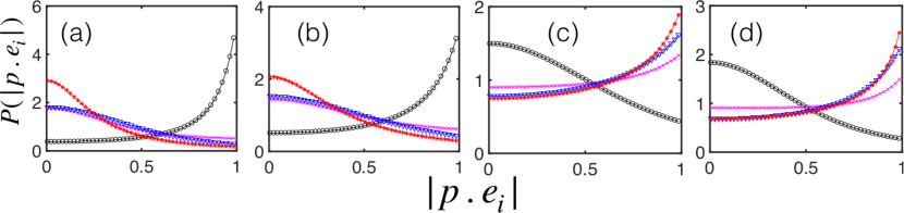
Figure 1: (color online) Representative plots of the probability density function of the alignment of the orientation vector ${\bf p}$ with ${\bf e}_{1}$ (black circle $\circ$), ${\bf e}_{2}$ (pink cross $\times$), ${\bf e}_{3}$ (blue inverted triangle $\triangledown$) and ${\bf e}_{w}$ (red asterisk $\ast$) for (a) $\alpha=0.1$ (oblate), (b) $\alpha=0.5$ (c) $\alpha=1.5$, and (d) $\alpha=2.0$ (rod). These measurements are made for particles with a bare Stokes numbers $St_{\rm s}=1.0$. (In Table 1, the actual Stokes numbers corresponding to the different particles are listed.)

We begin by considering a spheroid of density $\rho_{p}$, with a symmetry axes of length $2c$ and the two equal axis of length $2a$, such that the ratio $\alpha=c/a$ characterizes the nature of the spheroid, moving with a velocity ${\bf v}$, and advected by a carrier fluid with velocity ${\bf u}$. In the most general case, the drag felt by a non-spherical particle is characterized by its resistance tensor $\mathrm{K}$ brenner and the use of quaternion algebra in recent years wachem provides a convenient route to study the problem in its most general setting [see, e.g., Voth and Soldati vothARFM and references therein]. The equations of translational motion of the center of the spheroid ${\bf r}$ are given by the Stokes drag model:

$$\frac{d{\bf r}}{dt}={\bf v};\quad\frac{d{\bf v}}{dt}=-\frac{\mathrm{A}^{\mathrm{T}}\mathrm{K}\mathrm{A}}{6\pi a\alpha}\frac{[{\bf v}-{\bf u}]}{\tau_{s}},$$ (1)

where the carrier fluid velocity ${\bf u}$ above is evaluated at the particle position ${\bf r}$. The Stokes time for a spherical particle of radius $a$ is given by $\tau_{s}=2\rho_{p}a^{2}/9\rho_{f}\nu$, where $\rho_{f}$ is the density and $\nu$ is the kinematic viscosity of the carrier flow. The details of the resistence tensor $\mathrm{K}$ and the orthogonal transformation matrix $\mathrm{A}$ are described in Ref. mortensenPoF08 for prolate spheroids and Ref. challabotlajfm15 for oblate spheroids. The Stokes time $\tau_{p}$, based on isotropic particle orientation and the inverse of the resistance tensor, differs from the more familiar spherical case $\tau_{s}$ to take into account the asymmetry of the particle anderson-prl ,

$$\tau_{p}=\begin{cases}\tau_{s}\frac{\alpha\{\pi-2\tan^{-1}[\alpha({1-\alpha^{2}})^{-1/2}]\}}{2\sqrt{1-\alpha^{2}}}\quad\alpha<1\\ \tau_{s}\frac{\alpha\ln[\alpha+\sqrt{\alpha^{2}-1}]}{\sqrt{\alpha^{2}-1}}\quad\alpha>1.\end{cases}$$ (2)

We see immediately that for $\alpha=1$, which corresponds to a spherical particle since $a=c$, the $\tau_{p}=\tau_{s}$ via the definition above by setting $\alpha=1$. For convenience, we define a bare Stokes number $St_{\rm s}=\tau_{s}/\tau_{\eta}$; the actual Stokes number $St$ will of course depend on the value $\alpha$ via (2); in the spherical case $St\equiv St_{\rm s}$. In Table 1, we list all the values of $\alpha$ and the Stokes numbers that we have used in our simulations.

For asymmetric particles $\alpha\neq 1$, along with the translational motion (defined above), the instantaneous orientation is vital to understand the full dynamics of such spheroids. Intuitively, the direction of the orientation vector ${\bf p}$ for a given spheroid, with a given $\tau_{p}$ and $\alpha$, is determined by the local flow geometry. For a given, generic complex flow, the local geometry is determined by the fluid-velocity-gradient tensor (traceless for incompressible flows), evaluated at the particle position ${\mathcal{A}}_{ij}=\frac{\partial u_{i}}{\partial r_{j}}$. It is useful to split this fluid-velocity-gradient tensor ${\bf\mathcal{A}}={\bf S}+{\bf\Omega}$ into a symmetric part, the strain rate, ${\bf S}^{T}={\bf S}$ and an antisymmetric part, the vorticity tensor, ${\bf\Omega}^{T}=-{\bf\Omega}$. This decomposition is especially useful to write the equation for the orientation vector ${\bf p}$, the so-called Jeffery equation jeffery

$$\frac{d{\bf p}}{dt}={\bf\Omega\,p}+\frac{\alpha^{2}-1}{\alpha^{2}+1}\left[{\bf S\,p}-({\bf p\cdot S\,p})\,{\bf p}\right],$$ (3)

where the strain rate and vorticity tensor are instantaneous measurements at the (inertial) particle position.

It is important to stress that we are approximating the particle dynamics by ignoring the inertia associated with its rotational dynamics. Such a simplification is justified because it has been shown that the typical relaxation timescale associated with the rotational dynamics is an order of magnitude smaller than the $\tau_{p}$ anderson-prl ; marchioli .

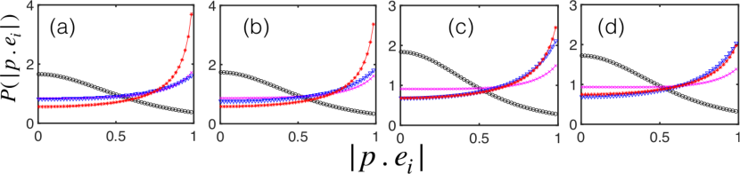
Figure 2: (color online) Representative plots of the probability density function of the alignment of the orientation vector ${\bf p}$ of a rod ($\alpha=2.0$) with ${\bf e}_{1}$ (black circle $\circ$), ${\bf e}_{2}$ (pink cross $\times$), ${\bf e}_{3}$ (blue inverted triangle $\triangledown$) and ${\bf e}_{w}$ (red asterisk $\ast$) for (a) $St=0.0$, (b) $St=0.152$, (c) $St=0.76$, and (d) $St=4.56$.

	0.1	0.5	0.9	1.0	1.1	1.5	2.0
	oblate			sphere			rod
0.0	0.0	0.0	0.0	0.0	0.0	0.0	0.0
0.1	0.015	0.067	0.247	0.1	0.106	0.129	0.152
0.5	0.075	0.34	1.24	0.5	0.53	0.65	0.76
1.0	0.15	0.67	2.47	1.0	1.064	1.29	1.52
2.0	0.30	1.34	4.94	2.0	2.13	2.58	3.04
3.0	0.45	2.01	7.41	3.0	3.19	3.87	4.56

Table 1: Values of the aspect ratios $\alpha$, the bare Stokes numbers $St_{\rm s}$, and the actual Stokes numbers $St$ for the different sets of particles that we have used in our simulations (see text).

We finally turn our attention to the advecting or carrier fluid velocity ${\bf u}$. Since we study the spheroid in a three-dimensional, incompressible turbulent flow, we obtain the velocity field as a solution of the forced three-dimensional Navier-Stokes equation :

$$\frac{\partial{\bf u}}{\partial t}+{\bf u}\cdot{\nabla}{\bf u}=\nu\nabla^{2}{\bf u}-\frac{\nabla P}{\rho_{f}}+{\bf f},$$ (4)

augmented by the incompressibility constraint $\nabla\cdot{\bf u}=0$, where $P$ is the pressure and the forcing ${\bf f}$ drives the system to a statistically steady state. We recall that a three-dimensional turbulent flow are characterised by the Kolmogorov micro-scales for length $\eta=\left(\frac{\nu^{3}}{\epsilon}\right)^{1/4}$, time $\tau_{\eta}=\left(\frac{\nu}{\epsilon}\right)^{1/2}$, and velocity $u_{\eta}=\left(\nu\epsilon\right)^{1/4}$. These definitions allow us in a unique way, which allows a comparison between experiments, numerical simulations, and theory, to define the Stokes number $St=\tau_{p}/\tau_{\eta}$. We should also note that our model, and hence the results, are valid only for $a,c\ll\eta$.

Before we discuss the various results, let us briefly outline the numerical strategy used in our calculations. (We refer the reader to Ref. james for more details.) We solve for the fluid velocity by using the standard pseudo-spectral method with $N^{3}=512^{3}$ collocation points and a second-order Adams-Bashforth scheme to integrate in time. We drive the system to a statistically steady state by using a constant, large-scale energy injection forcing pope-forc ; pandit one to reach the Taylor-scale Reynolds number $Re_{\lambda}\simeq 120$.

To obtain the translational and orientation statistics, we seed the flow (as obtained above) with (non-interacting) particles with seven different values of $0.1\leq\alpha\leq 2$ (including the spherical case $\alpha=1$) and, including the tracers, six different Stokes numbers $0.0\leq St_{\rm s}\leq 3.0$; we use $N_{p}=50000$ particles for each $\alpha-St$ combination. We also run our simulations for several large-eddy-turn-over times to rule out transient effects and obtain well-converged statistics. The trajectories of individual particles are integrated by using a trilinear interpolation scheme  NumRec to obtain the fluid velocity at the particle position. We set up an initial condition for the spheroids such that their orientation vector initially ($t=0$) points along the ${\bf\hat{x}}$ direction.

We begin by examining the alignment of the spheroids as a function of the Stokes number and the aspect ratio. A convenient measure of the flow geometry is to exploit the bases of the symmetric tensor ${\bf S}$ and the anti-symmetric tensor ${\bf\Omega}$. Given the nature of the strain-rate matrix, it is trivial to see that it allows three eigenvalues $\lambda_{1}\geq\lambda_{2}\geq\lambda_{3}$ which correspond to a set of three orthonormal eigenvector basis ${\bf S}{\bf e}_{i}=\lambda_{i}{\bf e}_{i}$. The vorticity tensor is constructed from the vorticity vector ${\bf\omega}$ yielding a unit vector ${\bf e_{\omega}}$ corresponding to the magnitude of the vorticity $\omega$.

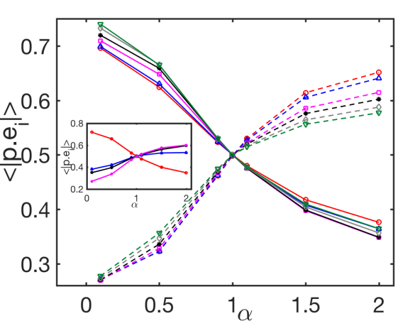
Figure 3: (color online) Plots of (a) $\langle|{\bf p}.{\bf e}_{i}|\rangle$ and (b) $\langle|{\bf p}.{\bf e}_{i}|^{2}\rangle$ vs $\alpha$ for $St_{\rm s}=0$ (red open circles), $St_{\rm s}=0.1$ (blue upward-pointing triangles), $St_{\rm s}=0.5$ (magenta squares), $St_{\rm s}=1.0$ (black asterisks), $St_{\rm s}=1.5$ (gray diamonds), $St_{\rm s}=2.0$ (green downward-pointing triangles). The solid and dashed lines are for ${\bf e}_{1}$ and ${\bf e}_{\omega}$, respectively. The insets show the representative plots of the same quantities, at $St_{\rm s}=1$, for ${\bf e}_{1}$ (red open circles), ${\bf e}_{2}$ (blue triangles), ${\bf e}_{3}$ (black squares), and ${\bf e}_{\omega}$ (magenta asterisks).

We characterize the alignment of the spheroids by calculating the probability distribution function of the cosine of the angle between their orientation vector with the different eigenvectors of the flow field. The equation of motion for the orientation vector suggests that $\bf p$ ought to align preferentially with the principle axis of the strain rate matrix ${\bf e}_{1}$. Surprisingly, however, it was shown by Pumir and Wilkinson wilkinson-NJP , that measurements for tracers are inconsistent with this naïve conclusion. In Fig. 2(a) we confirm this conclusion from our numerical simulations. Given the plausible explanation for this phenomenon wilkinson-NJP , it is important to examine the effect of finite Stokes numbers. This is especially important because inertial spheroids will sample, preferentially, straining regions of the flow.

In Fig. 1, we show representative plots of this probability distribution function, namely $P(|{\bf p}.{\bf e}_{i}|)$ vs $|{\bf p}.{\bf e}_{i}|$, where $i=1,2,3$, and $\omega$, for different values of $\alpha$ (for the same bare Stokes number of unity), calculated at times longer than the initial transient phase (see Fig. 1 in Ref. wilkinson-NJP ). Unlike the tracer case, we see a very different behavior. For inertial oblates [Figs. 1 (a) and (b)], the spheroid tends to preferentially align with the principle axis of the strain rate matrix as we should expect from the equation of motion for the orientation vector. This behaviour is in contrast to rods ($\alpha>1$) as shown in Figs. 1 (c) and (d) where the alignment is most strongly with the vorticity direction ${\bf e}_{\omega}$ as has been known for tracers chevillardjfm . This behavior for rods is completely consistent with what is known for tracer rods wilkinson-NJP and illustrated in Fig. 2(a). However unlike the $St=0$ case, for finite inertia rods tend to align to a greater degree with the non major axes of the strain rate matrix, namely ${\bf e}_{2}$ and ${\bf e}_{3}$. Indeed this effect is enhanced for a given rod ($\alpha=2.0$) with increasing inertia. In Fig. 2 we show representative plots of the probability density function for a rod with increasing values of the Stokes number from Figs. 2 (a) to (d). We clearly see that as the Stokes number increases, rods tend to align more and more with the axis ${\bf e}_{3}$ and, eventually, for the largest Stokes number considered here ($St=4.56$, Fig 2d), the alignment is strongest with ${\bf e}_{3}$ instead of ${\bf e}_{\omega}$ (Fig. 2(a)). For small inertia, rods tend to align with ${\bf e}_{\omega}$; however with increasing translational inertia, these spheroids start preferentially sampling strain-dominated regions. Hence, as the Stokes number increases, the rods start de-aligning with ${\bf e}_{\omega}$ and aligning with the most contracting eigenvector ${\bf e}_{3}$ (as clearly seen in our measurements) because the vorticity is normal to the most contracting direction meneveauARFM .

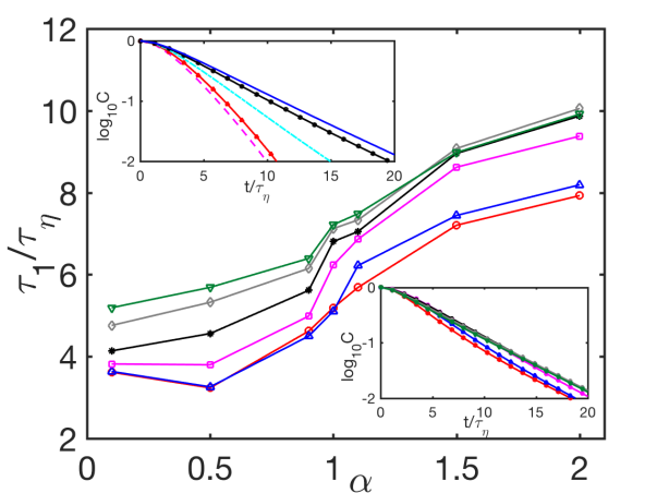
Figure 4: (color online) Plot of characteristic decay times, normalized by $\tau_{\eta}$, of the correlation functions (a) $\langle{\bf p}(t).{\bf p}(0)\rangle$ and (b) $\langle|{\bf p}(t).{\bf p}(0)|\rangle$ vs $\alpha$ for different $St_{\rm s}$. The color codes are the same as in Fig. 3. The top-left insets show the correlation function decay for a fixed $St_{\rm s}=1.0$ and changing $\alpha$ from $\alpha=0.1$ (magenta dashed line), $\alpha=0.5$ (red triangles), $\alpha=1.0$ (cyan dashed-dotted line), $\alpha=1.5$ (black open circles) and $\alpha=2.0$ (blue solid line). The bottom-right insets show the correlation function decay for a fixed $\alpha=2.0$ and different $St_{\rm s}$ (same color code as the main plot). In the y axis of the insets of the left panel $C=\langle{\bf p}(t).{\bf p}(0)\rangle$ and the right panel $C_{\rm abs}=\langle|{\bf p}(t).{\bf p}(0)|\rangle-0.5$.

Our results suggest, unsurprisingly, that the dynamics of oblates, spheres, and rods are qualitatively different from each other. Indeed for spherical particles, we expect that for all Stokes numbers, the orientation vector should rotate randomly, yielding, on average $\langle|{\bf p}.{\bf e}_{i}|\rangle$ = 0.5 and $\langle|{\bf p}.{\bf e}_{i}|^{2}\rangle$ = 0.33. This reasoning breaks down in the case of spheroids; indeed in the limiting case of tracer-rods ($St=0$ and $\alpha\to\infty$), the actual values of these measures are quite far from the spherical case wilkinson-NJP . In order to systematically study the mean orientation of inertial spheroids, we measure $\langle|{\bf p}.{\bf e}_{i}|\rangle$ and $\langle|{\bf p}.{\bf e}_{i}|^{2}\rangle$. In Fig. 3(a) and (b), we show plots of $\langle|{\bf p}.{\bf e}_{i}|\rangle$ and $\langle|{\bf p}.{\bf e}_{i}|^{2}\rangle$, respectively, for ${\bf e}_{1}$ and ${\bf e}_{\omega}$, as a function of the aspect ratio $\alpha$ for a few representative values of the Stokes numbers. For both these measures, the alignment with respect to the principle axis of the strain rate matrix is close to 1 in the limit $\alpha\to 0$ and decreases monotonically and approaches 0 as $\alpha\gg 1$. This behavior is exactly opposite to the mean alignment with respect to the vorticity eigendirection where both these measures increases monotonically with $\alpha$ and saturates, asymptotically, as $\alpha\gg 1$. We note that in the limiting spherical case $\alpha=1$, $\langle|{\bf p}.{\bf e}_{1}|\rangle$ = $\langle|{\bf p}.{\bf e}_{\omega}|\rangle$ = 0.5 and $\langle|{\bf p}.{\bf e}_{1}|^{2}\rangle$ = $\langle|{\bf p}.{\bf e}_{\omega}|^{2}\rangle$ = 0.33 as suggested earlier. Furthermore, we observe that $\langle|{\bf p}.{\bf e}_{\omega}|\rangle$ and $\langle|{\bf p}.{\bf e}_{\omega}|^{2}\rangle$ does not change with St for disks where as they decrease monotonically with St for rods. On the other hand for the case ${\bf e}_{1}$ these measures increase monotonically with St for disks; for the rods, however, this value first decreases with St, reaches a minimum at $\mbox{{St}}=0.5$, and then increases with St. Finally, we note that the mean values for the alignment with ${\bf e}_{2}$ and ${\bf e}_{3}$ are following the same trend as ${\bf e}_{1}$ as shown in the insets of Fig 3.

Although it is still difficult in an experiment to accurately measure the different eigenvectors along the Lagrangian trajectory of an spheroid – as we have done above – a surrogate measurement is the autocorrelation functions $C\equiv\langle({\bf p}(t).{\bf p}(0))\rangle$, $C_{\rm abs}\equiv\langle|{\bf p}(t).{\bf p}(0)|\rangle$ and $C_{2}\equiv\langle|{\bf p}(t).{\bf p}(0)|^{2}\rangle$ which decay exponentially at short times. At long times, these correlations asymptote to values close to 0, 0.5 and 0.33, respectively as discussed above. We measure such correlation functions and extract the characteristic decay time scales $\tau_{1}$, $\tau_{2}$, and $\tau_{3}$ associated with each of these correlation functions. In Fig. 4 we show representative plots of $\tau_{1}$ [Fig. 4(a)] and $\tau_{2}$ [Fig. 4(b)], normalized by the Kolmogorov time-scale $\tau_{\eta}$, as a function of the aspect ratio $\alpha$ for a few representative values of the Stokes numbers. These results are consistent for the case of oblates studied (for similar inertia and aspect ratios)by Jucha, et al. jucha as well as converging to the rod- and tracer-limits reported in Ref. wilkinson-NJP .

Our measurements show a monotonic increase with the aspect ratio $\alpha$ with a mild, but non-trivial, dependence on the level of inertia. For $\alpha=0.1$ (disks), $\tau_{1}$ increases monotonically with an increase in St, but for the largest simulated $\alpha=2$, case first $\tau_{1}$ increases reaches a maximum at $\mbox{{St}}=1$ and saturates with increasing St. We note that the maximum characteristic time for $\alpha=2$ (rods) reaches at $\mbox{{St}}=1$, which corresponds to the case where maximum clustering starts to happen in turbulent flow.

For spherical particles, $\alpha=1$, the second term on the right-hand-side of Eq. (3) is absent by definition. Hence for spherical particles, the characteristic time scale is set by $\Omega$. However, assuming the term $\left({\bf S\,p}-({\bf p\cdot S\,p})\,{\bf p}\right)$ to be positive definite, a naïve interpretation of Eq. 3 suggests that for $\alpha<1$, the time scales for disks ought to be less than those for spheres; similarly for $\alpha>1$, the time scales for rods should be larger than those for spheres. This interpretation is consistent with the numerical results reported in Fig. 4. More pertinently, the statistics of alignment (discussed above) suggests that, for example, for disks, inertia leads to the orientation vector being orthogonal, preferentially, to the vorticity of the flows which lie in the plane of the disk, and hence, to a faster rotation of the orientation vector. Such an argument suggests that oblates rotate faster than rods resulting in a smaller decorrelation time for oblates than for rods. With increasing inertia, however, there is a preferential sampling of strain-dominated regions by particles of all shapes. Hence this leads, inevitably, to a smaller rotation rate and hence a larger decorrelation time. Indeed our measurements (Fig. 4) show this to be the case. For the extremal values of $\alpha$, namely $\alpha=0.1$ and $\alpha=2.0$, the maximum values of St are 0.45 and 4.56, respectively. Hence we find that the decorrelation times for oblates are monotonically increasing in time with the Stokes number whereas for rods the saturation behavior is consistent with the fact that significant clustering starts to take place after $\mbox{{St}}>1$. It is important to stress that these arguments are far from rigorous but seems to be consistent with our observations.

The rotational dynamics of small, but non-spherical, particles in turbulent flows is an important problem in many areas of fluid mechanics. In recent years, because of all the reasons mentioned earlier, there has been a lot of work in this area. However by and large most numerical and theoretical efforts have tended to ignore the effect of inertia – and hence preferential sampling of the fluid velocity – on the alignment properties of such particles. Furthermore even for the tracer case most studies have typically concentrated on the problem of rods. In this Rapid Communication, we have therefore systematically studied this problem by including the effects of inertia, for a large interval of aspect ratios spanning both disks and rods, to elucidate the statistics of the directional vector with respect to the geometry of the advecting flow. Our results show that the case of tracer rods, studied earlier, is a special case of spheroids and does not easily generalize for finite Stokes numbers or for disks. An important implication of our results lie in the modeling of asymmetrical microorganisms and the emergence of collective behavior (under suitable interactions) in a flow unpublished .

- (1) M. R. Maxey and J. J. Riley, Physics of Fluids 26, 883 (1983).
- (2) J Bec, Phys. Fluids 15, L81-L84 (2003); J. Bec, J. Fluid Mech. 528, 255 (2005)
- (3) E. W Saw, G. P. Bewley, E. Bodenschatz, S. S. Ray, J. Bec, Phys. Fluids 26, 111702 (2014)
- (4) G. Falkovich, A. Fouxon, and M. Stepanov, Nature 419, 151-154 (2002).
- (5) M. Wilkinson, B. Mehlig, and V. Bezuglyy, Phys. Rev. Lett. 97, 048501 (2006).
- (6) K. Gustavsson and B. Mehlig, Phys. Rev. E 84, 045304 (2011).
- (7) J. Bec, H. Homann, and S. S. Ray, Phys. Rev. Lett. 112, 184501 (2014).
- (8) J. Bec, S. S. Ray, E.-W. Saw, and H. Homann, Phys. Rev. E 93, 031102(R) (2016).
- (9) T. J. Pedley and J. O. Kessler, Annu. Rev. Fluid Mech. 24, 313 (1992); D. Saintillan and M.J. Shelley, Phys. Rev. Lett. 99, 058102 (2007).
- (10) A. Choudhary, D. Venkataraman, and S. S. Ray, Europhys. Lett., 112, 24005 (2015).
- (11) M. B. Pinsky and A. P. Khain, Atmos. Res. 47-48, 69 (1998); S. C. Sherwood, V. T. J. Phillips, and J. S. Wettlaufer, Geophys. Res. Lett. 33, L05804 (2006).
- (12) A. J. Szeri, W. J. Milliken, and L. G. Leal, J. Fluid Mech. 237, 33 (1992); M. Wilkinson, V. Bezuglyy, and B. Mehlig, Phys. Fluids 21, 043304 (2009); E. Gavze, M. Pinsky, and A. Khain, J. Fluid Mech. 690, 51 (2011); V. Dabade, N. K. Marath and G. Subramanian, J. Fluid Mech. 791, 631 (2016); N. K. Marath and G. Subramanian, J. Fluid Mech. 844, 357 (2018).
- (13) S. Parsa, J. S. Guasto, M. Kishore, N. T. Ouellette, J. P. Gollub, and G. A. Voth, Phys. Fluids 23, 043302 (2011).
- (14) S. Parsa, E. Calzavarini, F. Toschi, and G. A. Voth Phys. Rev. Lett. 109, 134501 (2012).
- (15) H. Zhang, G. Ahmadi, F.-G. Fan, and J. B. McLaughlin, Int. J. Multiphase Flow 27, 971 (2001); C. Marchioli, M. Fantoni, and A. Soldati, Phys. Fluids 22, 033301 (2010); L. Zhao, C. Marchioli, and H. I. Andersson, Phys. Fluids 26, 063302 (2014); C. Marchioli and A. Soldati, Acta Mech. 224, 2311 (2013).
- (16) P. H. Mortensen, H. I. Andersson, J. J. J. Gillissen, and B. J. Boersma, Phys. Fluids 20, 093302 (2008);
- (17) C. Siewert, R. P. J. Kunnen, M. Meinke, and W. Schröder, Atmos. Res. 142, 45 (2014).
- (18) K. Gustavsson, J. Jucha, A. Naso, E. Lévêque, A. Pumir, and B. Mehlig, Phys. Rev. Lett. 119, 254501 (2017).
- (19) J. Jucha, A. Naso, E. Lévêque, and A. Pumir, Phys. Rev. Fluids 3, 014604 (2018).
- (20) G. Bellani, M. L. Byron, A. G. Collignon, C. R. Meyer, and E. A. Variano, J. Fluid Mech. 712, 41 (2012).
- (21) L. Chevillard and C. Meneveau, J. Fluid Mech. 737, 571 (2013).
- (22) K. Gustavsson, J. Einarsson, and B. Mehlig, Phys. Rev. Lett. 112, 014501 (2014).
- (23) A. Pumir and M. Wilkinson, New J. Phys. 13 093030 (2011).
- (24) A. Gupta, D. Vincenzi and R. Pandit, Phys. Rev. E 89 021001(R) (2014).
- (25) L. Zhao, N. R. Challabotla, H. I. Andersson, and E. A. Variano, Phys. Rev. Lett. 115, 244501 (2015).
- (26) H. Brenner, Chem. Eng. Sci. 19, 703 (1964).
- (27) F. Zhao and B. G. M. van Wachem, Acta Mech. 224, 3091 (2013).
- (28) G. A. Voth and A. Soldati, Ann. Rev. Fluid Mech. 49, 249 (2017).
- (29) N. R. Challabotla, L. Zhao, and H. I. Andersson, J. Fluid Mech. 766, R2 (2015).
- (30) G. B. Jeffery, Proc. R. Soc. A 102, 161 (1922).
- (31) C. Marchioli, L. Zhao, and H. I. Andersson, Phys. Fluids 28, 013301 (2016).
- (32) M. James and S. S. Ray, Sci. Rep. 7, 12231 (2017).
- (33) A.G. Lamorgese, D.A. Caughey, and S.B. Pope, Phys. Fluids 17, 015106 (2005).
- (34) G. Sahoo, P. Perlekar, and R. Pandit, New J. Phys. 13, 0130363 (2011).
- (35) W. H. Press, Numerical Recipes 3rd Edition: The Art of Scientific Computing (Cambridge University Press, Cambridge, United Kingdom, 2007).
- (36) C. Meneveau, Ann. Rev. Fluid Mech. 43, 219 (2011).
- (37) A. Gupta, A. Roy, A. Saha, and S. S. Ray, in preparation.