Modelling Non-Markovian Quantum Processes with Recurrent Neural Networks

Abstract

Quantum systems interacting with an unknown environment are notoriously difficult to model, especially in presence of non-Markovian and non-perturbative effects. Here we introduce a neural network based approach, which has the mathematical simplicity of the Gorini-Kossakowski-Sudarshan-Lindblad master equation, but is able to model non-Markovian effects in different regimes. This is achieved by using recurrent neural networks for defining Lindblad operators that can keep track of memory effects. Building upon this framework, we also introduce a neural network architecture that is able to reproduce the entire quantum evolution, given an initial state. As an application we study how to train these models for quantum process tomography, showing that recurrent neural networks are accurate over different times and regimes.

I Introduction

Traditionally, in the physical sciences, the study of mathematical problems for which no analytic solution is available involves modelling methods leveraging a combination of approximation techniques (such as perturbation theory or semiclassical approaches) and the use of symmetries to reduce the complexity of the problem. Recently, advances in machine learning Bishop (2006); LeCun et al. (2015), have caused a surge in popularity of data-driven approaches, which instead rely on computational techniques that exploit statistical correlations. Applications range from chaos theory Pathak et al. (2018) to high energy physics Komiske et al. (2017), eventually showing many applications and new perspectives in the quantum domain Schuld et al. (2015); Biamonte et al. (2017); Ciliberto et al. (2018); Dunjko and Briegel (2018). In particular, artificial neural networks (a class of learning methods inspired by the functioning of the brain) have been utilized in quantum many-body physics for ground state estimation Carleo and Troyer (2017), quantum state tomography Torlai et al. (2018); Yu et al. (2018), classification of phases of matter van Nieuwenburg et al. (2017), entanglement estimation Gray et al. (2018), and to identify phase transitions Carrasquilla and Melko (2017). Although the theoretical understanding of the effectiveness of these models is currently limited, some recent papers have established connections between neural networks and more standard frameworks such as renormalization group Mehta and Schwab (2014), tensor networks Levine et al. (2017, 2018); Chen et al. (2018), and complexity theoretic tools Rocchetto et al. (2018). Moreover, classical optimization techniques borrowed from supervised machine learning have been employed to optimize the dynamics of many-body systems Banchi et al. (2016); Innocenti et al. (2018); Eloie et al. (2018); Las Heras et al. (2016); Zahedinejad et al. (2016) and parametric quantum circuits Verdon et al. (2018); Grant et al. (2018); Melnikov et al. (2018); Huggins et al. (2018); Benedetti et al. (2018); Bukov et al. (2018); Niu et al. (2018).

Open quantum systems Breuer and Petruccione (2002); Rivas and Huelga (2012) present further challenges. Here, any modelling effort must take into account that the system interacts with a surrounding environment, whose microscopic details are usually unknown. The resulting effects can only be treated phenomenologically and significantly increase the complexity of the model, especially in the non-Markovian regime. In this regime, exact non-perturbative master equations Ishizaki and Fleming (2009) or quantum maps Pollock et al. (2018) operate by entangling the system with ancillary degrees of freedom whose dimension grows with time. This makes exact simulations extremely challenging even for low dimensional Hilbert spaces. Therefore, in larger systems, non-Markovian effects can only be modelled in an approximate fashion, e.g. by neglecting quantum correlations or by assuming weak couplings between system and environment. When these approximations are justified, phenomenological models with a reduced number of parameters are normally accurate. However, these approximations are often violated, e.g., in quantum biology Ishizaki and Fleming (2009), so it is important to study alternative mathematical structures.

Machine learning methods offer new ideas for modelling non-Markovian effects when standard assumptions do not hold. The intuition behind these approaches is that, if there exists an efficient description of the system, this can be learnt from data without using explicit modelling assumptions. In particular, neural networks based learning techniques have shown that it is possible to learn complex functional dependencies in time series directly from the data, without trying to make theoretical assumptions that may be unjustified (such as the weak coupling limit) or hard to derive from phenomenological observations. In order for these methods to succeed, it is crucial to define the correct neural network structure that can quickly learn the underlying rule to reproduce the unknown functional form displayed in the data.

Here we investigate the ability of neural networks to model the non-Markovian evolution of open quantum systems, using a fixed number of parameters that does not grow with the number of time steps. We focus on Recurrent Neural Networks (RNNs), a type of artificial neural network specifically designed to model dynamical systems with possibly long range temporal correlations. In the quantum setting, RNNs have been previously employed for quantum control August and Ni (2017); Ostaszewski et al. (2018). We consider two main applications. In the first one, we define a master equation which has the mathematical simplicity of the Gorini-Kossakowski-Sudarshan-Lindblad master equation Gorini et al. (1976); Lindblad (1976), but is nonetheless able to model non-Markovian effects via the memory cells included in RNNs. In the second application, we define an RNN able to reproduce the entire quantum evolution given an initial state, without introducing any master equation. Our RNN-based frameworks share some similarity with collisional models Ciccarello et al. (2013); Ziman et al. (2002); Giovannetti and Palma (2012); Rybár et al. (2012); McCloskey and Paternostro (2014); Ciccarello (2017); Campbell et al. (2018) or $\epsilon$-machines Binder et al. (2018), where explicit memory effects are introduced by using ancillary quantum systems. However, there are notable differences. One of the advantages of RNNs is in their ability to learn directly from data how to compress complex time series with a few constant parameters. Moreover, there are different RNN architectures and it is possible to select the most appropriate one to model the expected long-range memory in the time evolution.

We will show that RNNs provide a convenient mathematical framework to define the so-called memory kernel Breuer and Petruccione (2002), such that the resulting time-local master equation has a completely positive solution. The reconstruction of the memory kernel from quantum state sequences, namely from quantum process tomography, has been the subject of different studies in recent years Cerrillo and Cao (2014); Pollock and Modi (2017); Pollock et al. (2018); Howard et al. (2006); Yuen-Zhou et al. (2011); Bellomo et al. (2010). Most approaches considered in the literature start with some assumptions on the microscopic model, and then fits the free parameters given the experimental data. These assumptions are required to avoid having an exponentially growing number of free parameters for increasing number of time steps. However, these assumptions are normally uncontrollable, especially when the details of the microscopic model are unknown. Our main result is to show that RNN-based quantum processes and master equations are able to learn efficient representations of non-Markovian quantum evolutions directly from data sequences and without making any assumption on the underlying physical model. Indeed, even the Hamiltonian of the system can be learnt during this process. Note that, while the Hamiltonian can be learnt with alternative methods, e.g. Bayesian inference Wiebe et al. (2014), the memory kernel is much more difficult, as its functional form, beyond the perturbative regime, is unknown. The main use of RNNs is therefore as a “compression” method, to effectively model complex quantum correlations between system and environment with a constant and fixed number of parameters. As a relevant application for our technique, we consider quantum process tomography and show that RNNs are able to model the physical evolution of quantum systems over different regimes.

The paper is structured as follows. In Sec. II we present relevant technical background. Specifically, in Sec. II.1 we introduce non-Markovian quantum processes and common master equations to describe them. In Sec. II.2 we introduce the RNN architecture employed in this paper. The main ideas are presented in Sec. III, where we introduce our RNN-based master equation (Sec. III.1) and RNN-based quantum process (Sec. III.2), with applications for process tomography (Sec. III.3). Numerical experiments are presented in Sec. IV and conclusions are drawn in Sec. V.

II Background

II.1 Non-Markovian processes

Quantum systems, even the purest ones, are inevitably in contact with an environment. Because of this normally unknown interaction, quantum evolution deviates from the predictions of the Schrödinger equation, and different extensions have been proposed Breuer and Petruccione (2002); Breuer et al. (2016). When the interactions inside the environment happen on timescales much shorter than the internal timescales of the system, then a Markovian approximation is usually appropriate, and the evolution can be modeled via the Gorini-Kossakowski-Sudarshan-Lindblad (GKSL) master equation Gorini et al. (1976); Lindblad (1976)

$$\frac{\partial\rho(t)}{\partial t}= \mathcal{L}[\rho(t)]~{},$$ (1)

$$\mathcal{L}[\rho]= {-}i[H,\rho]+\sum_{\mu}\left[L_{\mu}\rho L_{\mu}^{\dagger}-\frac{1}{2}\left\{L_{\mu}^{\dagger}L_{\mu},\rho\right\}\right]~{},$$

where $H$ is the Hamiltonian, which models the noise-free case, and $L_{\mu}$ are called Lindblad operators. The superoperator $\mathcal{L}$ is called Liouvillian. Mathematical properties of the above equation are well understood Rivas and Huelga (2012). For any choice of $H$ and $L_{\mu}$ the solution of the master equation $\mathcal{E}_{t}=e^{\mathcal{L}t}$ defines a completely positive trace preserving linear map, and is thus a mathematically well-posed mapping between states to states. With properly chosen Lindblad operators, the above master equation models the most general Markovian evolution Gorini et al. (1976); Lindblad (1976). However, the Markovian approximation is not accurate in many situations, for instance when the interactions inside the environment have comparable strengths to the interactions inside the system Ishizaki and Fleming (2009); Banchi et al. (2013). In that case the master equation has to be modified to take into account non-Markovian effects. One of the first and most accurate descriptions of non-Markovian evolution is the Nakajima-Zwanzig (NZ) master equation Breuer and Petruccione (2002)

$$\frac{\partial\rho(t)}{\partial t}={-}i[H,\rho(t)]+\int_{0}^{t}ds\,\mathcal{K}^{\rm NZ}_{t-s}[\rho(s)]+\mathcal{I}(t)~{},$$ (2)

where $\mathcal{K}^{NZ}_{t}$ is a super-operator, the so-called memory kernel, which describes the interaction with the environment, while $\mathcal{I}(t)$ is due to the initial correlations between system and environment. If system and environment are initially uncorrelated, then $\mathcal{I}(t)=0$ for all $t$. It is clear that the above equation describes non-Markovian processes, because the state at time $t+dt$ depends not only on $\rho(t)$ but also on the states $\rho(s)$ for $s<t$. The Nakajima-Zwanzig equation is at the basis of powerful Green function methods to study the spectral properties of the system Mukamel (1999); Zhang et al. (2012); Jang and Silbey (2003); Banchi et al. (2013), since the convolution disappears in the frequency domain. On the other hand, in the time domain the above equation is not easy to solve numerically. To avoid this problem, a different but equally accurate master equation has been proposed, the so-called time-convolutionless (TCL) master equation Breuer and Petruccione (2002), which reads

$$\frac{\partial\rho(t)}{\partial t}={-}i[H,\rho(t)]+\int_{0}^{t}ds\,\mathcal{K}^{\rm TCL}_{t-s}[\rho(t)]+\mathcal{I}(t)~{}.$$ (3)

The main formal difference between Eq. (3) and Eq. (2) is that the whole history of states is fed into the NZ master equation, while in the TCL case the master equation explicitly depends on $\rho(t)$ only, and all non-Markovian effects are included into the memory kernel. As such, the non-Markovian nature of the process resulting from Eq. (3) is less obvious, but it is known that both NZ and TCL master equations can describe the same processes. Indeed, there are formal mappings between $\mathcal{K}^{\rm NZ}$ and $\mathcal{K}^{\rm TCL}$ such that both Eq. (3) and Eq. (2) produce the same physical evolution Chruściński and Kossakowski (2010); Breuer and Petruccione (2002).

Although TCL master equations are relatively easy to solve numerically, the main problem is that the interaction with the environment is normally unknown. In other terms, while $H$ is typically well characterized experimentally, the memory kernel depends on environmental quantities such as the temperature, but also on the spectral properties of the environment which are normally unknown. Non-linear spectroscopy can be used to find the spectral density Mukamel (1999), but the latter does not completely characterizes the memory kernel, without introducing further assumptions. The most commonly employed approximation is the assumption of a weak coupling between system and environment, such that the memory kernel can be formally obtained using perturbation theory. However, there are cases where these approximations are not justified, e.g. in quantum biology Ishizaki and Fleming (2009), where the strength of the interaction with the environment is comparable with the internal interactions inside the system. To go beyond perturbation theory, we introduce then a RNN-based non-Markovian quantum process, where memory effects can be learnt directly from data.

II.2 Recurrent Neural Networks

RNNs are a class of neural networks designed to model data sequences like time series Schmidhuber (2015). To understand their functioning, it is helpful to compare them with more standard feedforward networks. In feedfordward neural networks the input data $s^{0}$ propagates throughout many intermediate (hidden) layers before reaching the final output layer. Here “propagate” means that, step by step, the state $s^{\ell+1}$ of the $(\ell{+}1)$-th layer is updated, given the state of $\ell$-th layer, as $s^{\ell+1}=f(W^{\ell}s^{\ell}+w^{\ell})$ where $W^{\ell}$ is a weight matrix, $w^{\ell}$ a weight vector and $f$ is some non-linear function. The state at the final layer of the network (output layer) depends on all the weight matrices and vectors. Training is performed by updating those weights such that the neural network learns some desired input-output relationship hidden in the data.

In case of temporal data, each input has also an explicit time dependence $s^{0}_{t}$. Although, in principle, one could still use a giant feedforward network with these data, this is rarely the optimal choice, because the number of free parameters quickly increases with the number of time steps. RNNs solve this issue with a more advanced architecture which is tailored for temporal data. In RNNs, the update rule for the hidden layers at time $t$ not only depends on the states $s^{\ell}_{t}$, but also on the states at previous times. In other terms, the update rule is $s^{\ell+1}_{t}=f(W^{\ell}s^{\ell}_{t}+w^{\ell},s^{\ell+1}_{t{-}1})$, where $s^{0}_{t}$ is the input temporal sequence. The free parameters $W^{\ell}$ and $w^{\ell}$ do not depend on $t$, and memory of the past is taken into account by the function $f$, which compresses and saves relevant informations of previous sequences into memory cells. This architecture allows RNNs to learn temporal sequences using a relatively small number of parameters, even when the temporal data has long-range memory effects. The mapping between $s^{\ell}_{t}$ and $s^{\ell+1}_{t}$ defines a RNN cell.

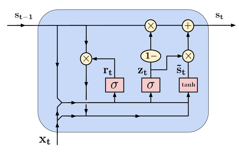
Figure 1: Network diagram of the GRU cell . The output $s_{t}$ and input $s_{t-1}$ represent the state at times $t$ and $t-1$, respectively, while $x_{t}$ is an auxiliary input that depends on the previous times, before $t-1$. Rectangles represent neural network layers. Circles represent entry-wise operations. Bifurcations represent copy operations and joined lines represent concatenation. Details are presented in Appendix A.

In this work we use a variant of RNN called Gated Recurrent Unit (GRU), whose basic cell is shown in Fig. 1 and discussed in Appendix A. GRUs use a gating mechanism that allows them to better model long-term dependencies than more simple RNNs Cho et al. (2014). GRUs are based on a type of RNN cell called Long Short-Term Memory (LSTM), but can be more efficient than LSTMs for comparable performance Hochreiter and Schmidhuber (1997); Chung et al. (2014). GRU and LSTM are commonly used and achieve state of the art performance for sequence modelling across multiple domains, including machine translation, image captioning and forecasting Lipton et al. (2015).

The GRU state $s_{t}$ is a linear interpolation of the previous state $s_{t-1}$ and a candidate state $\tilde{s}_{t}$, which depends on the auxiliary input $x_{t}$. The input $x^{j}_{t}$ for a depth $j$ cell at time $t$ is the state from the cell in the previous layer $s^{j-1}_{t}$. GRU cells can be stacked to form a deep GRU network. More details can be found in Appendix A.

III Main idea

In this section we present the three main contributions of this paper which all leverage on the modelling capabilities of RNNs to describe non-Markovian dynamics of open quantum systems. First, we describe a master equation approach. Second, we use RNNs to predict the time evolution of quantum state under a non-Markovian quantum process. Third, we show how these two techniques can be utilized to perform quantum process tomography.

III.1 RNN Quantum Master Equation

We postulate a quantum evolution similar to Eq. (1), namely

$$\frac{\partial\rho(t)}{\partial t}=\mathcal{L}_{{\leq}{t}}[\rho(t)]~{},$$ (4)

where the notation ${\leq}t$ refers to a superoperator that not only depends on $t$, but also on the entire history before time $t$, as in the TCL master equation (3). A convenient choice is then that of the GKSL form

$$\mathcal{L}_{{\leq}t} [\rho]={-}i[H+H^{LS}_{{\leq}t},\rho]+$$ (5)

$$+\sum_{\mu}\left[L^{\mu}_{{\leq}t}\rho L_{{\leq}t}^{\mu\dagger}-\frac{1}{2}\left\{L_{{\leq}t}^{\mu\dagger}L_{{\leq}t}^{\mu},\rho\right\}\right]~{},$$ (6)

where $H^{LS}$ is a “Lamb-shift” term, namely a correction to the Hamiltonian induced by the environment, while $L^{\mu}$ are Lindblad operators. The reason for this choice is that for small enough $\Delta_{t}$ the time evolution is simply given by $\rho(t+\Delta_{t})\approx e^{\Delta_{t}\mathcal{L}_{{\leq}{t}}}[\rho(t)]~{}$, and since $\mathcal{L}_{{\leq}t}$ is in the GKSL form, $e^{\Delta_{t}\mathcal{L}_{{\leq}t}}$ is a completely positive trace preserving quantum channel, mapping states to states. If $H^{LS}$ and $L^{\mu}$ are simply time-dependent functions, namely they only depend on $t$ and not on previous times, then the dynamics generated by above master equation is always Markovian Chruściński and Kossakowski (2010). The main idea of this work is to use a RNN to define each Lindblad operator $L_{{\leq}t}^{\mu}$ and the correction Hamiltonian $H^{LS}_{{\leq}t_{j}}$, see fig. 2(a). In order to ensure the Hermiticity of the $H^{LS}_{{\leq}t}$ operator, we construct it as $H^{LS}_{{\leq}t}=A(t_{j})+A(t_{j})^{\dagger}$, where $A(t_{j})$ is the output of the network and $A(t_{j})^{\dagger}$ its conjugate transpose. Since in RNNs the predicted output at time $t$ depends on the entire history at previous times, this parametrization is expected to accurately reproduce genuinely non-Markovian effects, even with possible long-range dynamical correlations. The master equation then resembles a TCL master equation (3), but where the complicated memory superoperator is expressed via a simpler GKSL form with RNNs. We call our Eq. (5) the Quantum Recurrent Neural (QRN) Master Equation. Similarly, we call the operators $L_{{\leq}t}^{\mu}$ recurrent Lindblad operators. A schematics of the resulting neural network is shown in Fig. 2(a).

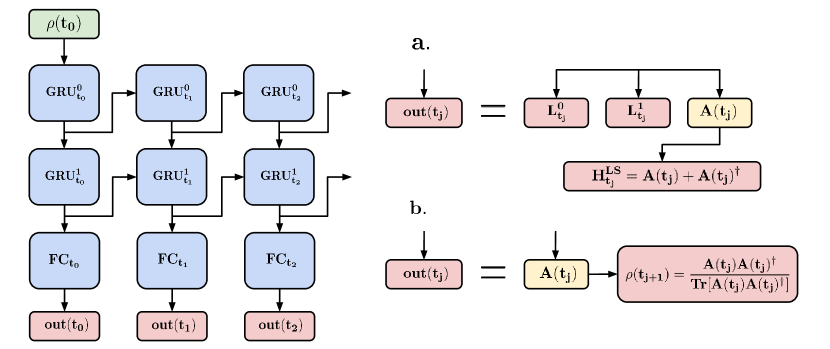
Figure 2: RNN architectures for open quantum systems: schematic of a one-to-many deep RNN used to approximate the master equation and to model the non-Markovian dynamics. Both networks take as input $\rho(t_{0})$ (green cell) and comprise of two GRU layers and a fully connected (FC) layer (blue cells). The yellow cells show the initial network output $A(t_{j})$ before the post-processing that makes $H_{t_{j}}^{LS}$ Hermitian and $\rho(t_{j+1})$ a valid density operator. Panel a. shows the output for the QML master equation, i.e. the predicted value of $H^{LS}_{t}$ and $L^{\mu}_{t}$ at intervals $\Delta{t}$ (red cells). Panel b. shows the output for a RNN modelling the time evolution of a quantum state undergoing a non-Markovian quantum process, i.e. the predicted value of $\rho(t)$ at intervals $\Delta{t}$ (red cells).

III.2 RNN Quantum Processes

For any initial time $t_{0}$ the mapping between the initial state $\rho(t_{0})$ and the state at time $t$, namely

$$\rho(t)=\mathcal{E}(t,t_{0})[\rho(t_{0})]~{},$$ (7)

defines a completely positive map, assuming no initial correlation with the environment. For any intermediate times $t_{0}<\tau<t$ the mapping $\mathcal{E}(\tau,t_{0})$ is always completely positive. When also $\mathcal{E}^{\prime}(t,\tau):=\mathcal{E}(t,t_{0})\mathcal{E}(\tau,t_{0})^{-1}$ is completely positive, then the mapping is called divisible Vacchini et al. (2011). Divisibility is another way of characterising Markovianity, as quantum processes obtained from the GKSL master equation are always divisible with $\mathcal{E}(t^{\prime},t)=\mathcal{T}\exp\left(\int_{t}^{t^{\prime}}\mathcal{L}_{s}\,ds\right)$.

In the previous section we have introduced the QRN master equation and shown that it can model non-Markovian effects, even when the evolution between intermediate steps is completely positive. This is possible because the RNN keeps a compressed record of the previous evolution. Using the formalism of the previous section we can indeed write

$$\mathcal{E}(t,t_{0})=\overleftarrow{\prod_{j}}\mathcal{E}^{QRN}(t_{j}+\Delta_{t},t_{j})+\mathcal{O}(\Delta_{t}^{-2}),$$ (8)

where $\overleftarrow{\prod}_{j}X_{j}$ is the ordered product $\cdots X_{3}X_{2}X_{1}$. Moreover,

$$\mathcal{E}^{QRN}(t_{j}+\Delta_{t},t_{j})=e^{\Delta_{t}\mathcal{L}_{{\leq}{t_{j}}}}$$ (9)

is completely positive, being the operator exponential of a Liouvillian, but depends on the previous evolution, via the recurrent Lindblad operators. As such, the total map (8) is not divisible.

Based on this analogy, we can now drop the master equation and define a non-Markovian process as

$$\mathcal{E}(t,t_{0})=\overleftarrow{\prod_{j}}\mathcal{E}^{RNN}_{{\leq}t_{j}}(t_{j+1},t_{j})~{},$$ (10)

where $\mathcal{E}^{RNN}_{{\leq}t_{j}}(t_{j+1},t_{j})$ is completely positive, but depends on the entire history before $t_{j}$. Each $\mathcal{E}^{RNN}_{{\leq}t_{j}}(t_{j+1},t_{j})$, being completely positive, outputs a valid quantum state at intermediate times $\rho(t_{j})$ and, being a RNN, then updates its internal memory. Complete positivity can be ensured by using the Kraus decomposition or the environmental representation.

For better comparison with the QRN master equation, in this work we use the simpler strategy shown in Fig. 2(b), where we use the output $A(t_{j})$ of the network to define a density operator via $\rho(t_{j+1})=A(t_{j})A(t_{j})^{\dagger}/\operatorname{Tr}[A(t_{j})A(t_{j})^{\dagger}]$. This ensures that the states $\rho(t_{j})$ are valid density operators, throughout the entire evolution.

III.3 Application: Quantum Process Tomography

In this work we apply our QRN master equations and RNN quantum processes for quantum process tomography. We consider the following setup. We assume that the quantum system can be initialized in different initial states $\rho_{\alpha}(0)$ where $\alpha=1,\dots,N_{\mathrm{I}}$, for some number $N_{\mathrm{I}}$. For each initialization, we assume that it is possible to perform full-quantum tomography at some time steps $0\leq t_{j}\leq T$ for $j=1,\dots,N_{\mathrm{T}}$ and some $N_{\mathrm{T}}$. After this procedure we are able to reconstruct the time evolutions $\rho_{\alpha}(t_{j})$ for different times and initializations. Here we consider uniformly separated times where $t_{j}=j\Delta_{T}$ and $\Delta_{T}=T/N_{\mathrm{T}}$, though it is straightforward to generalize this procedure to non-uniform sequences. Each state tomography requires $\mathcal{O}(d^{2})$ measurements, where $d$ is the dimension of the system’s Hilbert space, so the total cost of reconstructing these sequences is $\mathcal{O}(d^{2}N_{\mathrm{T}}N_{\mathrm{I}})$. Once these sequences are obtained, we use them to train the neural network.

We consider two cases. In the first one we train a RNN to learn the quantum state evolution, as shown in Fig. 2(b). Here we assume no knowledge about the system’s Hamiltonian or interaction with the environment. Training is then performed by minimising a cost function

$$J_{p}=\frac{1}{N_{\mathrm{I}}N_{\mathrm{T}}}\sum_{\alpha=1}^{N_{\mathrm{I}}}\sum_{j=1}^{N_{\mathrm{T}}}\|\rho_{\alpha}(t_{j})-\tilde{\rho}_{\alpha}(t_{j})\|~{},$$ (11)

where $\rho_{\alpha}(t_{j})$ are the training data, $\tilde{\rho}_{\alpha}(t_{j})$ are the states outputted by the RNN, and $\|\cdot\|$ is any operator norm.

In the second application we aim at reconstructing $H^{LS}_{{\leq}t}$ and the recurrent Liouvillian operators $L^{\mu}_{{\leq}t}$ entering in the QRN master equation, where, on the other hand, we assume that the Hamiltonian $H$ is known. The latter assumption can always be relaxed, as Hamiltonian evolution can be fully included into the correction Hamiltonian $H^{LS}$, which is learnt from the data. In the QRN master equation, the operators $H^{LS}_{{\leq}{t}}$ and $L^{\mu}_{{\leq}{t}}$ are obtained from the output of the RNN, as shown in Fig. 2(b). To train the RNNs to predict $H^{LS}$ and $L^{\mu}$ given a starting state $\rho_{\alpha}(t=0)$ we propose the use of the differential equation (4) to define a cost function. For classical time series, a similar approach Schmidt and Lipson (2009) has been employed for extracting natural laws from experimental data.

To explain our idea, let us first consider the opposite scenario, where the differential equation (4), with all of its operators, is already known, while the states $\rho(t_{j})$ are not. In this common case, the states $\rho(t_{j})$ at different times are evaluated from the numerical integration of the master equation. The latter can be obtained with an $n$-order Runge-Kutta integrator Süli and Mayers (2003) which, in general, can be formally written as

$$\rho_{\alpha}(t_{j+1})=\rho_{\alpha}(t_{j})+\Delta_{T}\mathcal{L}^{{\rm RK},n}_{{\leq}t_{j}}[\rho_{\alpha}(t_{j})]~{},$$ (12)

where $\mathcal{L}^{{\rm RK},n}_{{\leq}t}$ is $n$-th order Runge-Kutta integration step, which can be explicitly obtained for any $n$ (see e.g. Ref. Süli and Mayers (2003)). For instance, to the first order $\mathcal{L}^{{\rm RK},1}_{{\leq}t}$ is simply $\mathcal{L}_{{\leq}t}$. To summarize, when $H^{LS}_{{\leq}{t}}$ and $L^{\mu}_{{\leq}{t}}$ are known, we can use a Runge-Kutta integrator to obtain the time evolution $\rho(t_{j})$.

We now consider the opposite problem, namely where many time sequences $\rho_{\alpha}(t_{j})$ are already known, while the operators $H^{LS}_{{\leq}{t}}$ and $L^{\mu}_{{\leq}{t}}$ in the QRN master equation are not. This is like assuming that the solutions of a differential equation are known and from them we want to reconstruct the differential equation itself. Based on the analogy with numerical integration via Runge-Kutta, we propose to use the following cost function:

$$J=\frac{1}{N_{\mathrm{I}}N_{\mathrm{T}}}\sum_{\alpha=1}^{N_{\mathrm{I}}}\sum_{j=1}^{N_{\mathrm{T}}}\left\|\rho_{\alpha}(t_{j+1})-\rho_{\alpha}(t_{j})-\Delta_{T}\mathcal{L}^{{\rm RK},n}_{{\leq}t_{j}}[\rho_{\alpha}(t_{j})]\right\|^{2}_{F}~{},$$ (13)

where $\|\cdot\|_{F}$ is the Frobenius norm. The intuitive idea behind the above cost function is that of making the measured data sequences as close as possible to those coming from the numerical solution of a master equation. Minimizing the cost function is then equivalent to finding the best QRN master equation compatible with the measured sequences $\rho_{\alpha}(t_{j})$. It is expected that a higher order integrator (large $n$) performs better, especially for larger $\Delta_{T}$, but requires heavier numerical computations.

IV Numerical experiments

IV.1 Learning quantum state sequences

We mimic experimental data by numerically generating sequences of states, which are then used to train the neural network. To generate the training data, we consider a simple yet important model of spontaneous decay of a two-level system Breuer et al. (1999, 2016), described by the master equation

$$\frac{\partial}{\partial t} \rho(t)=-i[\omega\sigma_{z},\rho(t)]+$$ (14)

$$+\gamma(t)\left(\sigma^{-}\rho(t)\sigma^{+}-\frac{1}{2}\left\{\sigma^{+}\sigma^{-},\rho(t)\right\}\right),$$

where $\{x,y\}=xy+yx$, $\sigma^{\alpha}$ for $\alpha=x,y,z$ are the Pauli matrices, $\sigma^{\pm}=(\sigma^{x}\pm i\sigma^{y})/2$, $\omega$ is the Rabi frequency of oscillations around the $z$ axis. The parameter

$$\gamma(t)=\frac{2\gamma_{0}\lambda\sinh({\eta t/2})}{\eta\cosh({\eta t/2})+\lambda\sinh({\eta t/2})}.$$ (15)

is the decay rate with $\eta=\sqrt{\lambda^{2}-2\gamma_{0}\lambda}$. When $\lambda>2\gamma_{0}$ the function $\gamma(t)$ is always positive, so Eq. (14) takes the GKSL form (1) and, as such, defines a Markovian evolution. On the other hand, for $\lambda<2\gamma_{0}$ the function $\gamma(t)$ can be negative and the dynamics displays non-Markovian effects Breuer et al. (2016); Chruściński and Maniscalco (2014); Bylicka et al. (2014). The above two level system can also model a excitation energy transfer in biological dimers Iles-Smith et al. (2016).

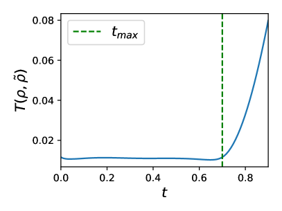
Figure 3: (EXP1) Learning the evolution of a noisy two level system: the mean trace distance $T(\rho(t),\tilde{\rho}(t))=\frac{1}{N_{\mathrm{P}}}\sum_{\beta}D(\rho_{\beta}(t),\tilde{\rho}_{\beta}(t))$ between true states $\rho_{\beta}(t_{j})$ and predicted states $\tilde{\rho}_{\beta}(t_{j})$ as a function of time. The time $t_{max}$ is the maximum time used during training. All the experiments run with the following parameters $\omega=1$ for Eq. 14 and $\lambda=2$, $\gamma_{0}=0.5$ for Eq. 15, and a discretization interval of $\Delta t=0.01$. The simulations run over $3000$ training examples and predictions were tested over $1000$ test examples. All the evolutions run for a time of $t_{max}=0.7$.

We use the above model to obtain training data for the RNN architecture shown in Fig. 2(b). Each training sequence $\rho_{\alpha}(t_{j})$, for $\alpha=1,\dots,N_{\mathrm{I}}$, has been obtained by first choosing a random initial state $\rho_{\alpha}(0)$ and then solving the master equation Eq. (14) to get the states $\rho_{\alpha}(t_{j})$ at subsequent times, up to a maximal time $t_{max}$. These data sequences were then used to train a GRU neural network, by minimising the cost function (11). After training, we test the accuracy of the neural network by generating a new sequence of states $\rho_{\beta}(t_{j})$, and the RNN prediction $\tilde{\rho}_{\beta}(t_{j})$, for $\beta=1,\dots,N_{\mathrm{P}}$. As before, $\rho_{\beta}(t_{j})$ is obtained by selecting a random initial state $\rho_{\beta}(0)$ and solving Eq. (14), possibly for longer times than $t_{max}$. On the other hand, the predicted evolution $\tilde{\rho}_{\beta}(t_{j})$ is obtained by feeding the initial state $\rho_{\beta}(0)$ to the RNN to get the entire temporal sequence. The two evolutions are compared with the trace distance $D(\rho,\tilde{\rho})=\frac{1}{2}\Tr|\rho-\tilde{\rho}|$. In particular, we study the average trace distance $T(\rho(t),\tilde{\rho}(t))=\frac{1}{N_{\mathrm{P}}}\sum_{\beta}D(\rho_{\beta}(t),\tilde{\rho}_{\beta}(t))$ as a function of time.

In Fig. 3 we show a numerical solution of this numerical experiment (EXP1), where we can see that, once trained, the RNN is able to predict the evolution of a known starting state, up to the maximal training time $t_{max}$. On the other hand, and as expected, the accuracy of the RNN prediction rapidly deteriorates for $t>t_{max}$.

IV.2 Learning the master equation: a simple case

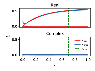
Figure 4: (EXP2) Learning the Lindblad operator describing the Markovian evolution of a two level system: the learned and known entries of $\frac{1}{\alpha}\sum_{\alpha}L^{\mu\equiv 1}$ are compared for the Markovian evolution of a two-level system. We plot the time evolution of every entry of the matrix. Real and complex entries are plotted separately. All the experiments run with the following parameters $\omega=1$ for Eq. (14) and $\lambda=2$, $\gamma_{0}=0.5$ for Eq. (15), and a discretization interval of $\Delta t=0.01$. The simulations run over $1500$ training examples and predictions were tested over $2500$ test examples. All the evolutions run for a time of $t_{max}=0.7$. The Frobenius norm squared was used as distance between the matrices.

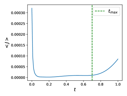
Figure 5: (EXP2) Average cost function value (13) for different times. The parameters are the same of Fig. (4).

In Fig. 4 we show the solution of a second numerical experiment (EXP2) obtained with the same training set of the first experiment (EXP1), discussed in Fig. 3. While EXP1 uses a RNN to model the entire quantum evolution, EXP2 uses the RNN to define a QRN master equation, following Sec. III.3. Training is then performed by minimising the QRN cost function (13), where for simplicity we assume a first-order Runge-Kutta integrator ($n=1$) and a single recurrent Lindblad operator ($\mu\equiv 1$). In EXP2 we have chosen a Markovian regime so that the entire evolution can be modeled via a GKSL master equation (1). In this regime, the RNN Lindblad operators can be approximated as a simple time-dependent function, so the minimization of the cost function (13) is equivalent to learning standard Lindblad operators. In Fig. 4 we compare the predicted recurrent Lindblad operators $L_{\mu}$ as a function of time, with respect to the real ones defined in Eq. (14). In the system under study all entries of the Lindblad operators are zero (hence the flat lines in the figure) apart from one value. As we can see, the prediction is remarkably accurate at all times, even beyond the training time $t>t_{max}$. The error in the prediction is shown in Fig. 5, by plotting the cost function (13) for different times. EXP2 shows that the RNN was able to learn the evolution of the Lindblad operator $L_{t}$ for $t=0.1$ to $t_{max}=0.7$. In addition, the RNN was able to predict $L_{t}$ for $t>t_{max}$ which was the last time step used during training.

IV.3 Learning the master equation: non-Markovian case

In this section we focus on the non-Markovian regime, where there are non-trivial memory effects that the RNN has to learn and reproduce. As in Sec. IV.1, we consider state sequences generated numerically by solving a master equation. However, unlike our previous treatment, here we consider a more complicated non-Markovian model of the environment, which includes back-scattering effects. Back-scattering can refer, for instance, to a photon emitted to the environment that comes back at later times. As such, the information transferred to the environment is not completely lost. To model these non-Markovian effects we consider two qubits evolving with the following master equation

$$\frac{\partial}{\partial t} \rho_{12}(t)=-i[H_{12},\rho_{12}(t)]+$$ (16)

$$+\sum_{i=1}^{2}\gamma_{i}(t)\left(\sigma^{-}_{i}\rho_{12}(t)\sigma^{+}_{i}-\frac{1}{2}\left\{\sigma^{+}_{i}\sigma^{-}_{i},\rho_{12}(t)\right\}\right),$$

where $\gamma_{i}(t)$ has the same functional form of Eq. (15) (but we add a superscript $(i)$ to the parameters $\gamma^{(i)}_{0}$ and $\lambda^{(i)}$ that refers to qubit index) and the two-qubit Hamiltonian is

$$H_{12}=\omega\,\sigma_{z}\otimes I+c_{1}\,\sigma_{x}\otimes\sigma_{x}+c_{2}\,\sigma_{y}\otimes\sigma_{y}+c_{3}\,\sigma_{z}\otimes\sigma_{z},$$ (17)

where $c_{1}=0.3242$, $c_{2}=0.6723$, and $c_{3}=0.1353$. We numerically solve Eq. (16) to get the data sequence $\rho^{\alpha}_{12}(t_{j})$, where $\alpha=1,\dots,N_{\mathrm{I}}$ indexes the different solutions obtained with different initial states. From these two qubit solutions we define then the state sequences as $\rho_{\alpha}(t_{j})=\Tr_{2}[\rho^{\alpha}_{12}(t)]$. In other terms, qubit 1 is the principal system, while qubit 2 is an ancillary system. Because of the coherent interaction $H_{12}$ between qubit 1 and qubit 2, with this approach we can mimic the back-action of the environment onto the system.

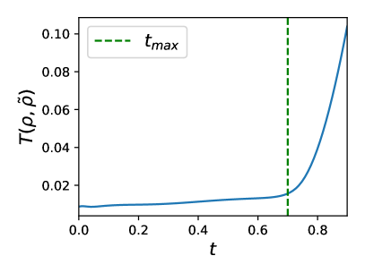
Figure 6: (EXP3) Learning the evolution of a noisy two level non-Markovian system: the mean trace distance $T(\rho(t),\tilde{\rho}(t))=\frac{1}{N_{\mathrm{P}}}\sum_{\beta}D(\rho_{\beta}(t),\tilde{\rho}_{\beta}(t))$ between true states $\rho_{\beta}(t_{j})$ and prediction states $\tilde{\rho}_{\beta}(t_{j})$ as a function of time. The time $t_{max}$ is the maximum time used during training. The experiments run with the following parameters $\lambda^{(1)}=2$, $\gamma^{(1)}_{0}=0.5$ and $\lambda^{(2)}=1$, $\gamma^{(2)}_{0}=0.2$ for Eq. (16), $\omega=1$ for Eq. (17), and a discretization interval of $\Delta t=0.01$. The simulations run over $3000$ training examples and predictions were tested over $1000$ test examples. All the evolutions run for a time of $t_{max}=0.7$.

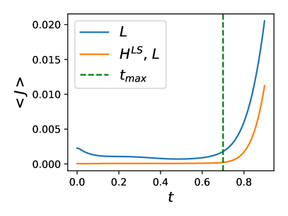
Figure 7: (EXP4) Learning a non-Markovian memory kernel: average value of the cost function $\langle J\rangle$ on unseen examples as a function of time for a learned memory kernel with only the Lindblad Operator $L_{{\leq}t}^{\mu}$ and with both the Lindblad Operator and the Lamb-shift Hamiltonian $H^{LS}_{{\leq}t}$. The parameters are the same of Fig. 6. The Frobenius norm squared was used as distance between the matrices.

We divide our numerical results into different experiments. In EXP3, shown in Fig. 6, we train a RNN to fully reproduce the entire quantum evolution, following the discussion of Sec. III.2. We see that in spite of non-Markovian effects, the resulting error is comparable to that of the Markovian case (EXP1) shown in Fig. 3.

In Fig. 7 we use the same training data of EXP3 to run a new experiment (EXP4) where we train a QRN master equation, by minimising the cost function (13). We consider two cases: in the first one the RNN outputs a single recurrent Lindblad operator $L^{\mu\equiv 1}$. In the second one, the RNN outputs both model both a recurrent Lindblad operator $L^{\mu\equiv 1}$, and the renormalized Hamiltonian, namely the Lamb-shift term $H^{LS}$. We note that, with a single recurrent Lindblad operator, the error is slightly larger than that of the Markovian case, shown in Fig. 4. However, the resulting error is very low when we include also the correction Hamiltonian $H^{LS}$. Comparing Fig. 7 with the Markovian case, Fig. 4, one can see that the error grows faster in the non-Markovian regime after the training time $t_{\rm max}$. Overall, in Fig. 7 we see that the RNN which learned both the recurrent Lindblad operator and the Lamb-shift Hamiltonian performed best, and was better able to predict the memory kernel at times greater than those seen during training.

Figure 8: (EXP5) Learning a non-Markovian master equation with different $\omega$ values: average value of the cost function $\langle J\rangle$ on unseen examples as a function of time for a learned memory kernel with both the Lindblad operator $L_{{\leq}t}^{\mu}$ where $\mu=2$ and the Lamb-shift Hamiltonian $H^{LS}_{{\leq}t}$. $t_{max}$ specifies the maximum time in the range of times used for training. All the experiments run with the following parameters $\lambda^{(1)}=2$, $\gamma^{(1)}_{0}=0.5$ and $\lambda^{(2)}=1$, $\gamma^{(2)}_{0}=0.2$ for Eq. (16), $\omega$ uniformly sampled in the interval $[0.5,1.5]$ for Eq. (17), and a discretization interval of $\Delta t=0.01$. The simulations run over $3000$ training examples and predictions were tested over $1000$ test examples. All the evolutions run for a time of $t_{max}=0.7$. The Frobenius norm squared was used as distance between the matrices.

Finally, in Fig. 8 we run a different numerical experiment (EXP5). In EXP5 the training set is composed by data sequences where the qubit frequency $\omega$ in Eq. (17) is not fixed, but rather uniformly sampled from 0.5 to 1.5. The sampled frequency is used as an extra input to the RNN. This corresponds to the experimentally relevant case where the qubit frequency can be externally tuned to a known value. Uncertainty about this frequency can be estimated from the correction Hamiltonian $H^{LS}$, which is learned from the data. In Fig. 8 we see that the error in EXP5 is remarkably low. Based on the success of this numerical experiment, we propose the following general strategy to introduce prior knowledge about the system. We can define a RNN where the known properties of the system, e.g. its Hamiltonian, are added as an extra input. Training is performed using datasets of quantum state sequences and their respective Hamiltonian, where the latter is sampled from the space of experimentally relevant Hamiltonians. The remarkable accuracy shown Fig. 8 suggests that this procedure forces the RNNs to better explore the manifold of quantum state sequences, to produce a more accurate and robust prediction.

V Conclusions and Perspectives

We have studied quantum state evolution using RNNs. We have shown that even when the system is interacting with a complicated surrounding environment, RNNs offer an accurate and robust tool for modeling and reconstructing the quantum evolution, both in the Markovian and non-Markovian regime, and even when there are back-scattering effects from the environment.

We have introduced two approaches for modelling open quantum systems with RNNs. In the first one, a deep RNN is trained to learn the entire quantum evolution, namely to reproduce the time sequence $\rho(t_{j})$ given an initial state $\rho(0)$. In the second approach, we use a deep RNN to define a non-Markovian master equation where the memory kernel takes a convenient mathematical form, namely that of the GKSL equation. In our master equation the non-Markovian memory effects are taken into account by the structure of the RNN cells. The observed success of our approaches stems from the ability of RNNs to learn temporal sequences, where the future depends on the entire past. Our RNN-based master equation can be used as a convenient mathematical framework to write non-Markovian memory kernels without resorting to perturbative treatments, and to learn their unknown parameters directly from the data.

Many extensions of our work are possible. Many-body systems with exponentially large Hilbert spaces could be considered by using RNNs which output a compressed representation of the state, such as tensor networks Cui et al. (2015); Vidal (2008), restricted Boltzmann machines Torlai et al. (2018) or variational autoencoders Rocchetto et al. (2018). The predictions after the training time can be improved by considering higher order Runge Kutta integrators and by modifying the structure of the RNN cell to have a fixed point in the infinite time limit, as expected from physical principles. Although RNNs proved to be a powerful tool for modelling open quantum systems, the machine learning literature offers a number of other methods, such as Kalman Filters or models with Gaussian Process transitions, that appear particularly promising. For example, Gaussian Process State Space Models Frigola et al. (2014) allow one to model prior information on the system and return Bayesian estimates of the uncertainties. Both these features are desirable in a quantum context: prior knowledge on the system, such as the form of the noise-free Hamiltonian, may be used to further reduce the complexity of the model, while approximate values for the uncertainties might enable better control of experimental inaccuracies. It would be interesting to define quantum master equations based on these tools and to check their performances against our QRN master equation.

Finally, in more physical terms, it would be interesting to study what happens when partial information about the system is available. An experimentally relevant case is when the initial state $\rho(0)$ is known, but one has access to a limited set of expectation values $\langle{A_{k}}\rangle_{\rho(t_{j})}$, where the observables $A_{k}$ are not enough to tomographically reconstruct the states $\rho(t_{j})$. This possibility may be considered, using our framework, by introducing a cost function between expectation values, rather than between density operators. A further challenge is then to model the disturbance of the measurement onto the system, namely the wave function collapse. This can be done using the process tensor formalism Pollock et al. (2018), which provides an avenue for generalising our approach in the presence of feedback. It would be interesting to study the performance of RNNs to model these experimentally relevant quantum evolutions.

Appendix A Gated Recurrent Unit

The GRU state $s_{t}$ is a linear interpolation of the previous state $s_{t-1}$ and a candidate state $\tilde{s}_{t}$. The candidate state is a function of the cell input $x_{t}$ and the previous state given by:

$$\begin{split}z_{t}&=\sigma(W_{z}x_{t}+U_{z}s_{t-1}+b_{z})~{},\\ r_{t}&=\sigma(W_{r}x_{t}+U_{r}s_{t-1}+b_{r})~{},\\ \tilde{s}_{t}&=\tanh(Wx_{t}+U(r_{t}\circ s_{t-1})+b)~{},\\ s_{t}&=(1-z_{t})\circ s_{t-1}+z_{t}\circ\tilde{s}_{t}~{},\end{split}$$ (18)

where $\circ$ denotes the entry-wise (Hadamard) product, $\sigma$ denotes the sigmoid function, $x_{t}$ is the input to the cell and $W$, $U$ and $b$ are trainable parameters, which do not explicitly depend on $t$. GRU cells can be stacked to form a deep GRU network. The input $x^{j}_{t}$ for a depth $j$ cell at time $t$ is the state from the cell in the previous layer $s^{j-1}_{t}$.

The GRU state $s_{t}$ can be thought of as a mixture of the previous state $s_{t-1}$ and the candidate state $\tilde{s}_{t}$. The weighting of the mixture is controlled by $z_{t}$ which is known as the update gate. We can see that if the entries of $z_{t}$ are zero then the candidate state is ignored and the previous state becomes the new state.

The candidate state $\tilde{s}_{t}$ is a function of the previous state $s_{t-1}$ and the current input $x_{t}$. The relative contribution of the previous state to the candidate state is controlled by $r_{t}$ which is known as the reset gate.

A more detailed discussion of GRU cells can be found in Ref. Cho et al. (2014).

Note that the output of the network is a real vector. In order to encode complex matrices into the RNN we use the following procedure. Assume that we want to encode a matrix $M\in\mathbb{C}^{m\times m}$. $M$ can be decomposed into a real and imaginary part $M=M_{\mathrm{Re}}+iM_{\mathrm{Im}}$. We require the output of the RNN to be a vector $o\in\mathbb{R}^{2m^{2}}$ such that the first $m^{2}$ elements encode in row-major order the entries of $M_{\mathrm{Re}}$ and the second $m^{2}$ elements encode in row-major order the entries of $M_{\mathrm{Im}}$.

All GRU networks used in this work consisted of $2$ GRU layers with output dimension = $40$, followed by $1$ fully connected layer. The Adam optimizer was used for training with initial learning rate $0.01$ Kingma and Ba (2014) and batches of $32$ examples. Training was stopped after each example was seen $60$ times. In EXP2 the fully connected weights were regularized using weight decay Krogh and Hertz (1992), with the L2 penalty factor set to 0.001. The networks were implemented using the Keras $2.2.0$ and Tensorflow $1.8$ frameworks Chollet et al. (2015); Abadi et al. (2016). Network weights were initialized using the Keras defaults.

References

- Bishop (2006) C. M. Bishop, Pattern Recognition and Machine Learning (Information Science and Statistics) (Springer-Verlag, Berlin, Heidelberg, 2006).
- LeCun et al. (2015) Y. LeCun, Y. Bengio, and G. Hinton, Nature 521, 436 (2015).
- Pathak et al. (2018) J. Pathak, B. Hunt, M. Girvan, Z. Lu, and E. Ott, Physical Review Letters 120, 024102 (2018).
- Komiske et al. (2017) P. T. Komiske, E. M. Metodiev, and M. D. Schwartz, Journal of High Energy Physics 2017, 110 (2017).
- Schuld et al. (2015) M. Schuld, I. Sinayskiy, and F. Petruccione, Contemporary Physics 56, 172 (2015).
- Biamonte et al. (2017) J. Biamonte, P. Wittek, N. Pancotti, P. Rebentrost, N. Wiebe, and S. Lloyd, Nature 549, 195 (2017).
- Ciliberto et al. (2018) C. Ciliberto, M. Herbster, A. D. Ialongo, M. Pontil, A. Rocchetto, S. Severini, and L. Wossnig, Proc. R. Soc. A 474, 20170551 (2018).
- Dunjko and Briegel (2018) V. Dunjko and H. J. Briegel, Reports on Progress in Physics 81, 074001 (2018).
- Carleo and Troyer (2017) G. Carleo and M. Troyer, Science 355, 602 (2017).
- Torlai et al. (2018) G. Torlai, G. Mazzola, J. Carrasquilla, M. Troyer, R. Melko, and G. Carleo, Nature Physics , 1 (2018).
- Yu et al. (2018) S. Yu, F. Albarran-Arriagada, J. Retamal, Y.-T. Wang, W. Liu, Z.-J. Ke, Y. Meng, Z.-P. Li, J.-S. Tang, E. Solano, et al., arXiv preprint arXiv:1808.09241 (2018).
- van Nieuwenburg et al. (2017) E. P. van Nieuwenburg, Y.-H. Liu, and S. D. Huber, Nature Physics 13, 435 (2017).
- Gray et al. (2018) J. Gray, L. Banchi, A. Bayat, and S. Bose, Physical review letters 121, 150503 (2018).
- Carrasquilla and Melko (2017) J. Carrasquilla and R. G. Melko, Nature Physics 13, 431 (2017).
- Mehta and Schwab (2014) P. Mehta and D. J. Schwab, arXiv preprint arXiv:1410.3831 (2014).
- Levine et al. (2017) Y. Levine, D. Yakira, N. Cohen, and A. Shashua, CoRR, abs/1704.01552 (2017).
- Levine et al. (2018) Y. Levine, O. Sharir, N. Cohen, and A. Shashua, arXiv preprint arXiv:1803.09780 (2018).
- Chen et al. (2018) J. Chen, S. Cheng, H. Xie, L. Wang, and T. Xiang, Physical Review B 97, 085104 (2018).
- Rocchetto et al. (2018) A. Rocchetto, E. Grant, S. Strelchuk, G. Carleo, and S. Severini, npj Quantum Information 4, 28 (2018).
- Banchi et al. (2016) L. Banchi, N. Pancotti, and S. Bose, npj Quantum Information 2, 16019 (2016).
- Innocenti et al. (2018) L. Innocenti, L. Banchi, A. Ferraro, S. Bose, and M. Paternostro, arXiv preprint arXiv:1803.07119 (2018).
- Eloie et al. (2018) L. Eloie, L. Banchi, and S. Bose, Phys. Rev. A 97, 062321 (2018).
- Las Heras et al. (2016) U. Las Heras, U. Alvarez-Rodriguez, E. Solano, and M. Sanz, Physical Review Letters 116, 230504 (2016).
- Zahedinejad et al. (2016) E. Zahedinejad, J. Ghosh, and B. C. Sanders, Physical Review Applied 6, 054005 (2016).
- Verdon et al. (2018) G. Verdon, J. Pye, and M. Broughton, arXiv preprint arXiv:1806.09729 (2018).
- Grant et al. (2018) E. Grant, M. Benedetti, S. Cao, A. Hallam, J. Lockhart, V. Stojevic, A. G. Green, and S. Severini, arXiv preprint arXiv:1804.03680 (2018).
- Melnikov et al. (2018) A. A. Melnikov, H. P. Nautrup, M. Krenn, V. Dunjko, M. Tiersch, A. Zeilinger, and H. J. Briegel, Proceedings of the National Academy of Sciences , 201714936 (2018).
- Huggins et al. (2018) W. Huggins, P. Patel, K. B. Whaley, and E. M. Stoudenmire, arXiv preprint arXiv:1803.11537 (2018).
- Benedetti et al. (2018) M. Benedetti, E. Grant, L. Wossnig, and S. Severini, arXiv preprint arXiv:1806.00463 (2018).
- Bukov et al. (2018) M. Bukov, A. G. Day, D. Sels, P. Weinberg, A. Polkovnikov, and P. Mehta, Physical Review X 8, 031086 (2018).
- Niu et al. (2018) M. Y. Niu, S. Boixo, V. Smelyanskiy, and H. Neven, arXiv preprint arXiv:1803.01857 (2018).
- Breuer and Petruccione (2002) H.-P. Breuer and F. Petruccione, The theory of open quantum systems (Oxford University Press on Demand, 2002).
- Rivas and Huelga (2012) A. Rivas and S. F. Huelga, Open Quantum Systems (Springer, 2012).
- Ishizaki and Fleming (2009) A. Ishizaki and G. R. Fleming, The Journal of chemical physics 130, 234111 (2009).
- Pollock et al. (2018) F. A. Pollock, C. Rodríguez-Rosario, T. Frauenheim, M. Paternostro, and K. Modi, Physical Review A 97, 012127 (2018).
- August and Ni (2017) M. August and X. Ni, Physical Review A 95, 012335 (2017).
- Ostaszewski et al. (2018) M. Ostaszewski, J. Miszczak, P. Sadowski, and L. Banchi, arXiv preprint arXiv:1803.05193 (2018).
- Gorini et al. (1976) V. Gorini, A. Kossakowski, and E. C. G. Sudarshan, Journal of Mathematical Physics 17, 821 (1976).
- Lindblad (1976) G. Lindblad, Communications in Mathematical Physics 48, 119 (1976).
- Ciccarello et al. (2013) F. Ciccarello, G. Palma, and V. Giovannetti, Physical Review A 87, 040103 (2013).
- Ziman et al. (2002) M. Ziman, P. Štelmachovič, V. Bužek, M. Hillery, V. Scarani, and N. Gisin, Physical Review A 65, 042105 (2002).
- Giovannetti and Palma (2012) V. Giovannetti and G. M. Palma, Physical Review Letters 108, 040401 (2012).
- Rybár et al. (2012) T. Rybár, S. N. Filippov, M. Ziman, and V. Bužek, Journal of Physics B: Atomic, Molecular and Optical Physics 45, 154006 (2012).
- McCloskey and Paternostro (2014) R. McCloskey and M. Paternostro, Physical Review A 89, 052120 (2014).
- Ciccarello (2017) F. Ciccarello, Quantum Measurements and Quantum Metrology 4, 53 (2017).
- Campbell et al. (2018) S. Campbell, F. Ciccarello, G. M. Palma, and B. Vacchini, arXiv preprint arXiv:1805.09626 (2018).
- Binder et al. (2018) F. C. Binder, J. Thompson, and M. Gu, Physical Review Letters 120, 240502 (2018).
- Cerrillo and Cao (2014) J. Cerrillo and J. Cao, Physical Review Letters 112, 110401 (2014).
- Pollock and Modi (2017) F. A. Pollock and K. Modi, arXiv preprint arXiv:1704.06204 (2017).
- Howard et al. (2006) M. Howard, J. Twamley, C. Wittmann, T. Gaebel, F. Jelezko, and J. Wrachtrup, New Journal of Physics 8, 33 (2006).
- Yuen-Zhou et al. (2011) J. Yuen-Zhou, J. J. Krich, M. Mohseni, and A. Aspuru-Guzik, Proceedings of the National Academy of Sciences 108, 17615 (2011).
- Bellomo et al. (2010) B. Bellomo, A. De Pasquale, G. Gualdi, and U. Marzolino, Journal of Physics A: Mathematical and Theoretical 43, 395303 (2010).
- Wiebe et al. (2014) N. Wiebe, C. Granade, C. Ferrie, and D. G. Cory, Physical review letters 112, 190501 (2014).
- Breuer et al. (2016) H.-P. Breuer, E.-M. Laine, J. Piilo, and B. Vacchini, Reviews of Modern Physics 88, 021002 (2016).
- Banchi et al. (2013) L. Banchi, G. Costagliola, A. Ishizaki, and P. Giorda, The Journal of chemical physics 138, 05B609_1 (2013).
- Mukamel (1999) S. Mukamel, Principles of nonlinear optical spectroscopy, 6 (Oxford University Press on Demand, 1999).
- Zhang et al. (2012) W.-M. Zhang, P.-Y. Lo, H.-N. Xiong, M. W.-Y. Tu, and F. Nori, Physical Review Letters 109, 170402 (2012).
- Jang and Silbey (2003) S. Jang and R. J. Silbey, The Journal of chemical physics 118, 9312 (2003).
- Chruściński and Kossakowski (2010) D. Chruściński and A. Kossakowski, Physical Review Letters 104, 070406 (2010).
- Schmidhuber (2015) J. Schmidhuber, Neural networks 61, 85 (2015).
- Cho et al. (2014) K. Cho, B. Van Merriënboer, C. Gulcehre, D. Bahdanau, F. Bougares, H. Schwenk, and Y. Bengio, arXiv preprint arXiv:1406.1078 (2014).
- Hochreiter and Schmidhuber (1997) S. Hochreiter and J. Schmidhuber, Neural computation 9, 1735 (1997).
- Chung et al. (2014) J. Chung, C. Gulcehre, K. Cho, and Y. Bengio, arXiv preprint arXiv:1412.3555 (2014).
- Lipton et al. (2015) Z. C. Lipton, J. Berkowitz, and C. Elkan, arXiv preprint arXiv:1506.00019 (2015).
- Vacchini et al. (2011) B. Vacchini, A. Smirne, E.-M. Laine, J. Piilo, and H.-P. Breuer, New Journal of Physics 13, 093004 (2011).
- Schmidt and Lipson (2009) M. Schmidt and H. Lipson, science 324, 81 (2009).
- Süli and Mayers (2003) E. Süli and D. Mayers, An Introduction to Numerical Analysis (Cambridge University Press, 2003).
- Breuer et al. (1999) H.-P. Breuer, B. Kappler, and F. Petruccione, Physical Review A 59, 1633 (1999).
- Chruściński and Maniscalco (2014) D. Chruściński and S. Maniscalco, Physical Review Letters 112, 120404 (2014).
- Bylicka et al. (2014) B. Bylicka, D. Chruściński, and S. Maniscalco, Scientific reports 4, 5720 (2014).
- Iles-Smith et al. (2016) J. Iles-Smith, A. G. Dijkstra, N. Lambert, and A. Nazir, The Journal of chemical physics 144, 044110 (2016).
- Cui et al. (2015) J. Cui, J. I. Cirac, and M. C. Banuls, Physical Review Letters 114, 220601 (2015).
- Vidal (2008) G. Vidal, Physical Review Letters 101, 110501 (2008).
- Frigola et al. (2014) R. Frigola, Y. Chen, and C. E. Rasmussen, in Advances in Neural Information Processing Systems (2014) pp. 3680–3688.
- Kingma and Ba (2014) D. P. Kingma and J. Ba, arXiv preprint arXiv:1412.6980 (2014).
- Krogh and Hertz (1992) A. Krogh and J. A. Hertz, in Advances in neural information processing systems (1992) pp. 950–957.
- Chollet et al. (2015) F. Chollet et al., “Keras,” https://keras.io (2015).
- Abadi et al. (2016) M. Abadi, P. Barham, J. Chen, Z. Chen, A. Davis, J. Dean, M. Devin, S. Ghemawat, G. Irving, M. Isard, et al., in OSDI, Vol. 16 (2016) pp. 265–283.