Higgs Physics: It ain’t over till it’s over
Abstract
We review the theoretical underpinning of the Higgs mechanism of electroweak symmetry breaking and the experimental status of Higgs measurements from a pedagogical perspective. The possibilities and motivations for new physics in the symmetry breaking sector are discussed along with current measurements. A focus is on the implications of measurements in the Higgs sector for theoretical insights into extensions of the Standard Model. We also discuss of future prospects for Higgs physics and new analysis techniques.
feynman
Introduction
The Higgs discovery in 2012 can be considered the most unusual, yet arguably most important discovery in the history of particle physics. “Most unusual” because it was entirely expected, which stands in stark contrast to other paradigm-shifting discoveries such as during the November revolution in 1974. “Most important” as it marks the ultimate test of perturbative quantum field theory as a theoretical framework, validating spontaneous symmetry breaking as the only remaining realization of gauge symmetry after linear realizations such as QCD and QED had been tested with tremendous success.
The Higgs discovery completed the Standard Model (SM) of particle physics, which after subsequent measurements not only in Higgs related channels at the Large Hadron Collider (LHC) stands firmly as Occam’s Razor of fundamental particle interactions. The Standard Model is relatively simple quantum field theory, the minimal symmetry and particle content required by measurements seems to be perfectly sufficient to explain a range of phenomena over a many orders of magnitude. Yet we know that the Standard Model cannot be the final answer to fundamental interactions in nature. Typically one mentions gravity as the prime example of a fundamental force that is not included in the Standard Model and it is fair to say that the basics of its fundamental quantum mechanical nature are yet to understood. But there are phenomena more closely related to our usual thinking of particle physics that are not addressed in the Standard Model, such as dark matter, which could well fit into our well-established framework of perturbative quantum field theory. Besides this obvious negligence of phenomenological facts, there theoretical arguments against the Standard Model, which have served as motivations to construct various avenues of physics beyond the Standard Model. One of the most famous ones is probably the hierarchy problem that states that fundamental scalars imply relevant mass parameters from a renormalization group point of view. As “traditional” gauge symmetry principles are not sufficient to mend the instability of the Higgs mass against radiative corrections in the presence of large new physics scales, qualitatively different extensions of the Standard Model need to be formulated. These include various scenarios of Supersymmetry and strong interactions, where the latter seeks to explain the electroweak scale as a dimensional transmutation effect similar to QCD.
Irrespective of their theoretical appeal or our prejudice as theoretical physicists, we have effectively entered a era of particle physics that is marked by its return to a measurement-driven character. Although this seems unusual in the context of particle physics where model-building has crucially influenced experimental measurement and design strategies over the past four decades, it is a common denominator of all physical sciences. While we still look for concrete UV scenarios at the LHC, more model-independent approaches have gained attention and efforts in creating adapted (data-driven) analysis approaches have been intensified.
It is the purpose of this review to provide a pedagogical snapshot of Higgs physics six years into the LHC’s Higgs phenomenology program. We review production and decay processes as well as their perturbative history that led to the Higgs boson discovery in 2012. We discuss well-motivated extensions beyond the Standard Model, how they have been searched for at the LHC, as well as their current phenomenological status. We also discuss how these measurements affect the current discussion on the direction that the field might take in the future after the LHC.
A Theoretical basis
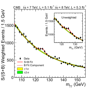
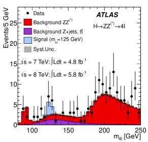
Higgs physics is one of the few instances in fundamental physics where a theoretical idea or concept was discovered experimentally exactly the way it was predicted Higgs (1964a, b); Englert and Brout (1964); Guralnik et al. (1964); Kibble (1967); Higgs (1966) 111If you feel strongly that we are missing a reference, please send a friendly email to niceguy@englert.com, and we will include it. If you just want us to cite one more of your papers, please email to devnull@ihateyoutilman.com.. In that sense, the discovery of the Higgs boson in 2012 marks the coming of age of one of the largest and longest-lasting projects in fundamental physics. The Higgs boson was discovered in 2012 Chatrchyan et al. (2012); Aad et al. (2012) through the predicted resonant decays to and as seen in Fig. 1. This discovery is now established and there can be no doubt that a particle with properties close to those predicted decades ago has been discovered with the mass is measured rather accurately Aad et al. (2015a) to be
| (A.1) |
In the first part of this review we discuss the basic structure of the Higgs mechanism in the Standard Model, discuss extended models and the formalism of effective field theory as a preferred theory framework for LHC studies. Next, we comment on the current experimental status, organized by LHC signatures. We touch on possible future developments in Higgs physics at the LHC, ILC, and future high energy hadron machines. Finally, we close with a discussion of new analysis techniques for Higgs physics.
1 Historical introduction
In some sense, Higgs physics started with Fermi’s theory in 1934 Fermi (1934). While this theory offers a valid description of beta decay, muon decay, and many other low-energy phenomena, it turns out to have a fundamental problem: the interaction strength of the four-fermion interaction has an inverse mass dimension. This leads to structural problems when we want to unify it with the proto-typical fundamental quantum field theory of quantum electrodynamics (QED). The main difference between these two theories is that the photon is a massless vector boson, while the agent of the weak interaction has a mass that can be linked to the inverse Fermi coupling. This mass shields the interactions at large distances and transforms a Coulomb-like potential into a Yukawa potential. The fundamental theoretical question therefore is: how can we break the gauge symmetry describing the weak interaction such that at high energies it can be unified with QED while remaining compatible with Fermi’s theory at low energies?
The Brout-Englert-Higgs trick Anderson (1963); Englert and Brout (1964); Higgs (1964a, b), or spontaneous symmetry breaking, is to not break the weak gauge symmetry explicitly or at the level of the Lagrangian. Instead, it realizes it non-linearly through the presence of an additional scalar field Fujikawa et al. (1972); Becchi et al. (1974, 1975, 1976); Tyutin (1975) (see also ’t Hooft (1994)). In this way electroweak symmetry can be compatible with a large non-vanishing background expectation value of the scalar field. A phenomenological consequence of this approach that is commonly referred to as the Higgs mechanism is the appearance of longitudinal degrees of freedom for the involved gauge bosons, which behave like derivatives of scalar fields in the deep ultraviolet regime of momenta. The ingenious idea of realizing electroweak symmetry this way therefore effectively restores the standard power counting arguments of perturbative quantum field theory Weinberg (1960) that are at the core of ultraviolet renormalizability ’t Hooft and Veltman (1972), which again is the theoretical underpinning of the theoretical progress that was necessary to finally discover the Higgs boson. Strictly speaking, spontaneous symmetry breaking is a slight abuse of language as the gauge symmetry is not broken and the vacuum is invariant under local gauge transformations. The semi-classical treatment of non-linearly realized local symmetries and spontaneously broken global symmetries at the level of Lagrangians is similar, while the consequences for the quantum dynamics are vastly different. Given the semi-classical analogy, we can therefore pretend that we are dealing with identical approaches while implicitly relying on the fact that the quantum theory will make allowances for our ignorance.
The fundamental problem of breaking the weak symmetry is not introducing an appropriate breaking term in the Lagrangian and justifying its existence. The problem is that a massless gauge boson has two degrees of freedom, while a massive gauge boson requires three degrees of freedom, and the third or longitudinal degree of freedom has to come from somewhere. The solution is linked to Goldstone’s theorem Goldstone (1961), which in the particular case of a weak symmetry naively implies that three broken generators give rise to three massless degrees of freedom in the low energy spectrum of the theory. When we gauge the symmetry, these degrees of freedom combine with the two massless degrees of freedom of a massless gauge boson to form massive -bosons. In addition, a quantum description predicts excitations around the vacuum expectation value, the new Higgs boson. In general, the Goldstone modes and the Higgs mode will therefore not form a common multiplet under a given symmetry. They define an effective field theory with a non-linear realization of the weak symmetry, as described in Sec. 7.
In the ultraviolet extension of Fermi’s theory Glashow (1961); Salam and Ward (1964); Weinberg (1967a) the three Goldstone modes are part of an doublet. Such a complex doublet has four degrees of freedom, and the fourth direction is identified with the vacuum expectation value (VEV) and the additional scalar field, Higgs (1964a),
| (A.2) |
The building block is invariant under all symmetries of the Standard Model. The Higgs VEV can be traced to a non-trivial minimum of the potential
| (A.3) |
with . If we limit ourself to this potential, we can relate the two parameters and to two (pseudo)observables, the Higgs VEV and the physical Higgs boson mass
| (A.4) |
The triple and quartic self-couplings of the physical Higgs bosons are predicted to be
| (A.5) |
allowing for a consistency test of the renormalizable Higgs sector of the Standard Model.
The fact that the Higgs potential in Eq.(A.3) is truncated at dimension four reflects our theoretical bias that a fundamental theory should not feature couplings with inverse mass dimensions. Forgetting this bias for a moment, we can add higher powers of the gauge-invariant building block to the Higgs potential,
| (A.6) |
where we assume for convergence and consistency reasons. The Higgs VEV and mass then become,
| (A.7) |
which breaks the correlations of Eqs. (A.4) and (A.5). Such higher-dimensional terms including the doublet are the basis of a linearly realized effective theory, that will be discussed in detail in Sec. 7. Extended Higgs potentials, which after integrating out heavier additional Higgs states lead to higher-dimensional operators, are at the heart of many of the theoretical constructions discussed in Sec. 5.
2 Weinberg-Salam Model
In the Standard Model, the Higgs mechanism serves two independent purposes. First, it introduces masses for the weak gauge bosons in an, as we know now, renormalizable and perturbative gauge theory. Second, it allows us to write fermion masses for all fermions where the left-handed spinors are part of a weak doublet, while the right-handed spinors are weak singlets. Per se, these two aspects are not related. Moreover, this kind of mass generation does not include the neutrinos, which are missing a light right-handed component in the SM context.
2.1 Gauge sector
The Higgs mechanism of the previous section is embedded in the Weinberg-Salam model of electroweak interactions Weinberg (1967a); Glashow (1961); Goldstone et al. (1962); Salam and Ward (1964). The theory is an gauge theory containing three gauge bosons, , and one gauge boson, . Their kinetic energy terms read
| (A.8) |
where the index is summed over and,
| (A.9) |
The and coupling constants are and , respectively.
The scalar contribution to the Lagrangian is,
| (A.10) |
where is given in Eq.(A.3) and
| (A.11) |
where are the Pauli matrices. This covariant derivative describes the Higgs interactions with the massive gauge bosons, and is the hypercharge of the Higgs boson.
In unitary gauge there are no Goldstone bosons and only the physical Higgs scalar remains in the spectrum after the spontaneous symmetry breaking in the Higgs potential of Eq.(A.3) has occurred. The spontaneous symmetry breaking results in two charged gauge fields, , and two neutral gauge bosons, and .
| (A.12) |
The massless neutral mode is the photon, mediating the electromagnetic interaction. The mixing pattern of Eq.(A.12) defines the weak mixing angle,
| (A.13) |
Since the massless photon must couple with electromagnetic strength, , the coupling constants are related to the weak mixing angle ,
| (A.14) |
The gauge bosons obtain masses from the Higgs mechanism,
| (A.15) |
In a gauge other than unitary gauge we have to account for the Goldstone bosons in the particle spectrum. A complete set of Feynman rules is conveniently given in Ref. Romao and Silva (2012).
2.2 Fermion sector
The and charge assignments of the first generation of fermions are given in Table 1. The quantum numbers of the and generations are identical to those of the first generation and the hypercharge satisfies the relationship, .
| Field | |||
Direct fermion mass terms are forbidden by the assignments of Table 1. The Higgs boson can generate fermion masses through the couplings
| (A.16) |
where is the charge-conjugated Higgs doublet. After the Higgs obtains a VEV, all of the fermions except the neutrinos obtain masses and the Higgs-fermion couplings are proportional to the fermion masses,
| (A.17) |
For the multi-family case, the Yukawa couplings, and , become matrices, where is the number of families. Since the fermion mass matrices and Yukawa matrices are proportional to each other, the interactions of the Higgs boson with the fermion mass eigenstates are flavor diagonal and the Higgs boson does not mediate flavor changing interactions. This is an important prediction of the Standard Model and the discovery of flavor changing Higgs decays would be a clear signal of physics beyond the Standard Model Bjorken and Weinberg (1977); Barr and Zee (1990) .
The numerical value of the Higgs VEV can be extracted from the charged current result for decay, . It is measured very accurately to be . Since the momentum carried by the boson is of order it can be neglected in comparison with and we make the identification,
| (A.18) |
This leaves the Higgs mass as the only free parameter in the scalar potential.
2.3 Custodial symmetry
One of the most important features of the minimalistic Higgs mechanism in the Standard Model is that all of the couplings of the Higgs boson to fermions and gauge bosons are completely determined in terms of the gauge coupling constants, the Higgs mass and fermion masses, and the VEV, . Moreover, at tree level, the different gauge boson masses are related as
| (A.19) |
The relation of the eigenvalues of the mixing matrix are aligned with the characteristic rotation angle of the associated basis transformation . This relation follows from an accidental symmetry of the scalar potential that can be seen by rewriting the Higgs field as a bi-doublet,
| (A.20) |
as transforms identically as (the doublet representation of SU(2) is symplectic). The Higgs potential can now be written as,
| (A.21) |
and features a global symmetry which is broken to a global diagonal symmetry when gets a VEV. This is the custodial symmetry. It is broken by the gauging of hypercharge () and by the mass difference between the top and bottom quarks Degrassi et al. (1991),
| (A.22) |
The leading one-loop corrections to vanish when and . The power dependence on the top mass and the logarithmic dependence on the Higgs mass will be reflected in the sensitivity of electroweak precision measurements to these parameters.
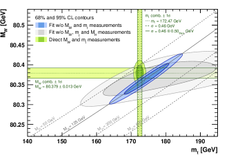
The full set of electroweak data from LEP Schael et al. (2006), the Tevatron and the LHC, including Higgs data, can be used to test the self consistency of the theory, as demonstrated in Fig. 2. The most restrictive data points are the measurements of the coupling and the boson mass. When the experimental values of , , and are omitted, the fit is in good agreement with the directly measured values of the masses. Note that the fit excludes a large ( of GeV) value of and so even before the Higgs boson was discovered, we knew that if there were no new physics contributions to the predictions for electroweak quantities such as , the Higgs boson could not be too heavy.
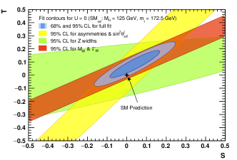
The experimental closeness of to has strong implications for new physics models. Extensions of the Standard Model with modified Higgs sectors are significantly restricted by the requirement of consistency with the electroweak measurements. A simple way to examine whether a theory with an extended Higgs sector is consistent with electroweak experiments is to use the oblique parameters, and Peskin and Takeuchi (1990, 1992); Altarelli and Barbieri (1991). Using the oblique parameters to obtain limits on Beyond the Standard Model physics assumes that the dominant contributions resulting from the expanded theory are to the gauge boson 2-point functions. Current experimental limits on and are shown in Fig. 2, featuring the typical correlation along the diagonal Bardin et al. (2001); Haller et al. (2018); de Blas et al. (2016).
3 Higgs Decays
The Weinberg-Salam model predicts all Higgs production and decay rates, once the Higgs boson mass is known. The main feature is that the Higgs will prefer to decay to the heaviest particles allowed, with longitudinal gauge boson polarizations playing a particular role. As such, it is a testable theory, and non-standard values for Higgs rates would be indications of new physics. This has inspired an immense theoretical effort to obtain predictions for Higgs processes to the highest possible order in perturbation theory, along with resummation of large logarithms. Numerical values including the most up-to-date theoretical calculations have been tabulated by the LHC Higgs cross section working group Dittmaier et al. (2011) (for the most recent update see de Florian et al. (2016a)) and we review the status of the Standard Model predictions here.
Expressions for the SM Higgs decay widths at leading order can be found in Ref. Gunion et al. (2000), and the QCD and electroweak corrected rates, with references to the original literature, are given in Refs. Djouadi (2008); Spira (2017). The NLO corrected decay rates can be found using the public codes Hdecay Djouadi et al. (1998, 2018) and Prophecy4f Bredenstein et al. (2007).
3.1 Fermions
The Higgs couplings to fermions are proportional to the fermion mass and the lowest order width for the Higgs decay to fermions of mass is,
| (A.23) |
where and for charged leptons (quarks), related to their color charge. The leading fermion decay channel is , which receives large QCD corrections. A significant portion of the QCD corrections can be accounted for by expressing the decay width in terms of a running quark mass, evaluated at the scale , indicating that the large effects are triggered by large logarithms. The QCD corrected decay width can be approximated as Drees and Hikasa (1990); Braaten and Leveille (1980),
| (A.24) |
where is defined in the scheme with flavors. The electroweak radiative corrections to amount to the expected few-percent correction Dabelstein and Hollik (1992); Kniehl (1994).
3.2 Weak bosons
The Higgs boson can also decay to weak boson pairs. At tree level, the decays and are possible, if we allow for the gauge bosons to be off-shell. Over most of phase space we can assume that one of the two gauge bosons decays on its mass shell, while the other is pushed into its sizeable Breit-Wigner tails. The decay width for such a decay, , is,
| (A.25) |
where and . The usual Kaellen function is , and the integration boundaries for are given by . The amplitude-squared is,
| (A.26) |
with , , and . Integrating over we find the differential decay rate
| (A.27) |
The result for can be found by making the appropriate redefinitions of the fermion-gauge boson couplings. Performing the integral over the invariant mass of the two fermions and summing over the final state fermions gives us Rizzo (1980); Keung and Marciano (1984),
| (A.28) |
where
| (A.29) |
The NLO QCD and electroweak corrections to the fully off-shell decays, , are implemented in the public code Prophecy4f Bredenstein et al. (2007). Going beyond the total decay rate and instead studying the -distribution is a powerful tool in studying the Lorentz structure of the coupling.
3.3 Gluons
The decay of the Higgs boson to gluons, just like the production process of the Higgs in gluon fusion, only arises through fermion loops in the Standard Model and is sensitive to colored particles that interact with the Higgs Georgi et al. (1978); Ellis et al. (1979); Rizzo (1980),
| (A.30) |
where and the loop function is defined to be,
| (A.31) |
It includes one power of the Yukawa coupling, expressed in terms of the mass, and the re-scaled scalar one-loop three-point function
| (A.32) |
In the limit in which the (bottom) quark mass is much less than the Higgs boson mass the loop function becomes
| (A.33) |
On the other hand, for a heavy top quark, , it approaches a constant,
| (A.34) |
These two limits make it clear that the top quark loop is the dominant contribution. QCD corrections to the decay are known to N3LO Baikov and Chetyrkin (2006). Another theoretical aspect we can read off Eq.(A.34) is that the top contribution to the effective Higgs-gluon coupling does not vanish for large top masses. The reason for this non-decoupling behavior Appelquist and Carazzone (1975) is that the Yukawa coupling in the numerator exactly cancels the linear kinetic decoupling of fermions from the loop function . We can turn this feature around and use it to probe the existence of heavy quarks which get their mass through a Yukawa coupling to the Higgs field. This argument can be extended to heavy quark masses until the corresponding Yukawa coupling breaks the perturbative expansion Kribs et al. (2007); Denner et al. (2012a); Eberhardt et al. (2012).
3.4 Photons
Finally, the decay arises from fermion loops and -loops and was a discovery channel for the Higgs boson at the LHC, despite its small branching ratio. The reason is that the LHC experiments are built to very efficiently reconstruct a narrow mass peak over a large continuum background. At lowest order the width is Gunion et al. (2000); Ellis et al. (1976)
| (A.35) |
where the sum is over charged fermions, vector bosons, and a possible BSM scalar contribution. We use , for leptons (quarks), and for the electric charge in units of . The scalar loop function is given in Eq.(A.31), and
| (A.36) |
These functions differ from the expressions in Ref. Plehn (2012) by a global factor . In the (unphysical) limit we find , so the top quark and contributions have opposite signs. In the limit we find . The decay is sensitive to the sign of the top quark Yukawa coupling through the interference of the and loops. Similarly, the rate for receives contributions from both fermions and the boson Cahn et al. (1979); Bergstrom and Hulth (1985). The analytic formula is given in Ref Gunion et al. (2000) and the width is quite small.
| ) | |||||||||
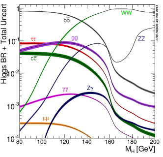
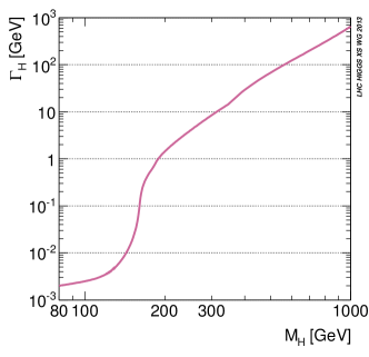
The Higgs branching ratios are shown in Fig. 3 for a SM Higgs boson of arbitrary mass. The width of the curves is an estimate of the theoretical uncertainties on the branching ratios. The branching ratios assume SM couplings and no new decay channels and include all known radiative corrections Dittmaier et al. (2011); de Florian et al. (2016a). Also shown in Fig. 3 is the Higgs total decay width as a function of Higgs mass. For , the total width is very small, . The reason is that the leading coupling entering the decays is the small bottom Yukawa coupling . Detailed predictions for the Standard Model branching ratios are given in Table 2. The sizes of the uncertainties on the Higgs branching ratios from various sources has been estimated in Ref. de Florian et al. (2016a).
3.5 Exotic and rare decays
Little is known about the interplay of the Higgs with the light fermionic degrees of freedom in the Standard Model that directly reflects the mass hierarchy of the three generations of fermions. The generation of the observed fermion mass hierarchy is a long-standing open question of particle physics and, contrary to the modeling of a light Higgs boson and electroweak symmetry breaking, only a small number of proposals exist to address the issue. Arguably the most famous among them is the Froggatt-Nielsen mechanism Froggatt and Nielsen (1979), although the original Froggatt-Nielsen model with the Higgs as a flavon is not phenomenologically viable.
It is possible that our naive SM picture of reflecting the mass hierarchy of the light fermions in their Yukawa couplings is not quite correct. The Higgs interactions could be a source of non-minimal flavor violation. If we allow such interactions, then approaches reminiscent of the Froggatt-Nielsen approach can explain the fermion mass hierarchy by making the Yukawa couplings Higgs-dependent Giudice and Lebedev (2008), which also breaks the SM relation which holds irrespective of the particle species. This scaling has been established only approximately so far, and measurements at the LHC are limited to the heavy particles of the Standard Model.
Unearthing the Higgs interactions with the light first and second generation of quarks is notoriously difficult. The hierarchy of Yukawas expected in the Standard Model indirectly generalizes to small branching probabilities of the Higgs into light fermions which systematically limits direct searches, see Eq.(A.23). The largest effect in the quark sector that qualifies as rare can be expected from , whose branching ratio in the Standard Model is 2.9% Denner et al. (2011). Studying the interactions of the Higgs with the lightest quark flavors is phenomenologically not possible as there is no ways to isolate these partons from the overwhelming QCD background. An observation of Higgs boson decays to charm quarks is also limited by large hadronic backgrounds at the LHC, as well as the strong trigger criteria required to facilitate the data taking in busy final states. However there are various possibilities linked to heavier quarks forming distinct meson final states.
One possibility is relying on distinctive signatures that are associated with the decay itself. For instance if an additional photon or boson is considered, , the charm quarks can recombine to form a vector meson which decays to muons about 6% of the time. Phenomenologically, vector boson-associated meson production leads to a highly distinctive and clean signature of two leptons recoiling against a photon, thus providing good a priori prospects to isolate this signature from the relatively small backgrounds that one expects here.
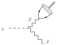
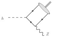
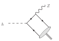
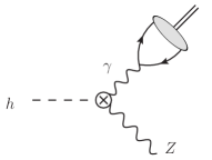
Interfering processes leading to an identical final state are , which also are enhanced close to the meson thresholds Bodwin et al. (2013, 2014), as well as prompt , see Fig. 4. In the Standard Model these contributions interfere destructively König and Neubert (2015); Alte et al. (2016) which can be used to place limits on new physics.
To discuss a specific and illustrative example, we consider the decay rates of a Higgs boson into a pseudo-scalar meson and a boson Alte et al. (2016)
| (A.37) |
where the form factor is dominated by contributions that are related to local hadronic matrix elements of the form
| (A.38) |
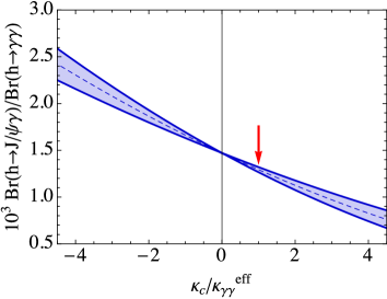
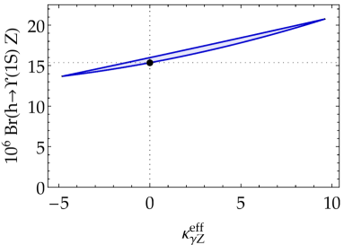
i.e. the probability to excite a pseudo-scalar meson from the strongly-interacting QCD vacuum (see also Sec. 5.5). stands for the axial-vector couplings of the boson to the corresponding quark. Contributions that are directly related to the charm quark coupling are suppressed . While limits can be placed on the charm quark coupling, see Fig. 5, and its parity structure (through angular correlations of the vector meson decay leptons Bhattacharya et al. (2014)), modifications of the interactions are typically more relevant. For the pseudo-scalar mesons, Ref. Alte et al. (2016) finds
| (A.39) |
The phenomenologically most relevant decays at the LHC are the Higgs decays involving heavy and -flavored vector mesons and a photon due to their final states and rates. The expected branching ratios in the Standard Model for the decays are König and Neubert (2015)
| (A.40) | ||||
| (A.41) | ||||
| (A.42) | ||||
| (A.43) |
where uncertainties related to decay constants and the theoretical uncertainty related to direct coupling of the Higgs to the meson and the dominant uncertainty from are included. Although the associated branching ratios are typically of the order of , a measurement of decays of the Higgs to mesons can provide a strong hint for the presence of new physics. For instance the decay of is highly sensitive to the presence of new interactions as can be seen from Fig. 5.
Most of the difficulties that arise when considering meson-associated decays of the Higgs boson are avoided when turning to rare leptonic Higgs decays as these are only impacted by QCD on the production side. A phenomenologically clear avenue to a rare leptonic Higgs decay is therefore . In the Standard Model, this decay has a branching ratio of Andersen et al. (2013)
| (A.44) |
Although the Higgs decay to muons is rare, muons are well-understood objects at colliders and the major limiting factor of analyses is the low signal yield of a resonance signal at .
A phenomenologically striking signature would be a lepton flavor violating Higgs decay Doršner et al. (2015). Such a situation can appear when the fermion mass generation is not aligned with the Yukawa couplings, for example in general two-Higgs doublet models. Seesaw mechanisms typically imply lepton flavor-violating Higgs couplings at the loop level since the mixing of neutrinos as part of a doublet will induce a lepton flavor misalignment of the Higgs couplings. For charged leptons, however, the associated branching ratios are very small, Arganda et al. (2005).
4 Implications for high scales
The biggest impact of the Higgs discovery on theoretical physics is that it structurally completes the Standard Model as a perturbative, renormalizable gauge theory. This means that we can use renormalization group evolution to connect very different energy regimes, from the QCD scale to Grand Unification or even the Planck scale. On the other hand, fundamental scalars in quantum field theory face two challenges, which we can explain in physics terms when we use an effective field theory picture: first, as discussed in Sec. 3.3 since the Higgs Yukawa couplings to fermions are proportional to the fermion mass, they do not fulfill the conditions necessary for the decoupling theorem to be valid, one of the fundamental assumptions we like to make in an effective field theory. As a side remark, SM-like Yukawa couplings larger than the top Yukawa immediately lead to nearby Landau poles where the Higgs self coupling blows up. Second, the hierarchy problem can be viewed as a quadratic dependence of the one-loop Higgs mass corrections on the exact value of the matching scale. This also contradicts our usual assumption that heavy physics does not affect predictions far below the matching scale. Both of those problems can, in practice, be ignored, because they do not invalidate our picture of the Standard Model as structurally complete. On the other hand, they might be able to lead us in our search for more fundamental theories at higher scales, and one of the main motivations of particle physicists is still to understand the most fundamental structures behind physics.
Before discussing renormalization group effects, we discuss a simple self-consistency criterion on the Higgs sector Llewellyn Smith (1973); Cornwall et al. (1974); Lee et al. (1977a, b); Chanowitz et al. (1978, 1979). It is based on the fact that the Higgs field and the Higgs potential in Eq.(A.3) also includes three Goldstone modes. In the high-energy limit, the Goldstone modes can be consistently identified with the longitudinal degrees of freedom of the weak bosons. For the charged Goldstone modes, defined as (cf Eq.(A.2)), we can compute the scattering amplitude for the process
| (A.45) |
approximating the scattering of physical, longitudinal gauge bosons at high energies. In the absence of a physical Higgs boson this scalar scattering process is perturbatively not unitary. A Higgs exchange in the -channel unitarizes the amplitude, but only if the Higgs field is light enough to contribute below the cut-off scale defined by perturbative unitarity violation. This translates into an upper limit on the Higgs mass, assuming that all Higgs and Goldstone interactions have SM strengths,
| (A.46) |
While the exact numerical value of this limit depends on the detailed interpretation, this relation has historically lead us to believe that the LHC had to either discover the Higgs boson or find some spectacular new physics effect. Given that the observed Higgs has approximately SM properties, longitudinal gauge boson scattering is approximately unitary, leaving little room for effects from strongly interacting gauge bosons at large energies. Similar unitarity arguments can be made based on Higgs-vector boson and fermion-vector boson scattering, but with a subleading effect on the Higgs mass limit. Unitarity arguments place strong restrictions on the parameters of BSM theories.
Using the renormalization group we can evolve the Higgs potential of the Standard Model to high energy scales. To good approximation, this evolution is driven by the self coupling , which to leading order runs as
| (A.47) |
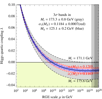
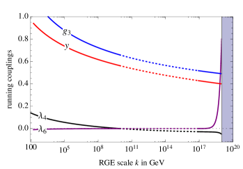
in terms of the top Yukawa and the gauge couplings and . There are two distinct features in this running. First, a large Higgs self-coupling will rapidly become stronger towards larger energy scales and hit a Landau pole, driven by the first term on the right side of Eq.(A.47). This behavior is also referred to as the triviality bound Maiani et al. (1978); Dashen and Neuberger (1983) and can be turned into an upper limit on the Higgs mass Lindner (1986). This limit is well above the observed Higgs mass of 125 GeV even when we require Landau poles to be absent all the way to the Planck scale. For smaller Higgs self-couplings, the negative top contribution drives the self-coupling negative at large energies Krive and Linde (1976); Krasnikov (1978); Lindner et al. (1989); Sher (1989); Holland (2005). In the absence of higher-dimensional operators of the kind shown in Eq.(A.6) the running self-coupling can ruin vacuum stability around GeV, as shown in the left panel of Fig. 6. If we include higher-dimensional operators, parameterized as
| (A.48) |
where is identical to of Eq.(A.6) and , we find that the scale of new physics curing the stability problem (the point where goes negative) can be a few orders of magnitude above this instability scale shown on the left of Fig. 6. However, in the right panel of Fig. 6 we see that even allowing for a metastability phase the new states should appear well below the GUT or Planck scale.
Renormalization group analyses become especially interesting when they feature infrared or ultraviolet fixed-points Schrempp and Wimmer (1996). This does not only include individual parameters, but also pseudo-fixed-point in ratios of parameters Pendleton and Ross (1981); Hill (1981), which effectively removes one parameter from the quantitative renormalization group analysis. In our case, the running of the top Yukawa coupling offers little information, but an interesting feature occurs in the running of the ratio of the Higgs self-coupling to the top Yukawa coupling Wetterich (1981). The ratio runs like
| (A.49) |
leading to an approximate infrared fixed-point in this ratio. The numerical value turns out to be very close to the observed values of the Higgs and top masses Shaposhnikov and Wetterich (2010). The observed values of the top and Higgs masses will generically be predicted by a wide range of parameter choices at some high-scale, implying a limited sensitivity of the relation between those two parameters to the details of the model in the ultraviolet. This still leaves open the question of why the electroweak scale is where it is.
Finally, baryogenesis is one of the great mysteries of particle physics. It can be related to the three Sakharov conditions Sakharov (1967), namely baryon number violation, and violation, and deviation from thermal equilibrium. None of the three conditions are convincingly fulfilled by the Standard Model. On the other hand, the second and third conditions can be linked to modified Higgs potentials. Concerning the third condition, it has been known for a long time that a renormalizable SM Higgs potential with a Higgs mass below roughly 60 GeV could lead to a strong first-order electroweak phase transition, leading to a deviation from thermal equilibrium around that time. Given the observed Higgs mass, there are two ways to turn the phase transition from second to first order Sher (1989): either we introduce additional scalar particles with masses around the Higgs or top mass or we modify the Higgs potential Grojean et al. (2005); Reichert et al. (2018).
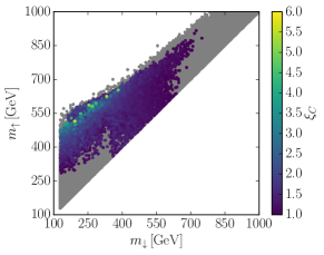
Following the first approach, the singlet extension discussed in Sec. 5.1 accommodates a strong first-order electroweak phase transition for specific choices of input parameters, typically GeV Profumo et al. (2015); Kurup and Perelstein (2017); Chen et al. (2017); Chiang et al. (2018). This possibility requires in Eq.(A.52) and places significant restrictions on the parameters of the potential. This first order electroweak phase transition does not occur in the -symmetric singlet model. A simple model which allows for -violation as well as a first-order phase transition is the complex 2HDM Basler et al. (2018). Unlike for the 2HDM discussed in Sec 5.2, the VEVs now have to be complex. In this case, the three neutral Higgs particles are not -eigenstates. In the type-I setup of the fermion sector all fermions couple to the same Higgs doublet. We can for example assume that the lightest of the three Higgs scalars is the observed SM-like Higgs boson. In that case the two heavier masses are free parameters of the model. In the left panel of Fig. 7 we show the critical parameter as a function of the two heavy BSM Higgs masses, where implies a strong first-order phase transition. Lighter masses are in general preferred. The complex 2HDM has the advantage that in addition it can provide the necessary -violation for electroweak baryogenesis. For the points shown in Fig. 7 this second condition is easiest, but not exclusively, fulfilled along the diagonal.
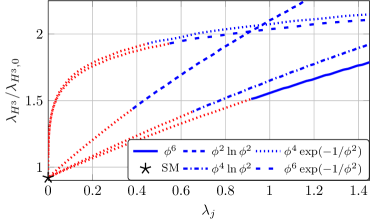
Using the second approach, the classic result is that a sufficiently large Wilson coefficient of the effective operator also leads to a strong first-order phase transition Grojean et al. (2005). This can be viewed as the main motivation for testing the Higgs self-coupling for order-one deviations. This relation between the triple Higgs coupling, accessible at the LHC, and the conditions for baryogenesis exists more generally. We can test it by expanding the SM Higgs potential in different ways,
| (A.50) | ||||||
The scale describes some kind of new physics. Neither the logarithmic nor the exponential potentials can be expanded around . From a more general viewpoint, the set of power law, logarithmic and exponential potential functions does not only reflect the physics structures arising from local vertex expansions, one-loop determinants or semi-classical approximations. It also includes the set of functions to be expected if the effective potential permits a potentially resurgent trans-series expansion Dunne and Unsal (2012). In the right panel of Fig. 7 we show the nature of the electroweak phase transition as a function of the underlying model parameters, directly correlated with the size of the physical Higgs self-coupling. For all cases we observe that a strong first-order phase transition is only possible for Higgs self-couplings significantly above the SM value. Specifically, the HL-LHC should be able to conclusively test these parameter regions and confirm or rule out the possibility of electroweak baryogenesis in a very model-independent manner.
5 Extended Higgs sectors
Perturbative extensions of the Standard Model are strongly restricted by experimental constraints, cosmological considerations, and theoretical limitations. New particles can be scalars, fermions, or gauge bosons. From a Higgs physics perspective, new fermions mostly enter the loop-induced Higgs decays described in Sec. 3 and the gluon fusion production rate described in Sec. 1. The requirement that these rates have close to the observed rates forbids a chiral generation Kribs et al. (2007); Denner et al. (2012a). Extended gauge sectors are a key ingredient of many strongly interacting extensions described in Sec. 5.5. Similarly, extended scalar potentials are a generic extension of the Standard Model and have direct impacts on Higgs physics. They can, but do not have to, be related to a broader ultraviolet completion of the Standard Model.
For a scalar extension of the Standard Model, we classify the new scalar fields by their representation of . This representation is directly linked to the main constraint on many such extensions, namely electroweak precision constraints. From Sec. 4 we know that the constraints typically require a global custodial symmetry at least at tree level. For additional scalar or Higgs fields with weak isospins , hypercharges , and vacuum expectation values we find Langacker (1981); Chen et al. (2006); Cheng et al. (1974)
| (A.51) |
where for a doublet and for a singlet. This means that aside from additional scalar singlets, models with additional Higgs doublets also respect custodial symmetry at tree level. Higher representations, like triplets, typically force us to live with very strong constraints Barger et al. (2009).
5.1 Additional singlet
The addition of a real scalar singlet, , is the simplest extension of the minimal Higgs sector, with very few free parameters, allowing for definite predictions of Higgs signals. The most general scalar interactions are Silveira and Zee (1985); O’Connell et al. (2007); Bowen et al. (2007); Pruna and Robens (2013); Espinosa et al. (2012); Dawson and Lewis (2015)
| (A.52) |
Based on this form of the potential, the VEV of can always be set to by shifts in the input parameters. After spontaneous symmetry breaking, the neutral component of and mix to form the physical states and . Explicit expressions for the masses, and , and the mixing angle that diagonalizes the scalar mass matrix, in terms of the parameters of Eq.(A.52) can be found in the appendices of Ref. Chen et al. (2015a) or Ref. López-Val et al. (2013). We usually assume the lighter mass eigenstate is the observed SM-like particle, . This implies that all LHC production rates are suppressed by , while the branching ratios are unchanged. This kind of model allows for a particularly easy interpretation of the global Higgs coupling analyses described in Sec. 6. If the new scalar is light, GeV, and the heavier scalar, , is the observed Higgs boson, the model predicts Higgs-to-Higgs decays with the partial width
| (A.53) |
in terms of the physical triple-Higgs coupling , which can be extracted from the potential Espinosa et al. (2012).
In the -symmetric version of the theory there is a symmetry under , and it is in general not possible to set . Whenever there are two non-zero VEVs, as is the case in this example, we define the ratio of the two VEVs as . The theory is completely described by the parameters,
| (A.54) |
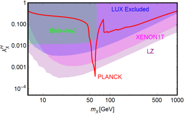
A Higgs portal dark matter model Silveira and Zee (1985); McDonald (1994); Burgess et al. (2001) arises in the -symmetric scenario when we adjust the parameters such that is 0 Binoth and van der Bij (1997); Schabinger and Wells (2005); Patt and Wilczek (2006); Lebedev et al. (2012). The entire dark matter model is then described by three parameters: the singlet mass term , the portal coupling , and the singlet self-interactions . For most observables, the singlet self-interaction is phenomenologically irrelevant over a wide range of model parameters. The portal coupling determines, for example, the dark matter annihilation rate or the scattering rate with nucleons. The interaction relevant for direct detection is mediated by the SM Higgs boson, coupling to virtual top quark loops generated by the non-relativistic gluon content of the nucleus Shifman et al. (1978). Away from the pole condition and for reasonably light dark matter masses, this rules out the model as an explanation of the observed relic density. Some current and future constraints including the relic density constraints and direct detection experiments are shown in Fig. 8.
For a light enough dark matter state, the Higgs-to-Higgs decays shown in Eq.(A.53) lead to invisible Higgs decays Shrock and Suzuki (1982) at the LHC, as described in Sec. 2. In Fig. 8 we see that invisible Higgs decays can probe the parameter regions which lead the to correct relic density, provided that the dark matter is lighter than the SM Higgs boson. Unfortunately, this parameter region is, for the simple singlet extension, essentially ruled out by direct detection experiments. In the opposite case, where the dark matter scalar is heavier than we will not be able to extract the small production rate from the backgrounds. If the new singlet scalar becomes even heavier, the Higgs-to-Higgs decays shown in Eq.(A.53) correspond to a decay of the heavy new state and makes an important resonance contribution to , as discussed in Sec. 2.1.
5.2 Additional doublet
The two Higgs doublet model (2HDM) Haber et al. (1979); Branco et al. (2012) adds a second doublet with weak hypercharge one. This way it allows for -violation and a complex vacuum structure Gunion and Haber (2005), can be linked to neutrino masses Ma (2006), electroweak baryogenesis Cline et al. (1996); Fromme et al. (2006), or dark matter Gong et al. (2012). The general -invariant renormalizable potential reads
| (A.55) |
Hermiticity of the potential requires and to be real. The parameters and can be complex, in which case all neutral Higgs fields will mix and define physical fields that are no longer -eigenstates. We only illustrate the -even case, for a comprehensive discussion of the -violating case see Pilaftsis and Wagner (1999).
If we consider the 2HDM to be a valid ultraviolet completion of the Standard Model, the vacuum must be stable. This can be ensured by requiring Gunion and Haber (2003); Kanemura et al. (1999)
| (A.56) |
Electroweak symmetry breaking, as described in Sec. 2, now requires . The remaining free parameter is . The physical spectrum consists of two neutral -even scalars , one neutral -odd scalar , and a charged scalar . The two mass eigenstates and arise from a rotation by the angle ,
| (A.57) |
and the -odd and charged Higgs masses can be easily extracted from the potential,
| (A.58) |
and . The range of possible spectra includes compressed masses (), twisted masses (), a single mass hierarchy (), or multiple mass hierarchies (), each of which have quite different phenomenologyCraig et al. (2015). The limit is termed the decoupling limit, and in this limit the couplings of approach those of the SM Higgs boson Gunion and Haber (2003); Carena et al. (2014); Bhupal Dev and Pilaftsis (2014).
Since custodial symmetry strongly constrains extended Higgs sectors, we can assign the Higgs masses in the 2HDM accordingly. Barring fine-tuning in the mixing angles, two scenarios generally respect custodial symmetry. First, a compressed mass spectrum with only moderately split Higgs masses directly follows the pattern of Eq.(A.51). For degenerate masses the contributions to the electroweak precision parameters at tree level are . Second, for a light SM-like Higgs with mass-degenerate heavy companions all Higgs states fall into the singlet and triplet representations of the custodial symmetry group ,
| (A.59) |
typically with a rich vacuum structure, see Battye et al. (2011); Pilaftsis (2012). We can integrate out all heavy Higgs fields simultaneously and retrieve an effective field theory in terms of only. This gives in the limit of heavy additional Higgs states He et al. (2001)
| (A.60) |
The gauge sector of all 2HDM setups is especially simple. The couplings of the light Higgs to the weak bosons always scale like
| (A.61) |
where we define as systematically introduced in Sec. 7.1, and possible pre-factors drop out of the ratio. The decoupling limit is given by . On the side of the Yukawa couplings, the 2HDM setup offers a lot of freedom. In the Standard Model, for example, a global symmetry group leaves the CKM matrix invariant and guarantees the absence of tree-level FCNCs. The symmetry is broken by large Yukawa couplings. This protection against FCNCs does not hold in the presence of a second Higgs doublet Hall and Wise (1981). Natural flavor conservation imposes a global flavor-blind symmetry and requires that any fermion family can couple to only one Higgs doublet. This simple Higgs flavor symmetry satisfies the Glashow-Weinberg theorem Glashow and Weinberg (1977), forbids the mass term and the self interactions , and defines four canonical setups for the couplings of and to fermions:
-
•
type-I, where all fermions only couple to ;
-
•
type-II, where up-type (down-type) fermions couple exclusively to ();
-
•
lepton–specific, with a type-I quark sector and a type-II lepton sector;
-
•
flipped, with a type-II quark sector and a type-I lepton sector.
If we extend the flavor symmetry to the Yukawa sector as a Peccei-Quinn (PQ) symmetry, it removes all sources of tree-level FCNC interactions. The mass splitting between the and is controlled by the size of the PQ-breaking terms and . Yukawa structures respecting natural flavor conservation are a special case of a class of models in which tree-level FCNCs are largely suppressed via minimal flavor violation D’Ambrosio et al. (2002); Dery et al. (2013). In the 2HDM realization Pich and Tuzon (2009) the fermions couple to both Higgs doublets with aligned Yukawa matrices, i.e. linked to one another by linear shifts ,
| (A.62) |
with as defined in Eq.(A.17). This way the fermion masses and Yukawa matrices are diagonalized simultaneously. We can parameterize the shifts in terms of angles Davidson and Haber (2005) modifying the bottom and tau Yukawas
| (A.63) |
The neutral Higgs couplings to fermions in the 2HDM in terms of the SM Higgs couplings are given in Tab. 3. For the light SM-like Higgs couplings to fermions there exist two sources of coupling modifications: first, the fermionic 2HDM mixing structure includes a -odd gauge boson . This leads to non-trivial ratios of functions of and . Second, in the aligned model where , the couplings to the top quark, bottom quark, and tau can be varied independently. Note that the aligned limit can be realized without the decoupling of and .
| 0 | |||
When we embed the extended Higgs sector in a perturbative ultraviolet completion of the Standard Model, we need to ensure that the Landau poles of all Higgs self-couplings lie outside the validity range of our model. For weakly interacting models, a stronger constraint arises from perturbative unitarity Lee et al. (1977b). The leading effects at high energies constrain the combinations Casalbuoni et al. (1986, 1988); Kanemura et al. (1993); Akeroyd et al. (2000); Gunion and Haber (2003); Ginzburg and Ivanov (2005); Osland et al. (2008); Pruna and Robens (2013) of parameters in the scalar potential given in Eq.(A.55),
| (A.64) | ||||||
to remain smaller than unity. Assuming the usual 2HDM pattern imposes a set of sum rules Llewellyn Smith (1973); Cornwall et al. (1973, 1974); Weldon (1984); Gunion et al. (1991a)
| (A.65) | ||||||
with . These tree–level sum rules imply that the Higgs couplings to weak bosons can be at most as strong as in the Standard Model. Moreover, all vertices containing at least one gauge boson and exactly one heavy Higgs field are proportional to . Finally, the Yukawa coupling comes with an additional factor . According to the sum rule, at least one of the -even Yukawa couplings can therefore lie above .
If, in addition, we require that all 2HDM Yukawas remain perturbative at the weak scale, , we find for all natural flavor-conserving models, for type-II and flipped models, and in the lepton–specific case Chen and Dawson (2013).
Interesting variations of the 2HDM are dark portal or inert doublet models Deshpande and Ma (1978); Ma (2006); Majumdar and Ghosal (2008); Barbieri et al. (2006); Lopez Honorez et al. (2007). They require a -symmetry in Eq.(A.55), under which one doublet transforms as odd. For the 2HDM potential given in Eq.(A.55) this means that and . The new, -odd doublet does not participate in electroweak symmetry breaking. This means that it can only interact with SM particles when it appears twice in the vertex. For the fermions such an interaction would not be renormalizable, but for the weak bosons it is induced by the covariant interactions in the kinetic term. The corresponding scalar or pseudo-scalar dark matter agent therefore couples to the SM particles through the usual Higgs portal discussed in Sec. 5.1, complemented by a possible direct annihilation to or pairs.
5.3 Additional triplet
Naive triplet extensions of the SM Higgs sector tend to be in violent conflict with electroweak precision data already at tree level, Eq.(A.51). There are three ways to deal with this: (i) live with very strong model constraints; (ii) carefully align different triplet Higgs fields, like in the Georgi-Machacek model Georgi and Machacek (1985), at the price of additional fine-tuning Gunion et al. (1991b); or (iii) combine exotic representations Hisano and Tsumura (2013). Theoretical motivations for triplet models are provided by left-right symmetries Mohapatra and Pati (1975a, b); Senjanovic and Mohapatra (1975) or models for neutrino mass generation Konetschny and Kummer (1977); Magg and Wetterich (1980); Cheng and Li (1980). Interesting implications have also been highlighted in the context of non-minimal SUSY extensions Delgado et al. (2013).
There are two possible hypercharge assignments for an triplet:
-
•
, real scalar
(A.66) -
•
, complex scalar
(A.67)
The interactions of the triplets with the gauge kinetic terms generates contributions to the gauge boson masses,
| (A.68) |
where is the doublet VEV. The addition of triplet scalars contributes to custodial symmetry breaking,
| (A.69) |
From this formula, we see that choosing protects the model from constraints arising due to electroweak precision data at tree level. The Georgi-Machacek model Georgi and Machacek (1985); Hartling et al. (2015); Englert et al. (2013a) realizes this mechanism with the help of a real scalar triplet and a complex scalar triplet, in addition to a doublet which is still needed for fermion mass generation, and predicts at tree level. The physical spectrum includes two -even scalars , one -odd scalar , one singly charged scalar , and one doubly-charged state . This way we define three mixing angles in the scalar sector, the usual angle in the -even scalar sector, plus the angle in the charged scalar sector and the angle in the -odd scalar sector. The heavy ‘states can be combined into a heavy triplet, minimizing the tree-level breaking of the custodial symmetry,
| (A.70) |
In terms of the common VEV , the and masses are both given by the same combination . Custodial symmetry then acts in the triplet representation on Eq.(A.70) similar to Eq.(A.20).
A structural difference between the doublet and triplet extensions is that the triplet models predict tree-level couplings Han et al. (2006). The smoking gun at the LHC for complex triplets is the doubly charged Higgs, produced either in a Drell-Yan process or in weak boson fusion through a coupling. These exotic couplings are directly related to the triplet character of the vacuum expectation value and they scale with a characteristic angle .
| extension | model | ||||||||
|---|---|---|---|---|---|---|---|---|---|
| universal | non-universal | universal | non-universal | ||||||
| singlet | inert () | ||||||||
| EWSB () | |||||||||
| doublet | inert () | ||||||||
| type-I | |||||||||
| type-II-IV | , | ||||||||
| aligned, MFV | |||||||||
| triplet | complex scalar | ||||||||
In the spirit of precision Higgs physics, the key question for all extended Higgs sectors is how they affect the SM-like Higgs couplings. We parameterize the coupling deviations for the SM-like Higgs from the Standard Model predictions as Lafaye et al. (2009)
| (A.71) |
We start with the simple coupling structures to gauge bosons given in Table 4. For the singlet and doublet extensions, the universal coupling modifications are simply a rotation by an angle or . The implication is that extended Higgs sectors can only reduce the couplings to gauge bosons. In addition, non-universal fermion–mediated or Higgs–mediated loop contributions can change the couplings to gauge bosons in either direction.
The SM-like fermionic coupling variations are much more model-dependent. While the singlet model is fully described by one mixing angle, the aligned 2HDM model allows for essentially free coupling modifications with either sign.
Finally, Higgs interactions with photons and gluons are generated by loops already in the Standard Model. For the gluon case this requires colored states, so we can immediately apply the modified quark Yukawa patterns of an extended Higgs sector. The photon coupling depends on the three heavy Yukawa couplings and on , but also receives corrections due to new charged scalars in the Higgs sector. The effect of additional states is relatively enhanced as it spoils to the destructive interference between the leading top and contributions in the Standard Model Kribs et al. (2007).
5.4 (N)MSSM
Ultraviolet extensions of the Standard Model predicting an extended Higgs sector include supersymmetric models Gunion and Haber (1986a, b). The reason is that in the Standard Model, we use and to give mass to the up-type and down-type fermions, while in a supersymmetric Lagrangian we are not allowed to use conjugate super-fields. The way out is to give mass to the fermions with two Higgs doublets, and . As in any 2HDM setup, the two VEVs combined give the weak boson masses, implying or .
There are three kinds of contributions to the minimal supersymmetric Higgs potential. First, -terms from the SUSY-conserving scalar potential include scalar quark interactions proportional to Yukawa couplings, as well as Higgs mass terms proportional to a new parameter . Second, gauge–coupling mediated SUSY-conserving terms lead to four-scalar interactions proportional to SM gauge couplings. The sign of the terms in the Lagrangian is indeed predicted to be negative. Finally, Higgs masses appear as soft breaking parameters. The -term gauge couplings determine the Higgs potential of the MSSM Chung et al. (2005); Bhattacharyya et al. (2018), cf. Eq.(A.55),
| (A.72) |
The main feature of the MSSM setup is that these self-couplings are limited from above, implying an upper limit on the lighter of the two -even Higgs states.
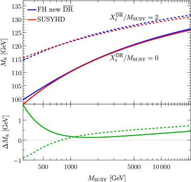
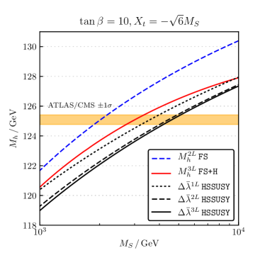
At tree level the entire Higgs sector is determined by two parameters, often chosen as and . Typically, the MSSM Higgs sector shows a mass hierarchy , in line with the generic hierarchical benchmark. Custodial symmetry and tree-level FCNC suppression are guaranteed. The lighter -even mass is then predicted in terms of the MSSM parameters, and the observed value of GeV requires large quantum corrections Haber et al. (1997); Degrassi et al. (2003); Hahn et al. (2009). Given the LHC constraints for example on the top squarks, the corresponding calculation at the required precision is plagued by sizable logarithms . We show the comparison between logarithms-enhanced fixed-order prediction and the EFT-based prediction Pardo Vega and Villadoro (2015) in the left panel of Fig. 9, indicating an agreement at the 1 GeV level even for heavy supersymmetric states. In the right panel of Fig. 9 we show the results from an EFT-enhanced 4-loop prediction, compared to the fixed order 2-loop (FS) and 3-loop (FS+H) results. For large mixing in the supersymmetric stop sector, the EFT corrections are typically large and negative, and there exists a sizeable dependence on the matching to the fixed-order 3-loop results.
In supersymmetric models with -parity, the lightest superpartner serves as a dark matter candidate. In many cases, this is the lightest neutralino, , a Majorana fermion coupling to the Higgs bosons through gaugino-higgsino mixing. The Higgs sector in the MSSM provides three dark matter mediators, the light Higgs boson as well as the -even and -odd heavy Higgs bosons. In all three cases, the observed relic density combined with a standard thermal production process requires an on-shell condition , similar to the scalar Higgs portal discussed in Sec. 5.1. In contrast to the scalar case shown in Fig. 8 the SM-Higgs portal with Majorana fermion dark matter will be fully accessible by the next generation of direct detection experiments.
Adding singlets to the supersymmetric 2HDM setup hardly changes its main LHC features in the Higgs sector, but it can completely change the neutralino dark matter phenomenology Ellwanger et al. (2010); Maniatis (2010). The main virtue of the NMSSM is that it generates the non-supersymmetric higgsino mass term through a singlet contribution in the Higgs potential and the corresponding singlet VEV. The particle spectrum now includes three neutral -even states and two neutral -odd scalars. A SM-like Higgs boson can be realized for large and small values. In this case the two lightest mass eigenstates are typically close in mass.
If, in the spirit of the NMSSM, we assume that the additional singlet develops a VEV, we find a light Higgs state with couplings
| (A.73) |
where we assume a type-I 2HDM structure. The 2HDM interaction pattern is simply rescaled.
A major difference between the MSSM and the NMSSM appears in the dark matter sector. On the one hand, the additional fermionic gauge singlet (singlino) present in the NMSSM gives us more freedom to adjust the parameters of the neutralino sector. On the other hand, the additional -even and -odd singlet field can be light with sizeable couplings to the singlino and reduced couplings to the Standard Model. This turns them into promising dark matter mediators for dark matter neutralinos as light as a few GeV and not accessible to nuclear recoil direct detection experiments.
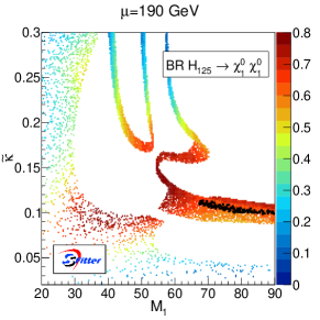
Light NMSSM neutralinos are one of the few actual models which motivate invisible Higgs searches. Even including all other experimental constraints, the invisible branching ratio of the SM-like Higgs can vastly exceed the current experimental limits. In Fig. 10 we show the predicted invisible branching ratio for a slice in the MSSM parameter space with fixed Higgsino mass. The parameter is given by the singlino mass parameter normalized by and is the usual bino mass. All shown points predict the correct relic density, and the black dots explain the Fermi galactic center excess. The predicted invisible branching ratios can be as large as 70%, strongly correlated with signal rates in indirect dark matter detection.
5.5 Strong couplings
Strong interactions are typically considered as viable contenders for explaining a hierarchy between the electroweak scale and any other UV scale which resolves the Standard Model into a more fundamental theory. We do not yet know if the Higgs is a fundamental particle or a composite particle resulting from some strong dynamics, provided the strong dynamics predicts a very narrow lightest particle. Theories of strong electroweak symmetry breaking take inspiration from the precedent of QCD as one well-understood theory of a strong interactions with approximate global symmetry Scherer (2003). Simply “copying” QCD at higher scales, referred to as Technicolor Eichten and Lane (1980); Farhi and Susskind (1981), has become increasingly difficult after the Higgs discovery, as obtaining a light SM Higgs-like particle from a strongly-interacting sector with a significant mass gap between the high scale physics and the weak scale does not follow the QCD paradigm Donoghue et al. (1989); Gasser and Leutwyler (1984). Insights from first principle lattice calculations Aoki et al. (2014) are far from straightforward, in particular because the symmetry and matter content of realistic candidate theories of electroweak type interactions is much bigger than that of QCD.
An approach that takes the pion mass splitting as a key inspiration realizes the light SM-like Higgs boson as a composite pseudo-Nambu Goldstone field. The pion is governed by strong QCD effects in the presence of small quark masses, and falls outside the perturbative realm. The weak gauging of QED, however, opens up the possibility of using perturbative techniques within a strongly-interacting picture, leading to perturbative predictions which are remarkably close to the actual experimental findings. Concretely, this utilizes the weak gauging of QED into the
| (A.74) |
symmetry of 2-flavor QCD in the chiral limit, with symmetry breaking induced by the strong dynamics of QCD.
As the axial symmetries associated with the currents
| (A.75) |
are broken, there are 3 associated massless Nambu Goldstone fields. The associated broken symmetry transformations gives these fields their pseudo-scalar quantum numbers. As the fundamental quark masses can be chosen to be zero, we still have .
The currents of Eq.(A.75) have the right quantum numbers to excite the pseudo-scalar state with momentum from the vacuum
| (A.76) |
with the characteristic pion decay constant (which can be related to the quark condensate in the strongly interacting vacuum). Axial current conservation then implies , i.e. the partially-conserved axial current hypothesis. Using Eq.(A.76) we can express general Green’s functions, e.g.
| (A.77) |
Under the assumption that the low energy behavior of the Greens functions is dominated by the pseudoscalar mesons (pion pole-dominance), we can introduce an interpolating field
| (A.78) |
when transitioning to the strongly interacting picture. The detailed investigation (including the strange quarks) of Ref. Gasser and Leutwyler (1985) shows that exponentials of these interpolating fields
| (A.79) |
provide an appropriate way of capturing the dynamics in an effective theory. This can be traced to the particular linear and non-linear symmetry transformation properties of Coleman et al. (1969); Callan et al. (1969) under the transformations. A suitable low energy effective theory for the pions is then given by
| (A.80) | ||||
| (A.81) |
where the ellipses refer to higher order terms in the low momentum expansion.
The presence of gauge interactions external to the strong sector and associated with only a subgroup means that the true vacuum of the theory can be misaligned from the the tree-level vacuum that conserves : gauging a subgroup means explicitly breaking the global symmetry. Treating the gauging as as perturbative effect we can compute the effective effective one-loop pion potential from photon contributions Contino (2011); Panico and Wulzer (2016), yielding
| (A.82) |
with . The dimension 4 constant
| (A.83) |
is related to an correlator related to the currents of Eq.(A.75)
| (A.84) |
It is straightforward to express in terms of the axial current correlators (cf. Eq.(A.75)) as well as analogously introduced vector current correlators , and analyze its low energy behavior with Eq.(A.77),
| (A.85) |
as the vector currents are not broken in the QCD vacuum. is strictly positive for vector-like confining gauge theories Witten (1983) and the high energy behavior can be estimated in QCD using the Weinberg sum rules Weinberg (1967b) and the vector meson dominance approximation Sakurai (1960), which means that the first vector mesons dominate the phenomenology expressed by the Weinberg sum rules. The Weinberg sum rules imply that the high-energy behavior of is well-behaved and the integral converges as for large .
A positive means that the pion potential is minimized for and the vacuum is dynamically aligned in the gauge symmetry-conserving direction; the photon stays massless. The charged pion, however, obtains a non-zero radiative mass Das et al. (1967) turning it into a pseudo-Nambu Goldstone Boson (pNGB)
| (A.86) |
where are the first (and dominant) vector and axial vector resonances with masses of 770 MeV and 1260 MeV, respectively. In this formulation the neutral pion stays massless as chiral symmetry is only broken by the non-zero quark masses that are neglected here. Even when these effects are included, the mass splitting between the charged and uncharged pions is dominated by the QED radiative effects, in good agreement with the experimentally observed splitting of 4.6 MeV.
| Model | |||||
|---|---|---|---|---|---|
| MCHM4 | |||||
| MCHM5 |
Composite Higgs models aim at adopting the above strategy to the electroweak case. This is not straightforward: we have to properly break electroweak symmetry rather than only introducing parametrically small masses for the Higgs boson as a pNGB; no massless states should remain in the spectrum. A key ingredient of the solution is partial compositeness Kaplan (1991); Contino et al. (2007a) of heavy fermions, which explains the observed mass hierarchy of fermions in terms of mixing with baryons of the strongly interacting sector through (extended) hypercolor interactions. Partial compositeness introduces new, vacuum-misaligning one-loop terms to the effective potential, which then takes a schematic form Contino et al. (2003); Agashe et al. (2005); Contino (2011)
| (A.87) |
Here is the analogue of the above pion decay constant for the electroweak symmetry breaking case and the parameter that measures the radiatively-generated electroweak scale in units of
| (A.88) |
The dimensionless coefficients are related to combinations of two-point and four-point correlator functions of the microscopic theory similar to Eq.(A.84), see DeGrand et al. (2016); Golterman and Shamir (2015, 2018); Del Debbio et al. (2017). Calculating these functions using lattice simulations is possible in principle, however, for realistic theories with an enlarged matter and symmetry content Ferretti (2016) this is unfortunately beyond the current state of the art although significant progress has already been achieved Ayyar et al. (2018a, b, c).
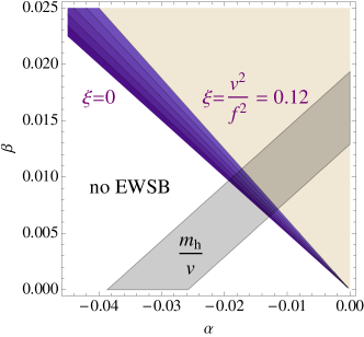
Although concrete UV completions of composite Higgs scenarios are currently unclear (this also includes the validity of the QCD-specific assumptions made above for the pion example), using the effective low energy constants and their relation to measurable quantities like the Higgs mass and the Higgs couplings, constraints can formulated which can inform future lattice investigations. In particular, the condition for electroweak symmetry breaking requires and the Higgs mass measured in units of the electroweak vacuum expectation value correlates and
| (A.89) |
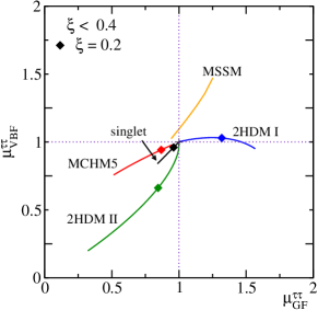
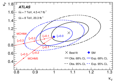
The parameter parameterizes the differences in Higgs phenomenology compared to the Standard Model. Scenarios, which are typically adopted as benchmarks of a pNGB origin of electroweak symmetry breaking are models based on a non-linear sigma model Agashe and Contino (2006); Barbieri et al. (2007); Bellazzini et al. (2014), analogous to Eq.(A.79), with fermions either embedded in the four-dimensional spinorial or five-dimensional fundamental representation of . These models are referred to as minimal composite Higgs models MCHM4 and MCHM5. They imply different Higgs interactions with SM fermions, as tabulated in Tab. 5 Giudice et al. (2007). A constraint on can therefore be used to contrast predictions from specific UV models, Fig. 11. MCHM5 is a particularly well-motivated phenomenological candidate as it includes enough symmetry to satisfy LEP constraints Contino et al. (2007b) and a range of viable parameter choices consistent with LHC data can be formulated Gillioz et al. (2012). In the right panel of Fig. 11 we show how this specific model can be identified based on LHC rate modifications. In Fig. 12 we show an ATLAS interpretation of single Higgs measurements in these models Aad et al. (2015b).
Other scenarios of strong interactions that approach the light nature of the Higgs boson from a different angle are theories of collective symmetry breaking, known as Little Higgs theories Arkani-Hamed et al. (2002); Csaki et al. (2003), where the Higgs is interpreted as a pNGB that typically (but not necessarily) arises through breaking of a product group of symmetries. These models have been reviewed in other places in detail Schmaltz and Tucker-Smith (2005); Perelstein (2007). Other versions of pNGB type Higgs physics include Twin Higgs models Chacko et al. (2006) as well as models motivated from holography Contino et al. (2003). Scalar sectors in these kinds of models typically share phenomenological similarities with the 2HDM or the Georgi-Machacek model, as discussed in Sec. 5.3, because they form representations of by construction. Current constraints from a range of existing searches are loose, in particular when the triplets do not contribute to electroweak symmetry breaking Del Debbio et al. (2017).
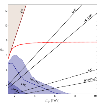
Minimal models like MCHM4 and MCHM5 have currently no known (non-supersymmetric) UV completion. Extended theories Ferretti and Karateev (2014); Ferretti (2014); Cacciapaglia and Sannino (2016); Ferretti (2016) typically include other exotic states on top of top and bottom quark partners Pomarol and Riva (2012); De Simone et al. (2013); Matsedonskyi et al. (2014), such hyper-pions Belyaev et al. (2017), axion-like states Belyaev et al. (2017), (doubly) charged Higgs bosons Del Debbio et al. (2017) and vectors Marzocca et al. (2012); Thamm et al. (2015). Searches for the heavy particle in these models typically provide complementary information from measurement of Higgs couplings. In a model with heavy vector resonances of mass, and coupling , the parameter and typically limits are shown in the right panel of Fig. 12.
6 Characterizing the Higgs boson
Understanding the properties of the SM-like Higgs boson and the symmetry structure of the Higgs Lagrangian is the first task when we want to interpret LHC Higgs measurements in terms of a quantum field theory.
6.1 Mass and Lifetime
The mass of the Higgs boson was the only unknown parameter of the Standard Model prior to its discovery. Electroweak symmetry breaking puts the Higgs mass at the center of the reliability of the electroweak series expansion. For instance, the parameter that measures custodial isospin is logarithmically dependent on the Higgs mass. This together with the constraints on the parameter allowed tight constraints to be put on the mass of the Higgs , which forced these logarithms to be small, therefore requiring electroweak physics to follow the standard perturbative QFT paradigm. More concrete evidence of the Higgs mass being the “order parameter” of the convergence of the electroweak series expansion can derived from the Higgs width Goria et al. (2012): for Higgs masses approaching the threshold is about a factor 2 smaller than fermions. As the decay widths are related to imaginary parts of the Higgs self-energy, the importance of 4 body decays compared to 2 body decays can be related to 3 loop diagrams being equally important as one loop contributions for such Higgs masses, which signalizes a slow convergence.
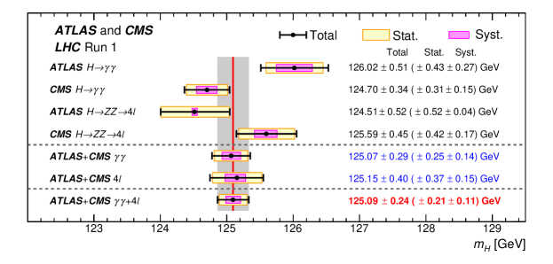
Because the Higgs mass reach was the limiting factor in LEP searches, a SM-like Higgs is excluded by LEP for GeV at 95% C.L. Barate et al. (2003). At the LHC the Higgs mass crucially impacts signal yields. Hence, studying the observed signal rates as a function of the Higgs boson mass can be used to constrain the Higgs mass, as done in a combined fit of ATLAS and CMS data Aad et al. (2015a) for 7 TeV and 8 TeV data. The combination of ATLAS and CMS measurements in the and channels gives the currently best measurement on the Higgs mass in the Standard Model, Fig. 13,
| (A.90) |
The Higgs width or lifetime is a crucial parameter for BSM searches. For instance, it can be related to dark matter through scalar extensions as described above. With a SM value of for the 125 GeV Higgs boson, the width is much smaller than the experimental resolution of about and line-shape analyses similar to the boson are not immediately promising at the LHC. A range of proposals have been advertised to circumvent this limitation through on-shell interference effects Dixon and Li (2013); Dixon and Siu (2003); Martin (2012, 2013); Coradeschi et al. (2015); Campbell et al. (2017). They rely on improved experimental systematics or on correlating different regions of phase space Caola and Melnikov (2013); Campbell et al. (2014a, b); Englert and Spannowsky (2014). It is worth mentioning that most of the Monte Carlo tools relevant for Higgs and electroweak physics at the LHC rely on Nowakowski and Pilaftsis (1993); Argyres et al. (1995); Papavassiliou and Pilaftsis (1998a, b); Denner and Dittmaier (2006); Passarino et al. (2010). The naive Breit-Wigner hypothesis that is typically employed in these simulations cannot be supported when the width becomes large Passarino (2014); Goria et al. (2012).
The basic idea for extracting the Higgs width from off-shell Higgs production employs properties of the longitudinal -polarizations Kauer and Passarino (2012); Caola and Melnikov (2013); Kauer (2013). The process
| (A.91) |
contains contributions from the Higgs resonance, but also contributions independent of the resonance. From the Breit-Wigner propagator, , we know that the Higgs amplitude squared and the interference with the continuum background on and above the resonance give very different information on the Higgs width. The analysis idea is that by measuring the rate above and on the resonance we can extract information about the Higgs width. The advantage of the decay is that at TeV approximately of the total cross section has , offering enough off-shell Higgs events for a measurement. ATLAS and CMS have used this technique to place limits on the Higgs width Khachatryan et al. (2014); Aad et al. (2015c),
| (A.92) |
However, the Higgs coupling to gluons is loop-induced and can have a non-trivial dependence on all masses involved Gainer et al. (2015); Englert et al. (2015a); Cacciapaglia et al. (2014); Ghezzi et al. (2014); Azatov et al. (2015a); Buschmann et al. (2015); Logan (2015), and so the extraction the Higgs width requires us to make (often implicit) assumptions that all interactions are those of the Standard Model.
6.2 Spin
An obvious first step after the Higgs boson discovery was to establish the new scalar’s spin, or constrain the spin-associated interaction terms of an effective Lagrangian. The effective interactions that were used to constrain such couplings or to contrast with the SM Higgs in simple hypothesis tests need to be understood as straw-man proposals. They are not motivated by actual models or theories, and they typically cannot be understood in terms of renormalizable theories. Interaction terms are typically considered for spin for Higgs imposters . We focus on the -even case as an example, for which the following interaction terms can be considered Englert et al. (2010); Artoisenet et al. (2013a); Maltoni et al. (2014); Gainer et al. (2015)).
Spin 0:
| (A.93) |
Spin 1:
| (A.94) |
Spin 2:
| (A.95) |
where the energy momentum-tensor parts of the fermions, gluons and vector bosons can be found in Han et al. (1999); Hagiwara et al. (2008). All ad-hoc parameters are free couplings associated with the (higher-dimensional) interactions.
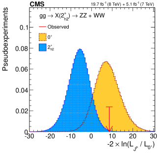
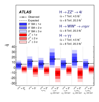
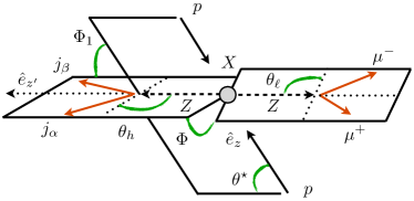
There are various ways to constrain the above interaction terms, including the classic study of angular decay distribution shapes in various channels Dell’Aquila and Nelson (1986a, b); Collins and Soper (1977); Nelson (1988); Miller et al. (2001); Choi et al. (2003); De Rujula et al. (2010); Gao et al. (2010); Choi et al. (2013); Bolognesi et al. (2012); Englert et al. (2017). They are inspired by flavor physics, where they are used to determine the quantum numbers of different mesons also decaying to four leptons Trueman (1978); Cabibbo and Maksymowicz (1965). We study the angular correlations in the decays
| (A.96) |
where denotes the Higgs or its imposter. It is easiest to illustrate for the clean case. We start by defining
| (A.97) |
In addition, we denote the normalized unit vector along the beam axis measured in the rest frame as , and the unit vector along the decay axis in the rest frame as . The - and spin-sensitive angles of Fig. 15 are then defined as
| (A.98) | ||||||||
The subscripts indicate the reference system in which the angles are evaluated. Note that the Collins-Soper angle can also be evaluated for decays and can be included to a combined analysis of spin properties. These angles were used to constrain the and spin character of the 125 GeV resonance for various alternate hypotheses Khachatryan et al. (2015a); Aad et al. (2015d) early on in the LHC Higgs program. One CMS example is shown in Fig. 14, together with an overview by ATLAS, comparing different hypotheses for the most interesting scalar case.
As an alternative to the angular analysis, we can use integrated cross sections and kinematic features Englert et al. (2010); Ellis et al. (2012, 2013a, 2013b); Englert et al. (2013b, c). The latter contrasts SM Higgs interactions with alternative interactions described by higher-dimensional operators. This means that in addition to angular correlations we can include observables reflecting a possible momentum dependence of these interactions, as discussed in more detail in Sec. 6.3. As the total cross section is sensitive to this momentum dependence, it already provides hints on the spin properties of the associated couplings. However, these kind of measurements should be understood as a hypothesis test rather than a determination of the Higgs quantum numbers.
6.3 -properties
The three discrete symmetries consistent with Lorentz invariance and a hermitian Hamiltonian are charge conjugation (), parity (), and time reversal (). They are symmetry properties of the underlying Lagrangian and act on a complex scalar field like the Higgs field as (see e.g. Peskin and Schroeder (1995) for a pedagogical introduction)
| (A.99) |
The phases define the symmetry properties of the field . and are unitary transformations, while is anti-unitary Wigner (1959), implying that a phase can be rotated away. Switching to momentum–spin space the transformations read
| (A.100) |
where is the intrinsic parity of the field. It is convenient to omit the exchange of initial and final states and define the ‘naive time reversal’ De Rujula et al. (1978); Korner et al. (1980); Hagiwara et al. (1984); Brandenburg et al. (1996); Hagiwara et al. (2007); Brehmer et al. (2018a)
| (A.101) |
Specific observables can be defined such that they directly probe the transformation properties of the underlying transition amplitude. In general, they are functions of 4-momenta, spins, flavors, and charges of the initial and final states. A -even or -odd observable is defined as for the four transformations defined above. The problem with these observables is that they do not access the properties of the underlying Lagrangian. For this purpose, we can define genuine -odd observables through a vanishing expectation value in a -symmetric Lagrangian Brehmer et al. (2018a). If the probability distribution of the initial states is -symmetric, the second definition is slightly weaker and we find
| (A.102) |
Note that this approach to symmetry properties of the underlying Lagrangian shifts the focus away from the corresponding phases of the Higgs field. Instead, they will allow us to study the symmetry properties of (parts of) the Higgs Lagrangian.
For LHC analyses it is useful to relate transformation properties to the transformation Han and Li (2010); Christensen et al. (2010). If we require
- •
-
•
the phase space and the initial state distributions are invariant under ;
-
•
and there are no re-scattering effects,
a finite expectation value of a genuine -odd observable indicates a -violating theory Atwood et al. (2001). This implies that whenever we cannot construct genuine observables, we can analyze genuine observables instead.
| Observable | Theory | Re-scattering | Symmetry argument | Prediction | |
| -odd, -odd | -symmetric | no | and : symmetric , odd | ||
| yes | : symmetric , odd | ||||
| -violating | no | can have | |||
| yes | can have | ||||
| -odd, -even | -symmetric | no | : symmetric , odd | ||
| yes | : symmetric , odd | ||||
| -violating | no | : anti-symmetric , even | |||
| yes | can have | ||||
(100,60) \fmfsetarrow_len2mm \fmflefti2,i1 \fmfrighto3,o2,o1 \fmffermion,width=0.6,lab.side=left,tension=2i1,v1 \fmffermion,width=0.6,lab.side=left,tension=1v1,o1 \fmfphoton,width=0.6,lab.side=right,label=,label.dist=2,tension=1v1,v3 \fmfdashes,width=0.6,lab.side=left,tension=2v3,o2 \fmfphoton,width=0.6,lab.side=right,label=,label.dist=2,tension=1v3,v2 \fmffermion,width=0.6,lab.side=left,tension=2i2,v2 \fmffermion,width=0.6,lab.side=left,tension=1v2,o3 \fmflabeli1 \fmflabeli2 \fmflabelo1 \fmflabelo3 \fmflabelo2 {fmfgraph*}(100,60) \fmfsetarrow_len2mm \fmflefti2,i1 \fmfrighto3,o2,o1 \fmffermion,width=0.6,lab.side=left,tension=2i1,v1 \fmffermion,width=0.6,lab.side=left,tension=2v1,i2 \fmfphoton,width=0.6,lab.side=right,label=,label.dist=3,tension=2v1,v2 \fmfdashes,width=0.6,lab.side=left,tension=1v2,o1 \fmfphoton,width=0.6,lab.side=right,label=,label.dist=3,tension=1v2,v3 \fmffermion,width=0.6,lab.side=left,tension=1o2,v3 \fmffermion,width=0.6,lab.side=left,tension=1v3,o3 \fmflabeli1 \fmflabeli2 \fmflabelo2 \fmflabelo3 \fmflabelo1 {fmfgraph*}(100,60) \fmfsetarrow_len2mm \fmflefti1 \fmfrighto4,o3,o2,o1 \fmfdashes,width=0.6,lab.side=left,tension=4i1,v1 \fmfphoton,width=0.6,lab.side=left,label=,label.dist=4,tension=1v1,v2 \fmffermion,width=0.6,lab.side=left,tension=1o1,v2 \fmffermion,width=0.6,lab.side=left,tension=1v2,o2 \fmfphoton,width=0.6,lab.side=left,label=,label.dist=4,tension=1v3,v1 \fmffermion,width=0.6,lab.side=left,tension=1o3,v3 \fmffermion,width=0.6,lab.side=left,tension=1v3,o4 \fmflabeli1 \fmflabelo1 \fmflabelo2 \fmflabelo3 \fmflabelo4
A shortcoming of hadron colliders is that the spins, the light-quark flavors, and the quark charges in the initial or final states are typically not measurable. This means that all observables have to be constructed as functions of the 4-momenta. In many Higgs production and decay processes we can reconstruct four independent external 4-momenta and combine them into ten scalar products. Four scalar products correspond to the masses of the external particles and the remaining six describe the kinematics of the hard interaction. Scalar products are -even and by definition also -even. It can be shown that four of the scalar product are -even and two of them are -odd. In addition to the scalar products, there exists exactly one -odd and -odd observable, constructed from four independent 4-momenta and the Levi-Civita tensor Plehn et al. (2002); Hankele et al. (2006).
In terms of , this means that for a wide class of Higgs processes we can define three -odd observables, two -even and one -odd. For processes where the initial state is at least approximately -even and -even, like scattering, these two types of -odd observables are:
-
1.
-odd and -odd: the observable is also genuine -odd and genuine -odd. In a -symmetric theory its expectation value vanishes, implying that a non-zero expectation value requires violation, regardless of re-scattering. The different cases are illustrated in the upper half of Table 6.
-
2.
-odd and -even: the observable is also genuine -odd, so in a -symmetric theory its expectation value vanishes. In the lower half of Table 6 we show the different scenarios: if the theory is -violating, the corresponding expectation values do not vanish. If we ignore re-scattering, the theory also appears -violating, but the expectation value of the -even observable combined with an anti-symmetric amplitude will still vanish. However, in the presence of re-scattering or another complex phase, this unwanted condition from the symmetry vanishes, and the expectation for matches the symmetry of the theory.
At the LHC, we typically study the , , and symmetries of the Higgs interactions described by a given Lagrangian. To this end, the Higgs-fermion and Higgs-gauge Lagrangians can be studied separately. In the case of the Higgs interactions with fermions, like the top quark or the tau lepton, we can easily extend the usual -even structure given in Eq.(A.16) to include a -odd and -odd operator Buckley and Goncalves (2016),
| (A.103) |
The mixing angle ensures that the combined size of the Yukawa coupling reproduces the observed -insensitive Higgs production rate. This modification of the dimension-4 Lagrangian is not suppressed explicitly, but a suppression by some new physics scale will typically be induced by the mixing angle. The angular correlation is especially well-suited for the determination of the -properties of the top Yukawa coupling is the azimuthal angle between the two top-decay leptons in the boosted regime. The different signal and background distributions are shown in the left panel of Fig. 17. Similarly arguments can be made for using the polarization of the decay to determine the -properties of the SM-like Higgs Berge et al. (2008, 2011).
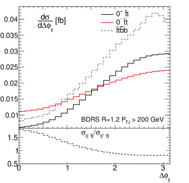
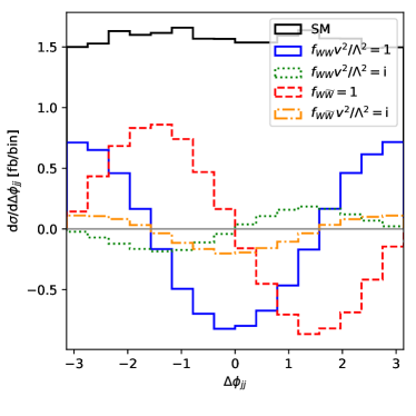
The situation is different for the Higgs-gauge Lagrangian, where -violation only occurs at dimension six. The general effective theory framework describing Higgs physics at the LHC is introduced in Sec. 7. In the effective Higgs-gauge Lagrangian, -odd couplings are described by the operators
| (A.104) |
With the Levi-Civita tensor, these operators are -conserving, -violating and -violating. The hard process which will allow us to determine the -properties of the gauge-Higgs interactions needs to include the or coupling. As illustrated in Fig. 16, this points to WBF Higgs production, associated production, or decays. The leading observable to test -violation is the one -odd and -odd observable constructed with the help of the Levi-Civita tensor. For the three different hard processes it corresponds to the signed azimuthal angle between the WBF tagging jets, the azimuthal angle between the leptons from the -decay, or the decay plane correlations in the Higgs decays. In the right panel of Fig. 17 we show the distribution of the signed azimuthal angle between the WBF tagging jets for different Wilson coefficients defined in Eq.(A.104). The interference with the SM rate is indeed anti-symmetric for the -odd coupling. Imaginary Wilson-like coefficients are not part of a consistent EFT prescription, but they can be used to illustrate the effect of re-scattering.
When we use appropriate kinematic distributions to search for effects from the specific -odd operators given in Eq.(A.104), the performance of angular correlations can be enhanced by including momenta in the -observables. The reason is that the dimension-6 operators have a new Lorentz structure, which comes with powers of 4-momenta in the Feynman rules. In Fig. 18 we show a comparison of the reach of the three leading signatures for -violation in the Higgs-gauge sector. The corresponding Feynman diagrams are shown in Fig. 16. The reach in terms of the new physics scale is shown on the right axis; it is computed using the Fisher information and information geometry Brehmer et al. (2017, 2018a). For each channel we compute the information available from the full phase space after basic acceptance cuts, from a combination of momentum-sensitive and -sensitive observables, and from the (optimal) -sensitive observable. For WBF Higgs production the latter is defined as an asymmetry in the signed azimuthal angle between the tagging jets,
| (A.105) |
For the other two channels, we use the appropriate combination of final state momenta instead. While WBF Higgs production and production indicate a similar reach, the Higgs decay channels are clearly less powerful.
Once we have convinced ourselves through these dedicated measurements that is not a good symmetry of the gauge-Higgs sector, the operators in Eq.(A.104) need to be included in global Higgs analyses described in Sec. 7 and Sec. 6.
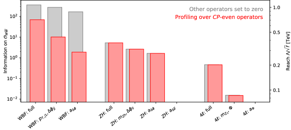
Figure from Ref. Brehmer et al. (2018a).
7 Effective field theory
In the absence of any ideas guiding new physics searches in the Higgs sector, we need a flexible and theoretically sound framework to describe and interpret precision Higgs studies. The goal of such a data-driven framework is to parameterize experimental limits on physics beyond the Standard Model — always assuming that in the presence of convincing anomalies we will aim for an interpretation in terms of fundamental physics models.
7.1 Coupling modifications
Historically Zeppenfeld et al. (2000); Duhrssen et al. (2004); Lafaye et al. (2009), indirect new physics effects on the couplings of the SM-like Higgs boson are parameterized as simple coupling modifiers
| (A.106) |
Analyses of this kind appeared soon after the Higgs discovery Klute et al. (2012); Plehn and Rauch (2012); Belanger et al. (2013); Giardino et al. (2014); Bechtle et al. (2014); Cheung et al. (2014). Modifications of the tree-level couplings appearing in the Standard Model loops are encoded into while extra possible new physics contributions are included as . In general, the loop-induced couplings have a non-trivial momentum dependence; for the Higgs couplings measurement we assume that all three external momenta are fixed, reducing the coupling to a single number. In terms of a Lagrangian we can write this hypothesis as Corbett et al. (2015a)
| (A.107) |
where
| (A.108) |
This Lagrangian is based on all SM-like structures at mass dimension four, but with shifts in the numerical values of the Higgs couplings. These modified couplings obviously affect all loop-induced Higgs couplings. In addition, it includes new higher-dimensional operators coupling the Higgs to photons and gluons. They arise from potential new particles in the loop and are normalized to their Standard Model values and . In the limit of heavy top masses these normalization constants read . In principle, we could include a more complete and gauge-invariant set of these kind of operators, but in all other cases they would compete with finite tree-level values and are phenomenologically less relevant. An alternative notation for the same framework is Duhrssen et al. (2004)
| (A.109) |
The same way that the modified couplings approach is only valid for SM-like couplings, , we have to ensure . Moreover, unlike the unique description of Eq.(A.106), in the -framework there exist several ways to treat modified loop-induced couplings which have to specified case by case. A possible Higgs decay to invisible states can be described by a wide variety of Lagrangian terms, but the experimental results are most easily quoted in terms of an invisible branching ratio.
The immediate benefit of the coupling modifications framework is that it defines a way to combine many Higgs rate measurements with a wide variety of initial states and final states. An open question is the treatment of the Higgs width.
First, we can keep the width as a free parameter. For illustration purpose, we assume that all Higgs couplings scale universally with . If we allow for an unobserved contribution to the total Higgs width the observable LHC rates then scale like
| (A.110) |
This relation defines a non-trivial scaling of the Higgs rates with the modified couplings in the presence of additional decay modes.
Alternatively, we can use the sum of the partial width from the observed Higgs channels as a lower limit on the physical Higgs widths,
| (A.111) |
One practical problem with this approach is that the charm Yukawa coupling is not small on the scale of the precision of the different LHC measurements. Given that to date the LHC has no sensitivity to this parameter in its SM range, we can use a flavor symmetry to identify . Higgs couplings to the light quarks are strongly constrained by the inclusive Higgs production rate, because they lead to tree-level production . Obviously, so-called invisible Higgs decays are perfectly measurable and contribute to Eq.(A.110).
An upper limit on the Higgs width comes from the unitarity constraints on scattering. For this process, the Standard Model value of the coupling saturates the unitarity limit. A new physics contribution to this coupling should therefore drive it away from the SM value, . Inside the Higgs coupling analysis this defines an upper limit on the Higgs width.
In practice, many global Higgs analyses promote Eq.(A.111) to a definition of the Higgs width. This implies that we assume that, up to small corrections, we have observed all relevant Higgs couplings with the corresponding production and decay processes.
In spite of its great success during the LHC Run I, this framework has three distinct problems:
-
1.
It is not renormalizable, which means that we cannot include electroweak precision predictions;
-
2.
It only describes modifications of total rates and cannot be used to interpret kinematic distributions;
-
3.
It does not allow us to combine Higgs measurements with other precision measurements.
7.2 Linear realization
From flavor physics we know how to describe effects from heavy particles on SM-like observables using effective field theory Buchmuller and Wyler (1986); Grzadkowski et al. (2010). In this framework a Lagrangian is defined by its particle content and its symmetries. The expansion parameter is the dimensionality of the individual operators, or inverse powers of a large matching scale. For example, we can construct a -symmetric Higgs Lagrangian including the usual Higgs-Goldstone doublet defined in Eq.(A.2). Truncated to dimension six the corresponding Lagrangian has the general form Hagiwara et al. (1993a); Grzadkowski et al. (2010)
| (A.112) |
where is the scale of the assumed UV complete model. It is constructed to be invariant under the full gauge symmetry of the Standard Model, but is not fully renormalizable or unitary. Obviously, we can extend this approach to the full SM Lagrangian, defining the general Standard Model Effective Field Theory (SMEFT) Gonzalez-Garcia (1999); Contino et al. (2013); Englert et al. (2014); de Blas et al. (2018)222For a comprehensive review of effective field theories of the Higgs sector we recommend Ref. Brivio and Trott (2017).. Obviously, the full set of SMEFT operators is constrained by a huge number of measurements. Therefore, the question becomes which of these operators affect Higgs observables at the LHC and which of them are not already constrained at a level that we can neglect their impact on LHC measurements. As the Run-II measurements become more precise, it becomes necessary to include increasing numbers of operators in the fits. The power of the SMEFT is that interdependent constraints arise from precision EW measurements, from di-boson production, and from Higgs production and decay. The current level of precision requires the inclusion of not only bosonic operators contributing to Higgs and gauge boson interactions, but also with fermion operators modifying the coupling of the and to the fermions when analyzing Higgs properties.
The minimum independent set of dimension-6 operators with the SM particle content (including the Higgs boson as an doublet) and compatible with the SM gauge symmetries as well as baryon number conservation contains 59 operators, up to flavor and Hermitian conjugation Grzadkowski et al. (2010). We start by imposing and invariance and employing for the bosonic sector the classical non-minimal set of dimension-6 operators in the Hagiwara-Ishihara-Szalapski-Zeppenfeld conventions Hagiwara et al. (1993a). In this case, the operators contributing to the Higgs interactions with gauge bosons are
| (A.113) | ||||||||
The Higgs doublet covariant derivative is , the hatted field strengths are and . The and gauge couplings are and . The operator contributes to the Higgs self-coupling and does not contribute to single Higgs production at tree level, while can be eliminated using the equations of motion.
In the gauge-Higgs sector, the basis operators important for Higgs fits are
| (A.114) |
They give rise to a variety of dimension-5 Higgs interactions with SM gauge boson pairs Hagiwara et al. (1993b),
| (A.115) |
with the usual field strengths. In this form we see that there are two classes of higher-dimensional operators, those leading to effects scaling with and those leading to effects scaling with . While the former can be constrained by total rate measurements, the latter describe modifications of kinematic distributions, like for example transverse momenta.
The effective couplings are related to the Wilson coefficients from Eq.(A.114) through
| (A.116) |
and
| (A.117) |
Gauge boson couplings from spontaneous symmetry breaking, just as Yukawa couplings, violate the Appelquist–Carazzone decoupling theorem Appelquist and Carazzone (1975). This means that the Higgs couplings to photons and gluons are suppressed by . New physics generally gives rise to dimension-6 operators suppressed by , leading to Higgs coupling strengths to photons and gluons scaling like .
Some of the above Higgs operators are strongly constrained by the electroweak precision data discussed in Sec. 2. For example, two gauge-Higgs operators contribute to the oblique parameters as
| (A.118) |
Even a generous limit of the order can be translated into a new physics scale TeV for , considerably smaller than what we can expect from the Higgs analysis. In specific UV complete models, the are generated with some specific scaling. Assuming corresponds to the assumption that the high scale physics is weakly interacting. In Ref. Arzt et al. (1995), the EFT operators are classified as operators that can be generated at tree level (and hence 1), and operators that are generated at loop level (). Alternatively, in models where the effective theory results from high-scale strong interactions, such as the SILH model Giudice et al. (2007), the scaling of the depends on the strong coupling and heavy resonance scale.
There are many ways to expand this set of operators to a complete basis. We follow Ref. Corbett et al. (2012). Other basis choices include the general Warsaw basis Grzadkowski et al. (2010) or the model-inspired SILH set Giudice et al. (2007). Translations between actual bases are simple linear transformations Falkowski et al. (2015).
For the Higgs interactions with fermion pairs Grzadkowski et al. (2010) the problem is a lack of appropriate observables in the LHC Higgs measurements. This allows us to limit the analysis to the flavor-diagonal Yukawa structures
| (A.119) |
with . The corresponding effective Lagrangian reads
| (A.120) |
The operator leads to a finite renormalization of the Higgs field and hence a universal shift of all Higgs couplings to Standard Model fields. In analogy to the Higgs-gluon coupling we scale the fermionic Wilson coefficients by a factor to reflect the chiral nature of the Higgs coupling operators. In terms of the physical Higgs field we find
| (A.121) |
where for we define the physical masses and fermions in the mass basis.
Comparing Eq.(A.115) and Eq.(A.121) to Eq.(A.106) we see that the SMEFT framework for the Higgs sector is closely related to the coupling modifiers. All modified Higgs couplings are present in the SMEFT description; the only caveat is that the SMEFT Lagrangian at dimension six features custodial symmetry, translating into the hard-wired condition . This is, if anything, a shortcoming of the SMEFT approach and a reason to think about including dimension-8 operators. In addition to the six independent coupling modifiers , the SMEFT Lagrangian features new Lorentz structures linked to and as well as modifications of the still unmeasured interaction.
A key feature of the effective Higgs-gauge Lagrangian in Eq.(A.114) is that it also leads to deviations of the triple-gauge couplings Falkowski et al. (2016, 2017); Berthier et al. (2016); de Blas et al. (2018); Liu and Wang (2018). This means that pair production of electroweak bosons at the LHC has to be combined with the global Higgs EFT analysis. The one additional purely bosonic operator describing the process at the LHC is Butter et al. (2016b)
| (A.122) |
The combined operators from Eq.(A.113) and Eq.(A.122) are related to the historic notation for anomalous gauge couplings Gaemers and Gounaris (1979),
| (A.123) |
with , , , , and . Equations (A.123) and (A.124) use for the modification of the vertex since this is standard notation, while in the remainder of this work always refers to Higgs couplings. The gauge-invariant form of the anomalous gauge couplings at mass dimension six reads (see also de Blas et al. (2018) for a detailed comparison)
| (A.124) |
Of the five modified triple gauge couplings only three are independent when written in terms of an effective gauge theory. This linear relation reflects the fact the the traditional variables are nothing by a gauge-dependent re-parametrization of the Wilson coefficients of the SMEFT. Using anomalous couplings for an analysis does not improve any shortcomings of a SMEFT analysis, it only removes weak gauge invariance from the list of assumptions.
Finally, we have to account for the fact that di-boson observables at the LHC are also affected by fermionic operators of the form
| (A.125) |
with the generators . The quark doublet can be replaced by the lepton doublet or, for the singlet case, by right-handed fermions. Because of the hermitian structure of the Lagrangian, these operators do not actually contribute to any Higgs couplings, but they do contribute to anomalous weak gauge couplings. To simplify the analysis, we can for instance assume that the fermion operators are generation universal Alves et al. (2018), which allows us to remove the operators coupling to lepton doublets. In addition, at the expected level of accuracy in the Higgs-gauge fit we can neglect all operators with a non-trivial flavor structure. While anomalous gauge boson couplings to light fermions are constrained by electroweak precision data Franceschini et al. (2018), they have to be included in an LHC analysis unless we have a firm reason to expect a hierarchy of scales between LEP and LHC limits Baglio et al. (2017, 2018); Ellis et al. (2018); Alves et al. (2018). In that case an additional set of terms in the effective Lagrangian becomes
| (A.126) |
where we ignore the contribution to the Fermi constant from 4-lepton interactions. Note that eventually the Higgs-gauge analysis in the SMEFT framework also has to be combined with the top sector, for more information we refer to the TopFitter analyses Buckley et al. (2015, 2016).
7.3 Non-linear realization
An alternative effective Lagrangian of the Higgs sector is based on a non-linear realization of electroweak symmetry breaking (HEFT) Alonso et al. (2013); Brivio et al. (2014a); Buchalla et al. (2014a, b); Gavela et al. (2014); Brivio et al. (2014b). Here, the Higgs is not embedded in a doublet together with the Goldstone modes, as motivated by the symmetry structure of certain UV completions. We can nevertheless link the non-linear and linear operator sets in terms of canonical dimensions. This connection is usually established through the ratio of scales , where can be related to the scale of strong dynamics. A detailed analysis of the non-linear model reveals a double ordering: first, there is the chiral expansion, and in addition there is the classification in powers of . Following Refs. Buchalla et al. (2016); Corbett et al. (2015b); Brivio et al. (2016), a subset of the non-linear Lagrangian can be linked to the -framework of Eq.(A.107), with the additional assumption Klute et al. (2012). As for the linear representation, an extended set of non-linear operators provides a natural extension to include kinematic distributions at the LHC and can be used for global LHC analyses de Blas et al. (2018).
To illustrate the link between the linear and non-linear effective Lagrangians we start with the reduced bosonic -even operator set of order Brivio et al. (2014a),
| (A.127) | ||||||||
and
| (A.128) | ||||||||
where and are the vector and scalar chiral fields in the adjoint representation of . The unitary matrix contains the Goldstone modes () , , and transforms as a bi-doublet under the global transformations. The covariant derivatives act on the fields as Brivio et al. (2014a)
| (5) |
The functions are power series of the Higgs singlet field and introduce the anomalous Higgs couplings. For the Higgs analysis at the LHC we truncate their expansion after their linear term in . A link of single Higgs rates to Higgs pair production, as provided in the SMEFT approach, is not possible in the non-linear HEFT setup.
This number of operators can be reduced for an LHC analysis. First, operators containing the combination are irrelevant for on-shell gauge bosons or when the fermion masses in the process are neglected. This removes and for the Higgs analysis. While and , together with and , will eventually help us to distinguish linear from non-linear electroweak symmetry breaking Brivio et al. (2014a), they do not affect three-point Higgs couplings. For the same reason we can also omit and . For on-shell Higgs amplitudes and lead to coupling shifts Brivio et al. (2014b), i.e. their effect can be accounted for by a re-definition of the remaining non-linear operator coefficients. Finally, for illustration purpose we neglect and , because of their contributions to the electroweak oblique parameters.
Again in analogy to the linear ansatz of Eq.(A.120) we add three Yukawa-like non-linear operators of the type
| (A.129) |
Given this simplified fermion sector we can absorb a combination of and through the equations of motion and arrive at a 9-dimensional non-linear operator set. If we use a particularly simple form for the Wilson coefficients
| (A.130) |
we can link the non-linear Lagrangian and the linear Lagrangian relevant for our Higgs analysis,
| (A.131) |
While the link between the non-linear effective Lagrangian to the -framework is well known, there also exists a one-to-one correspondence between the linear and a non-linear operator set. The LHC results in the two approaches can be translated into each other through a simple operator rotation. However, these relations are valid only when we study the effects of the operators restricted to Higgs interactions with two SM fields and do not include anomalous gauge boson couplings. The link between anomalous Higgs couplings and triple gauge couplings in the SMEFT approach does not have any correspondence in the HEFT.
7.4 Decoupling the 2HDM
To illustrate the link between the effective field theory and for example the extended Higgs sectors introduced in Sec. 5 we show how the 2HDM with a large mass hierarchy can be matched to the effective theory. Per se it not clear if this matching should be performed in the unbroken or broken phase, i.e. including terms of the order or setting . This choice is particularly relevant because the decoupling theorem does not hold in the presence of a vacuum expectation value, which implies that terms proportional to do not have to decouple with the new heavy particles. For simplicity we assume that all additional Higgs bosons are heavy,
| (A.132) |
To construct the effective theory Gunion and Haber (2005); Randall (2008) we start from the relations between the Higgs self-couplings, masses and mixing angles in the decoupled regime
| (A.133) |
In terms of the combination
| (A.134) |
we can define a convenient decoupling parameter related to the scale separation as
| (A.135) |
If the effective field theory description of the 2HDM approaches the decoupling limit , the expansion parameter scales like , requiring The correlation of the mixing angles is a key property of the hierarchical 2HDM. For sufficiently large this gives for the expansion parameter
| (A.136) |
We can now expand all modifications of the light Higgs couplings given in Tab. 3 in terms of . We show the complete list of coupling modifications in Tab. (7). The main feature is that the gauge couplings in the 2HDM decouple significantly faster than the Yukawa couplings, especially the down-type Yukawa couplings with their enhancement.
In addition to the tree-level mixing effects, the heavy charged Higgs states also contribute to the effective Higgs-photon interaction. To compute it, we need to consistently expand the corresponding trilinear Higgs coupling,
| (A.137) |
Note that this coupling, like all triple Higgs couplings, does not decouple. The proper mass dimension of the Wilson coefficients of is ensured by the heavy particles in the loop, as illustrated in e.g. Eq.(A.35).
B Experimental results
1 Gluon Fusion
The dominant production mechanism for the Higgs boson in hadronic collisions is the gluon fusion process shown in Fig. 19,
| (B.1) |
The gluon fusion production mode was the driving force behind the Higgs discovery in 2012, Fig. 1, subsequent Higgs mass measurements, Fig. 13, and most measurements of Higgs couplings so far. Due to the loop-induced gluon-Higgs coupling discussed in Sec. 3, gluon fusion not only enables high-precision measurements of the total production rate, it also offers unique opportunities for coupling measurements from its kinematic distributions.

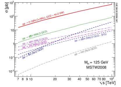
1.1 Motivation and signature
Gluon fusion, with the subsequent decays
| (B.2) |
is one of the most important channels for Higgs studies and as seen in Fig. 19, the gluon fusion rate is significantly larger than that of the other channels. Due to overwhelming QCD backgrounds and the lack of additional signatures to tag or trigger on, is not accessible. Given the plethora of Higgs final states that can be accessed through gluon fusion, this process sits at the heart of the LHC Higgs phenomenology program.
In particular the observation of Higgs decay to a photon pair and a leptonically decaying -boson pair is a tell-tale indication of the Higgs interactions and electroweak symmetry breaking. On the one hand, as the photons do not have a mass, the decay of the Higgs to photons is loop-suppressed and therefore sensitive to the interplay of the gauge-Higgs and fermion-Higgs sectors. In the Standard Model there is a delicate interference between the charged and top loops as detailed in Sec. 3.4. In particular the fermion-Higgs interactions in new physics models can be vastly different from the Standard Model, as indicated by the well-motivated two-Higgs doublet models. The observation of at close to the predicted rate is therefore a strong validation of the Standard Model.
Phenomenologically, searches for amount to hunting for bumps on top of a continuously falling di-photon distribution, as illustrated in Fig. 1. Photons are experimentally well-understood, including the fact that most jets consist of photons due to the anomaly-mediated decay, and care has to be taken to understand this background. In practice, the combined background is estimated in a data-driven approach through fitting polynomials. This way, even though the decay only happens at the 2 per-mille level, the impact of systematic uncertainties is relatively small and the Higgs boson could be observed at a statistically significant level already early on in the LHC program.
On the other hand, the decays and highlight the Higgs couplings to the massive weak bosons and their longitudinal degrees of freedom. Such an interaction is a direct implication of the Higgs mechanism itself. The decay is typically observed in fully leptonic final states which are experimentally clean and lead to a clear resonance peak at . Again, electrons and muons are well-understood objects in the ATLAS and CMS detectors, and the final state can be reconstructed without systematic limitations and with small irreducible backgrounds. Compared to the case, is statistically limited through the leptonic branching ratios, which significantly reduces the naive branching ratio of 2.6% in the Standard Model. The decays and require special attention to the involved hadronic or missing energy signatures and are in general more complicated to reconstruct.
1.2 Precision prediction
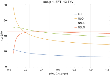
| 7 TeV | 16.87 pb | |||
| 8 TeV | 21.45 pb | |||
| 13 TeV | 48.68 pb | |||
| 14 TeV | 54.80 pb | |||
| 28 TeV | 154.63 pb | |||
| 100 TeV | 808.23 pb |
Since the extraction of Higgs properties often relies on normalizing the rate to the SM predictions, an extraordinary effort has been made to obtain the most precise theoretical predictions.
The primary contribution to gluon fusion is through the couplings to heavy fermions, , which is shown in Fig. 19. This process is dominated by the contributions of the top quark loop and the loop with a bottom quark contributes roughly to the SM cross section. The QCD corrections to the rate are large and known to N3LO order in the heavy-top limit, and they increase the rate from the LO prediction by more than a factor of 2, as seen in Fig. 20. The significant reduction in the scale dependence at higher orders is clear. Historically, the gluon fusion rate was computed in the large top mass limit. In the heavy quark limit, the lowest order partonic cross section is independent of the top quark mass and becomes a constant for infinite top quark mass,
| (B.3) |
Heavy chiral fermions whose masses arise from couplings to the Higgs field’s vacuum expectation value do not decouple at high energy and the gluon fusion rate essentially counts the number of SM-like chiral quarks. Hence, the observation of a Higgs production rate consistent with the SM expectation (e.g. in the decay to bosons) immediately rules out the possibility of a generation of SM-like chiral fermions Kribs et al. (2007); Denner et al. (2012a); Anastasiou et al. (2011).
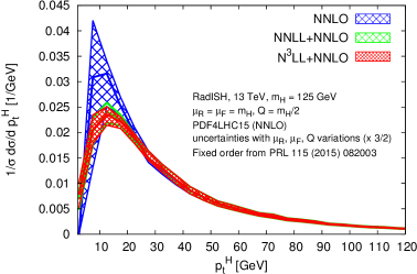
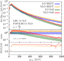
The NLO Dawson (1991); Graudenz et al. (1993); Djouadi et al. (1991), NNLO Harlander and Kilgore (2002); Anastasiou and Melnikov (2002); Ravindran et al. (2003), and N3LO Anastasiou et al. (2015a, 2014, b); Mistlberger (2018); Cieri et al. (2018) results are known in the limit, while the NLO results Graudenz et al. (1993); Spira et al. (1995) are known analytically with the full top quark mass dependence. Fig. 20 illustrates the convergence of the QCD expansion and the reduction of scale dependence at higher orders. The effects of a finite top mass can be included to NNLO Harlander and Ozeren (2009a); Pak et al. (2010); Harlander and Ozeren (2009b) numerically as an expansion in , while N3LO results are available for Anastasiou et al. (2016). Electroweak corrections are known to NLO Aglietti et al. (2004); Actis et al. (2008, 2009) and mixed QCD/electroweak corrections Anastasiou et al. (2009); Bonetti et al. (2018a, b) are partially known. The electroweak corrections increase the rate by . The fixed order rates along with estimated uncertainties have been computed by the LHC Higgs Cross Section Working group de Florian et al. (2016a), with fixed order results shown in Tab. 8. The gluon fusion rate increases significantly with beam energy, as demonstrated in Fig. 19. This figure includes most known higher order corrections and the widths of the curves represent an estimate of the uncertainties. The differential rate is known at NNLO Dulat et al. (2018, 2017).
The NNLO rate can be further improved by the resummation of threshold effects from soft, virtual, and collinear gluons Kramer et al. (1998). These contributions to the total gluon fusion rate are known at N3LL Bonvini and Marzani (2014). Comparison of a combined threshold and high energy resummation with the fixed order N3LO result shows that the resummation effects are small at this order Bonvini et al. (2016); Bonvini and Marzani (2018).
As we will discuss in Sec. 1.4, the kinematics of Higgs production in gluon fusion can be used to search for new physics effects. At LO, the Higgs boson has no and a transverse momentum spectrum for the Higgs is first generated by the process , as well as (anti)quark scattering . The Higgs transverse momentum is shown on the left of Fig. 21. The total rate for Higgs plus jet production receives corrections from the contributions of the quark. Fixed order NLO and NNLO Glosser and Schmidt (2002); Boughezal et al. (2013, 2015a, 2015b); Dulat et al. (2018); Chen et al. (2015b); de Florian et al. (1999) radiative corrections to the Higgs plus jet rate are known for infinite top quark mass and the NLO rate with full top quark mass dependence is now available Lindert et al. (2018); Jones et al. (2018); Neumann (2018). In Fig. 21 we see how for the top loop can be resolved. The Higgs plus jet processes are part of the NLO (real emission) contribution to the gluon fusion process Ellis et al. (1988), which break the LO color correlation of the initial state as required by the color singlet Higgs at LO. The large radiative corrections to the Higgs plus jet spectrum can therefore be understood in terms of kinematically un-suppressed QCD emission of the initial state in the presence of a large effective color charge of the gluon (the Casimir of the adjoint representation of is ), rather than a breakdown of perturbation theory. Integrating over the QCD radiation in the NNLO gluon fusion calculation yields an NNLO prediction for the Higgs spectrum. The fully differential Higgs production rate to NNLO is implemented in the codes FEHip Anastasiou et al. (2004, 2005) and Hnnlo Catani and Grazzini (2007); Grazzini (2008). The NNLL resummation Bozzi et al. (2006); de Florian et al. (2011); Cao et al. (2009) of the small and also the N3LL Chen et al. (2016); Bizon et al. (2018) contributions are known and both the fixed order and matched results are shown in Fig. 21. The resummation significantly reduces the peak of the spectrum relative to the fixed order prediction.
The backgrounds to the different Higgs decays is very different depending on how many jets are accompanying the Higgs. This is particularly evident in the decay , where in the -jet bin the dominant background is from continuum production, while the - and - jet bins have large backgrounds from top quark pair production Stewart and Tackmann (2012). To minimize the background, the experiments split the signal into different jet multiplicity bins which introduces a scale, and hence large logarithms of the form . Resumming these logarithms and estimating the uncertainty from the separation of scales introduces a significant theoretical uncertainty.
1.3 LHC analyses
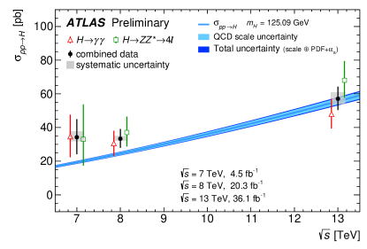
The measured Higgs total cross section from ATLAS (in the and channels) is shown in Fig. 22 and can be seen to be in reasonable, but not perfect, agreement with theory. At 13 TeV, the Higgs has been well-established in the channels, Fig. 23. Arguably the cleanest signature of gluon fusion is , see collaboration (2018a); Sirunyan et al. (2018a), which gives
| (B.4) |
for the ATLAS result which is based on the large luminosity of . The region selected by this analysis, , has an expected cross section times branching ratio of , and the experimental result therefore agrees well with the prediction, corresponding to
| (B.5) |
The latest CMS result is based on and measures
| (B.6) |
for a theoretically expected fiducial cross section of fb. Again this is in good agreement with the theory. Turning to less inclusive measurements, we show the jet- spectrum in gluon fusion events in the right-hand side of Fig. 23. As can be seen, the high-precision predictions detailed above are required to model the transverse momentum spectrum satisfactorily given that gluon fusion provides the largest contribution to the Higgs spectrum. The sensitivity of gluon fusion to the top quark threshold which effectively embeds top quark scattering for center-of-mass energies larger than has motivated a range of interesting and BSM-relevant analyses. Most of our understanding of the Higgs boson that was summarized in Sec. 6.1 is based on gluon fusion production, and we will discuss BSM-specific implications of gluon fusion kinematics in the next section 1.4. There we will comment on how the measurements of the Higgs boson’s kinematic properties in the gluon fusion process, which are already under good control (see Fig. 23 right), can be used to obtain a detailed picture of the Higgs boson interaction modifications in non-resonant BSM extensions.
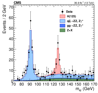
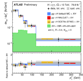
The gluon fusion channel can be used to obtain limits on the new resonant physics, including heavy pseudoscalars present in the 2HDM, MSSM, and NMSSM, through the process,
| (B.7) |
where can be the SM Higgs Boson or one of the heavier neutral scalars present in these models. Searches have been made for and and also . The exclusions are model dependent. Given the well-understood phenomenology of these scenarios, searches often draw from the specific correlations of different production and decay modes. We will therefore focus on these scenarios in more detail in Sec. 6.2.
1.4 Power of kinematics
If we take the definition of the gluon fusion process in Eq.(B.1) seriously, it represents much more than a total rate measurement. Two obvious signatures are off-shell Higgs production, as discussed in Sec. 6, and boosted Higgs production recoiling against one or more hard jets illustrated in Fig. 21. Both of these processes allow us to move beyond the heavy-top limit in the gluon-Higgs coupling discussed in Sec. 3 and probe the structure of the corresponding loop(s). A simple theory hypothesis based on the dimension-6 SMEFT Lagrangian combines the top Yukawa coupling with the effective Higgs coupling to gluons Banfi et al. (2014); Azatov and Paul (2014); Grojean et al. (2014); Buschmann et al. (2015),
| (B.8) |
where is defined In Eq.(A.31) and is the limit. It is obvious from Eq.(B.8) that gluon fusion alone cannot distinguish between and . Note that for these terms the modified Higgs couplings from Sec. 7.1 and the linearly realized SMEFT from Sec. 7.2 are equivalent. In terms of physics beyond the Standard Model we assume that a new particle generates a finite , but without altering the kinematic structure of the coupling. The appearance of the modified top Yukawa coupling indicates that an alternative way to search for the same scenario includes production, discussed in Sec. 4.
(80,50) \fmfsetarrow_len2mm \fmfleftg1,g2 \fmfrighth1 \fmftopg3 \fmflabelg1 \fmflabelg2 \fmflabelg3 \fmflabelh1 \fmfgluon,width=0.6v1,g1 \fmfgluon,width=0.6g2,v2 \fmffermion,tension=.05,width=0.6v1,v2 \fmffermion,tension=.8,width=0.6v2,v3 \fmffermion,tension=.8,width=0.6v3,v1 \fmfdashes,width=0.6v3,h1 \fmffreeze\fmfphantom,tension=100,width=0.6g2,v4 \fmfphantom,tension=100,width=0.6v4,v2 \fmfgluon,width=0.6v4,g3 {fmfgraph*}(100,60) \fmfsetarrow_len2mm \fmfleftg1,g2 \fmfrightZ1,Z2 \fmflabelg1 \fmflabelg2 \fmflabelZ1 \fmflabelZ2 \fmfgluon,width=0.6v1,g1 \fmfgluon,width=0.6g2,v2 \fmffermion,tension=0.35,width=0.6v1,v2 \fmffermion,tension=0.7,width=0.6v2,v3 \fmffermion,tension=0.7,width=0.6v4,v1 \fmffermion,tension=0.35,width=0.6v3,v4 \fmfgluon,width=0.6v3,Z2 \fmfdashes,width=0.6v4,Z1 {fmfgraph*}(100,60) \fmfsetarrow_len2mm \fmfleftg1,g2 \fmfrightZ1,Z2 \fmflabelg1 \fmflabelg2 \fmflabelZ1 \fmflabelZ2 \fmfgluon,width=0.6,label.side=leftg1,v1 \fmfgluon,width=0.6g2,v2 \fmffermion,tension=.05,label=,label.side=left,width=0.6v1,v2 \fmffermion,tension=.8,width=0.6v2,v3 \fmffermion,tension=.8,width=0.6v3,v1 \fmfdashes,tension=1.5,width=0.6,label=,label.side=rightv3,v4 \fmfphoton,tension=0.8,width=0.6v4,Z1 \fmfphoton,tension=0.8,width=0.6v4,Z2 \fmffreeze\fmfphantom,tension=0.8,width=0.6,label=,label.side=right,label.dist=2.5v4,v2 {fmfgraph*}(100,60) \fmfsetarrow_len2mm \fmfleftg1,g2 \fmfrightZ1,Z2 \fmflabelg1 \fmflabelg2 \fmflabelZ1 \fmflabelZ2 \fmfgluon,width=0.6,label.side=leftg1,v1 \fmfgluon,width=0.6g2,v1 \fmfvlabel.side=right,label.dist=15,label=v1 \fmfvdecor.shape=circle,decor.filled=shaded,decor.size=15v1 \fmfdashes,tension=1.5,width=0.6,label=v1,v4 \fmfphoton,tension=0.8,width=0.6v4,Z1 \fmfphoton,tension=0.8,width=0.6v4,Z2
As a starting point, we note that we could search for absorptive threshold contributions in the kinematics of Higgs plus jets production shown in Fig. 24. However, those effects are too small to give us access to and Buschmann et al. (2014). Alternatively, we search for top mass effects in the spectra of the outgoing Higgs and one Baur and Glover (1990a); Banfi et al. (2014); Grojean et al. (2014); Schlaffer et al. (2014) or more Buschmann et al. (2014); Greiner et al. (2017) jets
| (B.9) |
In the left panel of Fig. 25 we show the corresponding change in the slope above the top mass. For a benchmark point we need to ensure that the inclusive Higgs production rate is not significantly changed, as for example for . Based on an optimistic 2-dimensional likelihood analysis we can estimate the impact of the -distribution as ruling out this benchmark point at 95% C.L. with an integrated luminosity of of 13 TeV LHC data.
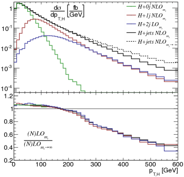
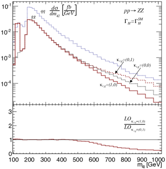
A second way to test exactly the same physics hypothesis is off-shell Higgs production. In this case, the change in the momentum dependence of the Higgs-gluon coupling will appear through the interplay of the signal Feynman diagrams shown in Fig. 24. At large we can approximate the external gauge bosons with their Goldstone modes and we can understand the signal amplitude in terms of its longitudinal components Glover and van der Bij (1989); Azatov et al. (2015a); Cacciapaglia et al. (2014)
| (B.10) |
with defined in Eq.(A.32) and we consider the purely leptonic decay channel, . In the low-energy limit , it reproduces the usual effective Higgs–gluon coupling. However for this measurement we are interested in the low-energy regime with
| (B.11) |
The logarithmic dependence on is similar to the boosted Higgs case. Eventually, the ultraviolet divergence cancels between the Higgs amplitude and the continuum. The relative sign between the full top mass dependence and the low-energy limit leads to a distinctive interference pattern with the continuum, where the top mass dependence predicts a destructive interference. We show this effect in the right panel of Fig. 25. Again, an optimistic 2-dimensional likelihood analysis in terms of and the leading angular correlation indicates that we can rule out the benchmark point at 95% C.L. with an integrated luminosity of of 13 TeV LHC data, significantly later than using the boosted Higgs signature.
A third, indirect way to test yet the same hypothesis is Higgs pair production Azatov et al. (2016), but due to the small rate we do not expect such a measurement to contribute significantly.
Finally, the elephant in the room is the direct rate measurement. As we will see in Secs. 4 and 6, production, together with the measurement of the Higgs production rate in gluon fusion, will likely lead to the best reach. On the other hand, while these specific kinematic regions appear less attractive to test a simple and well-defined hypothesis, they offer important consistency tests of our underlying hypotheses in a situation where we have to rely on appropriate measurements to identify BSM physics in the Higgs sector.
2 Weak boson fusion
Weak boson fusion (WBF),
| (B.12) |
is an especially attractive relevant Higgs production process for a multitude of theoretical and experimental reasons. As illustrated in Fig. 26 it directly probes gauge boson scattering and is therefore a sensitive probe of any physics that relates to perturbative unitarity conservation Lee et al. (1977b, a).
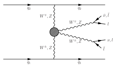
2.1 Motivation and signature
A key WBF signature from a theory perspective is based on the decay Cahn and Dawson (1984). In the high energy limit, gauge boson scattering () is described in terms of the longitudinal degrees of freedom, and the scalar matrix element has the simple form
| (B.13) |
where is the energy of the sub-process. Divergent scattering probabilities are only avoided through a cancellation of the , which are dimensionful constants including coupling constants and masses Lee et al. (1977b). In the Standard Model the relevant couplings are
| (B.14) |
The contributing quartic and trilinear couplings are , , and . This way is protected by gauge invariance. The second sum rule is sensitive to the custodial isospin relation and the Higgs coupling Birkedal et al. (2005); Englert et al. (2015b). These cancellations are indeed tantamount to spontaneous symmetry breaking Cornwall et al. (1973, 1974), and although models with non-SM symmetry breaking realize unitarity cancellations in often non-trivial ways (for example in the case of Higgs triplets), in generic perturbative extensions of the Standard Model they remain intact. This motivates searches for new resonances linked to the Higgs sector in WBF production Birkedal et al. (2005); Frank et al. (2013); Englert et al. (2015b).
One could therefore imagine that physics which modifies the unitarity sum rules, e.g. through the value of , will also lead to large enhancements of the WBF production rate. The problem is that all four gauge bosons couple to light fermions, which means that longitudinal contributions are mass-suppressed and the unitarity sum rules are not directly accessible without high statistics. However, the tendency of (non-)perturbative models to enforce unitarity at least up to some intermediate scale with additional resonances still makes weak boson fusion a well-suited process to measure or constrain the presence of (non)-resonant new physics as thresholds are also visible for transverse polarizations (for which the high energy-limit is trivial) Englert et al. (2015b).
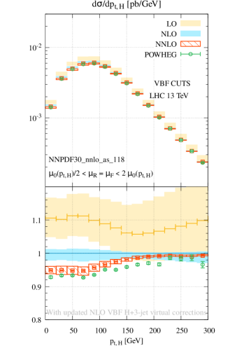
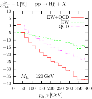
Experimentally, weak boson fusion processes have a distinct signature Kleiss and Stirling (1988); Baur and Glover (1990b); Barger et al. (1991a); Rainwater et al. (1996); Rainwater and Zeppenfeld (1999); Cox et al. (2011); Barger et al. (1989). To produce the Higgs, the incoming quarks are probed at large momentum fractions while the radiated weak bosons lead to a comparably small transverse momentum Dawson (1985). This leads to two energetic forward jets at large invariant mass, separated by a large rapidity gap. The Higgs is produced centrally and with sizeable transverse momentum, allowing us to search for the Higgs decays Rainwater et al. (1998); Plehn et al. (2000); Rainwater and Zeppenfeld (1999); Kauer et al. (2001); Eboli and Zeppenfeld (2000)
| (B.15) |
The absence of QCD radiation into the central region follows from the vanishing color factor when we exchange a gluon between the incoming quarks, and the tiny interference between the WBF -channel and -channel amplitudes. It allows us to use information on the central jet activity, to first order central jet vetos, as formidable tools to enhance the Higgs signal over the backgrounds Barger et al. (1991b, 1995); Bernaciak et al. (2014); Biekötter et al. (2017). This includes the irreducible gluon-fusion Higgs production that contributes around 15% to the Higgs production for typical WBF cuts that can be reduced to a few percent level as these processes are characterized by a central QCD emission profile Andersen et al. (2009, 2010).
Finally, an advantage of the WBF process over Higgs production in gluon fusion, is that the 3-particle final state allows us to study many aspects of the interaction. For example, the sensitivity to the properties of this vertex are discussed in Sec. 6.3. The WBF version of the off-shell Higgs measurement introduced in Sec. 6.1 is actually the more robust channel to constrain the Higgs width Englert et al. (2015a) when we fully correlate the production and decay and in this way minimize the vulnerability to unknown BSM loop contributions Englert and Spannowsky (2014); Campbell and Ellis (2015).
2.2 Precision predictions
The particular structure of the WBF topology from a QCD point of view as “double-deep inelastic scattering” also renders this process quite non-standard in terms of expected perturbative QCD corrections. QCD radiation into the central part of the detector is highly suppressed. Interference of the weak boson fusion contribution with associated Higgs production Ciccolini et al. (2008) or gluon fusion is negligible Bredenstein et al. (2008) for acceptance cuts that select the WBF signal region.
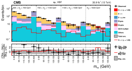
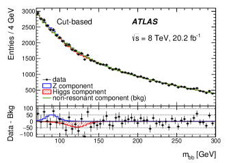
The dominant QCD emission effects are therefore related to bremsstrahlung in the direction of the quark legs. Due to the color singlet -channel exchange, there are no one-loop contributions that color-connect the external quark legs. The small NLO QCD corrections can be almost entirely absorbed into parton densities through choosing the factorization scales for the incoming partons as the -channel momentum transfer of the radiated weak boson, all in agreement with the deep inelastic scattering paradigm Jager et al. (2006a, b); Bozzi et al. (2007). Considering the next order in perturbation theory, the NNLO QCD corrections change the total cross section by around 5% Bolzoni et al. (2012); Cacciari et al. (2015); Cruz-Martinez et al. (2018), computed again in the structure function approximation that assumes no correlation between the incoming protons. In Fig. 27 we show the effects of the NNLO QCD corrections on the transverse momentum of the Higgs. The radiation of a second jet renders the transverse momentum spectrum slightly softer, especially around the maximum . As also shown in this plot, this kind of effect is expected from the parton shower treatment of the second jet radiation. Predictions for WBF production in association up to three jets have been discussed in Refs. Campanario et al. (2013, 2018).
Given the small QCD corrections, WBF Higgs production is one of the LHC processes where we also need to control the electroweak corrections. Similar to the NLO QCD corrections, the NLO electroweak corrections to the total WBF rate range around 5%. For the total cross section, the QCD and electroweak corrections largely cancel each other Ciccolini et al. (2007, 2008); Figy et al. (2012). In the right panel of Fig. 27 we show the effect of the electroweak corrections on the transverse momentum of the leading jet. While the QCD corrections switch sign around the maximum of the distribution, the electroweak corrections are always negative and increase towards larger momentum as expected for electroweak corrections leading to large Sudakov logarithms.
2.3 LHC Analyses
One of the Higgs signatures which relies on the WBF production channel is the decay to tau leptons Sirunyan et al. (2018b). The approximate reconstruction of the invariant mass only works when the decaying Higgs has sizeable transverse momentum. In the left panel of Fig. 28 we show the signal and backgrounds for leptonic decays of the -pair. The main background is +jets production, which can actually be divided into a QCD process with and an electroweak process with . The difference between them is that the latter has a color structure like the signal, so the analysis of the central jet activity only suppresses this background based on small kinematic differences. Typically, the combined +jets background is dominated by the QCD process before we take into account the central jet activity, while after including this information the two processes are of similar size. Increasing the cut on the tagging jets through reduces the size of the signal, but it leads to an even bigger improvement of . This shows how we can use the properties of the hard signal process to significantly reduce the backgrounds.
In the right panel of Fig. 28 we show an attempt to extract the Higgs decay in WBF. Given the pure QCD nature of the signal process, it is difficult to extract this process from the backgrounds. Therefore, available constraints are too weak to obtain limits on SM-like production, see Fig. 28. Proof-of-principle investigations, however, suggest that relying on advanced analysis strategies this channel will allow us to set constraints on the associated Higgs interactions Englert et al. (2016a). The channel discussed in Sec. 3 provides another avenue to test these couplings.
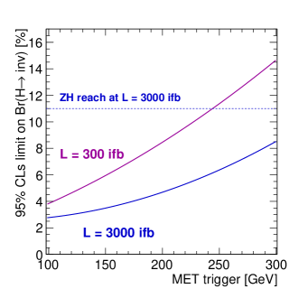
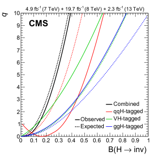
The WBF production process is the best way to search for invisible SM-like Higgs decays at the LHC Eboli and Zeppenfeld (2000); Bernaciak et al. (2015); Biekötter et al. (2017). In the left panel of Fig. 29 we compare the reach of this channel with the second-best strategy, based on production. While WBF has an advantage with its sizeable transverse momentum of the Higgs boson with a maximum around , triggering is a problem. We have to rely on a combination of missing transverse energy with two forward tagging jets. This problem can be solved by production combined with a leptonic -decay, as will be discussed in Sec. 3. Towards high LHC luminosities we see that the WBF analysis always wins over the channel, provided we can trigger on missing transverse momentum below around 300 GeV Biekötter et al. (2017). In the right panel of Fig. 29 we show the results of a CMS search for invisible Higgs decays using WBF production, production, and gluon fusion Higgs production including a hard jet. While the expected hierarchy of the channels is WBF ahead of ahead of gluon fusion, the observed limit is driven by production. Combining all analyses gives a 95% C.L. limit of , assuming all Higgs couplings to be SM-like. A more complete analysis, including variable Higgs couplings, will be the topic of Sec. 6. Such invisible Higgs decays can be interpreted in direct relation with dark matter, in particular through the Higgs potential role in portaling to a hidden sector through the SM singlet operator as outlined in Sec. 5.1. If additional dark fields are sufficiently light, the Higgs can obtain a new invisible decay channel that would manifest itself as an invisible branching ratio Butter et al. (2016a).
Finally, WBF production is also an important channel for new physics searches in visible final states. interactions can be large in the context of the Georgi-Machacek model where a hierarchy in triplet vs double-induced electroweak symmetry breaking can be relaxed Fig. 30. The presence of these vertices links to how unitarity is restored in such models as discussed above. Searches for doubly charged Higgs bosons proceed in a similar fashion. As the branching ratio of is enhanced for heavy doubly charged Higgs masses (completely analogous to the case of the SM decay ), clean same-sign lepton jet searches can be used to obtain more stringent constraints on triplet electroweak symmetry breaking, Fig. 30.
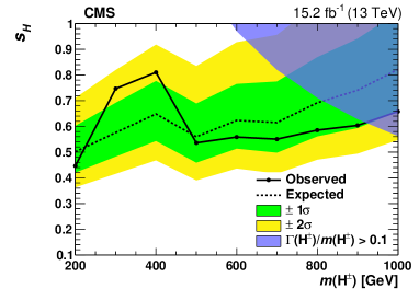
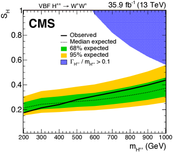
3 Associated production
Associated Higgs production with a weak boson, also called Higgs-strahlung,
| (B.16) |
corresponds to the working horse channel at LEP or at future electron-positron colliders. Unlike at lepton colliders, it is not the production channel with the leading cross section. As a matter of fact, it was clear from the very beginning that this channel would hardly contribute to a Higgs discovery.
On the other hand, production is the most experimentally clean Higgs production channel, when we take into account triggering, background suppression, controlled perturbation theory, final state reconstruction, etc. As we will see, these aspects make it extremely useful when we want to search for specific Higgs decays, provide crucial input for a global Higgs analysis, or study the detailed kinematics of the hard Higgs production process.
(100,60) \fmfsetarrow_len2mm \fmflefti2,i1 \fmfrighto3,o2,o1 \fmffermion,width=0.6,lab.side=left,tension=2i1,v1 \fmffermion,width=0.6,lab.side=left,tension=2v1,i2 \fmfphoton,width=0.6,lab.side=right,label=,label.dist=3,tension=2v1,v2 \fmfdashes,width=0.6,lab.side=left,tension=1v2,o1 \fmfphoton,width=0.6,lab.side=right,label=,label.dist=3,tension=1v2,v3 \fmffermion,width=0.6,lab.side=left,tension=1o2,v3 \fmffermion,width=0.6,lab.side=left,tension=1v3,o3 \fmflabeli1 \fmflabeli2 \fmflabelo2 \fmflabelo3 \fmflabelo1 {fmfgraph*}(100,60) \fmfsetarrow_len2mm \fmflefti2,i1 \fmfrighto3,o2,o1 \fmffermion,width=0.6,lab.side=left,tension=2i1,v1 \fmffermion,width=0.6,lab.side=left,tension=2v1,i2 \fmfphoton,width=0.6,lab.side=right,label=,label.dist=3,tension=2v1,v2 \fmfdashes,width=0.6,lab.side=left,tension=1v2,o1 \fmfphoton,width=0.6,lab.side=right,label=,label.dist=3,tension=1v2,v3 \fmffermion,width=0.6,lab.side=left,tension=1o2,v3 \fmffermion,width=0.6,lab.side=left,tension=1v3,o3 \fmflabeli1 \fmflabeli2 \fmflabelo2 \fmflabelo3 \fmflabelo1 {fmfgraph*}(120,70) \fmfsetarrow_len2mm \fmflefti2,i1 \fmfrighto3,o2,o1,o0 \fmfgluon,width=0.6,lab.side=left,tension=3i1,v0 \fmffermion,width=0.6,lab.side=left,tension=2v0,v1 \fmffermion,width=0.6,lab.side=left,tension=2v1,i2 \fmfphoton,width=0.6,lab.side=right,label=,label.dist=3,tension=2v1,v2 \fmfdashes,width=0.6,lab.side=left,tension=1v2,o1 \fmfphoton,width=0.6,lab.side=right,label=,label.dist=3,tension=1v2,v3 \fmffermion,width=0.6,lab.side=left,tension=1o2,v3 \fmffermion,width=0.6,lab.side=left,tension=1v3,o3 \fmffermion,width=0.6,lab.side=left,tension=1o0,v0 \fmflabeli1 \fmflabeli2 \fmflabelo2 \fmflabelo3 \fmflabelo1 \fmflabelo0 {fmfgraph*}(100,60) \fmfsetarrow_len2mm \fmflefti2,i1 \fmfrighto3,o2,o1 \fmfgluon,width=0.6,lab.side=left,tension=2v1,i1 \fmfgluon,width=0.6,lab.side=left,tension=2i2,v0 \fmffermion,width=0.6,lab.side=left,tension=1v0,v1 \fmffermion,width=0.6,lab.side=left,tension=1v1,v2 \fmffermion,width=0.6,lab.side=left,tension=0.3v2,v3 \fmffermion,width=0.6,lab.side=left,tension=1v3,v0 \fmfdashes,width=0.6,lab.side=left,tension=0.8v2,o1 \fmfphoton,width=0.6,lab.side=right,label=,label.dist=3,tension=1v3,v4 \fmffermion,width=0.6,lab.side=left,tension=1o2,v4 \fmffermion,width=0.6,lab.side=left,tension=1v4,o3 \fmflabeli1 \fmflabeli2 \fmflabelo2 \fmflabelo3 \fmflabelo1
3.1 Motivation and signature
Following the logic of Sec. 6 and especially Fig. 16, the physics of the production channel is closely related to the WBF signature discussed in the previous Sec. 2. In the left panel of Fig. 31 we show the leading order Feynman diagram for production combined with the decay . Counting the external particles and the couplings, it is of the same order in perturbation theory as the WBF process. Strictly speaking, the two sets of Feynman diagrams are even connected by gauge invariance, and we can only consider the process independently when we keep the second on its mass shell. This observation is crucial for the interpretation of measurements in the two channels: given a theoretically solid hypothesis, the two channels will always test the same kind of physics. Differences will only occur when they probe different kinematic regimes or phase space configurations, but even then the two processes can easily be combined for example by the underlying BSM physics hypothesis.
A key advantage of the channel is that, combined with a leptonic -decay (), triggering is guaranteed independent of the Higgs decay. This makes this channel especially attractive when we look for experimentally challenging Higgs decays, like invisible Higgs decays Choudhury and Roy (1994); Godbole et al. (2003); Davoudiasl et al. (2005); Okawa et al. (2013); Goncalves et al. (2016), Higgs decays to bottom quarks Butterworth et al. (2008, 2015); Tian (2017); Goncalves and Nakamura (2018), or generally Higgs decays to hadrons Perez et al. (2015); Carpenter et al. (2017),
| (B.17) |
Many of the experimental advantages of the leptonically decaying carry over to a leptonically decaying produced in association with a SM-like Higgs. Furthermore, while it is harder to experimentally extract a leptonic -decay from the backgrounds, the corresponding branching ratio is significantly bigger. For some Higgs decay channels, the invisible -decay to neutrinos can also be useful, defining the experimental 0-lepton, 1-lepton, and 2-lepton analyses of the production process.
A second advantage of the process is the control it offers over the backgrounds. For the signal we require that two same-flavor opposite-sign leptons reconstruct the mass within the excellent experimental resolution at the percent level. This implies that all background processes without an on-shell are automatically suppressed, leaving us with either hard jets or di-boson backgrounds. The latter typically lead to a signal-to-background ratio . Whenever the targeted Higgs decay can be related to a similar -decay, the di-boson channels also offer an excellent way to establish a search or to measure efficiencies. In the left panel of Fig. 32 we show the, arguably, most interesting search, namely production with a decay . This specific study Butterworth et al. (2008) showed that the Higgs signal and the continuum background can be separated relatively easily in phase space regions with a small geometric separation between the two -quarks combined with the requirement . It started the field of sub-jet physics Abdesselam et al. (2011); Altheimer et al. (2012, 2014) at the LHC, with a vast number of applications in many different LHC searches. Unfortunately, this specific analysis never attracted the experimental attention it deserves, because the Higgs mass resolution does not significantly improve over a resolved pair of -jets. A noteworthy aspect of this analysis is the second peak at , which would have helped to establish the new analysis strategy.
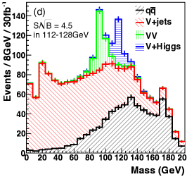
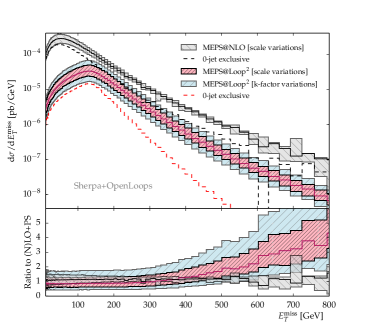
A third advantage of the production process is the perturbative control of the rate predictions. At Run II theoretical uncertainties are becoming the leading uncertainties in many Higgs measurements, especially when analyses utilize specific parts of phase space. In the right panel of Fig. 32 we illustrate the example of invisible Higgs searches, which experimentally relies on Higgs production at large . Above the threshold the one-loop diagram shown to the right in Fig. 31 becomes relevant, as we will discuss later. In the right panel of Fig. 32 we show the rates from the Drell-Yan or quark-initiated process and from the gluon fusion one-loop process. From the upper panel on the right, we see that even in this extreme phase space region with all partonic configurations are fully under control in perturbative QCD.
Finally, the -associated channel makes it especially easy to fully reconstruct the final state of the hard process. For example, we could search for alternative Lorentz structures of the interaction by looking at the reconstructed invariant mass . This is an advantage over the gluon fusion process discussed in Sec. 1, where the hard process includes the Higgs and possible hard jets, and the weak boson fusion process discussed in Sec. 2 with its experimentally challenging tagging jets.
One caveat is that not all four advantages listed above for the channel immediately apply to production. Missing transverse momentum is a major experimental challenge, and the experimental resolution on a transverse mass is always low. Nevertheless, the channel still allows for easy triggering through the hard lepton, the perturbative expansion is under control, and the hard process can be reconstructed reasonably well. The only problem is new backgrounds, for example single top and top pair production.
3.2 Precision predictions
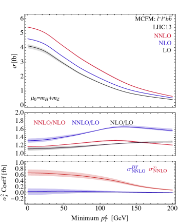
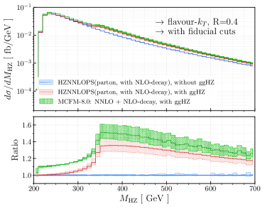
Given the Higgs signatures we target with its help, the process is a challenge for precision predictions. It is not sufficient to predict a total cross section, because the Caola et al. (2018), the invisible Higgs, and the effective theory analyses all rely on boosted phase space configurations, which make up only a small fraction of the total cross section. Nevertheless, we start by quoting the NNLO cross sections for the processes at a 14 TeV LHC, including the branching ratios of the and bosons to one lepton generation are Campbell et al. (2016)
| (B.18) |
A structural complication of the perturbative calculations arises from terms which do not scale with the leading-order Drell-Yan process. Normally, one would expect the higher-order production rates to scale like
| (B.19) |
However, for example the process shown in Fig. 31 proceeds through a heavy quark loop to which the heavy bosons couple. Similarly, the process includes Feynman diagrams where the Higgs couples to a closed top loop rather than the gauge boson. If we square these diagrams we find the scaling
| (B.20) |
including the top Yukawa coupling and a factor from the loop in the amplitude. The suppression of the new topology relative to the Drell-Yan process is small, namely , usually combined with the NNLO corrections because of the number of loops and the powers of , and only partly compensated by the larger parton densities for the gluon. However, while their contribution to the total cross section remains at the level, the relative importance of the different contributions changes for kinematic distributions.
In the left panel of Fig. 33 we show the rate above a minimum cut in computed to LO, NLO, and NNLO, including the top-loop contributions Campbell et al. (2016). In the upper two panels we see that the NNLO corrections are larger than the NLO corrections, which is an effect of the top-loop contributions and unique to the process. In the lower panel we see how the subprocess completely dominates the NNLO contribution. The drop towards larger minimum values is related to the softer gluon distributions in the proton. In the right panel we show a similar effect, now including the parton shower combined with a NNLO re-weighting method Astill et al. (2018). Clearly, the top-loop effects dramatically increase at the threshold , where the closed top loop develops an un-suppressed absorptive part. The slight difference between the two predictions including the top loop can be explained by a set of detector acceptance (fiducial) cuts on the leptons and the tagged -jets.
3.3 LHC Analyses
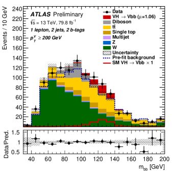
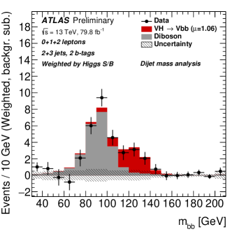
Using LHC data at 13 TeV, the focus of ATLAS and CMS in using the channel has been on Higgs decays to bottoms. ATLAS reports the two separate and one combined rate measurements from the 0-lepton, 1-lepton, and 2-lepton searches Aaboud et al. (2017),
| (B.21) |
Unfortunately, CMS does not report any actual cross section measurements, neither does ATLAS in their observation at collaboration (2018b). The combined rate measurement can be expressed as a single signal strength measurement of production combined with a Higgs decay to bottom quarks. ATLAS and CMS find collaboration (2018b); Sirunyan et al. (2018d),
| (B.22) |
The size of the error bars corresponds to the fact that none of these measurements has the significance required for a discovery of this signal. A simple check comes from searching for the corresponding di-boson signature from production combined with the decay collaboration (2018b); Sirunyan et al. (2018d),
| (B.23) |
In Fig. 34 we show two kinematic distributions for the 1-lepton channel, to illustrate the kinematic patterns of the different backgrounds. In the left panel we see that it is indeed possible to clearly separate the Higgs peak and the -peak. The larger Higgs mass helps with the signal extraction, because all backgrounds are rapidly dropping functions of . Because of the required two -tags and at most one additional jet, the +jets background with an actual heavy-flavor jet dominates in the low- range. Under the Higgs peak the top pair and single top backgrounds become equally important. The global agreement between the combined backgrounds in the side bands and the data is related to the post-fit nature of this plot. In this approach the individual background contributions are floated individually, and a scaling factor is then applied under the Higgs pole. In the right panel we show the Higgs signal after subtracting all backgrounds except the di-boson contribution, again highlighting the importance of the region.
Unlike the above analyses targeted at the decay of the Higgs boson to bottom quarks, we can also use the same final state to search for new physics in this channel Aaboud et al. (2018a). In the right panel of Fig. 34 we show the results for one of the signal categories, which is especially interesting: for a heavy resonance we expect that the two -jets coming from the Higgs decay can be boosted enough to become one observable jet. The invariant mass in the 1-lepton category is then computed by requiring that the lepton and the missing energy combine to an on-shell -boson. As a side effect of this analysis we see that there is no hint of any unexpected behavior of the channel all the way to TeV.
Additional searches using the production channel search for invisible Higgs decays. The corresponding CMS analysis Khachatryan et al. (2017) combines this channel with the WBF and the gluon fusion production mechanism. Because the WBF analysis was expected to be driving this search, we will discuss it in Sec. 2.
4 Associated and production
(100,60) \fmfsetarrow_len2mm \fmflefti1,i2 \fmfrightt1,h1,t2 \fmfgluon,width=0.6,lab.side=right,tension=2i1,v1 \fmfgluon,width=0.6,lab.side=right,tension=2v2,i2 \fmffermion,width=0.6,lab.side=left,tension=1t1,v1,vh,v2,t2 \fmfdashes,width=0.6,lab.side=left,tension=1vh,h1 \fmflabeli1 \fmflabeli2 \fmflabelt1 \fmflabelt2 \fmflabelh1 {fmfgraph*}(100,60) \fmfsetarrow_len2mm \fmflefti1,i2 \fmfrightt1,h1,t2 \fmffermion,width=0.6,lab.side=right,tension=2i1,v1,i2 \fmfgluon,width=0.6,lab.side=right,tension=1.5v1,v2 \fmffermion,width=0.6,lab.side=left,tension=1t1,v2,vh,t2 \fmfdashes,width=0.6,lab.side=left,tension=1vh,h1 \fmflabeli1 \fmflabeli2 \fmflabelt1 \fmflabelt2 \fmflabelh1 {fmfgraph*}(100,60) \fmfsetarrow_len2mm \fmflefti1,i2 \fmfrightt1,h1,t2 \fmffermion,width=0.6,lab.side=right,tension=2i1,v1,t1 \fmfphoton,width=0.6,lab.side=right,label=,label.dist=3,tension=1.5v1,vh \fmfphoton,width=0.6,lab.side=right,label=,label.dist=3,tension=1.5vh,v2 \fmffermion,width=0.6,lab.side=left,tension=1i2,v2,t2 \fmfdashes,width=0.6,lab.side=left,tension=1vh,h1 \fmflabeli1 \fmflabeli2 \fmflabelt1 \fmflabelt2 \fmflabelh1 {fmfgraph*}(100,60) \fmfsetarrow_len2mm \fmflefti1,i2 \fmfrightt1,h1,t2 \fmffermion,width=0.6,lab.side=right,tension=2i1,v1 \fmffermion,width=0.6,lab.side=right,label=,label.dist=3,tension=2v1,vh \fmffermion,width=0.6,lab.side=right,tension=2vh,t1 \fmfphoton,width=0.6,lab.side=right,label=,label.dist=3,tension=1.5v1,v2 \fmffermion,width=0.6,lab.side=left,tension=1i2,v2,t2 \fmfdashes,width=0.6,lab.side=left,tension=1vh,h1 \fmflabeli1 \fmflabeli2 \fmflabelt1 \fmflabelt2 \fmflabelh1
Top pair associated Higgs production
| (B.24) |
is the dominant channel with direct sensitivity to the top-Yukawa coupling, which from the fundamental physics perspective of Sec. 4 is one of the two most important parameters in the Higgs sector (the Higgs self-coupling being the other). In addition, it is crucial in allowing us to use the effective Higgs-gluon coupling to search for new particles contributing to the loop. We show two typical Feynman diagrams in Fig. 35. Consequently, production is central to the LHC Higgs phenomenology program. The measurement program includes all top decay channels as well as dominant and phenomenologically clean Higgs final states.
The production of a Higgs boson in association with a single top quark Diaz-Cruz and Sampayo (1992); Maltoni et al. (2001),
| (B.25) |
features an interference between Higgs emission off a -leg and Higgs emission of a top-leg, shown in Fig. 35. This allows us to constrain the sign of the top Yukawa coupling.
4.1 Motivation and signature
Early sensitivity estimates Airapetian et al. (1999) motivated top pair-associated Higgs production as the main discovery channel for a light SM Higgs boson. A more thorough subsequent analysis Cammin and Schumacher (2003) significantly decreased this estimate, and isolating production remains one of the experimentally most challenging tasks of the LHC Higgs program. Relevant channels are
| (B.26) |
where the latter two are similar enough on the detector level to be combined. Typically, analyses focus on fully-leptonic or semi-hadronic top decays, while fully-hadronic production is extremely challenging due to triggering and multi-jet backgrounds.
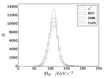
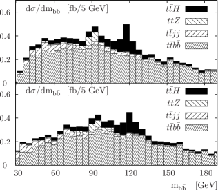
While it gives the largest signal rate, the Higgs decay suffers from a challenging signal vs background ratio of 15%. An improved discrimination of signal and background can be achieved by combining signal and background matrix elements into a likelihood to achieve a highly-adapted background rejection performance. For instance, the matrix-element method described in Sec. 3.2 should improve the situation Artoisenet et al. (2013b) and was adopted by CMS and ATLAS Khachatryan et al. (2015b); Aad et al. (2015e). Given the moderate signal vs. background ratio and the fundamental interest in the top Yukawa coupling, production serves as the show-case for some of the most advanced analyses approaches that are pursued at the LHC. With increasing luminosity we expect the combination with decays to dominate the analysis and provide the most robust and usable results.
The main challenge for observing in the channel is the combinatorics of the four -jets. Without a clear identification of the correct combination out of combinations and hence without information on the Higgs mass it is extremely difficult to define and control a background rejection Cammin and Schumacher (2003). One way to address this problem is deep learning. Comparing the performance of a method, a BDT, and a neural network based on the same observables, the deep neural network clearly gives the best results Erdmann et al. (2017). In the left panel of Fig. 36, we show the reconstructed Higgs mass from the three methods, compared to Monte Carlo truth. Motivated by the success of substructure methods in production Butterworth et al. (2008), it makes sense to also probe in a phase space region where the -jet combinatorics is automatically resolved by the boost of the decaying particles Plehn et al. (2010); Chatrchyan et al. (2016). The boosted analysis using subjet methods allows for the usual side-band analysis in to control the backgrounds, as shown in the right panel of Fig. 36.
Single top-associated Higgs production
| (B.27) |
has the potential to constrain the sign of the top Yukawa coupling relative to the coupling. These couplings have different signs in the Standard Model and current LHC measurements cannot yet fully distinguish between swapped Yukawa coupling signs Corbett et al. (2015a); Aad et al. (2016a) in the combination of the major production and decay channels, see below.
As a consequence of the destructive interference in the Standard Model, the top associated Higgs production cross section increases by a factor of about 15 when the top quark Yukawa interaction sign is swapped compared to the Standard Model, as shown in Fig. 39. Note that this would fall outside the assumptions of perturbative deformations of the Standard Model using dimension-6 SMEFT. While this effect is similar to the the partial decay width , which is small due to a cancellation between the virtual top and contributions the sign-degeneracy cannot be fully resolved using Higgs decay observables like alone Farina et al. (2013). Including single top-associated Higgs production, however, breaks the residual degeneracies as discussed in Farina et al. (2013); Biswas et al. (2013). This makes production an important part of the Higgs phenomenology program at the LHC.
Finally, single-top-associated Higgs production is particularly relevant in the search for for charged Higgs bosons in the decay Roy (1992); Assamagan and Coadou (2002). Charged Higgs boson from Higgs triplets can be searched for in gauge-induced pair production or in WBF, while charged Higgs bosons in a 2HDM or in the MSSM can only be produced through their fermion couplings, specifically a -increased bottom Yukawa coupling. The interaction then gives rise to a top-charged Higgs final state,
| (B.28) |
The main challenge in describing and extracting this signal is the treatment of the forward bottom jet Plehn (2003); Weydert et al. (2010), where a large invariant mass of the system induces a reasonably large logarithm, which in turn can be resummed through the use of bottom parton densities.
4.2 Precision predictions
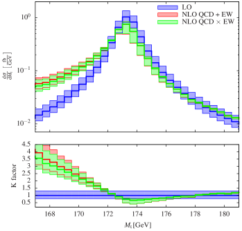
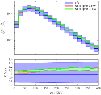
NLO QCD corrections moderately increase production by Reina and Dawson (2001); Reina et al. (2002); Dawson et al. (2003a, b); Beenakker et al. (2001, 2003). The cross section at in the Standard Model is Dittmaier et al. (2011)
| (B.29) |
However, given the complex analysis techniques, a precision prediction of the total rate falls short of the experimental requirements. Instead, we need a precise prediction of all kinematic distributions for the signal as well as for the irreducible background Bredenstein et al. (2010); Denner et al. (2012b); Gütschow et al. (2018). This includes the boosted regime, where we expect any analysis to collect most of its significance Plehn et al. (2014). Corresponding results are available to NLO in QCD Denner et al. (2012b) and including electroweak corrections Denner et al. (2017). In Fig. 37 we show the NLO effects on two key distributions for the signal. The dramatically increased tail in the reconstructed Higgs mass arises from non-recombined gluons and photons. While the NLO contributions are large and positive in the boosted Higgs regime, they lead to a relative drop in the boosted top regime.
First LHC cross sections for single top-associated Higgs production were provided in Ref. Maltoni et al. (2001); cross sections in the 5 flavor scheme are currently known to NNLO precision Brucherseifer et al. (2014) and NLO precision in the 4 flavor scheme Campbell et al. (2009); Demartin et al. (2015). The flavor scheme-averaged NLO prediction at in the Standard Model is Demartin et al. (2015)
| (B.30) |
This amounts to a moderate K factor of ). The dominant uncertainty of about 10% is related to the flavor scheme and scale dependencies.
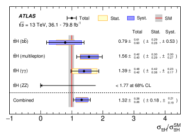
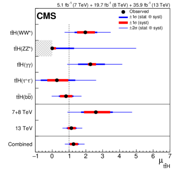
4.3 LHC Analyses
CMS has observed evidence for production in leptonic (including tau) final states Sirunyan et al. (2018f) at the level Sirunyan et al. (2018f); upon combining with run 1 data CMS reported a discovery at the level Sirunyan et al. (2018e) with a best-fit signal strength of
| (B.31) |
A comprehensive search for in the context of the Standard Model at 13 TeV most recently by ATLAS Aaboud et al. (2018b) combines results from and , as well as and at a luminosity of 79.8/fb. Combining these final states in a dedicated boosted decision trees allowed ATLAS to obtain a best fit value of the signal
| (B.32) |
which is consistent with the SM prediction, but shows a slight preference for overproduction with a signal strength
| (B.33) |
The ATLAS measurement amounts an observed significance of 5.1 standard deviations, and hence ATLAS provided the observation of top quark pair associated Higgs production in the Standard Model with the largest overall data set that has been considered in a Higgs analysis so far.
A fully hadronic analysis of is notoriously challenging which is apparent in the rather loose 13 TeV constraint observed by CMS Sirunyan et al. (2018g), which reports a best-fit signal modified constraint of . ATLAS constrains at 8 TeV Aad et al. (2016b).
CMS has recently looked for single top-associated Higgs production at 13 TeV Chatrchyan et al. (2017a) in the and Higgs final states, while the analysis is only available at 8 TeV Khachatryan et al. (2016a). The cross section limit that CMS obtains under the assumption of a flipped Yukawa coupling compared to the Standard Model is
| (B.34) |
The best-fit signal strength assuming SM couplings is , which amounts to an observed significance of 2.7. As can be seen from Fig. 39, the LHC has begun to exclude wrong-sign Yukawa couplings (under the assumptions quoted in Fig. 39).
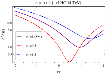
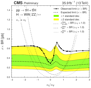
Additionally, charged Higgs production can be searched for in final states Aad et al. (2016c); Khachatryan et al. (2015c) or Aaboud et al. (2016b), as illustrated in Fig. 40.
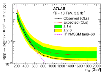
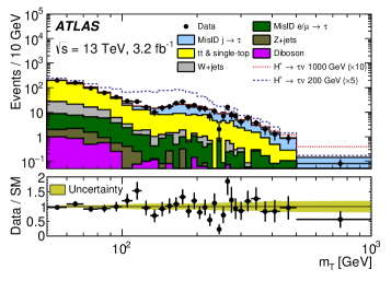
5 Exotic and rare decays
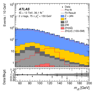
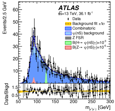
Constraining Higgs interactions through its decays to rare final states is a formidable experimental task, in particular because the expected signal count is tiny. Firstly, trigger criteria can be satisfied through, e.g. , observing the leptonic decay of the boson in associated Higgs production
| (B.35) |
This process, including the Higgs decay to charm branching ratio, has a cross section
| (B.36) |
Through adapted jet-tagging techniques the charm content of the Higgs candidate events can be tagged similar to -tagging, Fig. 41. These techniques are experimentally involved and are based on charmed meson decay phenomenology Aad et al. (2014a); Chatrchyan et al. (2014)).
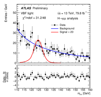
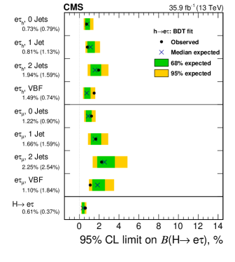
The second avenue as mentioned in Sec. 3.5 relates to Higgs decays with an easy to tag final state including photons, bosons and - and -flavored mesons (see also Aaboud et al. (2018f)). Summing over different Higgs production modes ATLAS has placed the limits Aaboud et al. (2018d)
| (B.37) |
These constraints are two to 5 orders of magnitude away from the SM expectations Bodwin et al. (2013); König and Neubert (2015). In the right panel of Fig. 41 we show how the different Higgs production modes contribute to the combined analysis. As expected for Run I, the gluon fusion process dominates the statistics-limited analysis.
Leptonic decays of the Higgs are Yukawa-suppressed in the Standard Model and the decay of the Higgs boson into to muons is highly suppressed at an expected branching ratio value of . The signature, however, is very clean as muons are easy to isolate and the mass resolution in the di-muon channel is high, Fig. 42. The inclusive search for the Higgs decay is dominated by gluon-fusion production, the main background is Drell-Yan production of two muons, and one of the major obstacles is that for the final state there are not many handles to separate signal and background aside from the invariant di-muon mass Han and McElrath (2002). The situation changes once the integrated luminosity allows us to combine rate Higgs decays with WBF production. In this case we can use the central jet activity to reduce the QCD background to the level of electroweak production, as discussed in Sec. 2. An appropriate multi-variate analysis of the WBF final state will then significantly enhance the reach of the LHC Plehn and Rainwater (2001); Cranmer and Plehn (2007). The current analysis based on inclusive Higgs production Aaboud et al. (2018e) constrains the signal strength in the di-muon decay channel to
| (B.38) |
which corresponds to an observed upper limit on at 95% confidence level. This improves the 7 and 8 TeV searches by factor of about two (see e.g. the individual CMS and ATLAS analyses of Refs. Khachatryan et al. (2015d); Aad et al. (2014b) as well as their combination Aad et al. (2016a)). The latest CMS 13 TeV analysis sets a CL constraint of Chatrchyan et al. (2017b).
Although lepton-flavor off-diagonal Higgs interactions are absent in the Standard Model, their observation at the LHC would be clear evidence of new physics beyond the Standard Model in the Higgs sector Diaz-Cruz and Toscano (2000); Han and Marfatia (2001); Harnik et al. (2013). This motivates searches for Han and Marfatia (2001) as performed by the CMS experiment Sirunyan et al. (2017c) and ATLAS Aad et al. (2015f), with current constraints in the (sub)percent range, Fig. 42 (right).
6 Global Higgs analyses
The ever increasing number of Higgs measurements, based on different production channels, decay channels, and phase space regions, calls for global analyses. As introduced in Sec. 7, the simplest approach starts from a Lagrangian with modified Higgs couplings to all Standard Model particles. This model can be incorporated in a consistent quantum field theory as an effective field theory including the Higgs scalar in the broken phase. An alternative effective theory approach includes the Higgs field as part of a doublet with the weak Goldstone modes. We will show results for this kind of analysis in Sec. 6.1. A general limitation of all effective field theory approaches is that they assume that all new particles are decoupled at the LHC. At the same time, the bases of higher-dimensional operators introduce a cutoff scale, above which we would have to resort to the full ultraviolet completion. An alternative set of hypotheses for global Higgs analyses are consistent ultraviolet completions of the Standard Model. It includes general extended Higgs sectors as well as their more predictive supersymmetric counterparts, as introduced in Sec. 5. We will quote some example results using these approaches in Sec. 6.2.
6.1 Effective theory
Because of the intermediate Higgs mass of GeV, there exists a multitude of Higgs signatures at the LHC. Global Higgs analyses are based on a set of Higgs production channels
-
•
gluon fusion, loop-induced by heavy quarks in the Standard Model (Sec. 1)
-
•
weak boson fusion, combining dominant -fusion and sub-leading -fusion (Sec. 2)
-
•
associated and production (Sec. 3)
-
•
associated and production (Sec. 4)
Ideally, each of these categories dominates an experimental signature. As discussed in Sec. 1.4, off-shell Higgs production and boosted Higgs production provide additional information mostly on the gluon fusion process. For precision Higgs analyses these production channels can be combined with SM-like decays
-
•
decays to fermions (Sec. 3.1)
-
•
tree-level decays to bosons (Sec. 3.2)
-
•
loop-induced decays (Sec. 3.4)
-
•
invisible Higgs decays , negligible in the Standard Model
These decays can be combined with each of the production processes, with the exception of gluon fusion Higgs production with a decay which is swamped by QCD backgrounds. Moreover, the rare decays and will only play a significant role for the upcoming LHC runs. A straightforward way of combining the corresponding LHC measurements are the coupling modifiers defined in Eq.(A.106) Zeppenfeld et al. (2000); Duhrssen et al. (2004); Lafaye et al. (2009). As discussed in Sec. 7.1. The notation is equivalent, provided we correctly separate the effective Higgs couplings to gluons and photons into modified couplings entering the SM loop diagrams and generic new loop contributions. On the quantum field theory side, the coupling modifiers can be interpreted as Wilson coefficients in an effective theory with non-linearly realized electroweak symmetry breaking Buchalla et al. (2017). Because the SM-like coupling modifiers have very little effect on kinematic distributions, at least at the Run I precision level, they can be extracted from measured total cross sections or so-called signal strengths
| (B.39) |
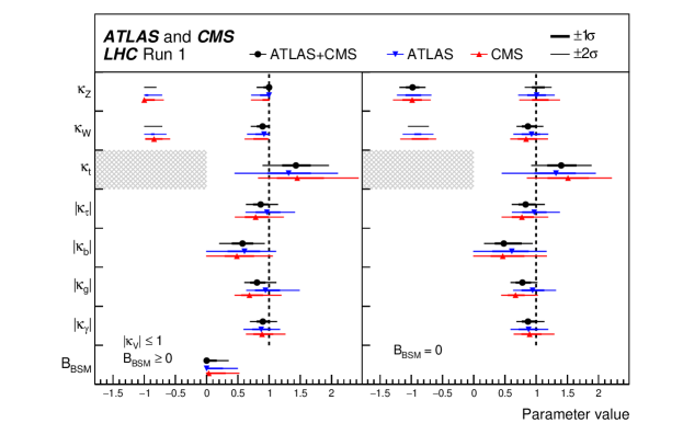
The main challenge of the global analysis is not to extract a decent central value for each coupling modifier based on a set of measured signal strengths. Given that we have not observed a significant deviation from the SM predictions, the question is how close the Higgs couplings are to their SM predictions. In other words, we need to carefully account for statistical, systematic, and theoretical uncertainties with full correlations between the observables and the predictions. ATLAS, CMS, and most theoretical collaborations rely on a likelihood approach with profile likelihoods for all nuisance parameters and irrelevant directions in model space.
In Fig. 43 we show the combined ATLAS and CMS limits on coupling modifiers or Wilson coefficients after Run I. Each limit is profiled over all other coupling modifiers, corresponding to the basic assumption that we do not expect new physics effects to only contribute to one Wilson coefficient. The two sets of limits shown in the figure are based on different assumptions about the total Higgs width, which enters every signal strength. We always start with the sum of the observed partial width as the lower limit to the total Higgs width. For the left set of measurements ATLAS and CMS assume that the Higgs couplings to the weak bosons are at most as large as in the Standard Model. This can be motivated by unitarity arguments Duhrssen et al. (2004) and allows us to include additional unobserved decays in the total Higgs width. For the right set of measurements the sum of the observed partial width, including all coupling modifiers, is identified with the total Higgs width. Finally, we can switch signs of all Higgs couplings, except for one global phase in the definition of the Higgs field. ATLAS and CMS fix the top Yukawa coupling to be positive, as indicated by the hatched areas. Sensitivity to the relative sign of Higgs couplings arises through the Higgs decay to photons, where the -loop and top loop interfere destructively. Looking at actual ultraviolet completions of the Standard Model, it is not at all obvious how one would switch the signs of and without having observed spectacular signs of new physics at the LHC. With extended Higgs sectors discussed in Sec. 5 it might be possible to switch the sign of a Yukawa coupling, most easily the bottom Yukawa, but again these kinds of interpretations should be taken with care. The safe assumption also based on our estimates of systematic and theoretical uncertainties would be
| (B.40) |
for all Higgs couplings analyses.
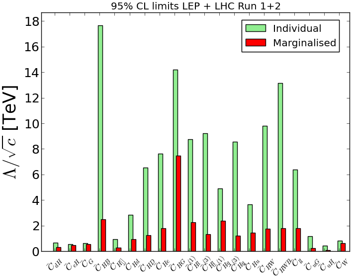
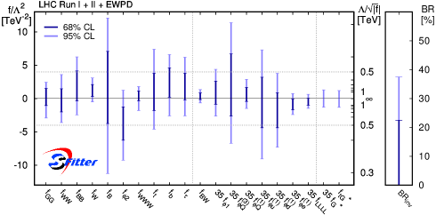
As described in Sec. 7.2, there are three shortcomings in the coupling modifier approach: experimentally, it does not (significantly) affect kinematic distributions and therefore excludes a wealth of experimental information from a global fit. Second, it is hard to reconcile with electroweak renormalizability, which means that we cannot match a percent level experimental precision with theory predictions. Finally, it does not allow us to combine information with electroweak measurements, be it electroweak precision data or di-boson production at the LHC. All three shortcomings can be cured by extending the model parameters to Wilson coefficients of an effective theory with linearly realized symmetry breaking in terms of the Higgs–Goldstone doublet. Technically, the global analysis is a straightforward extension of the previous analysis in terms of the coupling modifiers. It can be run on the same Higgs data set, which means that we can directly compare the results of the two approaches Corbett et al. (2015a). The main difference is that the gauge-invariant dimension-6 Lagrangian does not allow for separate modifications and .
| channel | distribution | #bins | max [GeV] | ||
|---|---|---|---|---|---|
| 8 TeV | leading | 350 | Aad et al. (2016d) | ||
| 575 | Khachatryan et al. (2016b) | ||||
| 450 | Aad et al. (2016e) | ||||
| 350 | Collaboration (2013) | ||||
| 13 TeV | 675 | collaboration (2018c) | |||
| 990 | Aaboud et al. (2018a) | ||||
| 1210 | Aaboud et al. (2018a) |
Because the effective theory leads to sizeable modifications of kinematic distributions through operators scaling like with the momentum flowing through a vertex, rather than . This makes it mandatory to include for instance transverse momentum distributions in weak boson fusion or associated production or the invariant mass in associated production. Technically, this complicates the analysis because we need to take into account bin-to-bin correlations in all uncertainties. On the other hand, from the scaling of the effective operators we also know that most of the relevant information will come from the highest reliable bins in these kinds of distributions. The corresponding momentum typically scales with the momentum flow through the effective vertex and determines the reason in the new physics scale . In Fig. 44 we show results from two global EFT analyses including Higgs and di-boson measurements at the LHC. While it is useful to express the limits in terms of , i.e. the prefactor of the effective operator in the Lagrangian, the relevant physics is typically encoded in the re-scaled new physics scale . The main change compared to the Run I legacy results is the quality of the different fermionic decay measurements, including , strongly correlated with the effective Higgs-gluon coupling included as . The long list of channels is nicely illustrated in Fig. 38. The appearance of reflects the fact that the fit combines Higgs measurements with di-boson production channels at the LHC. This additional information is crucial to remove strong non-Gaussian features and correlations from the pure Higgs analysis. Comparing the LHC limits from di-boson production on anomalous triple gauge couplings to LEP limits on the same parameters we see that the LHC has surpassed the LEP precision due to its larger momentum flow through the corresponding triple gauge vertices. This effect is not linked to the linear EFT description and also appears in the not gauge-invariant parametrization of Eq.(A.123).
Given the accuracy achieved at the LHC Run II it turns out that we cannot simply ignore operators which violate custodial symmetry at tree-level. Instead, we need to include those operators and fermionic operators leading to anomalous gauge couplings Baglio et al. (2017); Alves et al. (2018); Franceschini et al. (2018) and combine the LHC fit with electroweak precision data Ellis et al. (2018); da Silva Almeida et al. (2018); Biekötter et al. (2018). A similar approach is advertized in the Bayesian analysis of Ref. de Blas et al. (2016). Focussing on the marginalized, profile likelihood result, the operator looks much more constrained. This is related to the fact that the corresponding SM structure only appears at loop level and that unlike in Eq.(A.114) the loop factor is not included in this definition of the Wilson coefficient. The operators affecting the fermion couplings of the weak bosons appear in the LHC signals, but they are largely constrained by electroweak precision data. The fact that the limits on these Wilson coefficients are similar to the LHC limits confirms the observation that in the Higgs sector the LHC really has been turned into a precision experiment.
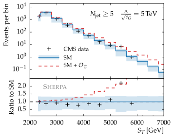
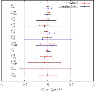
The appearance of the operator in the Higgs fit shown in Fig. 44 points towards the need to include information from entirely different LHC searches. The main reason is that an anomalous triple gluon interaction
| (B.41) |
will affect every LHC process. This not only includes Higgs production Ghosh and Wiebusch (2015); Dawson et al. (2015), but also top pair production Simmons (1990); Cho and Simmons (1995); Buckley et al. (2016, 2015) and jet production Dixon and Shadmi (1994); Krauss et al. (2017). Given the interference structure with the Standard Model and the available kinematic regimes, it turns out that this coupling is best probed in multi-jet production at the LHC. For example the kinematic variable
| (B.42) |
combined with high jet multiplicities, usually used to search for black holes at the LHC, can be used to probe the anomalous triple gluon coupling to very large scales Krauss et al. (2017),
| (B.43) |
In Fig. 45 we show the leading distribution entering this analysis. The reach of the LHC is, as usual, linked to the maximum momentum flow through the relevant vertex in the hard process.
Finally, the strong link between the Higgs and top sectors call for a combined analyses of the respective dimension-6 Lagrangians. Global top sector analyses are already available Bernardo et al. (2014); Buckley et al. (2016, 2015); Barducci et al. (2018) and lead to similar limits on the new physics scale as global Higgs analyses. As an example we show the results of an EFT fit to abundant top physics results at the LHC in the right panel of Fig. 45. While intermediate Higgs bosons are phenomenologically not relevant for inclusive top final states, dimension 6 operators like and the chromo-magnetic moment of the top quark represented by
| (B.44) |
impact inclusive top physics, the latter upon sending the Higgs to its vacuum expectation value. This also highlights the spirit of EFT measurements that predict dedicated correlations between different final states on the basis of gauge symmetry and particle content. The individual constraints from the top fit, Fig. 45, show that the limit on from top physics is weaker than the one obtained from multi-jet production, but the constraint on amounts to a scale . This will improve with higher luminosity Englert et al. (2016b), with perturbative uncertainties expected to be the limiting factors. As expected, this scale approximately corresponds to the largest energy scale probed in the analysis included in Ref. Buckley et al. (2016).
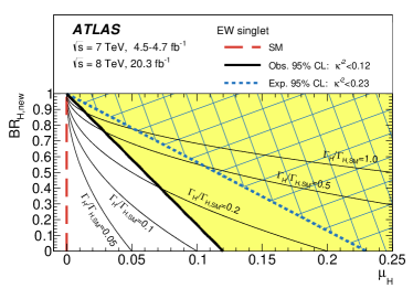
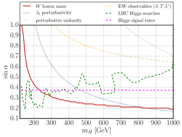
The latter point picks up on a common problem with all effective theory analyses related the self-consistency of the approach. It always requires that all new particles can be safely integrated out and do not contribute as propagating degrees of freedom to a given observable. At the LHC this can be a problem, first because of the large available partonic energy for rare events with a parton momentum fraction , and second because of the very slow decoupling of -channel processes. On the phenomenological level, an easy and straightforward way to test the validity of the effective theory is the appearance of mass peaks. In other words, we can analyze enhanced tails for example of transverse momentum distribution, but only to a point where we see a peak. This requirement is hard to quantify. On the other hand, we can just consider EFT analyses ways to systematically search for anomalies in some phase space region of some processes, which we will then try to explain in terms of a much wider range of models. This approach largely gets rid of the consistence criterion and instead leaves us with experimental results on the dimension-6 Lagrangian which some might find hard to interpret in terms of actual models. Similarly, theoretical uncertainties derived for example from the truncation of the dimension-6 Lagrangian do not have to enter the experimental analysis and can instead be considered as part of the interpretation of the results in terms of more interesting, full models. This link can be systematically explored in terms of a proper matching procedure in the presence of electroweak symmetry breaking Freitas et al. (2016).
6.2 Ultraviolet completions
For concrete models, correlations between different channels can be exploited as functions of the new physics parameters to set tight constraints on the presence of new states. The experiments typically perform such analyses for well-motivated extensions of the Standard Model such as two Higgs doublet models or supersymmetric scenarios.
The Higgs singlet model is severely restricted by limits on the Higgs couplings to SM particles, by direct searches for the second Higgs particle, , and by precision electroweak measurements. In this section, we assume . If (i.e. it cannot decay to ), then the branching ratios are identical to those of the Standard Model and the production rates are uniformly suppressed by , leading to a limit from a global fit of Aad et al. (2015b). Once the decay is allowed, the total Higgs width and the branching ratios can be significantly altered. It is possible to get branching ratios of for . The limits from ATLAS are shown in Fig. 46. Direct limits on the mass of the heavier Higgs boson can be extracted by re-purposing the SM heavy Higgs search limits and are shown in Fig. 46. The strongest limits for a heavy come from the boson mass López-Val and Robens (2014), while direct searches coupling measurement limits are similar.
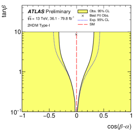
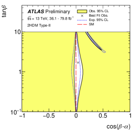
The 2HDM can be studied both by analyzing Higgs couplings and by direct searches for the heavy and . Coupling fits from Run-2 in the Type-I and Type-II models are shown in Fig. 47 and demonstrate that the couplings are highly restricted. Type-I models require from the coupling fit, with even tighter bounds for . Since the associated production of is suppressed by , these modes are much smaller in the 2HDM than for a SM Higgs boson of the same mass. Gluon fusion and production rates are (in the alignment limit), and so are promising channels. In Type-II 2HDMs, the limits from the coupling fit is quite stringent and requires and so the model must be quite close to the alignment limit. The associated productions modes in Type-II 2HDMs are highly suppressed relative to the Standard Model, while the gluon fusion mode remains large Craig et al. (2015). The heavier Higgs bosons can be searched for directly, with the most promising channel being .
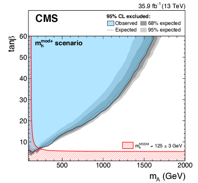
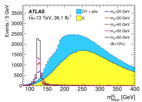
Production rates for the MSSM Higgs bosons are often compared for small and large for the specific benchmark point
| (B.45) | ||||
that is part of the more comprehensive benchmarking program carried out after the Higgs boson discovery Carena et al. (2013). For small , gluon fusion is always the dominant production channel for and for with . In the small region, the channel dominates. For large , the and channels always dominate, due to the enhanced couplings to quarks. At large , the most stringent limits come from shown in Fig. 48.
Another possibility that arises in supersymmetric scenarios is the exotic decay of the Higgs boson into two pseudo-scalar bosons, followed by subsequent decays into quarks, photons and leptons. ATLAS and CMS have studied a plethora of channels at 13 TeV already (see Fig. 48 right for an example). Searches exist in the Aaboud et al. (2018g), Aaboud et al. (2018h), Aaboud et al. (2018i), Sirunyan et al. (2018i); Aad et al. (2015g), and Sirunyan et al. (2018j) final states. So far, no evidence for such decays has been observed and branching fraction constraints in percent range (assuming SM production of the Higgs boson) have been obtained in the region depending on the model-dependent decay phenomenology and mass of the pseudoscalar .
C Perspectives
Future experiments to further Higgs physics beyond the capabilities of the LHC divide broadly into two concepts. First, Lepton colliders that provide a precision investigation of Higgs phenomenology at the weak scale. The strategy that motivates such machines stand in the long tradition of a precision spectroscopy that ensues after a discovery, much like the LEP boson precision program that followed the Super Proton Synchrotron (SpS) which facilitated the discovery of and bosons. Crucial to the extraction of a plethora of Higgs couplings is a range of accessible lepton collider energies (see below).
However, the Standard Model being complete as a renormalizable quantum field theory after the Higgs discovery, a precise understanding of the weak Higgs boson couplings might not necessarily point in the direction of a more fundamental theory beyond the weak scale. This situation is qualitatively different to the early boson precision days, when the Higgs boson and the top quark were the missing pieces to obtain a theoretically well-defined theory. In this sense, any precision results informed Higgs physics directly. After the Higgs discovery, only tensions of the Standard Model can be revealed, but no clear connection to UV physics can be drawn unless new physics is directly discovered.
This insight motivates a second avenue of future colliders, namely another (possibly ultimately final) push for a hadron-hadron collider extrapolated from existing LHC technology. With center of mass energies hypothesized to push up to 100 TeV, such a machine can not only access Higgs couplings that are difficult to constrain at the LHC or lepton colliders, but also opens up the a new range of energy to observed particle thresholds and resonances, thereby breaking the status quo of the Standard Model as a complete renormalizable theory.

1 Future lepton colliders
A clear and technologically well-developed avenue for Higgs physics is coupling measurements at proposed colliders through the abundant production of Higgs bosons in a clean environment. There are two classes of proposals for such Higgs factories: linear and circular machines. A well-studied linear collider concept is the International Linear Collider (ILC) planned with a center-of-mass energy between 250 GeV and 500 GeV, in principle upgradable up to 1 TeV. The technical design report has been published in 2013 Behnke et al. (2013); Baer et al. (2013); Adolphsen et al. (2013a, b); Abramowicz et al. (2013), and can therefore be considered as the most mature proposal of a future collider.
The Higgs program of such a machine Fujii et al. (2017, 2015); Arbey et al. (2015) is based on precision determinations of Higgs couplings. The level of uncertainties at an collider are are very different from the LHC Klute et al. (2013); Fujii et al. (2017); Han and Liu (2013): QCD is less of a nuisance than at hadron colliders, and electroweak corrections are typically a factor 10 to 100 smaller than QCD corrections. Initial state QED radiation and Beam-strahlung are well understood Boogert and Miller (2002), leading to the possibility of very precise measurements as well as very precise theoretical interpretations. The ILC can run on the peak of the Higgs–strahlung cross section as well as at larger center-of-mass energy Fujii et al. (2017). The latter option is particularly useful to extract precise information from -fusion Higgs production as well as to measure Higgs production associated with top-quark pairs. The linear design is also used in the Compact Linear Collider (CLIC) proposal; its conceptual design report was released in 2012 Aicheler et al. (2012) and the Higgs physics program of such a machine is discussed in Ref. Abramowicz et al. (2017). CLIC aims to achieve collisions at up to 3 TeV, thus enabling measurements of various Higgs processes at large momentum transfers which enables a fine grained picture of Higgs interactions in particular when considered in the framework of EFT modifications Ge et al. (2016); Durieux et al. (2017); Ellis et al. (2017); Barklow et al. (2018a).
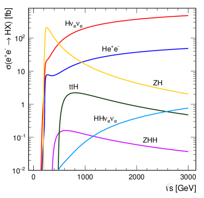
| collider | [GeV] | luminosity [] |
|---|---|---|
| HL-LHC | 14000 | 3 |
| FCCee/CEPC-base | 240 | 4 |
| FCCee/CEPC-350 | 240/350 | 4/1 |
| ILC-stage | 250 | 2 |
| ILC-base | 250/350/500 | 0.5/0.2/0.5 |
| ILC-lumi | 250/350/500 | 2/0.2/4 |
The second design possibility is a circular collider (FCC-ee/TLEP Bicer et al. (2014) or CEPC Ahmad et al. (2015a, b)) that could produce very large numbers of events close to threshold. The strength of circular machines compared to linear baselines is the large luminosity that can be achieved at the price of lost control over the beam conditions due to bremsstrahlung. In particular, polarizations of the beams cannot be controlled, which is one of the strengths of the linear collider setups to measure complementary coupling aspects of Higgs physics Fujii et al. (2018). For instance, while in the Higgs–strahlung process left-chiral and right-chiral fermions couple to the –boson with different coupling strengths, only left-chiral fermions induce -fusion Higgs production. The proposed integrated luminosity and energies for future colliders are given in Tab. 10 (based on Ref. Dawson et al. (2013a)), but are therefore not directly comparable.
Both circular and linear concepts feature runs at lower energies to precisely determine the electroweak input parameters before measurements at higher energies can be made with high precision. This includes collecting data at the and pair thresholds similar to LEP before precision measurements at the and top thresholds are performed. While a pair program could be motivated from a -violation perspective through constraining anomalous couplings, the expected small effects Corbett et al. (2017) mean that pair production is mainly used for data-driven analyses.
At an collider the two main Higgs production mechanisms are Higgs–strahlung and -fusion Higgs production Jones and Petcov (1979) as shown in Fig. 49. The energy dependence of these processes is given in Fig. 50. The -channel fusion process grows with energy and dominates for energies above , Higgs-strahlung and fusion can be complemented by the associated production of top quark pairs and a Higgs boson and by Higgs pair production in association with a -boson. Representative (leading order, unpolarized) cross sections at 350 (3000) GeV are Abramowicz et al. (2017)
| (C.1) | ||||
In the process , the observation of the boson can be used to tag the process (up to corrections from radiation) independent of the Higgs boson decay channel, and the branching ratios of the Higgs boson are observed directly. The Higgs mass can be measured precisely with an accuracy of Yan et al. (2016) through the recoil of events, Fig. 51. Similarly, the ILC can constrain an invisible Higgs branching ration as low as 0.4% Asner et al. (2013) (such constraints, however, are model-dependent, as already mentioned).
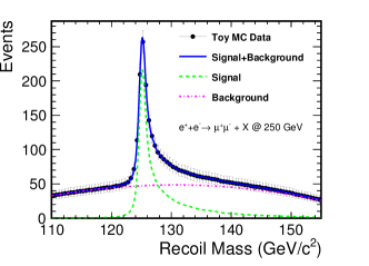
The Higgs coupling strengths are obtained by noting that
| (C.2) |
Assuming that the Higgs couplings are related to the SM couplings by the factors described previously, then
| (C.3) |
This yields a measurement of the total Higgs width with the same assumptions as for the LHC: that is, that there are no non-SM tensor structures for the interactions of the Higgs boson with the SM fermions. As the Higgs branching ratio into is small, this requires a significant amount of luminosity. Another way to determine the Higgs width is based on four measurements Aguilar-Saavedra et al. (2001); Baer et al. (2013) of both production processes shown in Fig. 49,
-
1.
Higgs–strahlung inclusive: ,
-
2.
Higgs–strahlung with a decay to : ,
-
3.
Higgs–strahlung with a decay to : ,
-
4.
-fusion with a decay to : ,
involving the four unknown parameters , , , and . Schematically, the total width can be extracted as
| (C.4) |
This is demonstrated in in Fig. 52, where we show the projected coupling measurements from Ref. Lafaye et al. (2017), assuming that the total width can be computed as the sum of all observed partial widths plus contributions from second-generation fermions. The comparison of FCCee and ILC projections assumes a combination with the expected HL-LHC results and it is apparent that the linear and circular designs will both be limited by the theoretical uncertainty in extracting Higgs couplings from observed event rates. The general pattern we see in Fig. 52 is that for all couplings with the exception of the FCCee base design, the ILC base design, and the ILC staging design give comparable results. As a representative value to be compared with sensitivities of potential future hadron machines, the fit of Lafaye et al. (2017) gives a best Yukawa coupling precision of
| (C.5) |
The GeV ILC will probe the -fusion process combined with all main decay modes, allowing for a higher overall precision.
Improving on studies based on Higgs coupling strength modifiers, the most generic Higgs coupling modifications from integrated-out UV states at both the LHC and colliders should be analyzed in terms of an effective field theory approach. The corresponding frameworks are discussed in Sec. 7. This introduces new interactions and thereby breaks the naive correlations between different production modes at different energies expressed in the kappa framework. This has profound consequences Ellis et al. (2017); Ellis and You (2016); Di Vita et al. (2018); Barklow et al. (2018b); Durieux et al. (2017); Barklow et al. (2018a) for the Higgs coupling extractions as can be seen from Fig. 53.
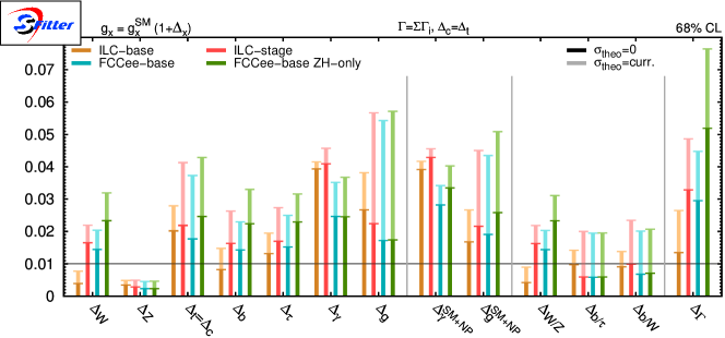
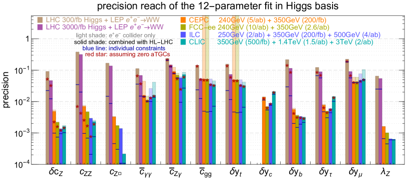
The presence of different Lorentz structures in the EFT framework induces momentum dependencies in the Higgs interactions Hagiwara et al. (1993b); Gonzalez-Garcia (1999). This means that there is a gain in information when pushing lepton colliders to larger energy due to the energy-dependent cross section enhancements. This is clearly shown for the direction , which is not directly related to Higgs physics but demonstrates clearly the impact of energy coverage. In addition, the polarization at the ILC can be used to obtain an increased number of observables (relative to an unpolarized collider), potentially yielding precisions on EFT couplings at the sub-percent level Barklow et al. (2018b).
One particular coupling that is expected to be only poorly constrained at the LHC even when considering large luminosities is the Higgs self coupling. Lepton colliders close this gap at least partially. Direct sensitivity to the Higgs self-interactions requires the production of (at least) a Higgs pair through weak boson fusion and and/or production, see Fig. 50. As can be seen there, energies well above the 240 GeV threshold are required. CLIC with its target energy of 3 TeV is particularly suited to achieve such a measurement via weak boson fusion with large statistics and projections predict a measurement of the trilinear Higgs coupling at the
| (C.6) |
at 1.4 (3) TeV collisions Abramowicz et al. (2017). Exploiting the threshold, similar analyses can be performed in this channel at the high energy ILC option, and constraints on the Higgs self interactions can be obtained in a global fit Di Vita et al. (2018); Barklow et al. (2018b).
2 Future hadron colliders
The precision spectroscopy of the Higgs sector that is possible at lepton colliders is to be compared with that obtained by pushing the LHC’s energy frontier further using proton-proton collisions at up to 100 TeV Contino et al. (2017); Golling et al. (2017); Mangano et al. (2017). While such a machine offers the opportunity of directly observing a more fundamental scale of physics, a precision Higgs program remains at the core of these proposals. This is linked to developments at the LHC, where we have learned how to control experimental systematics to the level of a few percent, how to provide theory predictions for hard processes to a similar level, how to precisely simulate events from first-principles QCD in a multi-jet environment, and how to use jets in many precision analyses. In the following we focus on a selected range of Higgs-relevant processes that demonstrate the improvement that can be achieved at such machines compared to the LHC, and how measurements in these channels will compare against lepton collider concepts.
2.1 Higgs pair production

The last parameter in the Higgs potential of the Standard Model, that is likely to be left only poorly constrained even after the HL-LHC, is the Higgs self-coupling. The direct measurement is based on gluon fusion-induced Higgs pair production Eboli et al. (1987); Dicus et al. (1988); Glover and van der Bij (1988), which receives contributions from a triangle loop diagram combined with the Higgs self-coupling and from a box diagram, as shown in Fig. 54. Over most of phase space, the box contribution completely dominates the total rate. However, there exist three phase space regions which provide information on the Higgs self-coupling Gonçalves et al. (2018); Buchalla et al. (2018), which corresponds to a modification in the effective field theory language (for enhanced derivative interactions see e.g. Goertz et al. (2015); Azatov et al. (2015b); Gillioz et al. (2012); Dawson et al. (2013b); He et al. (2016)). First, there is the threshold region Plehn et al. (1996); Djouadi et al. (1999); Baur et al. (2002); Li and Voloshin (2014)
| (C.7) |
The effective Higgs–gluon Lagrangian illustrates the threshold cancellation between the diagrams at the amplitude level,
| (C.8) |
where and in the Standard Model. While the heavy-top approximation is known to give a poor description of the signal kinematics as a whole, this cancellation at threshold remains as an approximate feature Borowka et al. (2016a). Any significant deviation from the SM value of the self-coupling will spoil this cancellation and lead to an increased rate at threshold, no matter if the self-coupling is smaller or larger than in the Standard Model. Second, an enhanced sensitivity to the self-coupling appears through the top threshold Glover and van der Bij (1988). The triangle contribution shows a distinctive kink at Georgi et al. (1978)
| (C.9) |
This is similar to the decay , as shown in Eq.(A.30) with replaced by . This is the leading effect when we search for an anomalous Higgs self-coupling. The same absorptive imaginary part also leads to a significant dip around GeV Dolan et al. (2012); Barr et al. (2015) if we parameterize the signal phase space this way. The destructive interference effect is shown in the left panel of Fig. 56, indicating that an increase in the self-coupling will be clearly visible as a dip relative to the SM distribution. Finally, the triangular and box amplitudes have a generally different scaling in the high-energy limitPlehn et al. (1996); Chen and Low (2014); Azatov et al. (2015b)
| (C.10) |
Here, the triangle with the intermediate Higgs propagator features an explicit suppression of either or , whereas the box diagrams drops more slowly. Whenever we can reconstruct the di-Higgs final state, an obvious way of extracting the Higgs self-coupling is through an shape analysis Bauer et al. (2017). We can use a maximum likelihood analysis Cranmer and Plehn (2007) to show that most of the significance for an anomalous self-coupling comes from around GeV Kling et al. (2017); Gonçalves et al. (2018).
In Fig. 55 we show the cross sections for different Higgs pair production channels as a function of the collider energy. As expected, gluon fusion is the dominant process. The rates for alternative production mechanisms are at least one order of magnitude smaller, with no obvious advantages of those channels at the analysis level. At the 13 TeV LHC the cross section is
| (C.11) |
computed at NNLO+NNLL de Florian and Mazzitelli (2013, 2015); de Florian et al. (2016b) including NLO top-mass effects Borowka et al. (2016a); Heinrich et al. (2017); Borowka et al. (2016b); Grazzini et al. (2018). LHC projections by CMS put the sensitivity in the range of at Chatrchyan et al. (2017c) at the LHC. The rare but clean channel Baur et al. (2004) will likely play the dominant role, although Baur et al. (2003); Dolan et al. (2012) can contribute significantly given recent level 1 trigger upgrades that have allowed CMS to reach hadronic di- tagging with a efficiency at an acceptable fake rate.
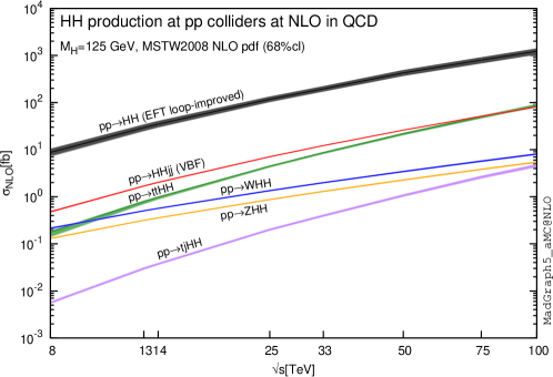
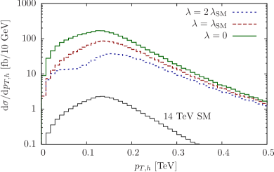
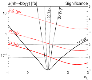
Going from 13 TeV proton-proton collisions to 27 TeV (HE-LHC) and on to 100 TeV (FCChh) increases the Higgs pair production rate significantly, as seen in Fig. 55. If we combine this with an expected luminosity of up to (HE-LHC) or (FCChh), the measurement of the Higgs self-coupling becomes a promising motivation and benchmark for further pushing the high energy frontier. In particular, the statistics-limited process at the LHC predicts 5k events already at the HE-LHC. Using a binned likelihood analysis for including detector effects and realistic efficiencies, we expect a reach Gonçalves et al. (2018)
| (C.12) |
with a very slight margin of error due to the expected detector effects and -tagging efficiencies Contino et al. (2017). Only the Higgs tri-linear coupling is varied in this analysis. We can compare this result to the expected reach using all available phase space information, shown in the right panel of Fig. 56. The key feature of these curves is that they do not feature an alternative minimum at very large anomalous self-couplings, predicting a SM-like total cross section from inverting the relative size of the triangular and continuum contributions.
If we go beyond a simple modification of the Higgs potential of the Standard Model the SMEFT framework introduced in Sec. 7.2 is the appropriate framework to study an anomalous Higgs self-coupling. Among the operators listed in Eq.(A.113) two modify the triple Higgs coupling, through an constant shift and through a momentum-dependent shift. On the other hand we know that also modifies all Higgs couplings through a wave function renormalization of the physical Higgs field, so we need to add to a global Higgs analysis and include Higgs pair observables, ideally covering all the distinct kinematic regimes discussed above. In Fig. 57 we show projections for a future 27 TeV collider, combining the global Higgs and gauge analyses extrapolated from Ref. Butter et al. (2016b), the invisible Higgs searches extrapolated from Ref. Biekötter et al. (2017), and the Higgs pair analysis of Ref. Gonçalves et al. (2018). We can then compare the expected limits on from a specific search for a modified Higgs self coupling with the expected limits from a global analysis, profiled over all other Higgs and gauge operators. For the former, we can translate the 15% measurement from Eq.(C.12) into TeV. While the effects of and can be separated through the different kinematic regimes, the global correlations nevertheless weaken the corresponding expectations to GeV, for an optimistic projection of systematic and theory uncertainties.
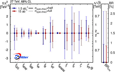
The kinematics for production links the two sensitive phase space regions to the suppressed threshold of the hard production process. Going from the LHC to a 100 TeV collider, the production rate of Higgs pairs with a hard jet grows by a factor around 80, significantly faster than the total production rate Ferreira de Lima et al. (2014); Gonçalves et al. (2018). This defines a novel phase space configuration with , where a collimated Higgs pair recoils against a hard jet. This jet might even be used to trigger the event. As a consequence, the phase space region is washed out across and . The reduced total rate of this process naturally points to larger Higgs decay rates such as . For this signature, subjet analyses allow us to to reduce the dominant backgrounds, especially when the decay dominates the recoil against the hard jet while the softer Higgs is reconstructed in final states. Relying on this configuration, a precision of
| (C.13) |
can be achieved at 68% C.L. Banerjee et al. (2018).
2.2 Associated production
Following Sec. 4 the second most interesting parameter in the Higgs sector is the top Yukawa coupling, leading to problems with vacuum stability in the Standard Model. As discussed in Sec. 4, the measurement of the top Yukawa coupling is best done in production. At the LHC, this channel is severely limited by experimental systematics and theory uncertainties. ATLAS and CMS expect a measurement of the top Yukawa coupling at the 10% level for the HL-LHC Aad et al. (2014c); Chatrchyan et al. (2017c). This limited precision leaves a large parameter space of UV models unconstrained. For example in composite Higgs scenarios it corresponds to a strong interaction scale around TeV, barely larger than the direct LHC reach.
Going to a 100 TeV collider, the production cross section increases dramatically to
| (C.14) |
as illustrated in Fig. 58. While the increased rate does not automatically help us control the systematic and theory uncertainties, it allows us to focus on phase space regions which are less prone to those limitations Mangano et al. (2016). As discussed in Sec. 4 one of those phase space regions is boosted production Plehn et al. (2010). It automatically solves the -jet combinatorics and allows for a side band analysis in . In addition, we can control uncertainties, for example from parton densities, by evaluating the ratio
| (C.15) |
over phase space Mangano et al. (2016). The reference process features the same top decays as the signal, while the hard process is entirely determined by the gauge structure of the Standard Model.
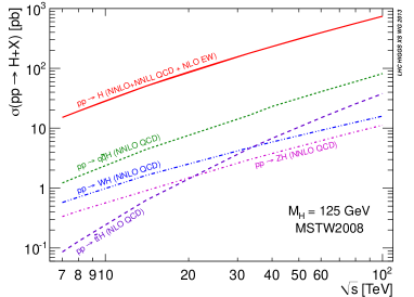
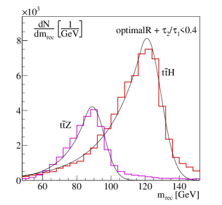
Note that we can expect to see the -peak in the distribution next to the Higgs peak Plehn et al. (2010), so the 100 TeV analysis will be based on the two-peak fit on top of the continuum background shown in the right panel of Fig. 58. In the signal region of the distribution, the boosted analysis leads to signal-to-background ratios around and a huge signal significance. It should allow us to measure the top Yukawa coupling with an uncertainty Mangano et al. (2016),
| (C.16) |
2.3 Invisible Higgs decays
A third benchmark channel for future hadron colliders are invisible Higgs decays. From the LHC we know that they can be best searched for in WBF Higgs production Biekötter et al. (2017), as discussed in Sec. 2. This electroweak process is much less prone to theory uncertainties than the usual QCD processes and should therefore allow us to systematically define precision measurements at a 100 TeV hadron collider Goncalves et al. (2017); Jager et al. (2017). In Fig. 59 we show the main kinematic features of the WBF process at a 100 TeV collider, compared to the LHC. First, we see that indeed the transverse momentum distributions of the tagging jets are defined by the -mass, with a peak around 70 GeV. For the 100 TeV collider we observe a slight change in the spectrum when we limit the tagging jet rapidities to , reflecting a preference for a slightly larger rapidity coverage at higher energies. In the right panel we show the number of jets in the different signal and background processes, which reflects the different Poisson and staircase scaling patterns Gerwick et al. (2012). This jet activity serves as the main handle in separating the WBF and gluon fusion contributions to production in a precision measurement.
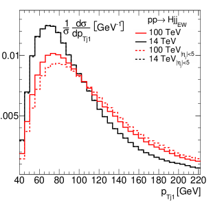
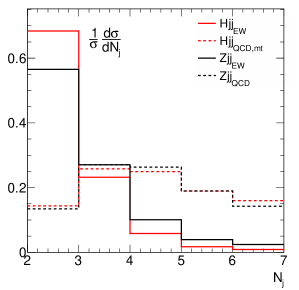
As for the Higgs pair analysis discussed in Sec. 2.1, a WBF analysis at a 27 TeV or 100 TeV collider benefits from including jet radiation in the signal process. We can for example define 2-jet and 3-jet signal and background samples by (i) vetoing a third jet for and (ii) requiring a third jet with and vetoing a fourth jet for Bernaciak et al. (2015); Goncalves et al. (2017). A typical jet veto scale is GeV. We can then use the , , and distributions to search for invisible Higgs decays and expect a reach of Goncalves et al. (2017)
| (C.17) |
In both cases the systematic uncertainties become the limiting factor. It might be possible to use the large statistics of mono-jet production to search for invisible Higgs decays in the process +jet Feng et al. (2006). However, there does not exist a reliable signal and background study, and the sizeable systematic and theory uncertainties in the underlying QCD process will limit the measurement of this branching ratio.
3 Theory for modern analyses
One of the key challenges of contemporary phenomenogy is to keep track with the experimental analysis strategies, which could allow us to turn the LHC into a precision experiment. In this section we will review the ideas behind some of the most relevant advanced analysis techniques and describe the corresponding challenges and novel ideas to theoretical LHC physics. We will show how these techniques are already applied at the LHC and how a coherent effort between experiment and theory will help us to make the best possible use of LHC data, in the Higgs sector and elsewhere.
Historically, LHC analyses have started with identifying phase space regions with a large signal-to-background ratio and extracting them by applying cuts on well-defined kinematic observables. A simple example is the mass window in in the Higgs discovery. A measurement is then based on counting events and comparing them to the background-only and the signal-plus-background predictions, using Poisson or Gaussian statistics. Assuming a discovery is quantified in terms of the statistical significance we typically apply a kinematic cut if it improves for a given luminosity. This kind of analysis has the fundamental disadvantage that there will always be kinematic observables and phase space regions which do not contribute to the analysis. Multi-variate analyses for example using boosted decision trees define cuts as non-trivial surfaces in the multi-dimensional phase space, but still remain cut-and-count analyses.
One way to improve these analyses is to change the way we organize events. Instead of a kinematic observable, we can define histograms in terms of any variable we want. The problem of finding the best test statistics for a given hypothesis test leads us to the Neyman-Pearson lemma, optimal observables introduced in Sec. 3.1, and the likelihood ratio discussed in Sec. 3.2. We can even classify events by some kind of boosted decision tree output variable without an obvious physics interpretation. Just like kinematic observables, usually defined with the hard process in mind, we eventually compute these variables from the measured 4-momenta. In addition, some test statistics require us to define the underlying hypothesis to interpret each event. Often, we still apply a cut-and-count strategy for example on an optimal observable or a log-likelihood ratio. In general this method automatically identifies useful events and allows us to include information from all over phase space and without a clear boundary between useful and not useful events. This means that well-defined kinematic distributions from first-principles calculations only serve as cross-checks and as an illustration of the actual analysis333The limited relevance of first-principles predictions can be measured by the fraction of plots with non-physics -axes in the average ATLAS and CMS Higgs paper.. In the analysis we really use physics hypotheses as inputs to full event simulations and then compare the simulated events with data with no direct reference to the hard process.
Finally, we can improve any cut-and-count analysis by computing the probability that a given event corresponds to a given hypothesis and then multiplying events with their signal and background probabilities, as done for instance in many LHCb analyses. This probability can be extracted from a neural network and avoids losing small pieces of information by cutting away background-like events. Any such probability will eventually combine information from the hard process with detector efficiencies and particle identification, so it also breaks the direct link to first-principles theory predictions. Finally, this approach begs the question of which objects and observables we use to extract these probabilities. Modern machine learning techniques allow us to rely on low-level observables, like measured 4-momenta, as we will discuss in Sec. 3.4.
Following this general development, it is clear that theoretical predictions for the hard process are still at the heart of LHC physics, but that the relation between the corresponding observables and the experimental analysis results is at least seriously blurred. Given the current formats of theoretical and experimental publications, we cannot track for example the impact of a new precision prediction for a given signal or background phase space region on the experimental result. This means that particle theory needs to develop ways to model and understand modern experimental analyses. A promising new approach is information geometry, discussed in Sec. 3.3. Moreover, we need to develop tools which allow us to analyze the impact of first-principles calculations on likelihood-free machine-learning analyses based on low-level observables like 4-vectors of the full event. Below, we will describe some basic concepts and applications which go significantly beyond the current experimental tools.
3.1 Optimal observables and Fisher information
Optimal observables are used as an efficient method to optimize an analysis involving a complicated phase space Atwood and Soni (1992). The idea is especially simple to illustrate using an especially interesting Higgs property like the measurements described in Sec. 6.3. We will use this example to mathematically argue that there exists a unique, best-suited observable to extract the available information from a data set Diehl and Nachtmann (1994).
There are two ways to derive optimal observables. Both start from a kinematic phase space distribution, which is affected by a vector of model parameters with the no-signal hypothesis . Its linearized form is
| (C.18) |
Under certain assumption the Neyman-Pearson lemma states that the likelihood ratio is the best discriminator for two hypotheses. If we simplify our model such that all relevant information is included in kinematic distributions rather than the total rate, this likelihood ratio is related to the kinematic information as
| (C.19) |
The probability for a phase space configuration to occur in a model described by the parameters is the basis of any event generation and at the parton level related to the matrix element squared or the kinematic distribution given in Eq.(C.18). We will discuss ways to compute it in Sec. 3.2. For an unbiased estimator, the true value of maximizes the log-likelihood ratio, defining for instance the reference point ,
| (C.20) |
We can evaluate this condition for our toy model of Eq.(C.18)
| (C.21) |
This form indicates that we can extract all information on the parameter in the vicinity of the reference point just evaluating one observable. In our model this optimal observable Davier et al. (1993) is
| (C.22) |
We remind ourselves that this derivation is tied to the Neyman-Person lemma and the likelihood ratio as the most powerful test statistic. We will further develop this approach into the matrix element method in Sec. 3.2.
An alternative derivation of the optimal observable starts with the general expression for the expectation value of a vector of observables Diehl and Nachtmann (1994); Nachtmann and Nagel (2005). We again use the kinematic distribution in Eq.(C.18) and expand the expectation value linearly in the ,
| (C.23) |
We can also compute the leading term of the the covariance matrix and find
| (C.24) |
If we apply these results to the optimal observables defined in Eq.(C.22) and use that our toy model implies that integrates to one and the integrate to zero, we find
| (C.25) |
In addition to this covariance matrix in observable space, we can solve Eq.(C.23) for the coupling vector in order to define a covariance matrix in model space,
| (C.26) |
with . For the optimal observable this simplifies to
| (C.27) |
This relation between the covariance matrices can be put in perspective when we expanding the log-likelihood around the true of reference point in model space,
| (C.28) |
The Fisher information matrix is defined as the leading non-trivial term,
| (C.29) |
We again compute it for our toy model and find that the Fisher information is the inverse of the covariance matrix in model space,
| (C.30) |
This equality is the saturated case of the Cramér-Rao bound. The bound links two tracers of the sensitivity of a measurement in model space: the (inverse) Fisher information tells us how much information a given experiment can extract about a set of model parameters; the covariance matrix gives the uncertainty of the measurements on the couplings. In general, the minimum value of the covariance matrix must be larger than the inverse Fisher information,
| (C.31) |
Using this second derivation we find that the optimal observable saturates the Cramér-Rao bound and hence the amount of information we can extract from our assumed measurements.
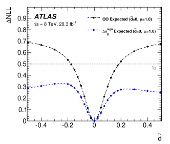
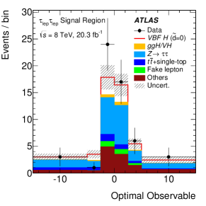
When we search for -violation in WBF Higgs production, the signed azimuthal angle between the tagging jets Plehn et al. (2002); Hankele et al. (2006), introduced in Sec. 6.3, is the appropriate genuine -odd observable. However, once we write down a model for -violation in the Higgs couplings to weak bosons, additional kinematic information from the form of the corresponding effective operators becomes available Brehmer et al. (2018a). We can write the optimal observable from Eq.(C.22) in terms of the SM and new physics matrix elements and find Aad et al. (2016f)
| (C.32) |
It allows us to extract the pre-factor of a -violating contribution to the coupling inducing the new physics amplitude . In Fig. 60 we show the corresponding ATLAS results based on lepton-lepton and lepton-hadron decays of WBF Higgs production with the subsequent decays . In the left panel we start with a comparison between the expected reach of the -odd observable and the optimal observable. Indeed, the latter is more sensitive on the dimension-6 realization of -violation. In the right panel we see the distribution for the signal and background events after a cut extracting the signal region through a boosted decision tree. The data peaks at small values of -odd contributions, with small tails expected from statistical and systematic uncertainties, indicating no sign of -violation in the weak gauge-Higgs sector.
Is it important to note that our toy model illustration of optimal observables does not imply that the Neyman-Pearson lemma is equivalent to the Cramér-Rao bound; the two statements are derived in different formalisms and with completely different assumptions. At parton level we can use the Neyman-Pearson lemma to systematically study the potential of a given analysis for separating two hypothesis, like for example to lead to a discovery of a specific signal in the presence of known backgrounds Cranmer and Plehn (2007). It is applied to actual searches through the matrix element method, described in Sec. 3.2. The Fisher information with the Cramér-Rao bound describes a continuous dependence on model parameters, allowing us to estimate the expected precision of any measurement in a combined signal and background sample. We illustrate the information geometry approach in Sec. 6.3 and generalize it to the detector-level in Sec. 3.3.
3.2 Matrix element method
Following a similar argument as for optimal observables, but for more general analysis tasks leads us to the matrix element method, which allows us to systematically include all relevant information from a signal phase space based on the Neyman–Pearson lemma. It states that the likelihood ratio is the most powerful test statistic to tell a simple null hypothesis — for example background only — from an alternate hypothesis — for example signal plus background. Here, maximum power is defined as the minimum probability for false negative error for a given probability of false positive. The key observation which relates this statement to LHC analyses is that the likelihood to populate a given phase space region given a model is nothing but the exclusive cross section as we use it in an event generator.
We start with a theoretical problem Cranmer and Plehn (2007), where we assume that we can ignore detector effects and have full control over the calculation of the differential cross section. In a counting experiment the likelihood of observing events in a given phase space region is given by a Poisson distribution. To describe phase space we introduce a observable , where we assume that the hypothesis is described by the normalized distribution , while the alternative hypothesis is described by . The single-event likelihood can then be factorized into the Poisson likelihood to observe an event and the normalized event likelihoods,
| (C.33) |
This expression replaces Eq.(C.19) from our toy model. Because the log-likelihood ratio is additive when we include more than one event or phase space configuration, we can integrate it the same way we integrate a differential cross section to a total or fiducial cross section. denotes the integrated luminosity. In Sec. 3.3 we will describe some ideas how to use the likelihood ratio directly in LHC analyses, while in this section we focus on ways to compute the phase-space dependence of the resulting statistical significance.
Because the log-likelihood ratio is the most powerful test statistics, we now generate a -distribution for events where we for example assume the hypothesis . We integrate over the entire phase space with the normalized event weight and generate the log-likelihood distributions
| (C.34) |
with a convolution in -space. Combining the log-likelihood distributions for and we can compute the maximum significance with which we will, assuming full control, be able to distinguish between two hypotheses at the LHC. Because the log-likelihood is additive we can apply the same method after integrating over part of phase space or after defining slices of phase space.
To illustrate this approach and its link to theory problems we show the maximum significance for the process
| (C.35) |
as discussed in Sec. 3, in Fig. 61. The individual bins are slices of the reconstructed , indicating that a slight boost of the decaying final state helps us to separate the signal from the continuum background. The drop towards large reflects the statistical limitation given by first term in Eq.(C.33) Plehn et al. (2014). Similar analyses are available for Higgs pair production, often used as a benchmark channel for the high-energy LHC or future hadron collidersKling et al. (2017); Gonçalves et al. (2018). As a tool on the Monte Carlo level, it allows us to model and understand the power of modern analysis methods in testing two theory hypotheses.
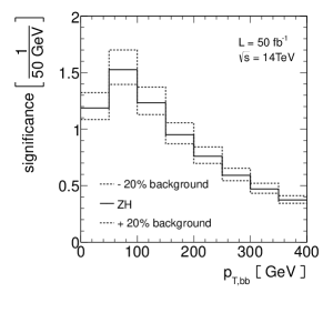
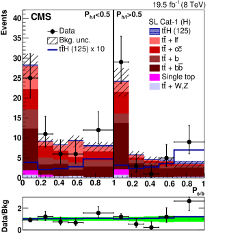
Whenever we want to extract a signal from a background at the LHC, we should be able to use the same test statistics for an actual number of events. This defines the matrix element method Kondo (1988); Abazov et al. (2004). Following Eq.(C.33), we need to compute the differential cross sections for the signal and background hypotheses for each event. There are three problems with this idea in practice:
A first, obvious problem arises if a background is reducible, so the signal and background phase spaces cannot be mapped onto each other to form the ratio for each event’s phase space point . To solve this problem, we have to integrate over the additional phase space direction given for example by an additional final state particle missed by the detector. Next, to compute the log-likelihood for the matrix element method we need to reconstruct the 4-momenta of all initial-state and final-state particles. While for leptons this seems feasible Gritsan et al. (2016), detector effects will lead to sizeable smearing in the corresponding 4-momentum. Even if by construction of the partonic 4-momenta in the hard process we manage to not violate energy and momentum conservation, detector effects turn the ratio into a ratio of integrals, not an integral of a ratio. Finally, when we compute perturbative QCD corrections involving virtual and real gluons we need to combine phase spaces with different number of final state particles Alwall et al. (2011). This can be solved by adapting the computation of the real emission diagrams Martini and Uwer (2015, 2018).
In principle, all of those problems can be overcome. One analysis where the matrix element method is applied in Higgs physics is the process Artoisenet et al. (2013b)
| (C.36) |
as discussed in Sec. 4. the notation represents a leptonic top decay. CMS has used the matrix element method in both the single lepton and the double lepton channel Khachatryan et al. (2015b), while ATLAS employed it in the single lepton channel as part of a larger set of input observables to a neural network Aad et al. (2015e). A major experimental challenge is how to include the -tagging in this analysis, so CMS actually uses two likelihood ratios, one describing the event kinematics and the other describing the heavy flavor content of the observed jets. In the right panel of Fig. 61 we show the log-likelihood ratio distribution measured by CMS, including the expected signal and background contribution. The left and right sets of curves clearly indicate the importance of -tagging in extracting the signal.
Just as a side remark, the input to the classic matrix element method are jets, possibly including tagging information. It is possible to extend the method to jet constituents, using the fact that Sudakov factors are nothing but no-splitting probabilities. This motivates the so-called shower deconstruction Soper and Spannowsky (2011, 2013, 2014).
3.3 Information geometry at detector level
In the last two section we have seen how likelihoods as a function of phase space and assuming a theory hypothesis are the central objects of modern analyses. However, in Higgs physics we want to reduce the focus on signal vs background analyses or simple observables and apply these ideas to measuring model parameters using the full log-likelihood information over the signal phase space. Such a model parameter dependence leads us to the idea of information geometry, usually defined in terms of the the Fisher information of Eq.(C.29) as the leading Taylor coefficient. It is not yet used in LHC analyses, but it is a standard approach for example in cosmological model tests and enjoys an obvious motivation in theoretical and experimental LHC physics; if we can compute the information geometry of LHC processes by extending the approach described in Sec.3.2 we gain full control over its link between LHC measurements and the physics we can extract from it Brehmer et al. (2017, 2018a).
One feature common to the optimal observables and matrix element method is that they are straightforward to implement at the Monte Carlo level, but that the description of detector effects is notoriously difficult. On the other hand, they need to be included because the likelihood ratio at parton level includes information which is not present at the detector level. The technical complication is that all steps from a parton-level phase space configuration to the measured 4-momenta in data, , are described by Markov processes; those cannot easily be inverted. It can be solved when we use the fact that these Markov processes are independent of the underlying theory hypothesis and . The detector-level equivalent to Eq.(C.33) reads
| (C.37) |
As long as the two hypotheses are irreducible, the full information on the hypotheses is included in the parton-level information , which can be easily computed with any event generator. The probability distribution describes the parton shower, detector resolution, and analysis requirements. They are modeled through a large set of random numbers, and they are not (easily) invertible.
One way to construct the ratio of the two event-level likelihoods is based on constructing proxies for -dependent distributions as -dependent distributions with the test function . We define this proxy nature by minimizing the specifically-chosen functional (or metric-like construction) Brehmer et al. (2018b)
| (C.38) |
The variational condition gives us the form of the proxy
| (C.39) |
One distribution we can approximate this way is the ratio of parton-level likelihoods from any event generator Brehmer et al. (2018b),
| (C.40) |
In this case, the input function is the parton-level likelihood ratio for each phase space point and does not even depend on . By numerically minimizing the corresponding version of Eq.(C.38) we can construct the observable-level likelihood ratio in Eq.(C.37).
When we compute likelihoods we do not only have access to likelihood values of individual phase space points, we can also treat the likelihood as a function over model space. This means that in our information geometry approach we can define the score as the vector of first derivatives
| (C.41) |
and find that the proxy for the parton-level score is the detector-level score,
| (C.42) |
To use the detector-level information geometry in practice, we need to minimize the functional first. This is a typical regression task for machine learning, where the to-be-minimized loss function will be inspired by the functional evaluated over all detector-level phase space points. This training of the detector-level likelihood ratio might take some time, but the usual advantage of the machine learning approach is that its evaluation will then be very fast.
While this construction focuses on the likelihood ratio, it is easily generalized to the Fisher information matrix defined in Eq.(C.29). The resulting information geometry, now including detector effects Brehmer et al. (2017, 2018a, 2018b), has the advantage that it defines a metric, which means that its results do not depend on the underlying parametrization. It allows us to study the parameter sensitivity from the entire phase space, parts of phase space, or slices in phase space independent of the model details. While this approach is an established way to analyze potential measurements at the Monte Carlo level, it has not yet been developed into an analysis strategy for the LHC.
3.4 Data-based machine learning
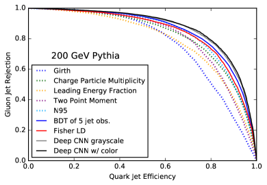
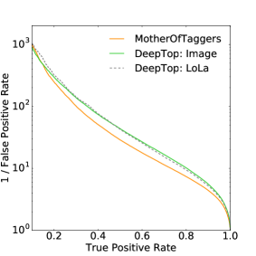
Machine learning techniques allow us to search for patterns in large amounts of highly complex data and has long been used by the LHC experiments. There, the number of events used in typical analyses is enormous, especially when we also consider the samples used to measure the detector performance and the background control regions. In addition, the LHC has a vast number of output channels for each event. This information is usually pre-processed into a number of theoretically well-defined observables. Multi-variate techniques working on a number of such high-level observables, including machine learning tools like neural networks, are standard in all Higgs analyses. The leading question in many Higgs analyses is why we rely on high-level observables as input to the neural networks describing the hard process, while we are happy to directly feed low-level detector output for example into a -tagging network. Given that many state-of-the-art LHC analyses only include a theory hypothesis in a full event simulation and then compare its output with data, this choice appears ad-hoc, and we have to ask ourselves if through our use of theory-motivated observables we lose information. Obviously, this ongoing paradigm change has profound implications for theoretical Higgs physics and the way we communicate between theory and experiment.
An example, where a loss of information from theory-motivated analysis objects motivates new analysis techniques, is subjet physics, introduced in Sec. 4. Analyses based on jet-level observables lose valuable information for example from hadronically decaying top quarks, and subjet tools made resonance searches in purely hadronic final state possible Aad et al. (2013). In terms of analysis objects this means that jets are no longer the main analysis objects in LHC analyses and merely separate the data into jet-level and subjet analyses. While on the theory side we are often struggling to analytically understand subjet observables beyond the leading-log approximation Dasgupta et al. (2013); Larkoski et al. (2017), this does not pose a problem for likelihood-free analyses. As long as we can simulate distinctive parton splitting patterns for signal and background processes, we do not have to define a quark or gluon to use this additional subjet information. As usual, high-level observables described by Feynman diagrams for the hard process mostly serve as an illustration.
Rapid progress in machine learning outside particle physics have paved the way to systematically search for patterns based on a large set of low-level observables, rather than a limited number of high-level observables. This development is at the heart of machine learning at the LHC, where we try to identify analyses where a multi-variate analysis of high-level observables might miss information Komiske et al. (2018). For such cases, machine learning tools will extract this information from low-level detector information. Given the success of subjet physics and the curious attitude in that field, an obvious question is how much we can improve the performance of established multi-variate subjet analyses Kasieczka et al. (2015); Luo et al. (2017) by using low-level input and machine learning. To participate in the advances of machine learning outside particle physics we organize the experimental information in a standardized manner. We then train a neural network on some combination of data and simulation, ideally with a cross entropy loss function, such that the output can be interpreted as a probability for an underlying hypothesis. This probability can be viewed as the final outcome or as input to another analysis, for instance going from jets to full events. The first proposed subjet analyses using machine learning are calorimeter images evaluated with convolutional networks Cogan et al. (2015); de Oliveira et al. (2016); Baldi et al. (2016); Barnard et al. (2017); Kasieczka et al. (2017); Macaluso and Shih (2018). Calorimeter images are 2-dimensional heat maps, encoding the energy deposition in the rapidity vs azimuthal angle plane. The main problem with the image approach is the combination of calorimeter and tracking information, because the two sets of low-level data have a very different resolution. In the left panel of Fig. 62 we show a comparison of a convolutional network using the combined calorimeter and tracking information with high-level observables Komiske et al. (2017). A similar picture arises when we compare low-level machine learning and high-level multi-variate top taggers Kasieczka et al. (2017); Macaluso and Shih (2018): machine learning methods based on low-level inputs can do better than the best high-level multi-variate analyses.
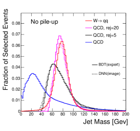
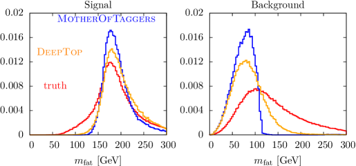
Image recognition is not the only active field in machine learning. Alternatively, we can buy into new ideas in natural language recognition and apply them to subjet analyses Louppe et al. (2017); Cheng (2017). Finally, we can derive inspiration on the data input format from physics, for instance organizing the measured energy and momentum of a particle in terms of 4-vectors Almeida et al. (2015); Pearkes et al. (2017) and either using or learning the Minkowski metric Butter et al. (2017). We compare the performance of an image-based top tagger and a 4-vector-based top tagger with identical training samples in the right panel of Fig. 62. The question of which low-level input format is the most appropriate for subjet analyses is complicated by the fact that eventually we need to include information on displaced vertices or leptons, similar to heavy-flavor taggers.
To illustrate how we can understand the performance of machine learning techniques applied to low-level observables we show the jet mass distribution for an image-based -tagger Baldi et al. (2016) and top tagger Kasieczka et al. (2017) in Fig. 63. In both cases we compare the Monte Carlo truth level with a BDT analysis and the convolutional network result. For the -tagger we can clearly see how a stiffer background rejection drives the distribution towards the generated signal. For the top tagger we show correctly identified signal and background events and compare them with the Monte Carlo truth. The BDT with the jet mass as one of its inputs clearly separates the corresponding events, whereas the neural network also identifies events with a less clear separation in jet mass. Such events frequently appear in the simulated data. These examples illustrate how we can understand the classification through a neural network in terms of first-principles observables at least as well as we control a BDT acting on high-level inputs. The neural network is not a blacker box than a BDT acting on a large correlated set of high-level observables.
Analyzing whole events using machine learning based on high-level observables is an established analysis strategy. One problem with this technique is that the relevant signal regions in phase space might be plagued with large systematic or theoretical uncertainties, which have to be implemented by hand. If these uncertainties are part of the even simulation, we can include them in the spirit of comparing full simulations to data by using adversarial networks Louppe et al. (2016). The role of the process
| (C.43) |
with a moderately boosted Higgs boson and up to two jets has been discussed in detail in Sec. 1.4. The final state at the jet level can be described by a small number of high-level kinematics observables, like the transverse momentum of the Higgs or the jets, their rapidities, or their azimuthal angle separations. Of these variables the transverse momentum of the leading jet carries information about the nature of the hard interaction. The size of the corresponding tails of the distribution requires us to understand the bulk of the distribution, or the total production rate. The latter, however, is affected by perturbative uncertainties, which can be described in terms of scale choices in the event generation. This allows us to use a set of adversarial networks, where the role of the adversary is to remove all information that can be covered by the scale choice Englert et al. (2018). In the left panel of Fig. 64 we show the output of the adversarial network, comparing the signal including a dimension-6 contribution to the Higgs-gluon interaction with the top-induced Standard Model prediction. The Standard Model simulations with different scale choices, and hence significantly different total rates, all score essentially the same, while the dimension-6 signal shows a clear preference of a large neural network score.
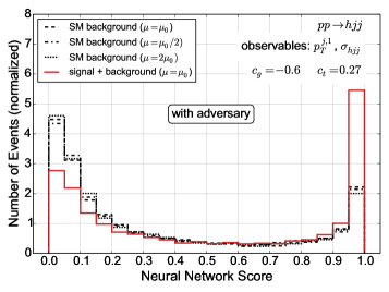
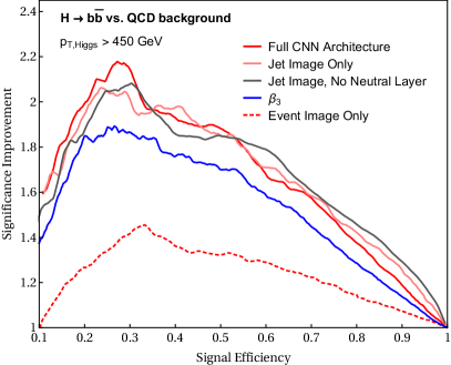
Moving beyond the high-level observables altogether, the ultimate goal in machine learning at the LHC is to analyze entire events based on low-level observables at the subjet-level and on the jet level. Instead of generalizing subjet applications to the full calorimeter and tracker coverage, it is convenient to separate events into jet-level and subjet information. This can be studied for boosted Higgs production Lin et al. (2018),
| (C.44) |
The physics aspects of this process are discussed in Sec. 1.4. Standard resonance search methods have not been successful for such an all-hadronic channel due to the overwhelming jet backgrounds. In the boosted configuration, the two -jets are close to each other and can be identified using subjet methods, pioneered in Higgs physics by Ref. Butterworth et al. (2008). First, the role of the Higgs tagger can obviously been played by a convolutional network acting on jet images. It will identify the Higgs decay through a high-resolution jet image with pixels. For now, a double -tag inside the candidate Higgs jet is required in addition to the low-level calorimeter information. A second convolutional network searches for jet-like features in a coarser pixels image of the entire event. The periodic boundary conditions are included through pre-processing and the network setup. This second image does not resolve subjet structures, but it is of the same order as the typical calorimeter resolution for jet-level objects. This way, it probes the kinematic correlations between the Higgs jet and the other even features. For the specific +jets signal the main physics question then becomes how much information we can extract from the number of recoil jets and their kinematics. In the right panel of Fig. 64 we show the improvement of the dual network analysis over a simple kinematic analysis. We see how the impact of the jet-level network is significantly exceeded by the subjet-level network, clearly making the case that a combination of the two analysis tools should be the ATLAS and CMS default for the coming LHC runs.
D Conclusions
With the discovery of the Higgs boson in 2012 the Standard Model withstood its ultimate test. Our understanding of perturbative quantum field theory has been fully validated. The Standard Model is a sophisticated theory that pulls out all the stops of our field theory toolbox to make sense of an enormous amount of data. We detailed this in this review in various contexts, and it would have been easy to find even more praise for the Standard Model as an incredibly successful theory. But this would obscure a more relevant point. The task of particle physics post Higgs discovery is a different one. The Standard Model — been there, done that, wore the T-shirt. So what lies beyond?
While high energy physicists are well aware of the philosophical and practical limitations of the Standard Model, the blessing that is its renormalizable character which underpins its discovery based on a precise quantum analysis of its interactions has also become its curse. Past discoveries like the top quark or the Higgs boson itself were anticipated. If these fields had not been discovered this would have challenged our otherwise successful understanding of quantum field theory. In this sense, the Higgs discovery was not at all a coincidence but the pinnacle of a well thought-out plan, which would have had a positive scientific outcome even in the absence of a discovery.
However, some six years after the Higgs boson discovery, the sidewalk has apparently come to an end. On the one hand, all motivated and established perturbative UV-complete theories that seek to embed the Higgs into a more fundamental picture of the TeV scale stand challenged. On the other hand, strongly-interacting approaches to the electroweak scale lack experimental motivation and often push our perturbative QFT toolbox over the edge. This makes concrete predictions hard to obtain, while first-principle lattice calculations will require more time to catch up. Adding the so-far negative outcome of searches for new physics of any kind at the LHC to the mix, one could develop a rather bleak outlook on particle physics and Higgs phenomenology in particular.
But Higgs ain’t over till it’s over. The past years have seen tremendous progress and success in both experimental and theoretical particle physics, and most importantly at the intersection of both communities. While precision and interpretation approaches based on effective field theory or concrete UV-complete models are continually pushed forward, novel analyses and search strategies that rely on the combined expertise of experimentalists and theorists have shaped the LHC’s phenomenology program like no other collider experiment before. Hadron colliders have been transformed from the historic discovery machines to a comprehensive precision physics program.
The Higgs boson, as the central part of electroweak symmetry breaking, is typically considered as a harbinger of an even more satisfactory UV theory of particle physics that contains the Standard Model and stands at the center of this development. Novel approaches, which build on insights ranging from advanced data-analysis all the way to a better understanding of the theoretical background of sensitivity-limiting factors will set the scope of a Higgs precision program that is likely to surpass earlier expectations. It is therefore realistic to expect a significant improvement of the current Higgs property measurements as well as Higgs exotic searches. Together they provide a coherent approach to understanding the nature of the electroweak scale and its place in the physics landscape. Theoretical progress in the precise prediction of new physics phenomena (e.g. in the MSSM or 2HDMs), as well as the interpretation of data in a largely model-independent way on the grounds of EFT is now met by experimentally sophisticated techniques to extract information about the Higgs boson in its rarest final states even at comparably low statistics. This will (hopefully) enable discoveries of as yet unanticipated phenomena. The aim of this review is to bridge the basic ideas that have motivated decades of research to these recent developments.
Acknowledgments
First, we would like to thank all our collaborators on many fun Higgs projects over the years and everyone who went through this review and reminded us of mistakes and shortcomings, explicitly mentioning Michael Spira. C.E. and T.P. thank Peter Zerwas for introducing them to the topic. We are grateful to the Mainz Institute for Theoretical Physics for its hospitality. T.P. and C.E. are grateful to TASI 2018, where parts of this review were finalized. S.D. is supported by the U.S. Department of Energy under Grant Contract de-sc0012704. C.E. is supported by the IPPP Associateship scheme and by the UK Science and Technology Facilities Council (STFC) under grant ST/P000746/1.
References
- Higgs (1964a) P. W. Higgs, Phys. Rev. Lett. 13, 508 (1964a), [160(1964)].
- Higgs (1964b) P. W. Higgs, Phys. Lett. 12, 132 (1964b).
- Englert and Brout (1964) F. Englert and R. Brout, Phys. Rev. Lett. 13, 321 (1964), [157(1964)].
- Guralnik et al. (1964) G. S. Guralnik, C. R. Hagen, and T. W. B. Kibble, Phys. Rev. Lett. 13, 585 (1964), [162(1964)].
- Kibble (1967) T. W. B. Kibble, Phys. Rev. 155, 1554 (1967), [165(1967)].
- Higgs (1966) P. W. Higgs, Phys. Rev. 145, 1156 (1966).
- Chatrchyan et al. (2012) S. Chatrchyan et al. (CMS), Science 338, 1569 (2012).
- Aad et al. (2012) G. Aad et al. (ATLAS), Phys. Lett. B716, 1 (2012), arXiv:1207.7214 [hep-ex].
- Aad et al. (2015a) G. Aad et al. (ATLAS, CMS), Phys. Rev. Lett. 114, 191803 (2015a), arXiv:1503.07589 [hep-ex].
- Fermi (1934) E. Fermi, Z. Phys. 88, 161 (1934).
- Anderson (1963) P. W. Anderson, Phys. Rev. 130, 439 (1963), [153(1963)].
- Fujikawa et al. (1972) K. Fujikawa, B. W. Lee, and A. I. Sanda, Phys. Rev. D6, 2923 (1972).
- Becchi et al. (1974) C. Becchi, A. Rouet, and R. Stora, Phys. Lett. 52B, 344 (1974).
- Becchi et al. (1975) C. Becchi, A. Rouet, and R. Stora, Commun. Math. Phys. 42, 127 (1975).
- Becchi et al. (1976) C. Becchi, A. Rouet, and R. Stora, Annals Phys. 98, 287 (1976).
- Tyutin (1975) I. V. Tyutin, (1975), arXiv:0812.0580 [hep-th].
- ’t Hooft (1994) G. ’t Hooft, Adv. Ser. Math. Phys. 19, 1 (1994).
- Weinberg (1960) S. Weinberg, Phys. Rev. 118, 838 (1960).
- ’t Hooft and Veltman (1972) G. ’t Hooft and M. J. G. Veltman, Nucl. Phys. B44, 189 (1972).
- Goldstone (1961) J. Goldstone, Nuovo Cim. 19, 154 (1961).
- Glashow (1961) S. L. Glashow, Nucl. Phys. 22, 579 (1961).
- Salam and Ward (1964) A. Salam and J. C. Ward, Phys. Lett. 13, 168 (1964).
- Weinberg (1967a) S. Weinberg, Phys. Rev. Lett. 19, 1264 (1967a).
- Goldstone et al. (1962) J. Goldstone, A. Salam, and S. Weinberg, Phys. Rev. 127, 965 (1962).
- Romao and Silva (2012) J. C. Romao and J. P. Silva, Int. J. Mod. Phys. A27, 1230025 (2012), arXiv:1209.6213 [hep-ph].
- Bjorken and Weinberg (1977) J. D. Bjorken and S. Weinberg, Phys. Rev. Lett. 38, 622 (1977).
- Barr and Zee (1990) S. M. Barr and A. Zee, Phys. Rev. Lett. 65, 21 (1990), [Erratum: Phys. Rev. Lett.65,2920(1990)].
- Degrassi et al. (1991) G. Degrassi, S. Fanchiotti, and A. Sirlin, Nucl. Phys. B351, 49 (1991).
- Haller et al. (2018) J. Haller, A. Hoecker, R. Kogler, K. Mönig, T. Peiffer, and J. Stelzer, (2018), arXiv:1803.01853 [hep-ph].
- Schael et al. (2006) S. Schael et al. (SLD Electroweak Group, DELPHI, ALEPH, SLD, SLD Heavy Flavour Group, OPAL, LEP Electroweak Working Group, L3), Phys. Rept. 427, 257 (2006), arXiv:hep-ex/0509008 [hep-ex].
- Peskin and Takeuchi (1990) M. E. Peskin and T. Takeuchi, Phys. Rev. Lett. 65, 964 (1990).
- Peskin and Takeuchi (1992) M. E. Peskin and T. Takeuchi, Phys. Rev. D46, 381 (1992).
- Altarelli and Barbieri (1991) G. Altarelli and R. Barbieri, Phys. Lett. B253, 161 (1991).
- Bardin et al. (2001) D. Yu. Bardin, P. Christova, M. Jack, L. Kalinovskaya, A. Olchevski, S. Riemann, and T. Riemann, Comput. Phys. Commun. 133, 229 (2001), arXiv:hep-ph/9908433 [hep-ph].
- de Blas et al. (2016) J. de Blas, M. Ciuchini, E. Franco, S. Mishima, M. Pierini, L. Reina, and L. Silvestrini, JHEP 12, 135 (2016), arXiv:1608.01509 [hep-ph].
- Dittmaier et al. (2011) S. Dittmaier et al. (LHC Higgs Cross Section Working Group), (2011), 10.5170/CERN-2011-002, arXiv:1101.0593 [hep-ph].
- de Florian et al. (2016a) D. de Florian et al. (LHC Higgs Cross Section Working Group), (2016a), 10.23731/CYRM-2017-002, arXiv:1610.07922 [hep-ph].
- Gunion et al. (2000) J. F. Gunion, H. E. Haber, G. L. Kane, and S. Dawson, Front. Phys. 80, 1 (2000).
- Djouadi (2008) A. Djouadi, Phys. Rept. 457, 1 (2008), arXiv:hep-ph/0503172 [hep-ph].
- Spira (2017) M. Spira, Prog. Part. Nucl. Phys. 95, 98 (2017), arXiv:1612.07651 [hep-ph].
- Djouadi et al. (1998) A. Djouadi, J. Kalinowski, and M. Spira, Comput. Phys. Commun. 108, 56 (1998), arXiv:hep-ph/9704448 [hep-ph].
- Djouadi et al. (2018) A. Djouadi, J. Kalinowski, M. Muehlleitner, and M. Spira, (2018), arXiv:1801.09506 [hep-ph].
- Bredenstein et al. (2007) A. Bredenstein, A. Denner, S. Dittmaier, and M. M. Weber (2007) pp. 150–154, arXiv:0708.4123 [hep-ph].
- Drees and Hikasa (1990) M. Drees and K.-i. Hikasa, Phys. Lett. B240, 455 (1990), [Erratum: Phys. Lett.B262,497(1991)].
- Braaten and Leveille (1980) E. Braaten and J. P. Leveille, Phys. Rev. D22, 715 (1980).
- Dabelstein and Hollik (1992) A. Dabelstein and W. Hollik, Z. Phys. C53, 507 (1992).
- Kniehl (1994) B. A. Kniehl, Phys. Rept. 240, 211 (1994).
- Rizzo (1980) T. G. Rizzo, Phys. Rev. D22, 722 (1980).
- Keung and Marciano (1984) W.-Y. Keung and W. J. Marciano, Phys. Rev. D30, 248 (1984).
- Georgi et al. (1978) H. M. Georgi, S. L. Glashow, M. E. Machacek, and D. V. Nanopoulos, Phys. Rev. Lett. 40, 692 (1978).
- Ellis et al. (1979) J. R. Ellis, M. K. Gaillard, D. V. Nanopoulos, and C. T. Sachrajda, Phys. Lett. 83B, 339 (1979).
- Baikov and Chetyrkin (2006) P. A. Baikov and K. G. Chetyrkin, Phys. Rev. Lett. 97, 061803 (2006), arXiv:hep-ph/0604194 [hep-ph].
- Appelquist and Carazzone (1975) T. Appelquist and J. Carazzone, Phys. Rev. D11, 2856 (1975).
- Kribs et al. (2007) G. D. Kribs, T. Plehn, M. Spannowsky, and T. M. P. Tait, Phys. Rev. D76, 075016 (2007), arXiv:0706.3718 [hep-ph].
- Denner et al. (2012a) A. Denner, S. Dittmaier, A. Muck, G. Passarino, M. Spira, C. Sturm, S. Uccirati, and M. M. Weber, Eur. Phys. J. C72, 1992 (2012a), arXiv:1111.6395 [hep-ph].
- Eberhardt et al. (2012) O. Eberhardt, G. Herbert, H. Lacker, A. Lenz, A. Menzel, U. Nierste, and M. Wiebusch, Phys. Rev. Lett. 109, 241802 (2012), arXiv:1209.1101 [hep-ph].
- Denner et al. (2011) A. Denner, S. Heinemeyer, I. Puljak, D. Rebuzzi, and M. Spira, Eur. Phys. J. C71, 1753 (2011), arXiv:1107.5909 [hep-ph].
- Ellis et al. (1976) J. R. Ellis, M. K. Gaillard, and D. V. Nanopoulos, Nucl. Phys. B106, 292 (1976).
- Plehn (2012) T. Plehn, Lect. Notes Phys. 844, 1 (2012), arXiv:0910.4182 [hep-ph].
- Cahn et al. (1979) R. N. Cahn, M. S. Chanowitz, and N. Fleishon, Phys. Lett. 82B, 113 (1979).
- Bergstrom and Hulth (1985) L. Bergstrom and G. Hulth, Nucl. Phys. B259, 137 (1985), [Erratum: Nucl. Phys.B276,744(1986)].
- Froggatt and Nielsen (1979) C. D. Froggatt and H. B. Nielsen, Nucl. Phys. B147, 277 (1979).
- Giudice and Lebedev (2008) G. F. Giudice and O. Lebedev, Phys. Lett. B665, 79 (2008), arXiv:0804.1753 [hep-ph].
- Alte et al. (2016) S. Alte, M. König, and M. Neubert, JHEP 12, 037 (2016), arXiv:1609.06310 [hep-ph].
- Bodwin et al. (2013) G. T. Bodwin, F. Petriello, S. Stoynev, and M. Velasco, Phys. Rev. D88, 053003 (2013), arXiv:1306.5770 [hep-ph].
- Bodwin et al. (2014) G. T. Bodwin, H. S. Chung, J.-H. Ee, J. Lee, and F. Petriello, Phys. Rev. D90, 113010 (2014), arXiv:1407.6695 [hep-ph].
- König and Neubert (2015) M. König and M. Neubert, JHEP 08, 012 (2015), arXiv:1505.03870 [hep-ph].
- Bhattacharya et al. (2014) B. Bhattacharya, A. Datta, and D. London, Phys. Lett. B736, 421 (2014), arXiv:1407.0695 [hep-ph].
- Chatrchyan et al. (2013a) S. Chatrchyan et al. (CMS), Phys. Lett. B726, 587 (2013a), arXiv:1307.5515 [hep-ex].
- Andersen et al. (2013) J. R. Andersen et al. (LHC Higgs Cross Section Working Group), (2013), 10.5170/CERN-2013-004, arXiv:1307.1347 [hep-ph].
- Doršner et al. (2015) I. Doršner, S. Fajfer, A. Greljo, J. F. Kamenik, N. Košnik, and I. Nišandžic, JHEP 06, 108 (2015), arXiv:1502.07784 [hep-ph].
- Arganda et al. (2005) E. Arganda, A. M. Curiel, M. J. Herrero, and D. Temes, Phys. Rev. D71, 035011 (2005), arXiv:hep-ph/0407302 [hep-ph].
- Llewellyn Smith (1973) C. H. Llewellyn Smith, Phys. Lett. 46B, 233 (1973).
- Cornwall et al. (1974) J. M. Cornwall, D. N. Levin, and G. Tiktopoulos, Phys. Rev. D10, 1145 (1974), [Erratum: Phys. Rev.D11,972(1975)].
- Lee et al. (1977a) B. W. Lee, C. Quigg, and H. B. Thacker, Phys. Rev. Lett. 38, 883 (1977a).
- Lee et al. (1977b) B. W. Lee, C. Quigg, and H. B. Thacker, Phys. Rev. D16, 1519 (1977b).
- Chanowitz et al. (1978) M. S. Chanowitz, M. A. Furman, and I. Hinchliffe, Phys. Lett. 78B, 285 (1978).
- Chanowitz et al. (1979) M. S. Chanowitz, M. A. Furman, and I. Hinchliffe, Nucl. Phys. B153, 402 (1979).
- Buttazzo et al. (2013) D. Buttazzo, G. Degrassi, P. P. Giardino, G. F. Giudice, F. Sala, A. Salvio, and A. Strumia, JHEP 12, 089 (2013), arXiv:1307.3536 [hep-ph].
- Eichhorn et al. (2015) A. Eichhorn, H. Gies, J. Jaeckel, T. Plehn, M. M. Scherer, and R. Sondenheimer, JHEP 04, 022 (2015), arXiv:1501.02812 [hep-ph].
- Maiani et al. (1978) L. Maiani, G. Parisi, and R. Petronzio, Nucl. Phys. B136, 115 (1978).
- Dashen and Neuberger (1983) R. F. Dashen and H. Neuberger, Phys. Rev. Lett. 50, 1897 (1983).
- Lindner (1986) M. Lindner, Z. Phys. C31, 295 (1986).
- Krive and Linde (1976) I. V. Krive and A. D. Linde, Nucl. Phys. B117, 265 (1976).
- Krasnikov (1978) N. V. Krasnikov, Yad. Fiz. 28, 549 (1978).
- Lindner et al. (1989) M. Lindner, M. Sher, and H. W. Zaglauer, Phys. Lett. B228, 139 (1989).
- Sher (1989) M. Sher, Phys. Rept. 179, 273 (1989).
- Holland (2005) K. Holland, Lattice field theory. Proceedings, 22nd International Symposium, Lattice 2004, Batavia, USA, June 21-26, 2004, Nucl. Phys. Proc. Suppl. 140, 155 (2005), [155(2004)], arXiv:hep-lat/0409112 [hep-lat].
- Schrempp and Wimmer (1996) B. Schrempp and M. Wimmer, Prog. Part. Nucl. Phys. 37, 1 (1996), arXiv:hep-ph/9606386 [hep-ph].
- Pendleton and Ross (1981) B. Pendleton and G. G. Ross, Phys. Lett. 98B, 291 (1981).
- Hill (1981) C. T. Hill, Phys. Rev. D24, 691 (1981).
- Wetterich (1981) C. Wetterich, Phys. Lett. 104B, 269 (1981).
- Shaposhnikov and Wetterich (2010) M. Shaposhnikov and C. Wetterich, Phys. Lett. B683, 196 (2010), arXiv:0912.0208 [hep-th].
- Sakharov (1967) A. D. Sakharov, Pisma Zh. Eksp. Teor. Fiz. 5, 32 (1967), [Usp. Fiz. Nauk161,no.5,61(1991)].
- Grojean et al. (2005) C. Grojean, G. Servant, and J. D. Wells, Phys. Rev. D71, 036001 (2005), arXiv:hep-ph/0407019 [hep-ph].
- Reichert et al. (2018) M. Reichert, A. Eichhorn, H. Gies, J. M. Pawlowski, T. Plehn, and M. M. Scherer, Phys. Rev. D97, 075008 (2018), arXiv:1711.00019 [hep-ph].
- Profumo et al. (2015) S. Profumo, M. J. Ramsey-Musolf, C. L. Wainwright, and P. Winslow, Phys. Rev. D91, 035018 (2015), arXiv:1407.5342 [hep-ph].
- Kurup and Perelstein (2017) G. Kurup and M. Perelstein, Phys. Rev. D96, 015036 (2017), arXiv:1704.03381 [hep-ph].
- Chen et al. (2017) C.-Y. Chen, J. Kozaczuk, and I. M. Lewis, JHEP 08, 096 (2017), arXiv:1704.05844 [hep-ph].
- Chiang et al. (2018) C.-W. Chiang, M. J. Ramsey-Musolf, and E. Senaha, Phys. Rev. D97, 015005 (2018), arXiv:1707.09960 [hep-ph].
- Basler et al. (2018) P. Basler, M. Mühlleitner, and J. Wittbrodt, JHEP 03, 061 (2018), arXiv:1711.04097 [hep-ph].
- Dunne and Unsal (2012) G. V. Dunne and M. Unsal, JHEP 11, 170 (2012), arXiv:1210.2423 [hep-th].
- Langacker (1981) P. Langacker, Phys. Rept. 72, 185 (1981).
- Chen et al. (2006) M.-C. Chen, S. Dawson, and T. Krupovnickas, Phys. Rev. D74, 035001 (2006), arXiv:hep-ph/0604102 [hep-ph].
- Cheng et al. (1974) T. P. Cheng, E. Eichten, and L.-F. Li, Phys. Rev. D9, 2259 (1974).
- Barger et al. (2009) V. Barger, H. E. Logan, and G. Shaughnessy, Phys. Rev. D79, 115018 (2009), arXiv:0902.0170 [hep-ph].
- Silveira and Zee (1985) V. Silveira and A. Zee, Phys. Lett. 161B, 136 (1985).
- O’Connell et al. (2007) D. O’Connell, M. J. Ramsey-Musolf, and M. B. Wise, Phys. Rev. D75, 037701 (2007), arXiv:hep-ph/0611014 [hep-ph].
- Bowen et al. (2007) M. Bowen, Y. Cui, and J. D. Wells, JHEP 03, 036 (2007), arXiv:hep-ph/0701035 [hep-ph].
- Pruna and Robens (2013) G. M. Pruna and T. Robens, Phys. Rev. D88, 115012 (2013), arXiv:1303.1150 [hep-ph].
- Espinosa et al. (2012) J. R. Espinosa, T. Konstandin, and F. Riva, Nucl. Phys. B854, 592 (2012), arXiv:1107.5441 [hep-ph].
- Dawson and Lewis (2015) S. Dawson and I. M. Lewis, Phys. Rev. D92, 094023 (2015), arXiv:1508.05397 [hep-ph].
- Chen et al. (2015a) C.-Y. Chen, S. Dawson, and I. M. Lewis, Phys. Rev. D91, 035015 (2015a), arXiv:1410.5488 [hep-ph].
- López-Val et al. (2013) D. López-Val, T. Plehn, and M. Rauch, JHEP 10, 134 (2013), arXiv:1308.1979 [hep-ph].
- McDonald (1994) J. McDonald, Phys. Rev. D50, 3637 (1994), arXiv:hep-ph/0702143 [HEP-PH].
- Burgess et al. (2001) C. P. Burgess, M. Pospelov, and T. ter Veldhuis, Nucl. Phys. B619, 709 (2001), arXiv:hep-ph/0011335 [hep-ph].
- Binoth and van der Bij (1997) T. Binoth and J. J. van der Bij, Z. Phys. C75, 17 (1997), arXiv:hep-ph/9608245 [hep-ph].
- Schabinger and Wells (2005) R. M. Schabinger and J. D. Wells, Phys. Rev. D72, 093007 (2005), arXiv:hep-ph/0509209 [hep-ph].
- Patt and Wilczek (2006) B. Patt and F. Wilczek, (2006), arXiv:hep-ph/0605188 [hep-ph].
- Lebedev et al. (2012) O. Lebedev, H. M. Lee, and Y. Mambrini, Phys. Lett. B707, 570 (2012), arXiv:1111.4482 [hep-ph].
- Shifman et al. (1978) M. A. Shifman, A. I. Vainshtein, and V. I. Zakharov, Phys. Lett. 78B, 443 (1978).
- Shrock and Suzuki (1982) R. E. Shrock and M. Suzuki, Phys. Lett. 110B, 250 (1982).
- Arcadi et al. (2018) G. Arcadi, M. Dutra, P. Ghosh, M. Lindner, Y. Mambrini, M. Pierre, S. Profumo, and F. S. Queiroz, Eur. Phys. J. C78, 203 (2018), arXiv:1703.07364 [hep-ph].
- Haber et al. (1979) H. E. Haber, G. L. Kane, and T. Sterling, Nucl. Phys. B161, 493 (1979).
- Branco et al. (2012) G. C. Branco, P. M. Ferreira, L. Lavoura, M. N. Rebelo, M. Sher, and J. P. Silva, Phys. Rept. 516, 1 (2012), arXiv:1106.0034 [hep-ph].
- Gunion and Haber (2005) J. F. Gunion and H. E. Haber, Phys. Rev. D72, 095002 (2005), arXiv:hep-ph/0506227 [hep-ph].
- Ma (2006) E. Ma, Phys. Rev. D73, 077301 (2006), arXiv:hep-ph/0601225 [hep-ph].
- Cline et al. (1996) J. M. Cline, K. Kainulainen, and A. P. Vischer, Phys. Rev. D54, 2451 (1996), arXiv:hep-ph/9506284 [hep-ph].
- Fromme et al. (2006) L. Fromme, S. J. Huber, and M. Seniuch, JHEP 11, 038 (2006), arXiv:hep-ph/0605242 [hep-ph].
- Gong et al. (2012) J.-O. Gong, H. M. Lee, and S. K. Kang, JHEP 04, 128 (2012), arXiv:1202.0288 [hep-ph].
- Pilaftsis and Wagner (1999) A. Pilaftsis and C. E. M. Wagner, Nucl. Phys. B553, 3 (1999), arXiv:hep-ph/9902371 [hep-ph].
- Gunion and Haber (2003) J. F. Gunion and H. E. Haber, Phys. Rev. D67, 075019 (2003), arXiv:hep-ph/0207010 [hep-ph].
- Kanemura et al. (1999) S. Kanemura, T. Kasai, and Y. Okada, Phys. Lett. B471, 182 (1999), arXiv:hep-ph/9903289 [hep-ph].
- Craig et al. (2015) N. Craig, F. D’Eramo, P. Draper, S. Thomas, and H. Zhang, JHEP 06, 137 (2015), arXiv:1504.04630 [hep-ph].
- Carena et al. (2014) M. Carena, I. Low, N. R. Shah, and C. E. M. Wagner, JHEP 04, 015 (2014), arXiv:1310.2248 [hep-ph].
- Bhupal Dev and Pilaftsis (2014) P. S. Bhupal Dev and A. Pilaftsis, JHEP 12, 024 (2014), [Erratum: JHEP11,147(2015)], arXiv:1408.3405 [hep-ph].
- Battye et al. (2011) R. A. Battye, G. D. Brawn, and A. Pilaftsis, JHEP 08, 020 (2011), arXiv:1106.3482 [hep-ph].
- Pilaftsis (2012) A. Pilaftsis, Phys. Lett. B706, 465 (2012), arXiv:1109.3787 [hep-ph].
- He et al. (2001) H.-J. He, N. Polonsky, and S.-f. Su, Phys. Rev. D64, 053004 (2001), arXiv:hep-ph/0102144 [hep-ph].
- Hall and Wise (1981) L. J. Hall and M. B. Wise, Nucl. Phys. B187, 397 (1981).
- Glashow and Weinberg (1977) S. L. Glashow and S. Weinberg, Phys. Rev. D15, 1958 (1977).
- D’Ambrosio et al. (2002) G. D’Ambrosio, G. F. Giudice, G. Isidori, and A. Strumia, Nucl. Phys. B645, 155 (2002), arXiv:hep-ph/0207036 [hep-ph].
- Dery et al. (2013) A. Dery, A. Efrati, G. Hiller, Y. Hochberg, and Y. Nir, JHEP 08, 006 (2013), arXiv:1304.6727 [hep-ph].
- Pich and Tuzon (2009) A. Pich and P. Tuzon, Phys. Rev. D80, 091702 (2009), arXiv:0908.1554 [hep-ph].
- Davidson and Haber (2005) S. Davidson and H. E. Haber, Phys. Rev. D72, 035004 (2005), [Erratum: Phys. Rev.D72,099902(2005)], arXiv:hep-ph/0504050 [hep-ph].
- Eriksson et al. (2010) D. Eriksson, J. Rathsman, and O. Stal, Comput. Phys. Commun. 181, 189 (2010), arXiv:0902.0851 [hep-ph].
- Casalbuoni et al. (1986) R. Casalbuoni, D. Dominici, R. Gatto, and C. Giunti, Phys. Lett. B178, 235 (1986).
- Casalbuoni et al. (1988) R. Casalbuoni, D. Dominici, F. Feruglio, and R. Gatto, Nucl. Phys. B299, 117 (1988).
- Kanemura et al. (1993) S. Kanemura, T. Kubota, and E. Takasugi, Phys. Lett. B313, 155 (1993), arXiv:hep-ph/9303263 [hep-ph].
- Akeroyd et al. (2000) A. G. Akeroyd, A. Arhrib, and E.-M. Naimi, Phys. Lett. B490, 119 (2000), arXiv:hep-ph/0006035 [hep-ph].
- Ginzburg and Ivanov (2005) I. F. Ginzburg and I. P. Ivanov, Phys. Rev. D72, 115010 (2005), arXiv:hep-ph/0508020 [hep-ph].
- Osland et al. (2008) P. Osland, P. N. Pandita, and L. Selbuz, Phys. Rev. D78, 015003 (2008), arXiv:0802.0060 [hep-ph].
- Cornwall et al. (1973) J. M. Cornwall, D. N. Levin, and G. Tiktopoulos, Phys. Rev. Lett. 30, 1268 (1973), [Erratum: Phys. Rev. Lett.31,572(1973)].
- Weldon (1984) H. A. Weldon, Phys. Rev. D30, 1547 (1984).
- Gunion et al. (1991a) J. F. Gunion, H. E. Haber, and J. Wudka, Phys. Rev. D43, 904 (1991a).
- Chen and Dawson (2013) C.-Y. Chen and S. Dawson, Phys. Rev. D87, 055016 (2013), arXiv:1301.0309 [hep-ph].
- Deshpande and Ma (1978) N. G. Deshpande and E. Ma, Phys. Rev. D18, 2574 (1978).
- Majumdar and Ghosal (2008) D. Majumdar and A. Ghosal, Mod. Phys. Lett. A23, 2011 (2008), arXiv:hep-ph/0607067 [hep-ph].
- Barbieri et al. (2006) R. Barbieri, L. J. Hall, and V. S. Rychkov, Phys. Rev. D74, 015007 (2006), arXiv:hep-ph/0603188 [hep-ph].
- Lopez Honorez et al. (2007) L. Lopez Honorez, E. Nezri, J. F. Oliver, and M. H. G. Tytgat, JCAP 0702, 028 (2007), arXiv:hep-ph/0612275 [hep-ph].
- Georgi and Machacek (1985) H. Georgi and M. Machacek, Nucl. Phys. B262, 463 (1985).
- Gunion et al. (1991b) J. F. Gunion, R. Vega, and J. Wudka, Phys. Rev. D43, 2322 (1991b).
- Hisano and Tsumura (2013) J. Hisano and K. Tsumura, Phys. Rev. D87, 053004 (2013), arXiv:1301.6455 [hep-ph].
- Mohapatra and Pati (1975a) R. N. Mohapatra and J. C. Pati, Phys. Rev. D11, 2558 (1975a).
- Mohapatra and Pati (1975b) R. N. Mohapatra and J. C. Pati, Phys. Rev. D11, 566 (1975b).
- Senjanovic and Mohapatra (1975) G. Senjanovic and R. N. Mohapatra, Phys. Rev. D12, 1502 (1975).
- Konetschny and Kummer (1977) W. Konetschny and W. Kummer, Phys. Lett. 70B, 433 (1977).
- Magg and Wetterich (1980) M. Magg and C. Wetterich, Phys. Lett. 94B, 61 (1980).
- Cheng and Li (1980) T. P. Cheng and L.-F. Li, Phys. Rev. D22, 2860 (1980).
- Delgado et al. (2013) A. Delgado, G. Nardini, and M. Quiros, JHEP 07, 054 (2013), arXiv:1303.0800 [hep-ph].
- Hartling et al. (2015) K. Hartling, K. Kumar, and H. E. Logan, Phys. Rev. D91, 015013 (2015), arXiv:1410.5538 [hep-ph].
- Englert et al. (2013a) C. Englert, E. Re, and M. Spannowsky, Phys. Rev. D87, 095014 (2013a), arXiv:1302.6505 [hep-ph].
- Han et al. (2006) T. Han, H. E. Logan, and L.-T. Wang, JHEP 01, 099 (2006), arXiv:hep-ph/0506313 [hep-ph].
- Lafaye et al. (2009) R. Lafaye, T. Plehn, M. Rauch, D. Zerwas, and M. Duhrssen, JHEP 08, 009 (2009), arXiv:0904.3866 [hep-ph].
- Gunion and Haber (1986a) J. F. Gunion and H. E. Haber, Nucl. Phys. B272, 1 (1986a), [Erratum: Nucl. Phys.B402,567(1993)].
- Gunion and Haber (1986b) J. F. Gunion and H. E. Haber, Nucl. Phys. B278, 449 (1986b), [Erratum: Nucl. Phys.B402,569(1993)].
- Bahl et al. (2018) H. Bahl, S. Heinemeyer, W. Hollik, and G. Weiglein, Eur. Phys. J. C78, 57 (2018), arXiv:1706.00346 [hep-ph].
- Harlander et al. (2018) R. V. Harlander, J. Klappert, A. D. Ochoa Franco, and A. Voigt, (2018), arXiv:1807.03509 [hep-ph].
- Chung et al. (2005) D. J. H. Chung, L. L. Everett, G. L. Kane, S. F. King, J. D. Lykken, and L.-T. Wang, Phys. Rept. 407, 1 (2005), arXiv:hep-ph/0312378 [hep-ph].
- Bhattacharyya et al. (2018) G. Bhattacharyya, D. Das, M. J. Pérez, I. Saha, A. Santamaria, and O. Vives, Phys. Rev. D97, 095018 (2018), arXiv:1712.00791 [hep-ph].
- Haber et al. (1997) H. E. Haber, R. Hempfling, and A. H. Hoang, Z. Phys. C75, 539 (1997), arXiv:hep-ph/9609331 [hep-ph].
- Degrassi et al. (2003) G. Degrassi, S. Heinemeyer, W. Hollik, P. Slavich, and G. Weiglein, Eur. Phys. J. C28, 133 (2003), arXiv:hep-ph/0212020 [hep-ph].
- Hahn et al. (2009) T. Hahn, S. Heinemeyer, W. Hollik, H. Rzehak, and G. Weiglein, Comput. Phys. Commun. 180, 1426 (2009).
- Pardo Vega and Villadoro (2015) J. Pardo Vega and G. Villadoro, JHEP 07, 159 (2015), arXiv:1504.05200 [hep-ph].
- Ellwanger et al. (2010) U. Ellwanger, C. Hugonie, and A. M. Teixeira, Phys. Rept. 496, 1 (2010), arXiv:0910.1785 [hep-ph].
- Maniatis (2010) M. Maniatis, Int. J. Mod. Phys. A25, 3505 (2010), arXiv:0906.0777 [hep-ph].
- Butter et al. (2016a) A. Butter, T. Plehn, M. Rauch, D. Zerwas, S. Henrot-Versillé, and R. Lafaye, Phys. Rev. D93, 015011 (2016a), arXiv:1507.02288 [hep-ph].
- Scherer (2003) S. Scherer, Adv. Nucl. Phys. 27, 277 (2003), [277(2002)], arXiv:hep-ph/0210398 [hep-ph].
- Eichten and Lane (1980) E. Eichten and K. D. Lane, Phys. Lett. 90B, 125 (1980).
- Farhi and Susskind (1981) E. Farhi and L. Susskind, Phys. Rept. 74, 277 (1981).
- Donoghue et al. (1989) J. F. Donoghue, C. Ramirez, and G. Valencia, Phys. Rev. D39, 1947 (1989).
- Gasser and Leutwyler (1984) J. Gasser and H. Leutwyler, Annals Phys. 158, 142 (1984).
- Aoki et al. (2014) S. Aoki et al., Eur. Phys. J. C74, 2890 (2014), arXiv:1310.8555 [hep-lat].
- Gasser and Leutwyler (1985) J. Gasser and H. Leutwyler, Nucl. Phys. B250, 465 (1985).
- Coleman et al. (1969) S. R. Coleman, J. Wess, and B. Zumino, Phys. Rev. 177, 2239 (1969).
- Callan et al. (1969) C. G. Callan, Jr., S. R. Coleman, J. Wess, and B. Zumino, Phys. Rev. 177, 2247 (1969).
- Contino (2011) R. Contino (2011) pp. 235–306, arXiv:1005.4269 [hep-ph].
- Panico and Wulzer (2016) G. Panico and A. Wulzer, Lect. Notes Phys. 913, pp.1 (2016), arXiv:1506.01961 [hep-ph].
- Witten (1983) E. Witten, Phys. Rev. Lett. 51, 2351 (1983).
- Weinberg (1967b) S. Weinberg, Phys. Rev. Lett. 18, 507 (1967b).
- Sakurai (1960) J. J. Sakurai, Annals Phys. 11, 1 (1960).
- Das et al. (1967) T. Das, G. S. Guralnik, V. S. Mathur, F. E. Low, and J. E. Young, Phys. Rev. Lett. 18, 759 (1967).
- Del Debbio et al. (2017) L. Del Debbio, C. Englert, and R. Zwicky, JHEP 08, 142 (2017), arXiv:1703.06064 [hep-ph].
- Aad et al. (2016a) G. Aad et al. (ATLAS, CMS), JHEP 08, 045 (2016a), arXiv:1606.02266 [hep-ex].
- Cranmer et al. (2015) K. Cranmer, S. Kreiss, D. Lopez-Val, and T. Plehn, Phys. Rev. D91, 054032 (2015), arXiv:1401.0080 [hep-ph].
- Kaplan (1991) D. B. Kaplan, Nucl. Phys. B365, 259 (1991).
- Contino et al. (2007a) R. Contino, T. Kramer, M. Son, and R. Sundrum, JHEP 05, 074 (2007a), arXiv:hep-ph/0612180 [hep-ph].
- Contino et al. (2003) R. Contino, Y. Nomura, and A. Pomarol, Nucl. Phys. B671, 148 (2003), arXiv:hep-ph/0306259 [hep-ph].
- Agashe et al. (2005) K. Agashe, R. Contino, and A. Pomarol, Nucl. Phys. B719, 165 (2005), arXiv:hep-ph/0412089 [hep-ph].
- DeGrand et al. (2016) T. A. DeGrand, M. Golterman, W. I. Jay, E. T. Neil, Y. Shamir, and B. Svetitsky, Phys. Rev. D94, 054501 (2016), arXiv:1606.02695 [hep-lat].
- Golterman and Shamir (2015) M. Golterman and Y. Shamir, Phys. Rev. D91, 094506 (2015), arXiv:1502.00390 [hep-ph].
- Golterman and Shamir (2018) M. Golterman and Y. Shamir, Phys. Rev. D97, 095005 (2018), arXiv:1707.06033 [hep-ph].
- Ferretti (2016) G. Ferretti, JHEP 06, 107 (2016), arXiv:1604.06467 [hep-ph].
- Ayyar et al. (2018a) V. Ayyar, T. DeGrand, M. Golterman, D. C. Hackett, W. I. Jay, E. T. Neil, Y. Shamir, and B. Svetitsky, Phys. Rev. D97, 074505 (2018a), arXiv:1710.00806 [hep-lat].
- Ayyar et al. (2018b) V. Ayyar, T. DeGrand, D. C. Hackett, W. I. Jay, E. T. Neil, Y. Shamir, and B. Svetitsky, EPJ Web Conf. 175, 08026 (2018b), arXiv:1709.06190 [hep-lat].
- Ayyar et al. (2018c) V. Ayyar, T. Degrand, D. C. Hackett, W. I. Jay, E. T. Neil, Y. Shamir, and B. Svetitsky, Phys. Rev. D97, 114505 (2018c), arXiv:1801.05809 [hep-ph].
- Agashe and Contino (2006) K. Agashe and R. Contino, Nucl. Phys. B742, 59 (2006), arXiv:hep-ph/0510164 [hep-ph].
- Barbieri et al. (2007) R. Barbieri, B. Bellazzini, V. S. Rychkov, and A. Varagnolo, Phys. Rev. D76, 115008 (2007), arXiv:0706.0432 [hep-ph].
- Bellazzini et al. (2014) B. Bellazzini, C. Csáki, and J. Serra, Eur. Phys. J. C74, 2766 (2014), arXiv:1401.2457 [hep-ph].
- Giudice et al. (2007) G. F. Giudice, C. Grojean, A. Pomarol, and R. Rattazzi, JHEP 06, 045 (2007), arXiv:hep-ph/0703164 [hep-ph].
- Contino et al. (2007b) R. Contino, L. Da Rold, and A. Pomarol, Phys. Rev. D75, 055014 (2007b), arXiv:hep-ph/0612048 [hep-ph].
- Gillioz et al. (2012) M. Gillioz, R. Grober, C. Grojean, M. Muhlleitner, and E. Salvioni, JHEP 10, 004 (2012), arXiv:1206.7120 [hep-ph].
- Aad et al. (2015b) G. Aad et al. (ATLAS), JHEP 11, 206 (2015b), arXiv:1509.00672 [hep-ex].
- Arkani-Hamed et al. (2002) N. Arkani-Hamed, A. G. Cohen, E. Katz, and A. E. Nelson, JHEP 07, 034 (2002), arXiv:hep-ph/0206021 [hep-ph].
- Csaki et al. (2003) C. Csaki, J. Hubisz, G. D. Kribs, P. Meade, and J. Terning, Phys. Rev. D67, 115002 (2003), arXiv:hep-ph/0211124 [hep-ph].
- Schmaltz and Tucker-Smith (2005) M. Schmaltz and D. Tucker-Smith, Ann. Rev. Nucl. Part. Sci. 55, 229 (2005), arXiv:hep-ph/0502182 [hep-ph].
- Perelstein (2007) M. Perelstein, Prog. Part. Nucl. Phys. 58, 247 (2007), arXiv:hep-ph/0512128 [hep-ph].
- Chacko et al. (2006) Z. Chacko, H.-S. Goh, and R. Harnik, Phys. Rev. Lett. 96, 231802 (2006), arXiv:hep-ph/0506256 [hep-ph].
- Thamm et al. (2015) A. Thamm, R. Torre, and A. Wulzer, JHEP 07, 100 (2015), arXiv:1502.01701 [hep-ph].
- Ferretti and Karateev (2014) G. Ferretti and D. Karateev, JHEP 03, 077 (2014), arXiv:1312.5330 [hep-ph].
- Ferretti (2014) G. Ferretti, JHEP 06, 142 (2014), arXiv:1404.7137 [hep-ph].
- Cacciapaglia and Sannino (2016) G. Cacciapaglia and F. Sannino, Phys. Lett. B755, 328 (2016), arXiv:1508.00016 [hep-ph].
- Pomarol and Riva (2012) A. Pomarol and F. Riva, JHEP 08, 135 (2012), arXiv:1205.6434 [hep-ph].
- De Simone et al. (2013) A. De Simone, O. Matsedonskyi, R. Rattazzi, and A. Wulzer, JHEP 04, 004 (2013), arXiv:1211.5663 [hep-ph].
- Matsedonskyi et al. (2014) O. Matsedonskyi, G. Panico, and A. Wulzer, JHEP 12, 097 (2014), arXiv:1409.0100 [hep-ph].
- Belyaev et al. (2017) A. Belyaev, G. Cacciapaglia, H. Cai, G. Ferretti, T. Flacke, A. Parolini, and H. Serodio, JHEP 01, 094 (2017), [Erratum: JHEP12,088(2017)], arXiv:1610.06591 [hep-ph].
- Marzocca et al. (2012) D. Marzocca, M. Serone, and J. Shu, JHEP 08, 013 (2012), arXiv:1205.0770 [hep-ph].
- Goria et al. (2012) S. Goria, G. Passarino, and D. Rosco, Nucl. Phys. B864, 530 (2012), arXiv:1112.5517 [hep-ph].
- Barate et al. (2003) R. Barate et al. (OPAL, DELPHI, LEP Working Group for Higgs boson searches, ALEPH, L3), Phys. Lett. B565, 61 (2003), arXiv:hep-ex/0306033 [hep-ex].
- Dixon and Li (2013) L. J. Dixon and Y. Li, Phys. Rev. Lett. 111, 111802 (2013), arXiv:1305.3854 [hep-ph].
- Dixon and Siu (2003) L. J. Dixon and M. S. Siu, Phys. Rev. Lett. 90, 252001 (2003), arXiv:hep-ph/0302233 [hep-ph].
- Martin (2012) S. P. Martin, Phys. Rev. D86, 073016 (2012), arXiv:1208.1533 [hep-ph].
- Martin (2013) S. P. Martin, Phys. Rev. D88, 013004 (2013), arXiv:1303.3342 [hep-ph].
- Coradeschi et al. (2015) F. Coradeschi, D. de Florian, L. J. Dixon, N. Fidanza, S. Höche, H. Ita, Y. Li, and J. Mazzitelli, Phys. Rev. D92, 013004 (2015), arXiv:1504.05215 [hep-ph].
- Campbell et al. (2017) J. Campbell, M. Carena, R. Harnik, and Z. Liu, Phys. Rev. Lett. 119, 181801 (2017), [Addendum: Phys. Rev. Lett.119,no.19,199901(2017)], arXiv:1704.08259 [hep-ph].
- Caola and Melnikov (2013) F. Caola and K. Melnikov, Phys. Rev. D88, 054024 (2013), arXiv:1307.4935 [hep-ph].
- Campbell et al. (2014a) J. M. Campbell, R. K. Ellis, and C. Williams, Phys. Rev. D89, 053011 (2014a), arXiv:1312.1628 [hep-ph].
- Campbell et al. (2014b) J. M. Campbell, R. K. Ellis, E. Furlan, and R. Röntsch, Phys. Rev. D90, 093008 (2014b), arXiv:1409.1897 [hep-ph].
- Englert and Spannowsky (2014) C. Englert and M. Spannowsky, Phys. Rev. D90, 053003 (2014), arXiv:1405.0285 [hep-ph].
- Nowakowski and Pilaftsis (1993) M. Nowakowski and A. Pilaftsis, Z. Phys. C60, 121 (1993), arXiv:hep-ph/9305321 [hep-ph].
- Argyres et al. (1995) E. N. Argyres, W. Beenakker, G. J. van Oldenborgh, A. Denner, S. Dittmaier, J. Hoogland, R. Kleiss, C. G. Papadopoulos, and G. Passarino, Phys. Lett. B358, 339 (1995), arXiv:hep-ph/9507216 [hep-ph].
- Papavassiliou and Pilaftsis (1998a) J. Papavassiliou and A. Pilaftsis, Phys. Rev. Lett. 80, 2785 (1998a), arXiv:hep-ph/9710380 [hep-ph].
- Papavassiliou and Pilaftsis (1998b) J. Papavassiliou and A. Pilaftsis, Phys. Rev. D58, 053002 (1998b), arXiv:hep-ph/9710426 [hep-ph].
- Denner and Dittmaier (2006) A. Denner and S. Dittmaier, Nucl. Phys. Proc. Suppl. 160, 22 (2006), [22(2006)], arXiv:hep-ph/0605312 [hep-ph].
- Passarino et al. (2010) G. Passarino, C. Sturm, and S. Uccirati, Nucl. Phys. B834, 77 (2010), arXiv:1001.3360 [hep-ph].
- Passarino (2014) G. Passarino, Eur. Phys. J. C74, 2866 (2014), arXiv:1312.2397 [hep-ph].
- Kauer and Passarino (2012) N. Kauer and G. Passarino, JHEP 08, 116 (2012), arXiv:1206.4803 [hep-ph].
- Kauer (2013) N. Kauer, JHEP 12, 082 (2013), arXiv:1310.7011 [hep-ph].
- Khachatryan et al. (2014) V. Khachatryan et al. (CMS), Phys. Lett. B736, 64 (2014), arXiv:1405.3455 [hep-ex].
- Aad et al. (2015c) G. Aad et al. (ATLAS), Eur. Phys. J. C75, 335 (2015c), arXiv:1503.01060 [hep-ex].
- Gainer et al. (2015) J. S. Gainer, J. Lykken, K. T. Matchev, S. Mrenna, and M. Park, Phys. Rev. D91, 035011 (2015), arXiv:1403.4951 [hep-ph].
- Englert et al. (2015a) C. Englert, Y. Soreq, and M. Spannowsky, JHEP 05, 145 (2015a), arXiv:1410.5440 [hep-ph].
- Cacciapaglia et al. (2014) G. Cacciapaglia, A. Deandrea, G. Drieu La Rochelle, and J.-B. Flament, Phys. Rev. Lett. 113, 201802 (2014), arXiv:1406.1757 [hep-ph].
- Ghezzi et al. (2014) M. Ghezzi, G. Passarino, and S. Uccirati, PoS LL2014, 072 (2014), arXiv:1405.1925 [hep-ph].
- Azatov et al. (2015a) A. Azatov, C. Grojean, A. Paul, and E. Salvioni, Zh. Eksp. Teor. Fiz. 147, 410 (2015a), [J. Exp. Theor. Phys.120,354(2015)], arXiv:1406.6338 [hep-ph].
- Buschmann et al. (2015) M. Buschmann, D. Goncalves, S. Kuttimalai, M. Schonherr, F. Krauss, and T. Plehn, JHEP 02, 038 (2015), arXiv:1410.5806 [hep-ph].
- Logan (2015) H. E. Logan, Phys. Rev. D92, 075038 (2015), arXiv:1412.7577 [hep-ph].
- Englert et al. (2010) C. Englert, C. Hackstein, and M. Spannowsky, Phys. Rev. D82, 114024 (2010), arXiv:1010.0676 [hep-ph].
- Artoisenet et al. (2013a) P. Artoisenet et al., JHEP 11, 043 (2013a), arXiv:1306.6464 [hep-ph].
- Maltoni et al. (2014) F. Maltoni, K. Mawatari, and M. Zaro, Eur. Phys. J. C74, 2710 (2014), arXiv:1311.1829 [hep-ph].
- Han et al. (1999) T. Han, J. D. Lykken, and R.-J. Zhang, Phys. Rev. D59, 105006 (1999), arXiv:hep-ph/9811350 [hep-ph].
- Hagiwara et al. (2008) K. Hagiwara, J. Kanzaki, Q. Li, and K. Mawatari, Eur. Phys. J. C56, 435 (2008), arXiv:0805.2554 [hep-ph].
- Chatrchyan et al. (2013b) S. Chatrchyan et al. (CMS), Phys. Rev. Lett. 110, 081803 (2013b), arXiv:1212.6639 [hep-ex].
- Aad et al. (2015d) G. Aad et al. (ATLAS), Eur. Phys. J. C75, 476 (2015d), [Erratum: Eur. Phys. J.C76,no.3,152(2016)], arXiv:1506.05669 [hep-ex].
- Dell’Aquila and Nelson (1986a) J. R. Dell’Aquila and C. A. Nelson, Phys. Rev. D33, 80 (1986a).
- Dell’Aquila and Nelson (1986b) J. R. Dell’Aquila and C. A. Nelson, Phys. Rev. D33, 93 (1986b).
- Collins and Soper (1977) J. C. Collins and D. E. Soper, Phys. Rev. D16, 2219 (1977).
- Nelson (1988) C. A. Nelson, Phys. Rev. D37, 1220 (1988).
- Miller et al. (2001) D. J. Miller, S. Y. Choi, B. Eberle, M. M. Muhlleitner, and P. M. Zerwas, Phys. Lett. B505, 149 (2001), [1825(2001)], arXiv:hep-ph/0102023 [hep-ph].
- Choi et al. (2003) S. Y. Choi, D. J. Miller, M. M. Muhlleitner, and P. M. Zerwas, Phys. Lett. B553, 61 (2003), arXiv:hep-ph/0210077 [hep-ph].
- De Rujula et al. (2010) A. De Rujula, J. Lykken, M. Pierini, C. Rogan, and M. Spiropulu, Phys. Rev. D82, 013003 (2010), arXiv:1001.5300 [hep-ph].
- Gao et al. (2010) Y. Gao, A. V. Gritsan, Z. Guo, K. Melnikov, M. Schulze, and N. V. Tran, Phys. Rev. D81, 075022 (2010), arXiv:1001.3396 [hep-ph].
- Choi et al. (2013) S. Y. Choi, M. M. Muhlleitner, and P. M. Zerwas, Phys. Lett. B718, 1031 (2013), arXiv:1209.5268 [hep-ph].
- Bolognesi et al. (2012) S. Bolognesi, Y. Gao, A. V. Gritsan, K. Melnikov, M. Schulze, N. V. Tran, and A. Whitbeck, Phys. Rev. D86, 095031 (2012), arXiv:1208.4018 [hep-ph].
- Englert et al. (2017) C. Englert, G. Ferretti, and M. Spannowsky, Eur. Phys. J. C77, 842 (2017), arXiv:1706.04242 [hep-ph].
- Trueman (1978) T. L. Trueman, Phys. Rev. D18, 3423 (1978).
- Cabibbo and Maksymowicz (1965) N. Cabibbo and A. Maksymowicz, Phys. Rev. 137, B438 (1965), [Erratum: Phys. Rev.168,1926(1968)].
- Khachatryan et al. (2015a) V. Khachatryan et al. (CMS), Phys. Rev. D92, 012004 (2015a), arXiv:1411.3441 [hep-ex].
- Ellis et al. (2012) J. Ellis, D. S. Hwang, V. Sanz, and T. You, JHEP 11, 134 (2012), arXiv:1208.6002 [hep-ph].
- Ellis et al. (2013a) J. Ellis, R. Fok, D. S. Hwang, V. Sanz, and T. You, Eur. Phys. J. C73, 2488 (2013a), arXiv:1210.5229 [hep-ph].
- Ellis et al. (2013b) J. Ellis, V. Sanz, and T. You, Eur. Phys. J. C73, 2507 (2013b), arXiv:1303.0208 [hep-ph].
- Englert et al. (2013b) C. Englert, D. Goncalves-Netto, K. Mawatari, and T. Plehn, JHEP 01, 148 (2013b), arXiv:1212.0843 [hep-ph].
- Englert et al. (2013c) C. Englert, D. Goncalves, G. Nail, and M. Spannowsky, Phys. Rev. D88, 013016 (2013c), arXiv:1304.0033 [hep-ph].
- Peskin and Schroeder (1995) M. E. Peskin and D. V. Schroeder, An Introduction to quantum field theory (Addison-Wesley, Reading, USA, 1995).
- Wigner (1959) E. P. Wigner, Group theory and its application to the quantum mechanics of atomic spectra, Pure Appl. Phys. (Academic Press, New York, NY, 1959) trans. from the German.
- De Rujula et al. (1978) A. De Rujula, R. Petronzio, and B. E. Lautrup, Nucl. Phys. B146, 50 (1978).
- Korner et al. (1980) J. G. Korner, G. Kramer, G. Schierholz, K. Fabricius, and I. Schmitt, Phys. Lett. 94B, 207 (1980).
- Hagiwara et al. (1984) K. Hagiwara, K.-i. Hikasa, and N. Kai, Phys. Rev. Lett. 52, 1076 (1984).
- Brandenburg et al. (1996) A. Brandenburg, L. J. Dixon, and Y. Shadmi, Phys. Rev. D53, 1264 (1996), arXiv:hep-ph/9505355 [hep-ph].
- Hagiwara et al. (2007) K. Hagiwara, K. Mawatari, and H. Yokoya, JHEP 12, 041 (2007), arXiv:0707.3194 [hep-ph].
- Brehmer et al. (2018a) J. Brehmer, F. Kling, T. Plehn, and T. M. P. Tait, Phys. Rev. D97, 095017 (2018a), arXiv:1712.02350 [hep-ph].
- Han and Li (2010) T. Han and Y. Li, Phys. Lett. B683, 278 (2010), arXiv:0911.2933 [hep-ph].
- Christensen et al. (2010) N. D. Christensen, T. Han, and Y. Li, Phys. Lett. B693, 28 (2010), arXiv:1005.5393 [hep-ph].
- Luders (1954) G. Luders, Kong. Dan. Vid. Sel. Mat. Fys. Med. 28N5, 1 (1954).
- Luders (1957) G. Luders, Annals Phys. 2, 1 (1957), [Annals Phys.281,1004(2000)].
- Atwood et al. (2001) D. Atwood, S. Bar-Shalom, G. Eilam, and A. Soni, Phys. Rept. 347, 1 (2001), arXiv:hep-ph/0006032 [hep-ph].
- Plehn et al. (2002) T. Plehn, D. L. Rainwater, and D. Zeppenfeld, Phys. Rev. Lett. 88, 051801 (2002), arXiv:hep-ph/0105325 [hep-ph].
- Hankele et al. (2006) V. Hankele, G. Klamke, D. Zeppenfeld, and T. Figy, Phys. Rev. D74, 095001 (2006), arXiv:hep-ph/0609075 [hep-ph].
- Buckley and Goncalves (2016) M. R. Buckley and D. Goncalves, Phys. Rev. Lett. 116, 091801 (2016), arXiv:1507.07926 [hep-ph].
- Berge et al. (2008) S. Berge, W. Bernreuther, and J. Ziethe, Phys. Rev. Lett. 100, 171605 (2008), arXiv:0801.2297 [hep-ph].
- Berge et al. (2011) S. Berge, W. Bernreuther, B. Niepelt, and H. Spiesberger, Phys. Rev. D84, 116003 (2011), arXiv:1108.0670 [hep-ph].
- Brehmer et al. (2017) J. Brehmer, K. Cranmer, F. Kling, and T. Plehn, Phys. Rev. D95, 073002 (2017), arXiv:1612.05261 [hep-ph].
- Zeppenfeld et al. (2000) D. Zeppenfeld, R. Kinnunen, A. Nikitenko, and E. Richter-Was, Phys. Rev. D62, 013009 (2000), arXiv:hep-ph/0002036 [hep-ph].
- Duhrssen et al. (2004) M. Duhrssen, S. Heinemeyer, H. Logan, D. Rainwater, G. Weiglein, and D. Zeppenfeld, Phys. Rev. D70, 113009 (2004), arXiv:hep-ph/0406323 [hep-ph].
- Klute et al. (2012) M. Klute, R. Lafaye, T. Plehn, M. Rauch, and D. Zerwas, Phys. Rev. Lett. 109, 101801 (2012), arXiv:1205.2699 [hep-ph].
- Plehn and Rauch (2012) T. Plehn and M. Rauch, EPL 100, 11002 (2012), arXiv:1207.6108 [hep-ph].
- Belanger et al. (2013) G. Belanger, B. Dumont, U. Ellwanger, J. F. Gunion, and S. Kraml, Phys. Rev. D88, 075008 (2013), arXiv:1306.2941 [hep-ph].
- Giardino et al. (2014) P. P. Giardino, K. Kannike, I. Masina, M. Raidal, and A. Strumia, JHEP 05, 046 (2014), arXiv:1303.3570 [hep-ph].
- Bechtle et al. (2014) P. Bechtle, S. Heinemeyer, O. Stål, T. Stefaniak, and G. Weiglein, JHEP 11, 039 (2014), arXiv:1403.1582 [hep-ph].
- Cheung et al. (2014) K. Cheung, J. S. Lee, and P.-Y. Tseng, Phys. Rev. D90, 095009 (2014), arXiv:1407.8236 [hep-ph].
- Corbett et al. (2015a) T. Corbett, O. J. P. Eboli, D. Goncalves, J. Gonzalez-Fraile, T. Plehn, and M. Rauch, JHEP 08, 156 (2015a), arXiv:1505.05516 [hep-ph].
- Buchmuller and Wyler (1986) W. Buchmuller and D. Wyler, Nucl. Phys. B268, 621 (1986).
- Grzadkowski et al. (2010) B. Grzadkowski, M. Iskrzynski, M. Misiak, and J. Rosiek, JHEP 10, 085 (2010), arXiv:1008.4884 [hep-ph].
- Hagiwara et al. (1993a) K. Hagiwara, S. Ishihara, R. Szalapski, and D. Zeppenfeld, Phys. Rev. D48, 2182 (1993a).
- Gonzalez-Garcia (1999) M. C. Gonzalez-Garcia, Int. J. Mod. Phys. A14, 3121 (1999), arXiv:hep-ph/9902321 [hep-ph].
- Contino et al. (2013) R. Contino, M. Ghezzi, C. Grojean, M. Muhlleitner, and M. Spira, JHEP 07, 035 (2013), arXiv:1303.3876 [hep-ph].
- Englert et al. (2014) C. Englert, A. Freitas, M. M. Mühlleitner, T. Plehn, M. Rauch, M. Spira, and K. Walz, J. Phys. G41, 113001 (2014), arXiv:1403.7191 [hep-ph].
- de Blas et al. (2018) J. de Blas, O. Eberhardt, and C. Krause, JHEP 07, 048 (2018), arXiv:1803.00939 [hep-ph].
- Brivio and Trott (2017) I. Brivio and M. Trott, (2017), arXiv:1706.08945 [hep-ph].
- Hagiwara et al. (1993b) K. Hagiwara, R. Szalapski, and D. Zeppenfeld, Phys. Lett. B318, 155 (1993b), arXiv:hep-ph/9308347 [hep-ph].
- Arzt et al. (1995) C. Arzt, M. B. Einhorn, and J. Wudka, Nucl. Phys. B433, 41 (1995), arXiv:hep-ph/9405214 [hep-ph].
- Corbett et al. (2012) T. Corbett, O. J. P. Eboli, J. Gonzalez-Fraile, and M. C. Gonzalez-Garcia, Phys. Rev. D86, 075013 (2012), arXiv:1207.1344 [hep-ph].
- Falkowski et al. (2015) A. Falkowski, B. Fuks, K. Mawatari, K. Mimasu, F. Riva, and V. Sanz, Eur. Phys. J. C75, 583 (2015), arXiv:1508.05895 [hep-ph].
- Falkowski et al. (2016) A. Falkowski, M. Gonzalez-Alonso, A. Greljo, and D. Marzocca, Phys. Rev. Lett. 116, 011801 (2016), arXiv:1508.00581 [hep-ph].
- Falkowski et al. (2017) A. Falkowski, M. Gonzalez-Alonso, A. Greljo, D. Marzocca, and M. Son, JHEP 02, 115 (2017), arXiv:1609.06312 [hep-ph].
- Berthier et al. (2016) L. Berthier, M. Bjørn, and M. Trott, JHEP 09, 157 (2016), arXiv:1606.06693 [hep-ph].
- Liu and Wang (2018) D. Liu and L.-T. Wang, (2018), arXiv:1804.08688 [hep-ph].
- Butter et al. (2016b) A. Butter, O. J. P. Éboli, J. Gonzalez-Fraile, M. C. Gonzalez-Garcia, T. Plehn, and M. Rauch, JHEP 07, 152 (2016b), arXiv:1604.03105 [hep-ph].
- Gaemers and Gounaris (1979) K. J. F. Gaemers and G. J. Gounaris, Z. Phys. C1, 259 (1979).
- Alves et al. (2018) A. Alves, N. Rosa-Agostinho, O. J. P. Éboli, and M. C. Gonzalez-Garcia, (2018), arXiv:1805.11108 [hep-ph].
- Franceschini et al. (2018) R. Franceschini, G. Panico, A. Pomarol, F. Riva, and A. Wulzer, JHEP 02, 111 (2018), arXiv:1712.01310 [hep-ph].
- Baglio et al. (2017) J. Baglio, S. Dawson, and I. M. Lewis, Phys. Rev. D96, 073003 (2017), arXiv:1708.03332 [hep-ph].
- Baglio et al. (2018) J. Baglio, S. Dawson, and I. M. Lewis, (2018), arXiv:1812.00214 [hep-ph].
- Ellis et al. (2018) J. Ellis, C. W. Murphy, V. Sanz, and T. You, (2018), arXiv:1803.03252 [hep-ph].
- Buckley et al. (2015) A. Buckley, C. Englert, J. Ferrando, D. J. Miller, L. Moore, M. Russell, and C. D. White, Phys. Rev. D92, 091501 (2015), arXiv:1506.08845 [hep-ph].
- Buckley et al. (2016) A. Buckley, C. Englert, J. Ferrando, D. J. Miller, L. Moore, M. Russell, and C. D. White, JHEP 04, 015 (2016), arXiv:1512.03360 [hep-ph].
- Alonso et al. (2013) R. Alonso, M. B. Gavela, L. Merlo, S. Rigolin, and J. Yepes, Phys. Lett. B722, 330 (2013), [Erratum: Phys. Lett.B726,926(2013)], arXiv:1212.3305 [hep-ph].
- Brivio et al. (2014a) I. Brivio, T. Corbett, O. J. P. Éboli, M. B. Gavela, J. Gonzalez-Fraile, M. C. Gonzalez-Garcia, L. Merlo, and S. Rigolin, JHEP 03, 024 (2014a), arXiv:1311.1823 [hep-ph].
- Buchalla et al. (2014a) G. Buchalla, O. Catá, and C. Krause, Phys. Lett. B731, 80 (2014a), arXiv:1312.5624 [hep-ph].
- Buchalla et al. (2014b) G. Buchalla, O. Catà, and C. Krause, Nucl. Phys. B880, 552 (2014b), [Erratum: Nucl. Phys.B913,475(2016)], arXiv:1307.5017 [hep-ph].
- Gavela et al. (2014) M. B. Gavela, J. Gonzalez-Fraile, M. C. Gonzalez-Garcia, L. Merlo, S. Rigolin, and J. Yepes, JHEP 10, 044 (2014), arXiv:1406.6367 [hep-ph].
- Brivio et al. (2014b) I. Brivio, O. J. P. Éboli, M. B. Gavela, M. C. Gonzalez-Garcia, L. Merlo, and S. Rigolin, JHEP 12, 004 (2014b), arXiv:1405.5412 [hep-ph].
- Buchalla et al. (2016) G. Buchalla, O. Cata, A. Celis, and C. Krause, Eur. Phys. J. C76, 233 (2016), arXiv:1511.00988 [hep-ph].
- Corbett et al. (2015b) T. Corbett, O. J. P. Eboli, D. Goncalves, J. Gonzalez-Fraile, T. Plehn, and M. Rauch, (2015b), arXiv:1511.08188 [hep-ph].
- Brivio et al. (2016) I. Brivio, J. Gonzalez-Fraile, M. C. Gonzalez-Garcia, and L. Merlo, Eur. Phys. J. C76, 416 (2016), arXiv:1604.06801 [hep-ph].
- Randall (2008) L. Randall, JHEP 02, 084 (2008), arXiv:0711.4360 [hep-ph].
- Anastasiou et al. (2016) C. Anastasiou, C. Duhr, F. Dulat, E. Furlan, T. Gehrmann, F. Herzog, A. Lazopoulos, and B. Mistlberger, JHEP 05, 058 (2016), arXiv:1602.00695 [hep-ph].
- Mistlberger (2018) B. Mistlberger, JHEP 05, 028 (2018), arXiv:1802.00833 [hep-ph].
- Anastasiou et al. (2011) C. Anastasiou, S. Buehler, E. Furlan, F. Herzog, and A. Lazopoulos, Phys. Lett. B702, 224 (2011), arXiv:1103.3645 [hep-ph].
- Bizon et al. (2018) W. Bizon, P. F. Monni, E. Re, L. Rottoli, and P. Torrielli, JHEP 02, 108 (2018), arXiv:1705.09127 [hep-ph].
- Jones et al. (2018) S. P. Jones, M. Kerner, and G. Luisoni, Phys. Rev. Lett. 120, 162001 (2018), arXiv:1802.00349 [hep-ph].
- Dawson (1991) S. Dawson, Nucl. Phys. B359, 283 (1991).
- Graudenz et al. (1993) D. Graudenz, M. Spira, and P. M. Zerwas, Phys. Rev. Lett. 70, 1372 (1993).
- Djouadi et al. (1991) A. Djouadi, M. Spira, and P. M. Zerwas, Phys. Lett. B264, 440 (1991).
- Harlander and Kilgore (2002) R. V. Harlander and W. B. Kilgore, Phys. Rev. Lett. 88, 201801 (2002), arXiv:hep-ph/0201206 [hep-ph].
- Anastasiou and Melnikov (2002) C. Anastasiou and K. Melnikov, Nucl. Phys. B646, 220 (2002), arXiv:hep-ph/0207004 [hep-ph].
- Ravindran et al. (2003) V. Ravindran, J. Smith, and W. L. van Neerven, Nucl. Phys. B665, 325 (2003), arXiv:hep-ph/0302135 [hep-ph].
- Anastasiou et al. (2015a) C. Anastasiou, C. Duhr, F. Dulat, E. Furlan, T. Gehrmann, F. Herzog, and B. Mistlberger, JHEP 03, 091 (2015a), arXiv:1411.3584 [hep-ph].
- Anastasiou et al. (2014) C. Anastasiou, C. Duhr, F. Dulat, E. Furlan, T. Gehrmann, F. Herzog, and B. Mistlberger, Phys. Lett. B737, 325 (2014), arXiv:1403.4616 [hep-ph].
- Anastasiou et al. (2015b) C. Anastasiou, C. Duhr, F. Dulat, F. Herzog, and B. Mistlberger, Phys. Rev. Lett. 114, 212001 (2015b), arXiv:1503.06056 [hep-ph].
- Cieri et al. (2018) L. Cieri, X. Chen, T. Gehrmann, E. W. N. Glover, and A. Huss, (2018), arXiv:1807.11501 [hep-ph].
- Spira et al. (1995) M. Spira, A. Djouadi, D. Graudenz, and P. M. Zerwas, Nucl. Phys. B453, 17 (1995), arXiv:hep-ph/9504378 [hep-ph].
- Harlander and Ozeren (2009a) R. V. Harlander and K. J. Ozeren, JHEP 11, 088 (2009a), arXiv:0909.3420 [hep-ph].
- Pak et al. (2010) A. Pak, M. Rogal, and M. Steinhauser, JHEP 02, 025 (2010), arXiv:0911.4662 [hep-ph].
- Harlander and Ozeren (2009b) R. V. Harlander and K. J. Ozeren, Phys. Lett. B679, 467 (2009b), arXiv:0907.2997 [hep-ph].
- Aglietti et al. (2004) U. Aglietti, R. Bonciani, G. Degrassi, and A. Vicini, Phys. Lett. B595, 432 (2004), arXiv:hep-ph/0404071 [hep-ph].
- Actis et al. (2008) S. Actis, G. Passarino, C. Sturm, and S. Uccirati, Phys. Lett. B670, 12 (2008), arXiv:0809.1301 [hep-ph].
- Actis et al. (2009) S. Actis, G. Passarino, C. Sturm, and S. Uccirati, Nucl. Phys. B811, 182 (2009), arXiv:0809.3667 [hep-ph].
- Anastasiou et al. (2009) C. Anastasiou, R. Boughezal, and F. Petriello, JHEP 04, 003 (2009), arXiv:0811.3458 [hep-ph].
- Bonetti et al. (2018a) M. Bonetti, K. Melnikov, and L. Tancredi, Phys. Rev. D97, 056017 (2018a), arXiv:1801.10403 [hep-ph].
- Bonetti et al. (2018b) M. Bonetti, K. Melnikov, and L. Tancredi, Phys. Rev. D97, 034004 (2018b), arXiv:1711.11113 [hep-ph].
- Dulat et al. (2018) F. Dulat, B. Mistlberger, and A. Pelloni, JHEP 01, 145 (2018), arXiv:1710.03016 [hep-ph].
- Dulat et al. (2017) F. Dulat, S. Lionetti, B. Mistlberger, A. Pelloni, and C. Specchia, JHEP 07, 017 (2017), arXiv:1704.08220 [hep-ph].
- Kramer et al. (1998) M. Kramer, E. Laenen, and M. Spira, Nucl. Phys. B511, 523 (1998), arXiv:hep-ph/9611272 [hep-ph].
- Bonvini and Marzani (2014) M. Bonvini and S. Marzani, JHEP 09, 007 (2014), arXiv:1405.3654 [hep-ph].
- Bonvini et al. (2016) M. Bonvini, S. Marzani, C. Muselli, and L. Rottoli, JHEP 08, 105 (2016), arXiv:1603.08000 [hep-ph].
- Bonvini and Marzani (2018) M. Bonvini and S. Marzani, Phys. Rev. Lett. 120, 202003 (2018), arXiv:1802.07758 [hep-ph].
- Glosser and Schmidt (2002) C. J. Glosser and C. R. Schmidt, JHEP 12, 016 (2002), arXiv:hep-ph/0209248 [hep-ph].
- Boughezal et al. (2013) R. Boughezal, F. Caola, K. Melnikov, F. Petriello, and M. Schulze, JHEP 06, 072 (2013), arXiv:1302.6216 [hep-ph].
- Boughezal et al. (2015a) R. Boughezal, C. Focke, W. Giele, X. Liu, and F. Petriello, Phys. Lett. B748, 5 (2015a), arXiv:1505.03893 [hep-ph].
- Boughezal et al. (2015b) R. Boughezal, F. Caola, K. Melnikov, F. Petriello, and M. Schulze, Phys. Rev. Lett. 115, 082003 (2015b), arXiv:1504.07922 [hep-ph].
- Chen et al. (2015b) X. Chen, T. Gehrmann, E. W. N. Glover, and M. Jaquier, Phys. Lett. B740, 147 (2015b), arXiv:1408.5325 [hep-ph].
- de Florian et al. (1999) D. de Florian, M. Grazzini, and Z. Kunszt, Phys. Rev. Lett. 82, 5209 (1999), arXiv:hep-ph/9902483 [hep-ph].
- Lindert et al. (2018) J. M. Lindert, K. Kudashkin, K. Melnikov, and C. Wever, Phys. Lett. B782, 210 (2018), arXiv:1801.08226 [hep-ph].
- Neumann (2018) T. Neumann, (2018), arXiv:1802.02981 [hep-ph].
- Ellis et al. (1988) R. K. Ellis, I. Hinchliffe, M. Soldate, and J. J. van der Bij, Nucl. Phys. B297, 221 (1988).
- Anastasiou et al. (2004) C. Anastasiou, K. Melnikov, and F. Petriello, Phys. Rev. Lett. 93, 262002 (2004), arXiv:hep-ph/0409088 [hep-ph].
- Anastasiou et al. (2005) C. Anastasiou, K. Melnikov, and F. Petriello, Nucl. Phys. B724, 197 (2005), arXiv:hep-ph/0501130 [hep-ph].
- Catani and Grazzini (2007) S. Catani and M. Grazzini, Phys. Rev. Lett. 98, 222002 (2007), arXiv:hep-ph/0703012 [hep-ph].
- Grazzini (2008) M. Grazzini, JHEP 02, 043 (2008), arXiv:0801.3232 [hep-ph].
- Bozzi et al. (2006) G. Bozzi, S. Catani, D. de Florian, and M. Grazzini, Nucl. Phys. B737, 73 (2006), arXiv:hep-ph/0508068 [hep-ph].
- de Florian et al. (2011) D. de Florian, G. Ferrera, M. Grazzini, and D. Tommasini, JHEP 11, 064 (2011), arXiv:1109.2109 [hep-ph].
- Cao et al. (2009) Q.-H. Cao, C.-R. Chen, C. Schmidt, and C. P. Yuan, (2009), arXiv:0909.2305 [hep-ph].
- Chen et al. (2016) X. Chen, T. Gehrmann, N. Glover, and M. Jaquier, PoS RADCOR2015, 056 (2016), arXiv:1604.04085 [hep-ph].
- Stewart and Tackmann (2012) I. W. Stewart and F. J. Tackmann, Phys. Rev. D85, 034011 (2012), arXiv:1107.2117 [hep-ph].
- collaboration (2017) T. A. collaboration (ATLAS), (2017).
- collaboration (2018a) T. A. collaboration (ATLAS), (2018a).
- Sirunyan et al. (2018a) A. M. Sirunyan et al. (CMS), (2018a), arXiv:1807.03825 [hep-ex].
- Sirunyan et al. (2017a) A. M. Sirunyan et al. (CMS), JHEP 11, 047 (2017a), arXiv:1706.09936 [hep-ex].
- Banfi et al. (2014) A. Banfi, A. Martin, and V. Sanz, JHEP 08, 053 (2014), arXiv:1308.4771 [hep-ph].
- Azatov and Paul (2014) A. Azatov and A. Paul, JHEP 01, 014 (2014), arXiv:1309.5273 [hep-ph].
- Grojean et al. (2014) C. Grojean, E. Salvioni, M. Schlaffer, and A. Weiler, JHEP 05, 022 (2014), arXiv:1312.3317 [hep-ph].
- Buschmann et al. (2014) M. Buschmann, C. Englert, D. Goncalves, T. Plehn, and M. Spannowsky, Phys. Rev. D90, 013010 (2014), arXiv:1405.7651 [hep-ph].
- Baur and Glover (1990a) U. Baur and E. W. N. Glover, Nucl. Phys. B339, 38 (1990a).
- Schlaffer et al. (2014) M. Schlaffer, M. Spannowsky, M. Takeuchi, A. Weiler, and C. Wymant, Eur. Phys. J. C74, 3120 (2014), arXiv:1405.4295 [hep-ph].
- Greiner et al. (2017) N. Greiner, S. Höche, G. Luisoni, M. Schönherr, and J.-C. Winter, JHEP 01, 091 (2017), arXiv:1608.01195 [hep-ph].
- Glover and van der Bij (1989) E. W. N. Glover and J. J. van der Bij, Nucl. Phys. B321, 561 (1989).
- Azatov et al. (2016) A. Azatov, C. Grojean, A. Paul, and E. Salvioni, JHEP 09, 123 (2016), arXiv:1608.00977 [hep-ph].
- Cahn and Dawson (1984) R. N. Cahn and S. Dawson, Phys. Lett. 136B, 196 (1984), [Erratum: Phys. Lett.138B,464(1984)].
- Birkedal et al. (2005) A. Birkedal, K. Matchev, and M. Perelstein, Phys. Rev. Lett. 94, 191803 (2005), arXiv:hep-ph/0412278 [hep-ph].
- Englert et al. (2015b) C. Englert, P. Harris, M. Spannowsky, and M. Takeuchi, Phys. Rev. D92, 013003 (2015b), arXiv:1503.07459 [hep-ph].
- Frank et al. (2013) J. Frank, M. Rauch, and D. Zeppenfeld, Phys. Rev. D87, 055020 (2013), arXiv:1211.3658 [hep-ph].
- Cacciari et al. (2015) M. Cacciari, F. A. Dreyer, A. Karlberg, G. P. Salam, and G. Zanderighi, Phys. Rev. Lett. 115, 082002 (2015), [Erratum: Phys. Rev. Lett.120,no.13,139901(2018)], arXiv:1506.02660 [hep-ph].
- Ciccolini et al. (2008) M. Ciccolini, A. Denner, and S. Dittmaier, Phys. Rev. D77, 013002 (2008), arXiv:0710.4749 [hep-ph].
- Kleiss and Stirling (1988) R. Kleiss and W. J. Stirling, Phys. Lett. B200, 193 (1988).
- Baur and Glover (1990b) U. Baur and E. W. N. Glover, Phys. Lett. B252, 683 (1990b).
- Barger et al. (1991a) V. D. Barger, K.-m. Cheung, T. Han, J. Ohnemus, and D. Zeppenfeld, Phys. Rev. D44, 1426 (1991a).
- Rainwater et al. (1996) D. L. Rainwater, R. Szalapski, and D. Zeppenfeld, Phys. Rev. D54, 6680 (1996), arXiv:hep-ph/9605444 [hep-ph].
- Rainwater and Zeppenfeld (1999) D. L. Rainwater and D. Zeppenfeld, Phys. Rev. D60, 113004 (1999), [Erratum: Phys. Rev.D61,099901(2000)], arXiv:hep-ph/9906218 [hep-ph].
- Cox et al. (2011) B. E. Cox, J. R. Forshaw, and A. D. Pilkington, Phys. Lett. B696, 87 (2011), arXiv:1006.0986 [hep-ph].
- Barger et al. (1989) V. D. Barger, T. Han, J. Ohnemus, and D. Zeppenfeld, Phys. Rev. Lett. 62, 1971 (1989).
- Dawson (1985) S. Dawson, Nucl. Phys. B249, 42 (1985).
- Rainwater et al. (1998) D. L. Rainwater, D. Zeppenfeld, and K. Hagiwara, Phys. Rev. D59, 014037 (1998), arXiv:hep-ph/9808468 [hep-ph].
- Plehn et al. (2000) T. Plehn, D. L. Rainwater, and D. Zeppenfeld, Phys. Rev. D61, 093005 (2000), arXiv:hep-ph/9911385 [hep-ph].
- Kauer et al. (2001) N. Kauer, T. Plehn, D. L. Rainwater, and D. Zeppenfeld, Phys. Lett. B503, 113 (2001), arXiv:hep-ph/0012351 [hep-ph].
- Eboli and Zeppenfeld (2000) O. J. P. Eboli and D. Zeppenfeld, Phys. Lett. B495, 147 (2000), arXiv:hep-ph/0009158 [hep-ph].
- Barger et al. (1991b) V. D. Barger, K.-m. Cheung, T. Han, and D. Zeppenfeld, Phys. Rev. D44, 2701 (1991b), [Erratum: Phys. Rev.D48,5444(1993)].
- Barger et al. (1995) V. D. Barger, R. J. N. Phillips, and D. Zeppenfeld, Phys. Lett. B346, 106 (1995), arXiv:hep-ph/9412276 [hep-ph].
- Bernaciak et al. (2014) C. Bernaciak, B. Mellado, T. Plehn, P. Schichtel, and X. Ruan, Phys. Rev. D89, 053006 (2014), arXiv:1311.5891 [hep-ph].
- Biekötter et al. (2017) A. Biekötter, F. Keilbach, R. Moutafis, T. Plehn, and J. Thompson, (2017), arXiv:1712.03973 [hep-ph].
- Andersen et al. (2009) J. R. Andersen, V. Del Duca, and C. D. White, JHEP 02, 015 (2009), arXiv:0808.3696 [hep-ph].
- Andersen et al. (2010) J. R. Andersen, K. Arnold, and D. Zeppenfeld, JHEP 06, 091 (2010), arXiv:1001.3822 [hep-ph].
- Campbell and Ellis (2015) J. M. Campbell and R. K. Ellis, JHEP 04, 030 (2015), arXiv:1502.02990 [hep-ph].
- Bredenstein et al. (2008) A. Bredenstein, K. Hagiwara, and B. Jager, Phys. Rev. D77, 073004 (2008), arXiv:0801.4231 [hep-ph].
- Sirunyan et al. (2018b) A. M. Sirunyan et al. (CMS), Phys. Lett. B779, 283 (2018b), arXiv:1708.00373 [hep-ex].
- Aaboud et al. (2016a) M. Aaboud et al. (ATLAS), JHEP 11, 112 (2016a), arXiv:1606.02181 [hep-ex].
- Jager et al. (2006a) B. Jager, C. Oleari, and D. Zeppenfeld, JHEP 07, 015 (2006a), arXiv:hep-ph/0603177 [hep-ph].
- Jager et al. (2006b) B. Jager, C. Oleari, and D. Zeppenfeld, Phys. Rev. D73, 113006 (2006b), arXiv:hep-ph/0604200 [hep-ph].
- Bozzi et al. (2007) G. Bozzi, B. Jager, C. Oleari, and D. Zeppenfeld, Phys. Rev. D75, 073004 (2007), arXiv:hep-ph/0701105 [hep-ph].
- Bolzoni et al. (2012) P. Bolzoni, F. Maltoni, S.-O. Moch, and M. Zaro, Phys. Rev. D85, 035002 (2012), arXiv:1109.3717 [hep-ph].
- Cruz-Martinez et al. (2018) J. Cruz-Martinez, T. Gehrmann, E. W. N. Glover, and A. Huss, Phys. Lett. B781, 672 (2018), arXiv:1802.02445 [hep-ph].
- Campanario et al. (2013) F. Campanario, T. M. Figy, S. Plätzer, and M. Sjödahl, Phys. Rev. Lett. 111, 211802 (2013), arXiv:1308.2932 [hep-ph].
- Campanario et al. (2018) F. Campanario, T. M. Figy, S. Plätzer, M. Rauch, P. Schichtel, and M. Sjödahl, Phys. Rev. D98, 033003 (2018), arXiv:1802.09955 [hep-ph].
- Ciccolini et al. (2007) M. Ciccolini, A. Denner, and S. Dittmaier, Phys. Rev. Lett. 99, 161803 (2007), arXiv:0707.0381 [hep-ph].
- Figy et al. (2012) T. Figy, S. Palmer, and G. Weiglein, JHEP 02, 105 (2012), arXiv:1012.4789 [hep-ph].
- Englert et al. (2016a) C. Englert, O. Mattelaer, and M. Spannowsky, Phys. Lett. B756, 103 (2016a), arXiv:1512.03429 [hep-ph].
- Khachatryan et al. (2017) V. Khachatryan et al. (CMS), JHEP 02, 135 (2017), arXiv:1610.09218 [hep-ex].
- Bernaciak et al. (2015) C. Bernaciak, T. Plehn, P. Schichtel, and J. Tattersall, Phys. Rev. D91, 035024 (2015), arXiv:1411.7699 [hep-ph].
- Sirunyan et al. (2017b) A. M. Sirunyan et al. (CMS), Phys. Rev. Lett. 119, 141802 (2017b), arXiv:1705.02942 [hep-ex].
- Sirunyan et al. (2018c) A. M. Sirunyan et al. (CMS), Phys. Rev. Lett. 120, 081801 (2018c), arXiv:1709.05822 [hep-ex].
- Choudhury and Roy (1994) D. Choudhury and D. P. Roy, Phys. Lett. B322, 368 (1994), arXiv:hep-ph/9312347 [hep-ph].
- Godbole et al. (2003) R. M. Godbole, M. Guchait, K. Mazumdar, S. Moretti, and D. P. Roy, Phys. Lett. B571, 184 (2003), arXiv:hep-ph/0304137 [hep-ph].
- Davoudiasl et al. (2005) H. Davoudiasl, T. Han, and H. E. Logan, Phys. Rev. D71, 115007 (2005), arXiv:hep-ph/0412269 [hep-ph].
- Okawa et al. (2013) H. Okawa, J. Kunkle, and E. Lipeles (2013) arXiv:1309.7925 [hep-ex].
- Goncalves et al. (2016) D. Goncalves, F. Krauss, S. Kuttimalai, and P. Maierhöfer, Phys. Rev. D94, 053014 (2016), arXiv:1605.08039 [hep-ph].
- Butterworth et al. (2008) J. M. Butterworth, A. R. Davison, M. Rubin, and G. P. Salam, Phys. Rev. Lett. 100, 242001 (2008), arXiv:0802.2470 [hep-ph].
- Butterworth et al. (2015) J. M. Butterworth, I. Ochoa, and T. Scanlon, Eur. Phys. J. C75, 366 (2015), arXiv:1506.04973 [hep-ph].
- Tian (2017) F. Tian, (2017), arXiv:1701.08413 [hep-ph].
- Goncalves and Nakamura (2018) D. Goncalves and J. Nakamura, (2018), arXiv:1805.06385 [hep-ph].
- Perez et al. (2015) G. Perez, Y. Soreq, E. Stamou, and K. Tobioka, Phys. Rev. D92, 033016 (2015), arXiv:1503.00290 [hep-ph].
- Carpenter et al. (2017) L. M. Carpenter, T. Han, K. Hendricks, Z. Qian, and N. Zhou, Phys. Rev. D95, 053003 (2017), arXiv:1611.05463 [hep-ph].
- Abdesselam et al. (2011) A. Abdesselam et al., Eur. Phys. J. C71, 1661 (2011), arXiv:1012.5412 [hep-ph].
- Altheimer et al. (2012) A. Altheimer et al., J. Phys. G39, 063001 (2012), arXiv:1201.0008 [hep-ph].
- Altheimer et al. (2014) A. Altheimer et al., Eur. Phys. J. C74, 2792 (2014), arXiv:1311.2708 [hep-ex].
- Goncalves et al. (2015) D. Goncalves, F. Krauss, S. Kuttimalai, and P. Maierhöfer, Phys. Rev. D92, 073006 (2015), arXiv:1509.01597 [hep-ph].
- Campbell et al. (2016) J. M. Campbell, R. K. Ellis, and C. Williams, JHEP 06, 179 (2016), arXiv:1601.00658 [hep-ph].
- Astill et al. (2018) W. Astill, W. Bizoń, E. Re, and G. Zanderighi, Submitted to: JHEP (2018), arXiv:1804.08141 [hep-ph].
- Caola et al. (2018) F. Caola, G. Luisoni, K. Melnikov, and R. Röntsch, Phys. Rev. D97, 074022 (2018), arXiv:1712.06954 [hep-ph].
- collaboration (2018b) T. A. collaboration (ATLAS), (2018b).
- Aaboud et al. (2017) M. Aaboud et al. (ATLAS), JHEP 12, 024 (2017), arXiv:1708.03299 [hep-ex].
- Sirunyan et al. (2018d) A. M. Sirunyan et al. (CMS), Phys. Lett. B780, 501 (2018d), arXiv:1709.07497 [hep-ex].
- Aaboud et al. (2018a) M. Aaboud et al. (ATLAS), JHEP 03, 174 (2018a), arXiv:1712.06518 [hep-ex].
- Diaz-Cruz and Sampayo (1992) J. L. Diaz-Cruz and O. A. Sampayo, Phys. Lett. B276, 211 (1992).
- Maltoni et al. (2001) F. Maltoni, K. Paul, T. Stelzer, and S. Willenbrock, Phys. Rev. D64, 094023 (2001), arXiv:hep-ph/0106293 [hep-ph].
- Airapetian et al. (1999) A. Airapetian et al. (ATLAS), (1999), CERN-LHCC-99-15, ATLAS-TDR-15.
- Cammin and Schumacher (2003) J. Cammin and M. Schumacher, (2003), ATL-PHYS-2003-024, ATL-COM-PHYS-2003-027, CERN-ATL-PHYS-2003-024.
- Erdmann et al. (2017) M. Erdmann, B. Fischer, and M. Rieger, JINST 12, P08020 (2017), arXiv:1706.01117 [hep-ex].
- Plehn et al. (2010) T. Plehn, G. P. Salam, and M. Spannowsky, Phys. Rev. Lett. 104, 111801 (2010), arXiv:0910.5472 [hep-ph].
- Artoisenet et al. (2013b) P. Artoisenet, P. de Aquino, F. Maltoni, and O. Mattelaer, Phys. Rev. Lett. 111, 091802 (2013b), arXiv:1304.6414 [hep-ph].
- Khachatryan et al. (2015b) V. Khachatryan et al. (CMS), Eur. Phys. J. C75, 251 (2015b), arXiv:1502.02485 [hep-ex].
- Aad et al. (2015e) G. Aad et al. (ATLAS), Eur. Phys. J. C75, 349 (2015e), arXiv:1503.05066 [hep-ex].
- Chatrchyan et al. (2016) S. Chatrchyan et al. (CMS), (2016), CMS-PAS-HIG-16-004.
- Farina et al. (2013) M. Farina, C. Grojean, F. Maltoni, E. Salvioni, and A. Thamm, JHEP 05, 022 (2013), arXiv:1211.3736 [hep-ph].
- Biswas et al. (2013) S. Biswas, E. Gabrielli, and B. Mele, JHEP 01, 088 (2013), arXiv:1211.0499 [hep-ph].
- Roy (1992) D. P. Roy, Phys. Lett. B277, 183 (1992).
- Assamagan and Coadou (2002) K. A. Assamagan and Y. Coadou, Acta Phys. Polon. B33, 707 (2002).
- Plehn (2003) T. Plehn, Phys. Rev. D67, 014018 (2003), arXiv:hep-ph/0206121 [hep-ph].
- Weydert et al. (2010) C. Weydert, S. Frixione, M. Herquet, M. Klasen, E. Laenen, T. Plehn, G. Stavenga, and C. D. White, Eur. Phys. J. C67, 617 (2010), arXiv:0912.3430 [hep-ph].
- Denner et al. (2017) A. Denner, J.-N. Lang, M. Pellen, and S. Uccirati, JHEP 02, 053 (2017), arXiv:1612.07138 [hep-ph].
- Reina and Dawson (2001) L. Reina and S. Dawson, Phys. Rev. Lett. 87, 201804 (2001), arXiv:hep-ph/0107101 [hep-ph].
- Reina et al. (2002) L. Reina, S. Dawson, and D. Wackeroth, Phys. Rev. D65, 053017 (2002), arXiv:hep-ph/0109066 [hep-ph].
- Dawson et al. (2003a) S. Dawson, L. H. Orr, L. Reina, and D. Wackeroth, Phys. Rev. D67, 071503 (2003a), arXiv:hep-ph/0211438 [hep-ph].
- Dawson et al. (2003b) S. Dawson, C. Jackson, L. H. Orr, L. Reina, and D. Wackeroth, Phys. Rev. D68, 034022 (2003b), arXiv:hep-ph/0305087 [hep-ph].
- Beenakker et al. (2001) W. Beenakker, S. Dittmaier, M. Kramer, B. Plumper, M. Spira, and P. M. Zerwas, Phys. Rev. Lett. 87, 201805 (2001), arXiv:hep-ph/0107081 [hep-ph].
- Beenakker et al. (2003) W. Beenakker, S. Dittmaier, M. Kramer, B. Plumper, M. Spira, and P. M. Zerwas, Nucl. Phys. B653, 151 (2003), arXiv:hep-ph/0211352 [hep-ph].
- Bredenstein et al. (2010) A. Bredenstein, A. Denner, S. Dittmaier, and S. Pozzorini, JHEP 03, 021 (2010), arXiv:1001.4006 [hep-ph].
- Denner et al. (2012b) A. Denner, S. Dittmaier, S. Kallweit, and S. Pozzorini, JHEP 10, 110 (2012b), arXiv:1207.5018 [hep-ph].
- Gütschow et al. (2018) C. Gütschow, J. M. Lindert, and M. Schönherr, Eur. Phys. J. C78, 317 (2018), arXiv:1803.00950 [hep-ph].
- Plehn et al. (2014) T. Plehn, P. Schichtel, and D. Wiegand, Phys. Rev. D89, 054002 (2014), arXiv:1311.2591 [hep-ph].
- Brucherseifer et al. (2014) M. Brucherseifer, F. Caola, and K. Melnikov, Phys. Lett. B736, 58 (2014), arXiv:1404.7116 [hep-ph].
- Campbell et al. (2009) J. M. Campbell, R. Frederix, F. Maltoni, and F. Tramontano, Phys. Rev. Lett. 102, 182003 (2009), arXiv:0903.0005 [hep-ph].
- Demartin et al. (2015) F. Demartin, F. Maltoni, K. Mawatari, and M. Zaro, Eur. Phys. J. C75, 267 (2015), arXiv:1504.00611 [hep-ph].
- Aaboud et al. (2018b) M. Aaboud et al. (ATLAS), (2018b), arXiv:1806.00425 [hep-ex].
- Sirunyan et al. (2018e) A. M. Sirunyan et al. (CMS), (2018e), arXiv:1804.02610 [hep-ex].
- Sirunyan et al. (2018f) A. M. Sirunyan et al. (CMS), (2018f), arXiv:1803.05485 [hep-ex].
- Sirunyan et al. (2018g) A. M. Sirunyan et al. (CMS), (2018g), arXiv:1803.06986 [hep-ex].
- Aad et al. (2016b) G. Aad et al. (ATLAS), JHEP 05, 160 (2016b), arXiv:1604.03812 [hep-ex].
- Chatrchyan et al. (2017a) S. Chatrchyan et al. (CMS), (2017a), CMS-PAS-HIG-17-005.
- Khachatryan et al. (2016a) V. Khachatryan et al. (CMS), JHEP 06, 177 (2016a), arXiv:1509.08159 [hep-ex].
- Aad et al. (2016c) G. Aad et al. (ATLAS), JHEP 03, 127 (2016c), arXiv:1512.03704 [hep-ex].
- Khachatryan et al. (2015c) V. Khachatryan et al. (CMS), JHEP 11, 018 (2015c), arXiv:1508.07774 [hep-ex].
- Aaboud et al. (2016b) M. Aaboud et al. (ATLAS), Phys. Lett. B759, 555 (2016b), arXiv:1603.09203 [hep-ex].
- Aaboud et al. (2018c) M. Aaboud et al. (ATLAS), (2018c), arXiv:1802.04329 [hep-ex].
- Aaboud et al. (2018d) M. Aaboud et al. (ATLAS), (2018d), arXiv:1807.00802 [hep-ex].
- Aad et al. (2014a) G. Aad et al. (ATLAS), JHEP 05, 068 (2014a), arXiv:1402.6263 [hep-ex].
- Chatrchyan et al. (2014) S. Chatrchyan et al. (CMS), JHEP 02, 013 (2014), arXiv:1310.1138 [hep-ex].
- Aaboud et al. (2018e) M. Aaboud et al. (ATLAS), (2018e), ATLAS-CONF-2018-026.
- Sirunyan et al. (2017c) A. M. Sirunyan et al. (CMS), Submitted to: JHEP (2017c), arXiv:1712.07173 [hep-ex].
- Aaboud et al. (2018f) M. Aaboud et al. (ATLAS), JHEP 07, 127 (2018f), arXiv:1712.02758 [hep-ex].
- Han and McElrath (2002) T. Han and B. McElrath, Phys. Lett. B528, 81 (2002), arXiv:hep-ph/0201023 [hep-ph].
- Plehn and Rainwater (2001) T. Plehn and D. L. Rainwater, Phys. Lett. B520, 108 (2001), arXiv:hep-ph/0107180 [hep-ph].
- Cranmer and Plehn (2007) K. Cranmer and T. Plehn, Eur. Phys. J. C51, 415 (2007), arXiv:hep-ph/0605268 [hep-ph].
- Khachatryan et al. (2015d) V. Khachatryan et al. (CMS), Phys. Lett. B744, 184 (2015d), arXiv:1410.6679 [hep-ex].
- Aad et al. (2014b) G. Aad et al. (ATLAS), Phys. Lett. B738, 68 (2014b), arXiv:1406.7663 [hep-ex].
- Chatrchyan et al. (2017b) S. Chatrchyan et al. (CMS), (2017b), CMS-PAS-HIG-17-019.
- Diaz-Cruz and Toscano (2000) J. L. Diaz-Cruz and J. J. Toscano, Phys. Rev. D62, 116005 (2000), arXiv:hep-ph/9910233 [hep-ph].
- Han and Marfatia (2001) T. Han and D. Marfatia, Phys. Rev. Lett. 86, 1442 (2001), arXiv:hep-ph/0008141 [hep-ph].
- Harnik et al. (2013) R. Harnik, J. Kopp, and J. Zupan, JHEP 03, 026 (2013), arXiv:1209.1397 [hep-ph].
- Aad et al. (2015f) G. Aad et al. (ATLAS), JHEP 11, 211 (2015f), arXiv:1508.03372 [hep-ex].
- Buchalla et al. (2017) G. Buchalla, O. Cata, A. Celis, and C. Krause, Nucl. Phys. B917, 209 (2017), arXiv:1608.03564 [hep-ph].
- Biekötter et al. (2018) A. Biekötter, T. Corbett, and T. Plehn, (2018), arXiv:1812.07587 [hep-ph].
- Aad et al. (2016d) G. Aad et al. (ATLAS), JHEP 09, 029 (2016d), arXiv:1603.01702 [hep-ex].
- Khachatryan et al. (2016b) V. Khachatryan et al. (CMS), Eur. Phys. J. C76, 401 (2016b), arXiv:1507.03268 [hep-ex].
- Aad et al. (2016e) G. Aad et al. (ATLAS), Phys. Rev. D93, 092004 (2016e), arXiv:1603.02151 [hep-ex].
- Collaboration (2013) C. Collaboration (CMS), (2013).
- collaboration (2018c) T. A. collaboration (ATLAS), (2018c).
- da Silva Almeida et al. (2018) E. da Silva Almeida, A. Alves, N. Rosa Agostinho, O. J. P. Éboli, and M. C. Gonzalez-Garcia, (2018), arXiv:1812.01009 [hep-ph].
- Krauss et al. (2017) F. Krauss, S. Kuttimalai, and T. Plehn, Phys. Rev. D95, 035024 (2017), arXiv:1611.00767 [hep-ph].
- Ghosh and Wiebusch (2015) D. Ghosh and M. Wiebusch, Phys. Rev. D91, 031701 (2015), arXiv:1411.2029 [hep-ph].
- Dawson et al. (2015) S. Dawson, I. M. Lewis, and M. Zeng, Phys. Rev. D91, 074012 (2015), arXiv:1501.04103 [hep-ph].
- Simmons (1990) E. H. Simmons, Phys. Lett. B246, 471 (1990).
- Cho and Simmons (1995) P. L. Cho and E. H. Simmons, Phys. Rev. D51, 2360 (1995), arXiv:hep-ph/9408206 [hep-ph].
- Dixon and Shadmi (1994) L. J. Dixon and Y. Shadmi, Nucl. Phys. B423, 3 (1994), [Erratum: Nucl. Phys.B452,724(1995)], arXiv:hep-ph/9312363 [hep-ph].
- Bernardo et al. (2014) C. Bernardo, N. F. Castro, M. C. N. Fiolhais, H. Gonçalves, A. G. C. Guerra, M. Oliveira, and A. Onofre, Phys. Rev. D90, 113007 (2014), arXiv:1408.7063 [hep-ph].
- Barducci et al. (2018) D. Barducci et al., (2018), arXiv:1802.07237 [hep-ph].
- Englert et al. (2016b) C. Englert, L. Moore, K. Nordström, and M. Russell, Phys. Lett. B763, 9 (2016b), arXiv:1607.04304 [hep-ph].
- Ilnicka et al. (2018) A. Ilnicka, T. Robens, and T. Stefaniak, Mod. Phys. Lett. A33, 1830007 (2018), arXiv:1803.03594 [hep-ph].
- Freitas et al. (2016) A. Freitas, D. López-Val, and T. Plehn, Phys. Rev. D94, 095007 (2016), arXiv:1607.08251 [hep-ph].
- López-Val and Robens (2014) D. López-Val and T. Robens, Phys. Rev. D90, 114018 (2014), arXiv:1406.1043 [hep-ph].
- collaboration (2018d) T. A. collaboration (ATLAS), (2018d).
- Sirunyan et al. (2018h) A. M. Sirunyan et al. (CMS), (2018h), arXiv:1803.06553 [hep-ex].
- Carena et al. (2013) M. Carena, S. Heinemeyer, O. Stål, C. E. M. Wagner, and G. Weiglein, Eur. Phys. J. C73, 2552 (2013), arXiv:1302.7033 [hep-ph].
- Aaboud et al. (2018g) M. Aaboud et al. (ATLAS), (2018g), arXiv:1807.00539 [hep-ex].
- Aaboud et al. (2018h) M. Aaboud et al. (ATLAS), (2018h), arXiv:1806.07355 [hep-ex].
- Aaboud et al. (2018i) M. Aaboud et al. (ATLAS), Phys. Lett. B782, 750 (2018i), arXiv:1803.11145 [hep-ex].
- Sirunyan et al. (2018i) A. M. Sirunyan et al. (CMS), (2018i), 10.3204/PUBDB-2018-02201, arXiv:1805.04865 [hep-ex].
- Aad et al. (2015g) G. Aad et al. (ATLAS), Phys. Rev. D92, 052002 (2015g), arXiv:1505.01609 [hep-ex].
- Sirunyan et al. (2018j) A. M. Sirunyan et al. (CMS), (2018j), 10.3204/PUBDB-2018-02195, arXiv:1805.10191 [hep-ex].
- Behnke et al. (2013) T. Behnke, J. E. Brau, B. Foster, J. Fuster, M. Harrison, J. M. Paterson, M. Peskin, M. Stanitzki, N. Walker, and H. Yamamoto, (2013), arXiv:1306.6327 [physics.acc-ph].
- Baer et al. (2013) H. Baer, T. Barklow, K. Fujii, Y. Gao, A. Hoang, S. Kanemura, J. List, H. E. Logan, A. Nomerotski, M. Perelstein, et al., (2013), arXiv:1306.6352 [hep-ph].
- Adolphsen et al. (2013a) C. Adolphsen, M. Barone, B. Barish, K. Buesser, P. Burrows, J. Carwardine, J. Clark, H. Mainaud Durand, G. Dugan, E. Elsen, et al., (2013a), arXiv:1306.6353 [physics.acc-ph].
- Adolphsen et al. (2013b) C. Adolphsen, M. Barone, B. Barish, K. Buesser, P. Burrows, J. Carwardine, J. Clark, H. Mainaud Durand, G. Dugan, E. Elsen, et al., (2013b), arXiv:1306.6328 [physics.acc-ph].
- Abramowicz et al. (2013) H. Abramowicz et al., (2013), arXiv:1306.6329 [physics.ins-det].
- Fujii et al. (2017) K. Fujii et al., (2017), arXiv:1710.07621 [hep-ex].
- Fujii et al. (2015) K. Fujii et al., (2015), arXiv:1506.05992 [hep-ex].
- Arbey et al. (2015) A. Arbey et al., Eur. Phys. J. C75, 371 (2015), arXiv:1504.01726 [hep-ph].
- Klute et al. (2013) M. Klute, R. Lafaye, T. Plehn, M. Rauch, and D. Zerwas, EPL 101, 51001 (2013), arXiv:1301.1322 [hep-ph].
- Han and Liu (2013) T. Han and Z. Liu, Phys. Rev. D87, 033007 (2013), arXiv:1210.7803 [hep-ph].
- Boogert and Miller (2002) S. T. Boogert and D. J. Miller (2002) pp. 509–516, arXiv:hep-ex/0211021 [hep-ex].
- Aicheler et al. (2012) M. Aicheler, P. Burrows, M. Draper, T. Garvey, P. Lebrun, K. Peach, N. Phinney, H. Schmickler, D. Schulte, and N. Toge, (2012), 10.5170/CERN-2012-007.
- Abramowicz et al. (2017) H. Abramowicz et al., Eur. Phys. J. C77, 475 (2017), arXiv:1608.07538 [hep-ex].
- Ge et al. (2016) S.-F. Ge, H.-J. He, and R.-Q. Xiao, JHEP 10, 007 (2016), arXiv:1603.03385 [hep-ph].
- Durieux et al. (2017) G. Durieux, C. Grojean, J. Gu, and K. Wang, JHEP 09, 014 (2017), arXiv:1704.02333 [hep-ph].
- Ellis et al. (2017) J. Ellis, P. Roloff, V. Sanz, and T. You, JHEP 05, 096 (2017), arXiv:1701.04804 [hep-ph].
- Barklow et al. (2018a) T. Barklow, K. Fujii, S. Jung, R. Karl, J. List, T. Ogawa, M. E. Peskin, and J. Tian, Phys. Rev. D97, 053003 (2018a), arXiv:1708.08912 [hep-ph].
- Dawson et al. (2013a) S. Dawson et al. (2013) arXiv:1310.8361 [hep-ex].
- Bicer et al. (2014) M. Bicer et al. (TLEP Design Study Working Group), JHEP 01, 164 (2014), arXiv:1308.6176 [hep-ex].
- Ahmad et al. (2015a) M. Ahmad et al. (CEPC-SPPC Study Group), (2015a).
- Ahmad et al. (2015b) M. Ahmad et al. (CEPC-SPPC Study Group), (2015b).
- Fujii et al. (2018) K. Fujii et al., (2018), arXiv:1801.02840 [hep-ph].
- Corbett et al. (2017) T. Corbett, M. J. Dolan, C. Englert, and K. Nordström, (2017), arXiv:1710.07530 [hep-ph].
- Jones and Petcov (1979) D. R. T. Jones and S. T. Petcov, Phys. Lett. 84B, 440 (1979).
- Yan et al. (2016) J. Yan, S. Watanuki, K. Fujii, A. Ishikawa, D. Jeans, J. Strube, J. Tian, and H. Yamamoto, Phys. Rev. D94, 113002 (2016), arXiv:1604.07524 [hep-ex].
- Asner et al. (2013) D. M. Asner et al. (2013) arXiv:1310.0763 [hep-ph].
- Aguilar-Saavedra et al. (2001) J. A. Aguilar-Saavedra et al. (ECFA/DESY LC Physics Working Group), (2001), arXiv:hep-ph/0106315 [hep-ph].
- Lafaye et al. (2017) R. Lafaye, T. Plehn, M. Rauch, and D. Zerwas, Phys. Rev. D96, 075044 (2017), arXiv:1706.02174 [hep-ph].
- Ellis and You (2016) J. Ellis and T. You, JHEP 03, 089 (2016), arXiv:1510.04561 [hep-ph].
- Di Vita et al. (2018) S. Di Vita, G. Durieux, C. Grojean, J. Gu, Z. Liu, G. Panico, M. Riembau, and T. Vantalon, JHEP 02, 178 (2018), arXiv:1711.03978 [hep-ph].
- Barklow et al. (2018b) T. Barklow, K. Fujii, S. Jung, M. E. Peskin, and J. Tian, Phys. Rev. D97, 053004 (2018b), arXiv:1708.09079 [hep-ph].
- Contino et al. (2017) R. Contino et al., CERN Yellow Report , 255 (2017), arXiv:1606.09408 [hep-ph].
- Golling et al. (2017) T. Golling et al., CERN Yellow Report , 441 (2017), arXiv:1606.00947 [hep-ph].
- Mangano et al. (2017) M. L. Mangano et al., CERN Yellow Report , 1 (2017), arXiv:1607.01831 [hep-ph].
- Eboli et al. (1987) O. J. P. Eboli, G. C. Marques, S. F. Novaes, and A. A. Natale, Phys. Lett. B197, 269 (1987).
- Dicus et al. (1988) D. A. Dicus, C. Kao, and S. S. D. Willenbrock, Phys. Lett. B203, 457 (1988).
- Glover and van der Bij (1988) E. W. N. Glover and J. J. van der Bij, Nucl. Phys. B309, 282 (1988).
- Gonçalves et al. (2018) D. Gonçalves, T. Han, F. Kling, T. Plehn, and M. Takeuchi, (2018), arXiv:1802.04319 [hep-ph].
- Buchalla et al. (2018) G. Buchalla, M. Capozi, A. Celis, G. Heinrich, and L. Scyboz, (2018), arXiv:1806.05162 [hep-ph].
- Goertz et al. (2015) F. Goertz, A. Papaefstathiou, L. L. Yang, and J. Zurita, JHEP 04, 167 (2015), arXiv:1410.3471 [hep-ph].
- Azatov et al. (2015b) A. Azatov, R. Contino, G. Panico, and M. Son, Phys. Rev. D92, 035001 (2015b), arXiv:1502.00539 [hep-ph].
- Dawson et al. (2013b) S. Dawson, E. Furlan, and I. Lewis, Phys. Rev. D87, 014007 (2013b), arXiv:1210.6663 [hep-ph].
- He et al. (2016) H.-J. He, J. Ren, and W. Yao, Phys. Rev. D93, 015003 (2016), arXiv:1506.03302 [hep-ph].
- Plehn et al. (1996) T. Plehn, M. Spira, and P. M. Zerwas, Nucl. Phys. B479, 46 (1996), [Erratum: Nucl. Phys.B531,655(1998)], arXiv:hep-ph/9603205 [hep-ph].
- Djouadi et al. (1999) A. Djouadi, W. Kilian, M. Muhlleitner, and P. M. Zerwas, Eur. Phys. J. C10, 45 (1999), arXiv:hep-ph/9904287 [hep-ph].
- Baur et al. (2002) U. Baur, T. Plehn, and D. L. Rainwater, Phys. Rev. Lett. 89, 151801 (2002), arXiv:hep-ph/0206024 [hep-ph].
- Li and Voloshin (2014) X. Li and M. B. Voloshin, Phys. Rev. D89, 013012 (2014), arXiv:1311.5156 [hep-ph].
- Borowka et al. (2016a) S. Borowka, N. Greiner, G. Heinrich, S. P. Jones, M. Kerner, J. Schlenk, and T. Zirke, JHEP 10, 107 (2016a), arXiv:1608.04798 [hep-ph].
- Dolan et al. (2012) M. J. Dolan, C. Englert, and M. Spannowsky, JHEP 10, 112 (2012), arXiv:1206.5001 [hep-ph].
- Barr et al. (2015) A. J. Barr, M. J. Dolan, C. Englert, D. E. Ferreira de Lima, and M. Spannowsky, JHEP 02, 016 (2015), arXiv:1412.7154 [hep-ph].
- Chen and Low (2014) C.-R. Chen and I. Low, Phys. Rev. D90, 013018 (2014), arXiv:1405.7040 [hep-ph].
- Bauer et al. (2017) M. Bauer, M. Carena, and A. Carmona, (2017), arXiv:1801.00363 [hep-ph].
- Kling et al. (2017) F. Kling, T. Plehn, and P. Schichtel, Phys. Rev. D95, 035026 (2017), arXiv:1607.07441 [hep-ph].
- de Florian and Mazzitelli (2013) D. de Florian and J. Mazzitelli, Phys. Rev. Lett. 111, 201801 (2013), arXiv:1309.6594 [hep-ph].
- de Florian and Mazzitelli (2015) D. de Florian and J. Mazzitelli, JHEP 09, 053 (2015), arXiv:1505.07122 [hep-ph].
- de Florian et al. (2016b) D. de Florian, M. Grazzini, C. Hanga, S. Kallweit, J. M. Lindert, P. Maierhöfer, J. Mazzitelli, and D. Rathlev, JHEP 09, 151 (2016b), arXiv:1606.09519 [hep-ph].
- Heinrich et al. (2017) G. Heinrich, S. P. Jones, M. Kerner, G. Luisoni, and E. Vryonidou, JHEP 08, 088 (2017), arXiv:1703.09252 [hep-ph].
- Borowka et al. (2016b) S. Borowka, N. Greiner, G. Heinrich, S. Jones, M. Kerner, J. Schlenk, U. Schubert, and T. Zirke, Phys. Rev. Lett. 117, 012001 (2016b), [Erratum: Phys. Rev. Lett.117,no.7,079901(2016)], arXiv:1604.06447 [hep-ph].
- Grazzini et al. (2018) M. Grazzini, G. Heinrich, S. Jones, S. Kallweit, M. Kerner, J. M. Lindert, and J. Mazzitelli, JHEP 05, 059 (2018), arXiv:1803.02463 [hep-ph].
- Chatrchyan et al. (2017c) S. Chatrchyan et al. (CMS), (2017c).
- Baur et al. (2004) U. Baur, T. Plehn, and D. L. Rainwater, Phys. Rev. D69, 053004 (2004), arXiv:hep-ph/0310056 [hep-ph].
- Baur et al. (2003) U. Baur, T. Plehn, and D. L. Rainwater, Phys. Rev. D68, 033001 (2003), arXiv:hep-ph/0304015 [hep-ph].
- Frederix et al. (2014) R. Frederix, S. Frixione, V. Hirschi, F. Maltoni, O. Mattelaer, P. Torrielli, E. Vryonidou, and M. Zaro, Phys. Lett. B732, 142 (2014), arXiv:1401.7340 [hep-ph].
- Biekötter et al. (2019) A. Biekötter, D. Gonçalves, T. Plehn, M. Takeuchi, and D. Zerwas, SciPost Phys. 6, 024 (2019), arXiv:1811.08401 [hep-ph].
- Ferreira de Lima et al. (2014) D. E. Ferreira de Lima, A. Papaefstathiou, and M. Spannowsky, JHEP 08, 030 (2014), arXiv:1404.7139 [hep-ph].
- Banerjee et al. (2018) S. Banerjee, C. Englert, M. L. Mangano, M. Selvaggi, and M. Spannowsky, Eur. Phys. J. C78, 322 (2018), arXiv:1802.01607 [hep-ph].
- Aad et al. (2014c) G. Aad et al. (ATLAS), Prospects for New Physics in Higgs Couplings Studies with the ATLAS Detector at the HL-LHC, Tech. Rep. ATL-PHYS-PUB-2014-017 (CERN, Geneva, 2014).
- Mangano et al. (2016) M. L. Mangano, T. Plehn, P. Reimitz, T. Schell, and H.-S. Shao, J. Phys. G43, 035001 (2016), arXiv:1507.08169 [hep-ph].
- Goncalves et al. (2017) D. Goncalves, T. Plehn, and J. M. Thompson, Phys. Rev. D95, 095011 (2017), arXiv:1702.05098 [hep-ph].
- Jager et al. (2017) B. Jager, L. Salfelder, M. Worek, and D. Zeppenfeld, Phys. Rev. D96, 073008 (2017), arXiv:1704.04911 [hep-ph].
- Gerwick et al. (2012) E. Gerwick, T. Plehn, and S. Schumann, Phys. Rev. Lett. 108, 032003 (2012), arXiv:1108.3335 [hep-ph].
- Feng et al. (2006) J. L. Feng, S. Su, and F. Takayama, Phys. Rev. Lett. 96, 151802 (2006), arXiv:hep-ph/0503117 [hep-ph].
- Atwood and Soni (1992) D. Atwood and A. Soni, Phys. Rev. D45, 2405 (1992).
- Diehl and Nachtmann (1994) M. Diehl and O. Nachtmann, Z. Phys. C62, 397 (1994).
- Davier et al. (1993) M. Davier, L. Duflot, F. Le Diberder, and A. Rouge, Phys. Lett. B306, 411 (1993).
- Nachtmann and Nagel (2005) O. Nachtmann and F. Nagel, Eur. Phys. J. C40, 497 (2005), arXiv:hep-ph/0407224 [hep-ph].
- Aad et al. (2016f) G. Aad et al. (ATLAS), Eur. Phys. J. C76, 658 (2016f), arXiv:1602.04516 [hep-ex].
- Kondo (1988) K. Kondo, J. Phys. Soc. Jap. 57, 4126 (1988).
- Abazov et al. (2004) V. M. Abazov et al. (D0), Nature 429, 638 (2004), arXiv:hep-ex/0406031 [hep-ex].
- Gritsan et al. (2016) A. V. Gritsan, R. Röntsch, M. Schulze, and M. Xiao, Phys. Rev. D94, 055023 (2016), arXiv:1606.03107 [hep-ph].
- Alwall et al. (2011) J. Alwall, A. Freitas, and O. Mattelaer, Phys. Rev. D83, 074010 (2011), arXiv:1010.2263 [hep-ph].
- Martini and Uwer (2015) T. Martini and P. Uwer, JHEP 09, 083 (2015), arXiv:1506.08798 [hep-ph].
- Martini and Uwer (2018) T. Martini and P. Uwer, JHEP 05, 141 (2018), arXiv:1712.04527 [hep-ph].
- Soper and Spannowsky (2011) D. E. Soper and M. Spannowsky, Phys. Rev. D84, 074002 (2011), arXiv:1102.3480 [hep-ph].
- Soper and Spannowsky (2013) D. E. Soper and M. Spannowsky, Phys. Rev. D87, 054012 (2013), arXiv:1211.3140 [hep-ph].
- Soper and Spannowsky (2014) D. E. Soper and M. Spannowsky, Phys. Rev. D89, 094005 (2014), arXiv:1402.1189 [hep-ph].
- Brehmer et al. (2018b) J. Brehmer, K. Cranmer, G. Louppe, and J. Pavez, (2018b), arXiv:1805.00020 [hep-ph].
- Komiske et al. (2017) P. T. Komiske, E. M. Metodiev, and M. D. Schwartz, JHEP 01, 110 (2017), arXiv:1612.01551 [hep-ph].
- Butter et al. (2017) A. Butter, G. Kasieczka, T. Plehn, and M. Russell, (2017), arXiv:1707.08966 [hep-ph].
- Aad et al. (2013) G. Aad et al. (ATLAS), JHEP 01, 116 (2013), arXiv:1211.2202 [hep-ex].
- Dasgupta et al. (2013) M. Dasgupta, A. Fregoso, S. Marzani, and G. P. Salam, JHEP 09, 029 (2013), arXiv:1307.0007 [hep-ph].
- Larkoski et al. (2017) A. J. Larkoski, I. Moult, and B. Nachman, (2017), arXiv:1709.04464 [hep-ph].
- Komiske et al. (2018) P. T. Komiske, E. M. Metodiev, and J. Thaler, JHEP 04, 013 (2018), arXiv:1712.07124 [hep-ph].
- Kasieczka et al. (2015) G. Kasieczka, T. Plehn, T. Schell, T. Strebler, and G. P. Salam, JHEP 06, 203 (2015), arXiv:1503.05921 [hep-ph].
- Luo et al. (2017) H. Luo, M.-x. Luo, K. Wang, T. Xu, and G. Zhu, (2017), arXiv:1712.03634 [hep-ph].
- Cogan et al. (2015) J. Cogan, M. Kagan, E. Strauss, and A. Schwarztman, JHEP 02, 118 (2015), arXiv:1407.5675 [hep-ph].
- de Oliveira et al. (2016) L. de Oliveira, M. Kagan, L. Mackey, B. Nachman, and A. Schwartzman, JHEP 07, 069 (2016), arXiv:1511.05190 [hep-ph].
- Baldi et al. (2016) P. Baldi, K. Bauer, C. Eng, P. Sadowski, and D. Whiteson, Phys. Rev. D93, 094034 (2016), arXiv:1603.09349 [hep-ex].
- Barnard et al. (2017) J. Barnard, E. N. Dawe, M. J. Dolan, and N. Rajcic, Phys. Rev. D95, 014018 (2017), arXiv:1609.00607 [hep-ph].
- Kasieczka et al. (2017) G. Kasieczka, T. Plehn, M. Russell, and T. Schell, JHEP 05, 006 (2017), arXiv:1701.08784 [hep-ph].
- Macaluso and Shih (2018) S. Macaluso and D. Shih, (2018), arXiv:1803.00107 [hep-ph].
- Louppe et al. (2017) G. Louppe, K. Cho, C. Becot, and K. Cranmer, (2017), arXiv:1702.00748 [hep-ph].
- Cheng (2017) T. Cheng, (2017), arXiv:1711.02633 [hep-ph].
- Almeida et al. (2015) L. G. Almeida, M. Backović, M. Cliche, S. J. Lee, and M. Perelstein, JHEP 07, 086 (2015), arXiv:1501.05968 [hep-ph].
- Pearkes et al. (2017) J. Pearkes, W. Fedorko, A. Lister, and C. Gay, (2017), arXiv:1704.02124 [hep-ex].
- Louppe et al. (2016) G. Louppe, M. Kagan, and K. Cranmer, (2016), arXiv:1611.01046 [stat.ME].
- Englert et al. (2018) C. Englert, P. Galler, P. Harris, and M. Spannowsky, (2018), arXiv:1807.08763 [hep-ph].
- Lin et al. (2018) J. Lin, M. Freytsis, I. Moult, and B. Nachman, (2018), arXiv:1807.10768 [hep-ph].