CornerNet: Detecting Objects as Paired Keypoints

Abstract

We propose CornerNet, a new approach to object detection where we detect an object bounding box as a pair of keypoints, the top-left corner and the bottom-right corner, using a single convolution neural network. By detecting objects as paired keypoints, we eliminate the need for designing a set of anchor boxes commonly used in prior single-stage detectors. In addition to our novel formulation, we introduce corner pooling, a new type of pooling layer that helps the network better localize corners. Experiments show that CornerNet achieves a 42.2% AP on MS COCO, outperforming all existing one-stage detectors.

1 Introduction

Object detectors based on convolutional neural networks (ConvNets) (Krizhevsky et al.,, 2012; Simonyan and Zisserman,, 2014; He et al.,, 2016) have achieved state-of-the-art results on various challenging benchmarks (Lin et al.,, 2014; Deng et al.,, 2009; Everingham et al.,, 2015). A common component of state-of-the-art approaches is anchor boxes (Ren et al.,, 2015; Liu et al.,, 2016), which are boxes of various sizes and aspect ratios that serve as detection candidates. Anchor boxes are extensively used in one-stage detectors (Liu et al.,, 2016; Fu et al.,, 2017; Redmon and Farhadi,, 2016; Lin et al.,, 2017), which can achieve results highly competitive with two-stage detectors (Ren et al.,, 2015; Girshick et al.,, 2014; Girshick,, 2015; He et al.,, 2017) while being more efficient. One-stage detectors place anchor boxes densely over an image and generate final box predictions by scoring anchor boxes and refining their coordinates through regression.

But the use of anchor boxes has two drawbacks. First, we typically need a very large set of anchor boxes, e.g. more than 40k in DSSD (Fu et al.,, 2017) and more than 100k in RetinaNet (Lin et al.,, 2017). This is because the detector is trained to classify whether each anchor box sufficiently overlaps with a ground truth box, and a large number of anchor boxes is needed to ensure sufficient overlap with most ground truth boxes. As a result, only a tiny fraction of anchor boxes will overlap with ground truth; this creates a huge imbalance between positive and negative anchor boxes and slows down training (Lin et al.,, 2017).

Second, the use of anchor boxes introduces many hyperparameters and design choices. These include how many boxes, what sizes, and what aspect ratios. Such choices have largely been made via ad-hoc heuristics, and can become even more complicated when combined with multiscale architectures where a single network makes separate predictions at multiple resolutions, with each scale using different features and its own set of anchor boxes (Liu et al.,, 2016; Fu et al.,, 2017; Lin et al.,, 2017).

Figure 1: We detect an object as a pair of bounding box corners grouped together. A convolutional network outputs a heatmap for all top-left corners, a heatmap for all bottom-right corners, and an embedding vector for each detected corner. The network is trained to predict similar embeddings for corners that belong to the same object.

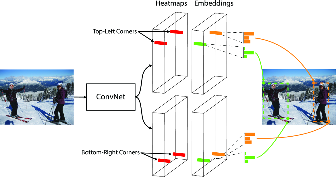
In this paper we introduce CornerNet, a new one-stage approach to object detection that does away with anchor boxes. We detect an object as a pair of keypoints—the top-left corner and bottom-right corner of the bounding box. We use a single convolutional network to predict a heatmap for the top-left corners of all instances of the same object category, a heatmap for all bottom-right corners, and an embedding vector for each detected corner. The embeddings serve to group a pair of corners that belong to the same object—the network is trained to predict similar embeddings for them. Our approach greatly simplifies the output of the network and eliminates the need for designing anchor boxes. Our approach is inspired by the associative embedding method proposed by Newell et al., (2017), who detect and group keypoints in the context of multiperson human-pose estimation. Fig. 1 illustrates the overall pipeline of our approach.

Figure 2: Often there is no local evidence to determine the location of a bounding box corner. We address this issue by proposing a new type of pooling layer.

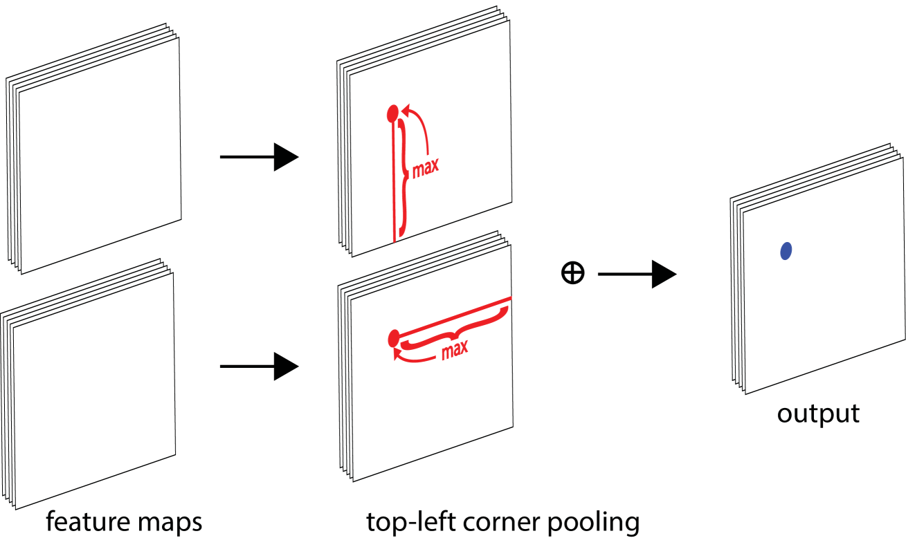
Another novel component of CornerNet is corner pooling, a new type of pooling layer that helps a convolutional network better localize corners of bounding boxes. A corner of a bounding box is often outside the object—consider the case of a circle as well as the examples in Fig. 2. In such cases a corner cannot be localized based on local evidence. Instead, to determine whether there is a top-left corner at a pixel location, we need to look horizontally towards the right for the topmost boundary of the object, and look vertically towards the bottom for the leftmost boundary. This motivates our corner pooling layer: it takes in two feature maps; at each pixel location it max-pools all feature vectors to the right from the first feature map, max-pools all feature vectors directly below from the second feature map, and then adds the two pooled results together. An example is shown in Fig. 3.

Figure 3: Corner pooling: for each channel, we take the maximum values (red dots) in two directions (red lines), each from a separate feature map, and add the two maximums together (blue dot).

We hypothesize two reasons why detecting corners would work better than bounding box centers or proposals. First, the center of a box can be harder to localize because it depends on all 4 sides of the object, whereas locating a corner depends on 2 sides and is thus easier, and even more so with corner pooling, which encodes some explicit prior knowledge about the definition of corners. Second, corners provide a more efficient way of densely discretizing the space of boxes: we just need $O(wh)$ corners to represent $O(w^{2}h^{2})$ possible anchor boxes.

We demonstrate the effectiveness of CornerNet on MS COCO (Lin et al.,, 2014). CornerNet achieves a 42.2% AP, outperforming all existing one-stage detectors. In addition, through ablation studies we show that corner pooling is critical to the superior performance of CornerNet. Code is available at https://github.com/princeton-vl/CornerNet.

2 Related Works

2.1 Two-stage object detectors

Two-stage approach was first introduced and popularized by R-CNN (Girshick et al.,, 2014). Two-stage detectors generate a sparse set of regions of interest (RoIs) and classify each of them by a network. R-CNN generates RoIs using a low level vision algorithm (Uijlings et al.,, 2013; Zitnick and Dollár,, 2014). Each region is then extracted from the image and processed by a ConvNet independently, which creates lots of redundant computations. Later, SPP (He et al.,, 2014) and Fast-RCNN (Girshick,, 2015) improve R-CNN by designing a special pooling layer that pools each region from feature maps instead. However, both still rely on separate proposal algorithms and cannot be trained end-to-end. Faster-RCNN (Ren et al.,, 2015) does away low level proposal algorithms by introducing a region proposal network (RPN), which generates proposals from a set of pre-determined candidate boxes, usually known as anchor boxes. This not only makes the detectors more efficient but also allows the detectors to be trained end-to-end. R-FCN (Dai et al.,, 2016) further improves the efficiency of Faster-RCNN by replacing the fully connected sub-detection network with a fully convolutional sub-detection network. Other works focus on incorporating sub-category information (Xiang et al.,, 2016), generating object proposals at multiple scales with more contextual information (Bell et al.,, 2016; Cai et al.,, 2016; Shrivastava et al.,, 2016; Lin et al.,, 2016), selecting better features (Zhai et al.,, 2017), improving speed (Li et al.,, 2017), cascade procedure (Cai and Vasconcelos,, 2017) and better training procedure (Singh and Davis,, 2017).

2.2 One-stage object detectors

On the other hand, YOLO (Redmon et al.,, 2016) and SSD (Liu et al.,, 2016) have popularized the one-stage approach, which removes the RoI pooling step and detects objects in a single network. One-stage detectors are usually more computationally efficient than two-stage detectors while maintaining competitive performance on different challenging benchmarks.

SSD places anchor boxes densely over feature maps from multiple scales, directly classifies and refines each anchor box. YOLO predicts bounding box coordinates directly from an image, and is later improved in YOLO9000 (Redmon and Farhadi,, 2016) by switching to anchor boxes. DSSD (Fu et al.,, 2017) and RON (Kong et al.,, 2017) adopt networks similar to the hourglass network (Newell et al.,, 2016), enabling them to combine low-level and high-level features via skip connections to predict bounding boxes more accurately. However, these one-stage detectors are still outperformed by the two-stage detectors until the introduction of RetinaNet (Lin et al.,, 2017). In (Lin et al.,, 2017), the authors suggest that the dense anchor boxes create a huge imbalance between positive and negative anchor boxes during training. This imbalance causes the training to be inefficient and hence the performance to be suboptimal. They propose a new loss, Focal Loss, to dynamically adjust the weights of each anchor box and show that their one-stage detector can outperform the two-stage detectors. RefineDet (Zhang et al.,, 2017) proposes to filter the anchor boxes to reduce the number of negative boxes, and to coarsely adjust the anchor boxes.

DeNet (Tychsen-Smith and Petersson, 2017a, ) is a two-stage detector which generates RoIs without using anchor boxes. It first determines how likely each location belongs to either the top-left, top-right, bottom-left or bottom-right corner of a bounding box. It then generates RoIs by enumerating all possible corner combinations, and follows the standard two-stage approach to classify each RoI. Our approach is very different from DeNet. First, DeNet does not identify if two corners are from the same objects and relies on a sub-detection network to reject poor RoIs. In contrast, our approach is a one-stage approach which detects and groups the corners using a single ConvNet. Second, DeNet selects features at manually determined locations relative to a region for classification, while our approach does not require any feature selection step. Third, we introduce corner pooling, a novel type of layer to enhance corner detection.

Point Linking Network (PLN) (Wang et al.,, 2017) is an one-stage detector without anchor boxes. It first predicts the locations of the four corners and the center of a bounding box. Then, at each corner location, it predicts how likely each pixel location in the image is the center. Similarly, at the center location, it predicts how likely each pixel location belongs to either the top-left, top-right, bottom-left or bottom-right corner. It combines the predictions from each corner and center pair to generate a bounding box. Finally, it merges the four bounding boxes to give a bounding box. CornerNet is very different from PLN. First, CornerNet groups the corners by predicting embedding vectors, while PLN groups the corner and center by predicting pixel locations. Second, CornerNet uses corner pooling to better localize the corners.

Our approach is inspired by Newell et al., (2017) on Associative Embedding in the context of multi-person pose estimation. Newell et al. propose an approach that detects and groups human joints in a single network. In their approach each detected human joint has an embedding vector. The joints are grouped based on the distances between their embeddings. To the best of our knowledge, we are the first to formulate the task of object detection as a task of detecting and grouping corners with embeddings. Another novelty of ours is the corner pooling layers that help better localize the corners. We also significantly modify the hourglass architecture and add our novel variant of focal loss (Lin et al.,, 2017) to help better train the network.

3 CornerNet

3.1 Overview

In CornerNet, we detect an object as a pair of keypoints—the top-left corner and bottom-right corner of the bounding box. A convolutional network predicts two sets of heatmaps to represent the locations of corners of different object categories, one set for the top-left corners and the other for the bottom-right corners. The network also predicts an embedding vector for each detected corner (Newell et al.,, 2017) such that the distance between the embeddings of two corners from the same object is small. To produce tighter bounding boxes, the network also predicts offsets to slightly adjust the locations of the corners. With the predicted heatmaps, embeddings and offsets, we apply a simple post-processing algorithm to obtain the final bounding boxes.

Figure 4: Overview of CornerNet. The backbone network is followed by two prediction modules, one for the top-left corners and the other for the bottom-right corners. Using the predictions from both modules, we locate and group the corners.

Fig. 4 provides an overview of CornerNet. We use the hourglass network (Newell et al.,, 2016) as the backbone network of CornerNet. The hourglass network is followed by two prediction modules. One module is for the top-left corners, while the other one is for the bottom-right corners. Each module has its own corner pooling module to pool features from the hourglass network before predicting the heatmaps, embeddings and offsets. Unlike many other object detectors, we do not use features from different scales to detect objects of different sizes. We only apply both modules to the output of the hourglass network.

3.2 Detecting Corners

We predict two sets of heatmaps, one for top-left corners and one for bottom-right corners. Each set of heatmaps has $C$ channels, where $C$ is the number of categories, and is of size $H\times W$. There is no background channel. Each channel is a binary mask indicating the locations of the corners for a class.

Figure 5: “Ground-truth” heatmaps for training. Boxes (green dotted rectangles) whose corners are within the radii of the positive locations (orange circles) still have large overlaps with the ground-truth annotations (red solid rectangles).

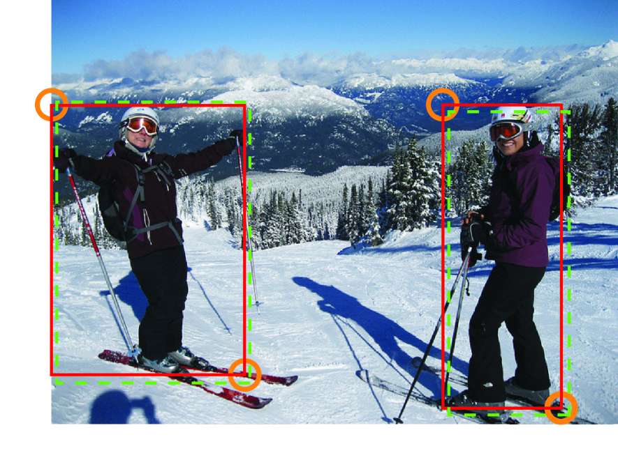
For each corner, there is one ground-truth positive location, and all other locations are negative. During training, instead of equally penalizing negative locations, we reduce the penalty given to negative locations within a radius of the positive location. This is because a pair of false corner detections, if they are close to their respective ground truth locations, can still produce a box that sufficiently overlaps the ground-truth box (Fig. 5). We determine the radius by the size of an object by ensuring that a pair of points within the radius would generate a bounding box with at least $t$ IoU with the ground-truth annotation (we set $t$ to $0.3$ in all experiments). Given the radius, the amount of penalty reduction is given by an unnormalized 2D Gaussian, $e^{-\frac{x^{2}+y^{2}}{2\sigma^{2}}}$, whose center is at the positive location and whose $\sigma$ is 1/3 of the radius.

Let $p_{cij}$ be the score at location $(i,j)$ for class $c$ in the predicted heatmaps, and let $y_{cij}$ be the “ground-truth” heatmap augmented with the unnormalized Gaussians. We design a variant of focal loss (Lin et al.,, 2017):

where $N$ is the number of objects in an image, and $\alpha$ and $\beta$ are the hyper-parameters which control the contribution of each point (we set $\alpha$ to 2 and $\beta$ to 4 in all experiments). With the Gaussian bumps encoded in $y_{cij}$, the $(1-y_{cij})$ term reduces the penalty around the ground truth locations.

Many networks (He et al.,, 2016; Newell et al.,, 2016) involve downsampling layers to gather global information and to reduce memory usage. When they are applied to an image fully convolutionally, the size of the output is usually smaller than the image. Hence, a location $(x,y)$ in the image is mapped to the location $\left(\lfloor\frac{x}{n}\rfloor,\lfloor\frac{y}{n}\rfloor\right)$ in the heatmaps, where $n$ is the downsampling factor. When we remap the locations from the heatmaps to the input image, some precision may be lost, which can greatly affect the IoU of small bounding boxes with their ground truths. To address this issue we predict location offsets to slightly adjust the corner locations before remapping them to the input resolution.

$$\bm{o}_{k}=\left(\frac{x_{k}}{n}-\left\lfloor\frac{x_{k}}{n}\right\rfloor,\frac{y_{k}}{n}-\left\lfloor\frac{y_{k}}{n}\right\rfloor\right)$$ (2)

where $\bm{o}_{k}$ is the offset, $x_{k}$ and $y_{k}$ are the x and y coordinate for corner $k$. In particular, we predict one set of offsets shared by the top-left corners of all categories, and another set shared by the bottom-right corners. For training, we apply the smooth L1 Loss (Girshick,, 2015) at ground-truth corner locations:

$$L_{\mathit{off}}=\frac{1}{N}\sum^{N}_{k=1}\text{SmoothL1Loss}\left(\bm{o}_{k},\bm{\hat{o}}_{k}\right)$$ (3)

3.3 Grouping Corners

Multiple objects may appear in an image, and thus multiple top-left and bottom-right corners may be detected. We need to determine if a pair of the top-left corner and bottom-right corner is from the same bounding box. Our approach is inspired by the Associative Embedding method proposed by Newell et al., (2017) for the task of multi-person pose estimation. Newell et al. detect all human joints and generate an embedding for each detected joint. They group the joints based on the distances between the embeddings.

The idea of associative embedding is also applicable to our task. The network predicts an embedding vector for each detected corner such that if a top-left corner and a bottom-right corner belong to the same bounding box, the distance between their embeddings should be small. We can then group the corners based on the distances between the embeddings of the top-left and bottom-right corners. The actual values of the embeddings are unimportant. Only the distances between the embeddings are used to group the corners.

We follow Newell et al., (2017) and use embeddings of 1 dimension. Let $e_{t_{k}}$ be the embedding for the top-left corner of object $k$ and $e_{b_{k}}$ for the bottom-right corner. As in Newell and Deng, (2017), we use the “pull” loss to train the network to group the corners and the “push” loss to separate the corners:

$$L_{pull}=\frac{1}{N}\sum^{N}_{k=1}\left[\left(e_{t_{k}}-e_{k}\right)^{2}+\left(e_{b_{k}}-e_{k}\right)^{2}\right],$$ (4)

$$L_{push}=\frac{1}{N(N-1)}\sum^{N}_{k=1}\sum^{N}\limits_{\begin{subarray}{c}j=1\\ j\neq k\end{subarray}}\max\left(0,\Delta-\left|e_{k}-e_{j}\right|\right),$$ (5)

where $e_{k}$ is the average of $e_{t_{k}}$ and $e_{b_{k}}$ and we set $\Delta$ to be $1$ in all our experiments. Similar to the offset loss, we only apply the losses at the ground-truth corner location.

3.4 Corner Pooling

As shown in Fig. 2, there is often no local visual evidence for the presence of corners. To determine if a pixel is a top-left corner, we need to look horizontally towards the right for the topmost boundary of an object and vertically towards the bottom for the leftmost boundary. We thus propose corner pooling to better localize the corners by encoding explicit prior knowledge.

Figure 6: The top-left corner pooling layer can be implemented very efficiently. We scan from right to left for the horizontal max-pooling and from bottom to top for the vertical max-pooling. We then add two max-pooled feature maps.

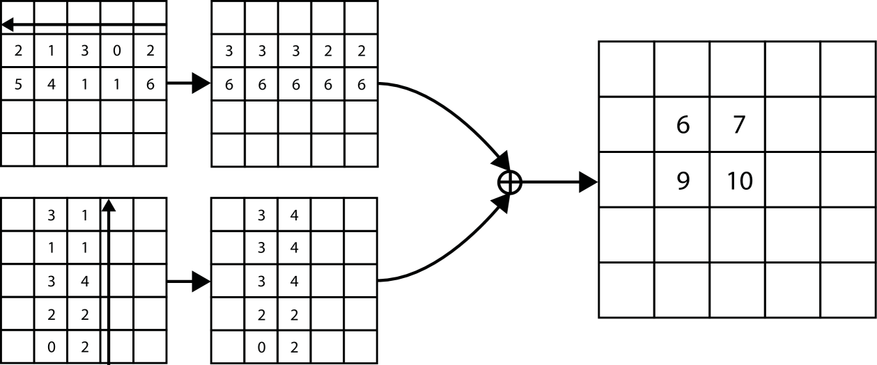
Suppose we want to determine if a pixel at location $(i,j)$ is a top-left corner. Let $f_{t}$ and $f_{l}$ be the feature maps that are the inputs to the top-left corner pooling layer, and let $f_{t_{ij}}$ and $f_{l_{ij}}$ be the vectors at location $(i,j)$ in $f_{t}$ and $f_{l}$ respectively. With $H\times W$ feature maps, the corner pooling layer first max-pools all feature vectors between $(i,j)$ and $(i,H)$ in $f_{t}$ to a feature vector $t_{ij}$, and max-pools all feature vectors between $(i,j)$ and $(W,j)$ in $f_{l}$ to a feature vector $l_{ij}$. Finally, it adds $t_{ij}$ and $l_{ij}$ together. This computation can be expressed by the following equations:

$$t_{ij}=\left\{\begin{matrix}\max\left(f_{t_{ij}},t_{(i+1)j}\right)&\text{if}\ i<H\\ f_{t_{Hj}}&\text{otherwise}\end{matrix}\right.$$ (6)

$$l_{ij}=\left\{\begin{matrix}\max\left(f_{l_{ij}},l_{i(j+1)}\right)&\text{if}\ j<W\\ f_{l_{iW}}&\text{otherwise}\end{matrix}\right.$$ (7)

where we apply an elementwise $\max$ operation. Both $t_{ij}$ and $l_{ij}$ can be computed efficiently by dynamic programming as shown Fig. 8.

We define bottom-right corner pooling layer in a similar way. It max-pools all feature vectors between $(0,j)$ and $(i,j)$, and all feature vectors between $(i,0)$ and $(i,j)$ before adding the pooled results. The corner pooling layers are used in the prediction modules to predict heatmaps, embeddings and offsets.

Figure 7: The prediction module starts with a modified residual block, in which we replace the first convolution module with our corner pooling module. The modified residual block is then followed by a convolution module. We have multiple branches for predicting the heatmaps, embeddings and offsets.

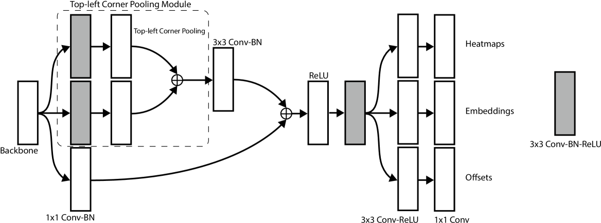
The architecture of the prediction module is shown in Fig. 7. The first part of the module is a modified version of the residual block (He et al.,, 2016). In this modified residual block, we replace the first $3\times 3$ convolution module with a corner pooling module, which first processes the features from the backbone network by two $3\times 3$ convolution modules  with 128 channels and then applies a corner pooling layer. Following the design of a residual block, we then feed the pooled features into a $3\times 3$ Conv-BN layer with 256 channels and add back the projection shortcut. The modified residual block is followed by a $3\times 3$ convolution module with 256 channels, and 3 Conv-ReLU-Conv layers to produce the heatmaps, embeddings and offsets.

3.5 Hourglass Network

CornerNet uses the hourglass network (Newell et al.,, 2016) as its backbone network. The hourglass network was first introduced for the human pose estimation task. It is a fully convolutional neural network that consists of one or more hourglass modules. An hourglass module first downsamples the input features by a series of convolution and max pooling layers. It then upsamples the features back to the original resolution by a series of upsampling and convolution layers. Since details are lost in the max pooling layers, skip layers are added to bring back the details to the upsampled features. The hourglass module captures both global and local features in a single unified structure. When multiple hourglass modules are stacked in the network, the hourglass modules can reprocess the features to capture higher-level of information. These properties make the hourglass network an ideal choice for object detection as well. In fact, many current detectors (Shrivastava et al.,, 2016; Fu et al.,, 2017; Lin et al.,, 2016; Kong et al.,, 2017) already adopted networks similar to the hourglass network.

Our hourglass network consists of two hourglasses, and we make some modifications to the architecture of the hourglass module. Instead of using max pooling, we simply use stride 2 to reduce feature resolution. We reduce feature resolutions 5 times and increase the number of feature channels along the way ($256,384,384,384,512$). When we upsample the features, we apply 2 residual modules followed by a nearest neighbor upsampling. Every skip connection also consists of 2 residual modules. There are 4 residual modules with 512 channels in the middle of an hourglass module. Before the hourglass modules, we reduce the image resolution by 4 times using a $7\times 7$ convolution module with stride 2 and 128 channels followed by a residual block (He et al.,, 2016) with stride 2 and 256 channels.

Following (Newell et al.,, 2016), we also add intermediate supervision in training. However, we do not add back the intermediate predictions to the network as we find that this hurts the performance of the network. We apply a $1\times 1$ Conv-BN module to both the input and output of the first hourglass module. We then merge them by element-wise addition followed by a ReLU and a residual block with 256 channels, which is then used as the input to the second hourglass module. The depth of the hourglass network is 104. Unlike many other state-of-the-art detectors, we only use the features from the last layer of the whole network to make predictions.

Table 1: Ablation on corner pooling on MS COCO validation.

	AP	$\text{AP}^{50}$	$\text{AP}^{75}$	$\text{AP}^{s}$	$\text{AP}^{m}$	$\text{AP}^{l}$
w/o corner pooling	36.5	52.0	38.8	17.5	38.9	49.4
w/ corner pooling	38.4	53.8	40.9	18.6	40.5	51.8
improvement	+2.0	+2.1	+2.1	+1.1	+2.4	+3.6

Table 2: Reducing the penalty given to the negative locations near positive locations helps significantly improve the performance of the network

	AP	$\text{AP}^{50}$	$\text{AP}^{75}$	$\text{AP}^{s}$	$\text{AP}^{m}$	$\text{AP}^{l}$
w/o reducing penalty	32.9	49.1	34.8	19.0	37.0	40.7
fixed radius	35.6	52.5	37.7	18.7	38.5	46.0
object-dependent radius	38.4	53.8	40.9	18.6	40.5	51.8

Table 3: Corner pooling consistently improves the network performance on detecting corners in different image quadrants, showing that corner pooling is effective and stable over both small and large areas.

	mAP w/o pooling	mAP w/ pooling	improvement
Top-Left Corners
Top-Left Quad.	66.1	69.2	+3.1
Bottom-Right Quad.	60.8	63.5	+2.7
Bottom-Right Corners
Top-Left Quad.	53.4	56.2	+2.8
Bottom-Right Quad.	65.0	67.6	+2.6

4 Experiments

4.1 Training Details

We implement CornerNet in PyTorch (Paszke et al.,, 2017). The network is randomly initialized under the default setting of PyTorch with no pretraining on any external dataset. As we apply focal loss, we follow (Lin et al.,, 2017) to set the biases in the convolution layers that predict the corner heatmaps. During training, we set the input resolution of the network to $511\times 511$, which leads to an output resolution of $128\times 128$. To reduce overfitting, we adopt standard data augmentation techniques including random horizontal flipping, random scaling, random cropping and random color jittering, which includes adjusting the brightness, saturation and contrast of an image. Finally, we apply PCA (Krizhevsky et al.,, 2012) to the input image.

We use Adam (Kingma and Ba,, 2014) to optimize the full training loss:

$$L=L_{det}+\alpha L_{pull}+\beta L_{push}+\gamma L_{\mathit{off}}$$ (8)

where $\alpha$, $\beta$ and $\gamma$ are the weights for the pull, push and offset loss respectively. We set both $\alpha$ and $\beta$ to 0.1 and $\gamma$ to 1. We find that 1 or larger values of $\alpha$ and $\beta$ lead to poor performance. We use a batch size of 49 and train the network on 10 Titan X (PASCAL) GPUs (4 images on the master GPU, 5 images per GPU for the rest of the GPUs). To conserve GPU resources, in our ablation experiments, we train the networks for 250k iterations with a learning rate of $2.5\times 10^{-4}$. When we compare our results with other detectors, we train the networks for an extra 250k iterations and reduce the learning rate to $2.5\times 10^{-5}$ for the last 50k iterations.

Figure 8: Qualitative examples showing corner pooling helps better localize the corners.

4.2 Testing Details

During testing, we use a simple post-processing algorithm to generate bounding boxes from the heatmaps, embeddings and offsets. We first apply non-maximal suppression (NMS) by using a $3\times 3$ max pooling layer on the corner heatmaps. Then we pick the top 100 top-left and top 100 bottom-right corners from the heatmaps. The corner locations are adjusted by the corresponding offsets. We calculate the L1 distances between the embeddings of the top-left and bottom-right corners. Pairs that have distances greater than 0.5 or contain corners from different categories are rejected. The average scores of the top-left and bottom-right corners are used as the detection scores.

Instead of resizing an image to a fixed size, we maintain the original resolution of the image and pad it with zeros before feeding it to CornerNet. Both the original and flipped images are used for testing. We combine the detections from the original and flipped images, and apply soft-nms (Bodla et al.,, 2017) to suppress redundant detections. Only the top 100 detections are reported. The average inference time is 244ms per image on a Titan X (PASCAL) GPU.

4.3 MS COCO

We evaluate CornerNet on the very challenging MS COCO dataset (Lin et al.,, 2014). MS COCO contains 80k images for training, 40k for validation and 20k for testing. All images in the training set and 35k images in the validation set are used for training. The remaining 5k images in validation set are used for hyper-parameter searching and ablation study. All results on the test set are submitted to an external server for evaluation. To provide fair comparisons with other detectors, we report our main results on the test-dev set. MS COCO uses average precisions (APs) at different IoUs and APs for different object sizes as the main evaluation metrics.

Table 4: The hourglass network is crucial to the performance of CornerNet.

	AP	$\text{AP}^{50}$	$\text{AP}^{75}$	$\text{AP}^{s}$	$\text{AP}^{m}$	$\text{AP}^{l}$
FPN (w/ ResNet-101) + Corners	30.2	44.1	32.0	13.3	33.3	42.7
Hourglass + Anchors	32.9	53.1	35.6	16.5	38.5	45.0
Hourglass + Corners	38.4	53.8	40.9	18.6	40.5	51.8

4.4 Ablation Study

4.4.1 Corner Pooling

Corner pooling is a key component of CornerNet. To understand its contribution to performance, we train another network without corner pooling but with the same number of parameters.

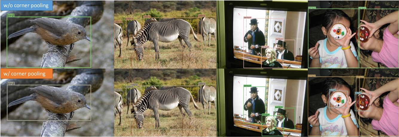
Tab. 1 shows that adding corner pooling gives significant improvement: 2.0% on AP, 2.1% on $\text{AP}^{50}$ and 2.1% on $\text{AP}^{75}$. We also see that corner pooling is especially helpful for medium and large objects, improving their APs by 2.4% and 3.6% respectively. This is expected because the topmost, bottommost, leftmost, rightmost boundaries of medium and large objects are likely to be further away from the corner locations. Fig. 8 shows four qualitative examples with and without corner pooling.

Table 5: CornerNet performs much better at high IoUs than other state-of-the-art detectors.

	AP	$\text{AP}^{50}$	$\text{AP}^{60}$	$\text{AP}^{70}$	$\text{AP}^{80}$	$\text{AP}^{90}$
RetinaNet (Lin et al.,, 2017)	39.8	59.5	55.6	48.2	36.4	15.1
Cascade R-CNN (Cai and Vasconcelos,, 2017)	38.9	57.8	53.4	46.9	35.8	15.8
Cascade R-CNN + IoU Net (Jiang et al.,, 2018)	41.4	59.3	55.3	49.6	39.4	19.5
CornerNet	40.6	56.1	52.0	46.8	38.8	23.4

Table 6: Error analysis. We replace the predicted heatmaps and offsets with the ground-truth values. Using the ground-truth heatmaps alone improves the AP from 38.4% to 73.1%, suggesting that the main bottleneck of CornerNet is detecting corners.

	AP	$\text{AP}^{50}$	$\text{AP}^{75}$	$\text{AP}^{s}$	$\text{AP}^{m}$	$\text{AP}^{l}$
	38.4	53.8	40.9	18.6	40.5	51.8
w/ gt heatmaps	73.1	87.7	78.4	60.9	81.2	81.8
w/ gt heatmaps + offsets	86.1	88.9	85.5	84.8	87.2	82.0

Figure 9: Qualitative example showing errors in predicting corners and embeddings. The first row shows images where CornerNet mistakenly combines boundary evidence from different objects. The second row shows images where CornerNet predicts similar embeddings for corners from different objects.

Table 7: CornerNet versus others on MS COCO test-dev. CornerNet outperforms all one-stage detectors and achieves results competitive to two-stage detectors

Method	Backbone	AP	$\text{AP}^{50}$	$\text{AP}^{75}$	$\text{AP}^{s}$	$\text{AP}^{m}$	$\text{AP}^{l}$	$\text{AR}^{1}$	$\text{AR}^{10}$	$\text{AR}^{100}$	$\text{AR}^{s}$	$\text{AR}^{m}$	$\text{AR}^{l}$
Two-stage detectors
DeNet (Tychsen-Smith and Petersson, 2017a, )	ResNet-101	33.8	53.4	36.1	12.3	36.1	50.8	29.6	42.6	43.5	19.2	46.9	64.3
CoupleNet (Zhu et al.,, 2017)	ResNet-101	34.4	54.8	37.2	13.4	38.1	50.8	30.0	45.0	46.4	20.7	53.1	68.5
Faster R-CNN by G-RMI (Huang et al.,, 2017)	Inception-ResNet-v2 (Szegedy et al.,, 2017)	34.7	55.5	36.7	13.5	38.1	52.0	-	-	-	-	-	-
Faster R-CNN+++ (He et al.,, 2016)	ResNet-101	34.9	55.7	37.4	15.6	38.7	50.9	-	-	-	-	-	-
Faster R-CNN w/ FPN (Lin et al.,, 2016)	ResNet-101	36.2	59.1	39.0	18.2	39.0	48.2	-	-	-	-	-	-
Faster R-CNN w/ TDM (Shrivastava et al.,, 2016)	Inception-ResNet-v2	36.8	57.7	39.2	16.2	39.8	52.1	31.6	49.3	51.9	28.1	56.6	71.1
D-FCN (Dai et al.,, 2017)	Aligned-Inception-ResNet	37.5	58.0	-	19.4	40.1	52.5	-	-	-	-	-	-
Regionlets (Xu et al.,, 2017)	ResNet-101	39.3	59.8	-	21.7	43.7	50.9	-	-	-	-	-	-
Mask R-CNN (He et al.,, 2017)	ResNeXt-101	39.8	62.3	43.4	22.1	43.2	51.2	-	-	-	-	-	-
Soft-NMS (Bodla et al.,, 2017)	Aligned-Inception-ResNet	40.9	62.8	-	23.3	43.6	53.3	-	-	-	-	-	-
LH R-CNN (Li et al.,, 2017)	ResNet-101	41.5	-	-	25.2	45.3	53.1	-	-	-	-	-	-
Fitness-NMS (Tychsen-Smith and Petersson, 2017b, )	ResNet-101	41.8	60.9	44.9	21.5	45.0	57.5	-	-	-	-	-	-
Cascade R-CNN (Cai and Vasconcelos,, 2017)	ResNet-101	42.8	62.1	46.3	23.7	45.5	55.2	-	-	-	-	-	-
D-RFCN + SNIP (Singh and Davis,, 2017)	DPN-98 (Chen et al.,, 2017)	45.7	67.3	51.1	29.3	48.8	57.1	-	-	-	-	-	-
One-stage detectors
YOLOv2 (Redmon and Farhadi,, 2016)	DarkNet-19	21.6	44.0	19.2	5.0	22.4	35.5	20.7	31.6	33.3	9.8	36.5	54.4
DSOD300 (Shen et al., 2017a, )	DS/64-192-48-1	29.3	47.3	30.6	9.4	31.5	47.0	27.3	40.7	43.0	16.7	47.1	65.0
GRP-DSOD320 (Shen et al., 2017b, )	DS/64-192-48-1	30.0	47.9	31.8	10.9	33.6	46.3	28.0	42.1	44.5	18.8	49.1	65.0
SSD513 (Liu et al.,, 2016)	ResNet-101	31.2	50.4	33.3	10.2	34.5	49.8	28.3	42.1	44.4	17.6	49.2	65.8
DSSD513 (Fu et al.,, 2017)	ResNet-101	33.2	53.3	35.2	13.0	35.4	51.1	28.9	43.5	46.2	21.8	49.1	66.4
RefineDet512 (single scale) (Zhang et al.,, 2017)	ResNet-101	36.4	57.5	39.5	16.6	39.9	51.4	-	-	-	-	-	-
RetinaNet800 (Lin et al.,, 2017)	ResNet-101	39.1	59.1	42.3	21.8	42.7	50.2	-	-	-	-	-	-
RefineDet512 (multi scale) (Zhang et al.,, 2017)	ResNet-101	41.8	62.9	45.7	25.6	45.1	54.1	-	-	-	-	-	-
CornerNet511 (single scale)	Hourglass-104	40.6	56.4	43.2	19.1	42.8	54.3	35.3	54.7	59.4	37.4	62.4	77.2
CornerNet511 (multi scale)	Hourglass-104	42.2	57.8	45.2	20.7	44.8	56.6	36.6	55.9	60.3	39.5	63.2	77.3

4.4.2 Stability of Corner Pooling over Larger Area

Corner pooling pools over different sizes of area in different quadrants of an image. For example, the top-left corner pooling pools over larger areas both horizontally and vertically in the upper-left quadrant of an image, compared to the lower-right quadrant. Therefore, the location of a corner may affect the stability of the corner pooling.

We evaluate the performance of our network on detecting both the top-left and bottom-right corners in different quadrants of an image. Detecting corners can be seen as a binary classification task i.e. the ground-truth location of a corner is positive, and any location outside of a small radius of the corner is negative. We measure the performance using mAPs over all categories on the MS COCO validation set.

Tab. 3 shows that without corner pooling, the top-left corner mAPs of upper-left and lower-right quadrant are $66.1\%$ and $60.8\%$ respectively. Top-left corner pooling improves the mAPs by $3.1\%$ (to $69.2\%$) and $2.7\%$ (to $63.5\%$) respectively. Similarly, bottom-right corner pooling improves the bottom-right corner mAPs of upper-left quadrant by $2.8\%$ (from $53.4\%$ to $56.2\%$), and lower-right quadrant by $2.6\%$ (from $65.0\%$ to $67.6\%$). Corner pooling gives similar improvement to corners at different quadrants, show that corner pooling is effective and stable over both small and large areas.

4.4.3 Reducing Penalty to Negative Locations

We reduce the penalty given to negative locations around a positive location, within a radius determined by the size of the object (Sec. 3.2). To understand how this helps train CornerNet, we train one network with no penalty reduction and another network with a fixed radius of $2.5$. We compare them with CornerNet on the validation set.

Tab. 2 shows that a fixed radius improves AP over the baseline by 2.7%, $\text{AP}^{m}$ by 1.5% and $\text{AP}^{l}$ by 5.3%. Object-dependent radius further improves the AP by 2.8%, $\text{AP}^{m}$ by 2.0% and $\text{AP}^{l}$ by 5.8%. In addition, we see that the penalty reduction especially benefits medium and large objects.

4.4.4 Hourglass Network

CornerNet uses the hourglass network (Newell et al.,, 2016) as its backbone network. Since the hourglass network is not commonly used in other state-of-the-art detectors, we perform an experiment to study the contribution of the hourglass network in CornerNet. We train a CornerNet in which we replace the hourglass network with FPN (w/ ResNet-101) (Lin et al.,, 2017), which is more commonly used in state-of-the-art object detectors. We only use the final output of FPN for predictions. Meanwhile, we train an anchor box based detector which uses the hourglass network as its backbone. Each hourglass module predicts anchor boxes at multiple resolutions by using features at multiple scales during upsampling stage. We follow the anchor box design in RetinaNet (Lin et al.,, 2017) and add intermediate supervisions during training. In both experiments, we initialize the networks from scratch and follow the same training procedure as we train CornerNet (Sec. 4.1).

Tab. 4 shows that CornerNet with hourglass network outperforms CornerNet with FPN by $8.2\%$ AP, and the anchor box based detector with hourglass network by $5.5\%$ AP. The results suggest that the choice of the backbone network is important and the hourglass network is crucial to the performance of CornerNet.

Figure 10: Example bounding box predictions overlaid on predicted heatmaps of corners.

4.4.5 Quality of the Bounding Boxes

A good detector should predict high quality bounding boxes that cover objects tightly. To understand the quality of the bounding boxes predicted by CornerNet, we evaluate the performance of CornerNet at multiple IoU thresholds, and compare the results with other state-of-the-art detectors, including RetinaNet (Lin et al.,, 2017), Cascade R-CNN (Cai and Vasconcelos,, 2017) and IoU-Net (Jiang et al.,, 2018).

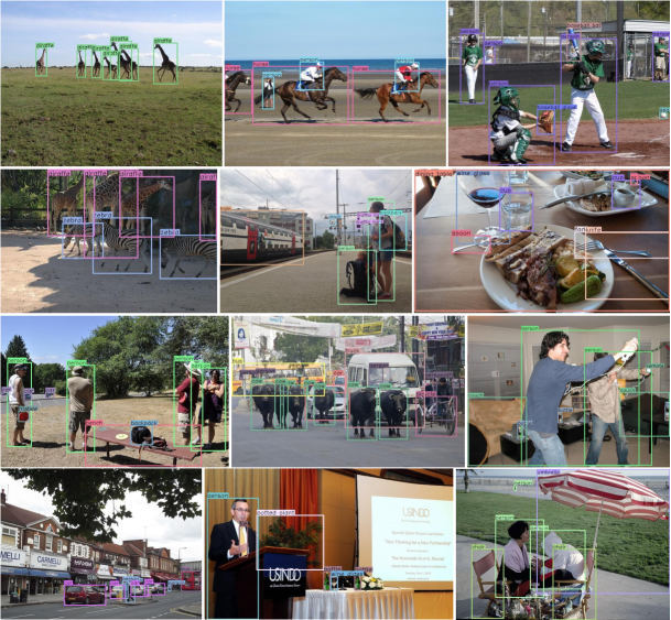
Tab. 5 shows that CornerNet achieves a much higher AP at 0.9 IoU than other detectors, outperforming Cascade R-CNN + IoU-Net by $3.9\%$, Cascade R-CNN by $7.6\%$ and RetinaNet  by $7.3\%$. This suggests that CornerNet is able to generate bounding boxes of higher quality compared to other state-of-the-art detectors.

Figure 11: Qualitative examples on MS COCO.

4.4.6 Error Analysis

CornerNet simultaneously outputs heatmaps, offsets, and embeddings, all of which affect detection performance. An object will be missed if either corner is missed; precise offsets are needed to generate tight bounding boxes; incorrect embeddings will result in many false bounding boxes. To understand how each part contributes to the final error, we perform an error analysis by replacing the predicted heatmaps and offsets with the ground-truth values and evaluting performance on the validation set.

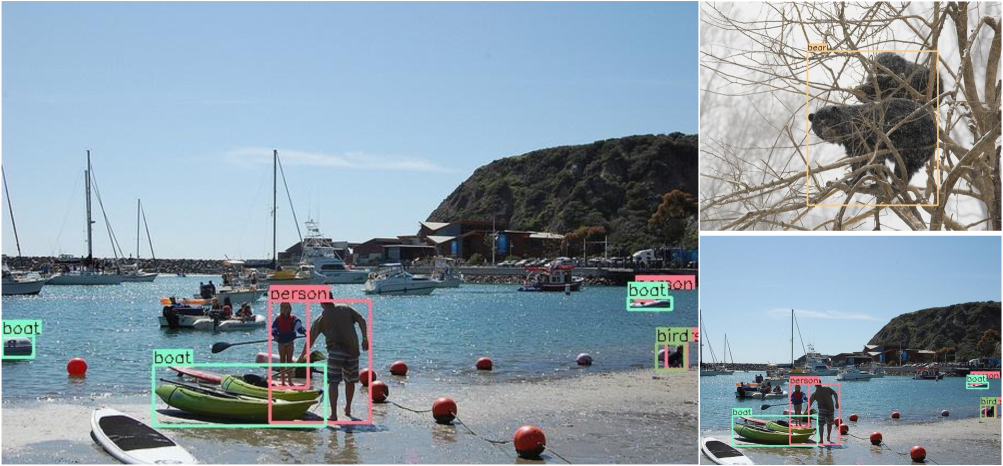
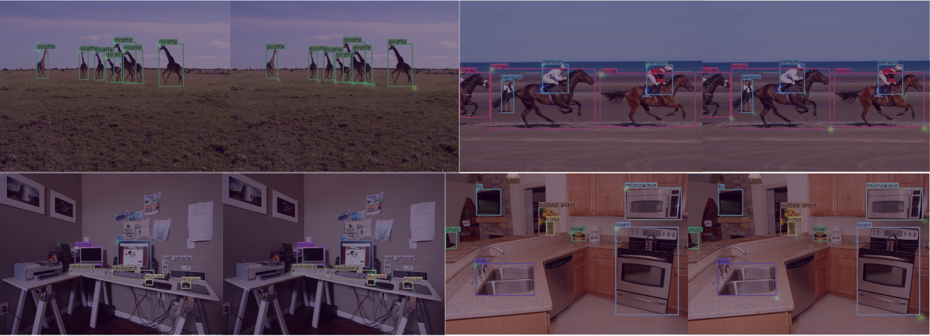
Tab. 6 shows that using the ground-truth corner heatmaps alone improves the AP from 38.4% to 73.1%. $\text{AP}^{s}$, $\text{AP}^{m}$ and $\text{AP}^{l}$ also increase by 42.3%, 40.7% and 30.0% respectively. If we replace the predicted offsets with the ground-truth offsets, the AP further increases by 13.0% to 86.1%. This suggests that although there is still ample room for improvement in both detecting and grouping corners, the main bottleneck is detecting corners. Fig. 9 shows some qualitative examples where the corner locations or embeddings are incorrect.

4.5 Comparisons with state-of-the-art detectors

We compare CornerNet with other state-of-the-art detectors on MS COCO test-dev (Tab. 7). With multi-scale evaluation, CornerNet achieves an AP of 42.2%, the state of the art among existing one-stage methods and competitive with two-stage methods.

5 Conclusion

We have presented CornerNet, a new approach to object detection that detects bounding boxes as pairs of corners. We evaluate CornerNet on MS COCO and demonstrate competitive results.