Structured Neural Network Dynamics
for Model-based Control

Abstract

We present a structured neural network architecture that is inspired by linear time-varying dynamical systems. The network is designed to mimic the properties of linear dynamical systems which makes analysis and control simple. The architecture facilitates the integration of learned system models with gradient-based model predictive control algorithms, and removes the requirement of computing potentially costly derivatives online. We demonstrate the efficacy of this modeling technique in computing autonomous control policies through evaluation in a variety of standard continuous control domains.

I Introduction and Background

The question of how to best generate autonomous control policies for mechanical systems is an important problem in robotics. Research in this field can be traced back to early work on optimal control by Pontryagin [20] and Bellman [5]. Since this time, significant progress has been made in both the theory and application of autonomous control techniques [22, 24]. However, challenges remain in developing strategies that are valid without a priori knowledge of the system dynamics.

One possible solution is to use model-free policy generation techniques [9]. These methods require no explicit model of the system dynamics and have been shown to be effective in numerous domains [14, 15]. However, model-free policy generation techniques often require massive amounts of data and are therefore difficult to evaluate on real-world robotic systems [9]. An alternative option is to learn an explicit model of the system dynamics which can be incorporated into an optimal control algorithm. Model-based control methods are more data-efficient and often easier to apply in real-world scenarios [3, 6]. However, many optimal control algorithms require some notion of derivatives to compute a control policy [2, 16, 18, 25].

Figure 1: Structured neural network architecture for model-based predictive control. The final layer of the $A$-subnet must be the same dimension as the state space, and the final layer of the $B$-subnet must be the same dimension as the control space. The network then computes a function of the form $\dot{x}=A\cdot x+B\cdot u$. This structure makes it easy to recover time-varying derivatives (i.e., $A,B$) for use in model predictive control algorithms.

Computing the required derivatives can often prove challenging with complex modeling techniques like deep neural networks [4]. Additionally, these black-box methods make it difficult to analyze the underlying dynamics of the system. There are, of course, alternative modeling techniques [1, 3, 8, 11, 13, 15]; however, there remains a desire to incorporate modern, deep neural networks into the optimization loop due to their ability to model challenging dynamic features (e.g., contacts) and scale to high-dimensional tasks [12, 19, 27]. In this work, we provide a method that combines the expressive power of neural network models with gradient-based optimal control algorithms. Our solution is based on a neural network architecture that enforces a linear structure in the state and control space, making it easier to analyze and incorporate into model-based control.

II Structured Neural Networks for
Model Predictive Control

In this section, we define our structured neural network architecture and then detail how the learned models can be integrated into model-based control algorithms.

II-A Structured Neural Network Architecture

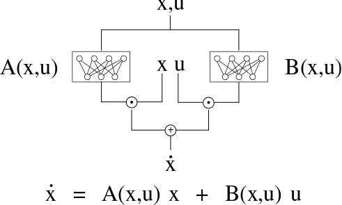
Our neural network architecture is composed of two parallel subnetworks (see Figure 1). The architecture of the first subnetwork ($A$-subnet) can be defined by any number of layers and parameters, and is only constrained such that the final layer must have $N$ parameters, where $N$ is the dimension of the system’s state space. Similarly, the second subnetwork ($B$-subnet) is only constrained such that the final layer must have $M$ parameters, where $M$ is the dimension of the system’s control space. The network then combines (1) the dot product of the output from the $A$-subnet and the state $x$, with (2) the dot product of the output from the $B$-subnet and the control $u$, through an element-wise add operation. This architecture describes a single, global model of the form $\dot{x}=A(x,u)\cdot x+B(x,u)\cdot u$, which is trained with standard gradient-based techniques and can be evaluated and linearized anywhere in the state space. Here, the $A$-subnet represents the linearization of the dynamics model with respect to the state variables (i.e., $\frac{\partial f}{\partial x}$), and the $B$-subnet represents the linearization of the dynamics model with respect to the control variables (i.e., $\frac{\partial f}{\partial u}$).

II-B Integration with Model-based Control

Given a learned dynamics model, one can compute autonomous control policies through data-driven methods [12] or through integration with optimal control algorithms [2, 16, 25]. On the optimal control side, researchers have mostly explored sampling-based optimization methods. For example, researchers have proposed computing control trajectories with a random shooting method [19] and with model predictive path integral [27] control. The reason that sampling-based methods are appealing in this domain is that the solution does not depend on computing potentially costly gradients with respect to the state and control variables. However, the solution does require generating a large number of samples to cover a sufficient portion of the action space. The challenge, then, is to balance the number of samples generated at each time-step with the rate of the control loop. As the dimensionality of the action space grows, this becomes more and more challenging.

In contrast with sampling-based methods, gradient-based optimization techniques provide an efficient method of computing control trajectories. Additionally, these methods provide sensitivity information in the form of time-varying Jacobians. However, integrating neural network models with these optimization techniques can prove difficult. This is because it is unclear a priori how to compute the necessary Jacobians ($\frac{\partial f}{\partial x}$, and $\frac{\partial f}{\partial u}$). By enforcing a linear structure on the neural network architecture (as described in Section II-A), we can efficiently predict the evolution of the dynamic system as well as the required Jacobians. Then, to generate an autonomous policy, we solve the following optimal control problem

$$\underset{u}{\text{minimize}} J=\int_{t=0}^{T-1}l(x(t),u(t))+l_{T}(x(T))$$ (1)

subject to $$\dot{x}(t)=f_{\theta}(x(t),u(t)),$$

$$u(t)\in U,x(t)\in X,\forall t$$

where $f_{\theta}(x(t),u(t))$ is the learned, structured system dynamics, $l$ and $l_{T}$ are the running and terminal cost, and $U$ and $X$ are the set of valid control and state values. The solution of this problem is the control sequence that minimizes the cost.

(a) Mountain Car

(b) Cart-Pole

(c) Two-Link Arm

(d) Mountain Car

(e) Cart Pole

(f) Two Link Arm

Figure 2: Subfigures (a), (b), and (c) are pictorial representations of our experimental environments. Subfigures (d), (e), and (f) are state diagrams demonstrating the efficacy of our model-based control algorithm.

III Experimental Validation

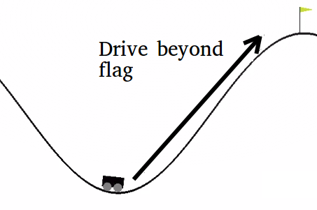
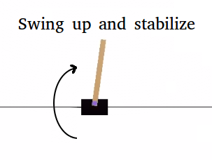
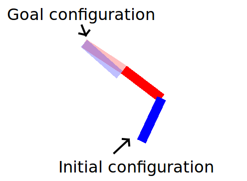
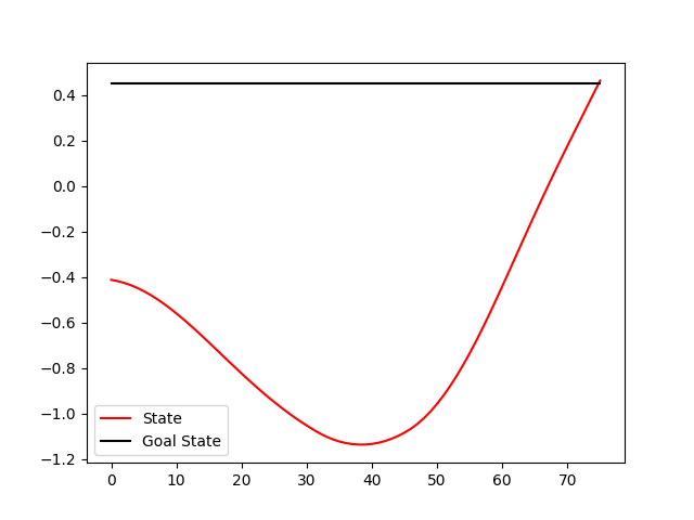
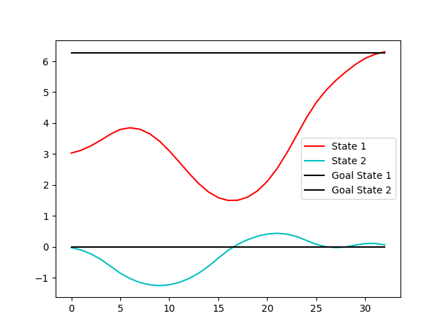
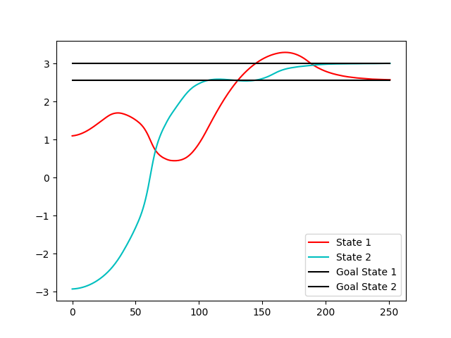
We validate the efficacy of our described approach through experimentation on three standard control domains. Our first experimental environment is OpenAI’s implementation of the continuous mountain car problem [7] (Figure 2(a)). The mountain car is defined by a two dimensional state space ($x,\dot{x}$) and one dimensional control space ($\ddot{x}$). The second experimental environment is an implementation of the classic cart-pole swing up problem written from scratch (Figure 2(b)). The cart-pole is defined by a four dimensional state space ($x,\dot{x},\theta,\dot{\theta}$) and a one dimensional control space ($\ddot{x}$). The final experimental environment is a two-link arm written in the Bullet physics engine and described in a related CMU course (Figure 2(c)). The two-link arm exists in a four dimensional state space ($\theta_{1},\dot{\theta_{1}},\theta_{2},\dot{\theta_{2}}$) and is controlled with a two dimensional signal ($\ddot{\theta_{1}},\ddot{\theta_{2}}$). All three environments are defined with continuous-valued state and control spaces.

III-A Model Learning Details

In this section, we describe our data collection method and the training procedure.

III-A1 Data collection

We collect data through observation of trajectories produced by the system using control inputs sampled uniformly at random. The data is collected in tuples of ($x(t),u(t),\dot{x(t)}$), where $\dot{x}(t)$ is computed as $\frac{x(t)-x(t-1)}{dt}$ and $dt$ is the timestep. For each environment, we collect 500 trajectories, which are terminated at either 500 steps or when the system violates environment boundary or safety conditions.

III-A2 Training the model

Given a dataset of tuples ($x(t),u(t),\dot{x(t)}$), we train the dynamics model $f_{\theta}(x(t),u(t))$ by minimizing the following error function

$${\varepsilon}=\sum_{(x(t),u(t),\dot{x}(t))\in D}\frac{1}{2}||f_{\theta}(x(t),u(t))-\dot{x}(t)||^{2}$$ (2)

We use the Adam optimizer with a learning rate of 0.001. Half the data is used for training and half for validation. We find that no data preprocessing is necessary.

IV Results

Our evaluation consists of state plots which demonstrate that our defined neural network architecture can be used to solve model-based control problems. Each example solution depicts the initial state of the system (the start of the state trajectory, which is chosen at random), the time-varying state produced by our model-based control algorithm (red and blue), and the goal state (black). In Figures 2(d), 2(e), 2(f), we relay a single solution for each experimental environment, however, we note that our algorithm produced successful control trajectories (with respect to the desired goal state) from a variety of initial conditions. Additionally, our approach was able to successfully generate control trajectories that reached arbitrary goal states in the two-link arm environment.

These results suggest that our structured neural network can be used to learn a global model of the system dynamics, while simultaneously enforcing linearization constraints that make it possible to recover time-varying derivatives without additional computation. In contrast to approximation methods (e.g., numerical differentiation) and symbolic methods (e.g., automatic differentiation), our approach can be thought of as a prediction method for computing the required time-varying derivatives. Related work in this area includes the transformation network proposed in [26] which directly predicts the parameters of an A and B matrix in a latent space. In contrast, our approach does not explicitly learn parameters of a matrix; instead we learn nonlinear mappings (A-subnet, B-subnet) that we treat as linearizations of the global model in the structure of our network network. This allows us to learn a global model of the system dynamics, while simultaneously enforcing linearization constraints. A related call for the use of structure in neural networks has been explored in model-free policy generation. In [23], researchers describe a network architecture that combines linear and nonlinear policies into a single control model. In our work, we instead enforce structure that mimics linear time-varying systems, and incorporate these models into optimal control algorithms.

IV-A Why We Think This Works

In this work, we address the bottleneck associated with computing gradients of the system model through the application of a structured neural network that explicitly encodes linearization constraints and therefore reduces the computational complexity necessary to recover the required Jacobians. However, without further study, it is not clear whether or not the learned $A$ and $B$-subnetworks actually approximate the required time-varying derivatives. Experimental evidence suggests that the vectors represented by these networks are, at a minimum, pointing in the direction of the gradient. This claim is based on the fact that (1) our model-based control algorithm produces successful policies in a variety of control domains, and (2) when we incorporate the learned system model into an MPC algorithm, we treat the output of the subnetworks as first order derivatives of the system dynamics.

IV-B Open Questions

We now pose a number of open questions that we plan to address in future work. In particular, we are interested in exploring how our structured neural network model compares with alternative methods of computing time-varying derivatives. One such solution is to use a finite differences method for numerical differentiation. From a practical standpoint, we note that this method is prone to round-off errors and is computationally expensive in an iterative, receding-horizon framework. Another solution is to use automatic differentiation [4]. This approach has been shown to work well, however it requires well formed expression graphs and derivatives computed at compile-time to work efficiently enough for online optimization [10]. In future work, we plan to compare and contrast these methods in high-dimensional control spaces.

V Conclusion

In this work, we propose a structured neural network that can be used to solve model-based control problems. The architecture makes it easy to integrate the learned models with gradient-based optimal control algorithms and simplifies the interpretation of a system model parameterized by a deep neural network. This idea is inline with other recent calls for simplification of data-driven control strategies such as [17, 21].

References

- Abraham et al. [2017] Ian Abraham, Gerardo De La Torre, and Todd Murphey. Model-Based Control Using Koopman Operators. In Robotics: Science and Systems, 2017.
- Ansari and Murphey [2016] Alex Ansari and Todd D Murphey. Sequential Action Control: Closed-Form Optimal Control for Nonlinear Systems. IEEE Transactions on Robotics, 32:1196 – 1214, Oct. 2016.
- Atkeson and Santamaria [1997] Christopher G Atkeson and Juan Carlos Santamaria. A Comparison of Direct and Model-based Reinforcement Learning. In International Conference on Robotics and Automation, volume 4, pages 3557–3564. IEEE, 1997.
- Baydin et al. [2018] Atilim Gunes Baydin, Barak A Pearlmutter, Alexey Andreyevich Radul, and Jeffrey Mark Siskind. Automatic Differentiation in Machine Learning: A Survey. Journal of Machine Learning Research, 18(153):1–43, 2018.
- Bellman [1957] Richard Bellman. Dynamic Programming. Princeton University Press, 1957.
- Broad et al. [2017] Alexander Broad, Todd Murphey, and Brenna Argall. Learning Models for Shared Control of Human-Machine Systems with Unknown Dynamics. In Robotics: Science and Systems, 2017.
- Brockman et al. [2016] Greg Brockman, Vicki Cheung, Ludwig Pettersson, Jonas Schneider, John Schulman, Jie Tang, and Wojciech Zaremba. OpenAI Gym. arXiv:1606.01540, 2016.
- Deisenroth and Rasmussen [2011] Marc Deisenroth and Carl E Rasmussen. PILCO: A Model-Based and Data-Efficient Approach to Policy Search. In International Conference on Machine Learning, pages 465–472, 2011.
- Deisenroth et al. [2013] Marc Peter Deisenroth, Gerhard Neumann, Jan Peters, et al. A Survey on Policy Search for Robotics. Foundations and Trends in Robotics, 2(1–2):1–142, 2013.
- Giftthaler et al. [2017] Markus Giftthaler, Michael Neunert, Markus Stäuble, Marco Frigerio, Claudio Semini, and Jonas Buchli. Automatic Differentiation of Rigid Body Dynamics for Optimal Control and Estimation. Advanced Robotics, 31(22):1225–1237, 2017.
- Gu et al. [2016] Shixiang Gu, Timothy Lillicrap, Ilya Sutskever, and Sergey Levine. Continuous Deep Q-Learning with Model-based Acceleration. In International Conference on Machine Learning, pages 2829–2838, 2016.
- Heess et al. [2015] Nicolas Heess, Gregory Wayne, David Silver, Tim Lillicrap, Tom Erez, and Yuval Tassa. Learning Continuous Control Policies by Stochastic Value Gradients. In Advances in Neural Information Processing Systems, pages 2944–2952, 2015.
- Khansari-Zadeh and Billard [2011] S Mohammad Khansari-Zadeh and Aude Billard. Learning Stable Nonlinear Dynamical Systems with Gaussian Mixture Models. IEEE Transactions on Robotics, 27(5):943–957, 2011.
- Kober and Peters [2009] Jens Kober and Jan R Peters. Policy Search for Motor Primitives in Robotics. In Advances in Neural Information Processing Systems, pages 849–856, 2009.
- Levine and Abbeel [2014] Sergey Levine and Pieter Abbeel. Learning Neural Network Policies with Guided Policy Search Under Unknown Dynamics. In Advances in Neural Information Processing Systems, pages 1071–1079, 2014.
- [16] Weiwei Li and Emanuel Todorov. Iterative Linear Quadratic Regulator Design for Nonlinear Biological Movement Systems. In International Conference on Informatics in Control, Automation and Robotics, pages 222–229.
- Mania et al. [2018] Horia Mania, Aurelia Guy, and Benjamin Recht. Simple Sandom Search Provides a Competitive Approach to Reinforcement Learning. arXiv:1803.07055, 2018.
- Mayne [1973] David Q Mayne. Differential Dynamic Programming–A Unified Approach to the Optimization of Dynamic Systems. In Control and Dynamic Systems, volume 10, pages 179–254. Elsevier, 1973.
- Nagabandi et al. [2017] Anusha Nagabandi, Gregory Kahn, Ronald S Fearing, and Sergey Levine. Neural Network Dynamics for Model-based Deep Reinforcement Learning with Model-free Fine-Tuning. arXiv:1708.02596, 2017.
- Pontryagin [1987] Lev Semenovich Pontryagin. The Mathematical Theory of Optimal Processes. CRC Press, 1987.
- Rajeswaran et al. [2017] Aravind Rajeswaran, Kendall Lowrey, Emanuel V Todorov, and Sham M Kakade. Towards Generalization and Simplicity in Continuous Control. In Advances in Neural Information Processing Systems, pages 6553–6564, 2017.
- Sontag [2013] Eduardo D Sontag. Mathematical Control Theory: Deterministic Finite Dimensional Systems, volume 6. Springer Science & Business Media, 2013.
- Srouji et al. [2018] Mario Srouji, Jian Zhang, and Ruslan Salakhutdinov. Structured Control Nets for Deep Reinforcement Learning. International Conference on Machine Learning, 2018.
- Sutton and Barto [2017] Richard S Sutton and Andrew G Barto. Reinforcement Learning: An Introduction, volume 2. MIT press Cambridge, 2017.
- Tassa et al. [2014] Yuval Tassa, Nicolas Mansard, and Emo Todorov. Control-Limited Differential Dynamic Programming. In International Conference on Robotics and Automation, pages 1168–1175. IEEE, 2014.
- Watter et al. [2015] Manuel Watter, Jost Springenberg, Joschka Boedecker, and Martin Riedmiller. Embed to Control: A Locally Linear Latent Dynamics Model for Control from Raw Images. In Advances in Neural Information Processing Systems, pages 2746–2754, 2015.
- Williams et al. [2017] Grady Williams, Nolan Wagener, Brian Goldfain, Paul Drews, James M Rehg, Byron Boots, and Evangelos A Theodorou. Information Theoretic MPC for Model-based Reinforcement Learning. In International Conference on Robotics and Automation, pages 1714–1721. IEEE, 2017.