Stretched Exponential Relaxation

1 The stretched exponential

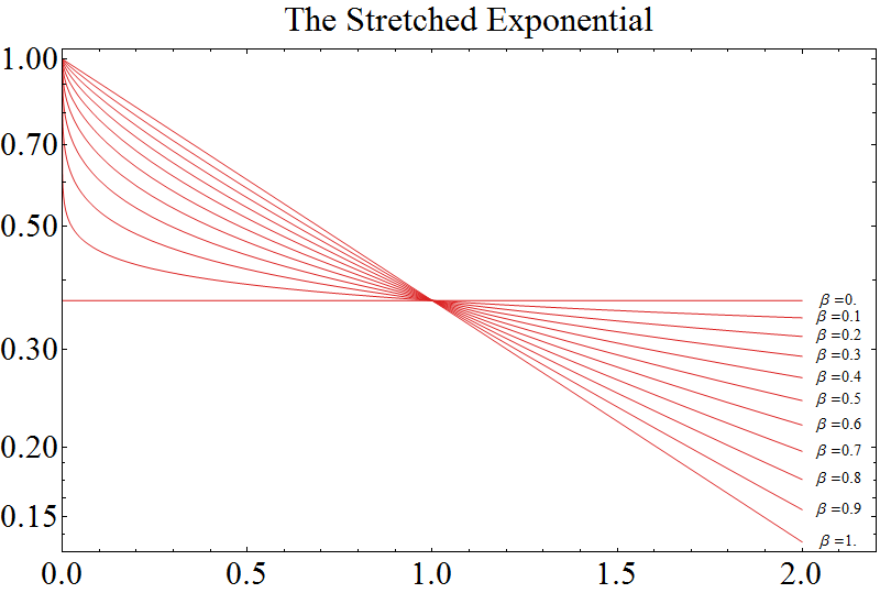
Figure 1: The stretched exponential on a log plot for various values of $\beta$

The stretched exponential is:

$$\phi(t)=A\exp\left[-\left(\frac{t}{\tau_{\mbox{\footnotesize{str}}}}\right)^{\beta}\right]$$ (1)

Rudolf (Hermann Arndt) Kohlrausch ( 1809 - 1858) first proposed the stretched exponential in 1854 to describe the relaxation of charge from a glass Leiden jar.[11]

He came to expression 1 by assuming that the decay rate $k=1/tau$ was not constant but deceased with time as $t^{\beta-1}$.

The stretched exponential has an exceptionally wide range of application throughout science. In the materials science and engineering literature, an expression known as the “Weibull distribution” is used , with $\beta$ taking any value. (For $\beta=2$ the Gaussian distribution is obtained) In the social/economic sciences it is used to describe things such as urban population sizes, currency exchange rate fluctuations, and the success of Hollywood blockbusters, musicians and scientists. (Since it has a fat tail, like the power law it is useful in describing “rich get richer” phenomena which are widespread in the social sciences). In 1993 Bömer listed stretching exponents for over 70 materials, obtained by viscoelastic, calorimetric, dielectric, optical, and other response measurements.

In mathematics, the stretched exponential is the characteristic function (Fourier transform of) a type of stable distribution called the (Lévy) “symmetric alpha-stable distribution”. (There is no general analytic expression for the Fourier transform of the stretched exponential, so this class of distributions is defined simply as the Fourier transform of the stretched exponential - this point is discussed further below).

In the field of dielectric spectroscopy it is often refereed to as the Williams-Watts (WW) or Kohlrausch-Williams-Watts (KWW) function after a paper by Williams & Watts in 1970.[18]

In all of its many applications, the stretched exponential distribution never gives the entire picture, but as a phenomenological function it can often describe data over many orders of magnitude. The fact that it contains only one extra parameter, $\beta$, makes it exceptionally easy to fit to data, but as we will see it does not have clean mathematical properties like the Gaussian or exponential function, both of which are special cases of the stretched exponential. The fact that such a simple analytic expression can fit data over many orders of magnitudes suggests, but by no means proves, that it must be of some fundamental significance. In the field of glasses though, it can be said with good confidence that the stretched exponential has some truly fundamental significance. Even the simplest theoretical model of a glass - the 3D $\pm J$ spin glass on a cubic lattice - exhibits stretched exponential relaxation in the spin-spin autocorrelation function, as has now been conclusively shown by computer simulation. A nearly linear decrease in $\beta(T)$ as a function of temperature is observed - decreasing from $\beta=1$ at the Curie point $\approx 4.5T_{g}$ to $\beta=.35$ at the glass transition temperature $T_{g}$.

In the studies of relaxation of glasses, theoretical justification can be found in the so-called “trapping model”, which was first developed in the 1970s by mathematical physicists to describe the non-radiative recombination of excitons in amorphous semiconductors. The mathematical intricacies of the trapping model are quite complex, but the basic idea is rather simple to visualize. It is assumed that the material is filled with randomly distributed traps. Traps capture excitations whenever they are within a certain radius of the trap. During relaxation, excitons (or more generally, molecules) diffuse through the material and fill these traps. As the traps are filled, the remaining excitons must travel for longer to find unfilled traps, thus explaining the $k=t^{\beta-1}$ decrease in the rate. In particular, the trapping model predicts:

$$\beta=\frac{d}{d+2}$$ (2)

In three dimensions, the trapping model gives $\beta=3/5=.6$. There have been many other attempts to give the stretched exponential a theoretical justification, mostly in the field of glasses and disordered materials – a review of these theories and the related experimental data was given by J.C. Phillips in 1996, with the focus mainly on the trapping model.[15] According to Phillips the trapping model is the only model which describes the emergence of the stretched exponential in truly microscopic terms and does so with mathematical rigor (albeit only with great effort, requiring concepts from axiomatic set theory).[15] Furthermore, Phillips argues that the trapping model is much more widely applicable than was previously thought.

Klafter identifies three separate models which yield a stretched exponential relaxation – the Förster energy transfer model, the hierarchically constrained dynamics picture and the “defect diffusion model” – and he shows that all three share mathematical similarities.[8]

Models yielding stretched exponential relaxation can be divided into two types - serial and parallel.[3] (Additionally, there are references in the literature suggesting that it might necessary to combine both). In a serial model, relaxation proceeds through a number of steps separated by barriers of different heights. In a parallel model, each molecule is relaxing exponentially through a single barrier, but there are different barrier heights for different molecules.

The author of this article has studied dielectic relaxation in water with molecular dynamics simulation, noting how the rotational relaxation of molecules follows a stretched exponential form.[4] Possible serial and parallel explanations for this were explored.[4] Counter intuitvely, the overall dielectric relaxation of water is largely exponential,[5] but interestly the dielectric relaxation becomes stretched exponential in nano-confined water.[16]

1.1 Mathematical properties of the stretched exponential

1.1.1 $\tau$ distribution

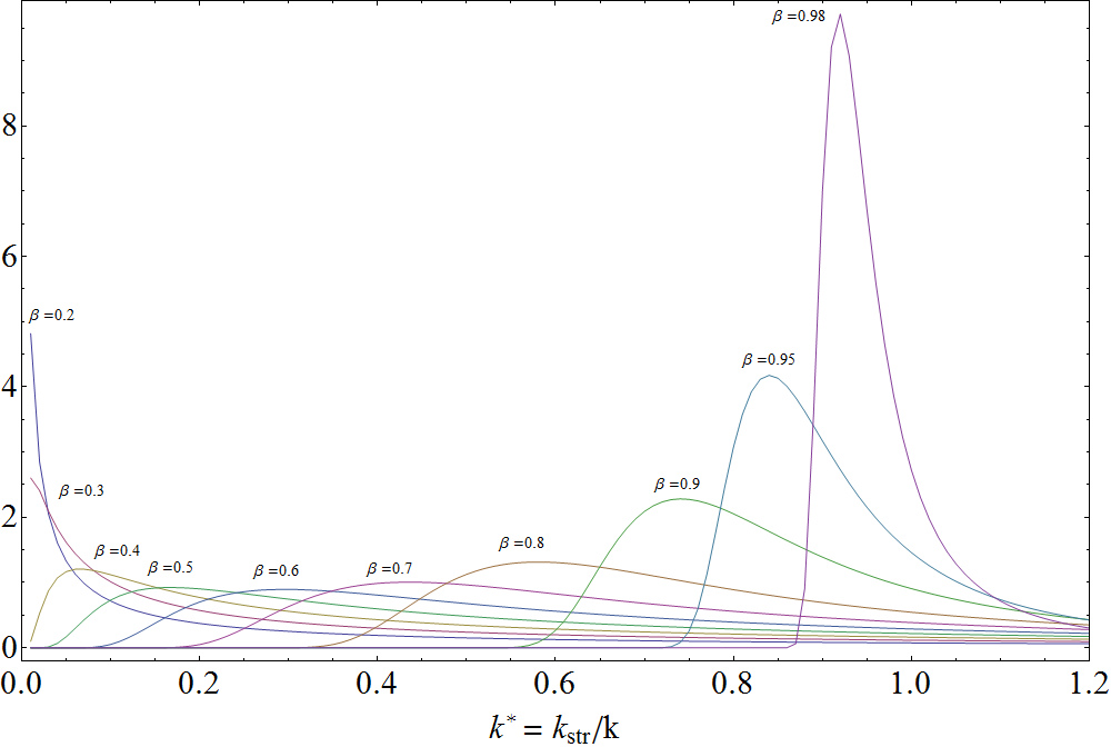
Figure 2: $G(k)$ distribution for various values of $\beta$.

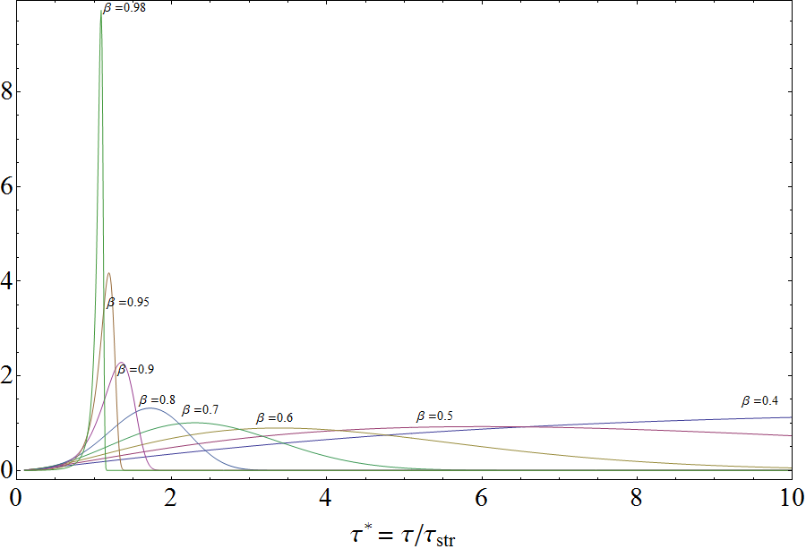
Figure 3: Same data as in fig. 2 but showing $G(\tau)$ for various values of $\beta$. (It appears that the normalization was lost during the transformation)

The stretched exponential can be understood as a continuous sum of exponential decays via the following transformation:

$$\exp\left[-\left(\frac{t}{\tau_{\mbox{\footnotesize{str}}}}\right)^{\beta}\right]=\int_{0}^{\infty}P(s,\beta)\exp(-s\frac{t}{\tau_{\mbox{\tiny{str}}}})ds$$ (3)

Here $s$ is defined as the dimensionless variable $s\equiv k/k_{\mbox{\footnotesize{str}}}=\tau_{\mbox{\footnotesize{str}}}/\tau$.

Equation 3 is an example of a Laplace transform, thus, to recover $P(s,\beta)$ requires taking the inverse Laplace transform:

$$P(s,\beta)=\frac{1}{2\pi i}\int_{\Gamma}e^{-x^{\beta}}e^{sx}dx$$ (4)

Where $\Gamma$ is a path from $-i\infty$ to $i\infty$ such that all the singularities in the integrand lie on the left.

A change of variables $u=ix$ allows one to write this as a Fourier transform:

$$P(s,\beta)=\frac{1}{2\pi}\int_{-\infty}^{\infty}e^{-(iu)^{\beta}}e^{isu}du$$ (5)

$P(s,\beta)$ is a probability distribution normalized to one. Mathematically, these distributions are asymmetric Lévy stable distributions.[7] (Not to be confused with the symmetric Lévy stable distributions, of which the stretched exponential is the characteristic function). (More precisely stated, there is a one-to-one correspondance between the asymmetric Lévy stable distributions and the space of functions of the form $\exp((kt)^{\beta})$ where $\beta\in(0,2)$.) Just as the centralized limit says that idd random variables sampled from distributions with finite variance will eventually converge to a Gaussian, the generalized centralized central limit theorem says that iid variables taken from distributions with power law tails of the form $|x|^{-\beta-1}$ ($\beta\in(0,2)$) will lead to Asymmetric Lévy stable distributions (since power law tails are not normalizable, a special normalization factor $1/N^{1/\beta}$ must be used to construct the limiting distribution).[12] In light of this fact the ubiquitous nature of the stretched exponential is not as surprising, since power law distributions are also ubiquitous.

A few different formulae have been derived for calculating $P(s,\beta)$ for arbitrary $\beta$. One is a summation formula:

$$P(s,\beta)=\frac{1}{\pi}\sum_{n=1}^{\infty}\frac{(-1)^{n+1}\Gamma(n\beta+1)}{n!s^{n\beta+1}}\sin(n\pi\beta)$$ (6)

The convergence of this series appears to be very slow – to produce good plots $\approx$ 10,000 terms were required, thus making use of this formula very cumbersome even on a fast machine. A better equation can be obtained by looking at the real and imaginary parts of equation 5. It can be shown that the imaginary part is exactly zero (which is good because imaginary probabilities don’t make much sense). The real part is:[6]

$$P(s,\beta)=\frac{1}{\pi}\int_{0}^{\infty}e^{-u^{\beta}\cos(\pi\beta/2)}\cos[su-u^{\beta}\sin(\pi\beta/2)]du$$ (7)

A rigorous derivation of this formula is given in [13] using different notation. Equation 7 evaluates much faster in Mathematica (production of a nice looking plot of $P(s,\beta)$ at $\approx$ 1000 points takes about 1.5 minutes distributed over four 2.2 GHz i7 cores).

It is also possible to obtain so-called “closed form expressions” (in terms of Airy, Bessel, Gamma, hypergeometric and complex error functions) from for rational values of $\beta=n/m$, although these expressions rapidly increase in complexity as with larger $m$. A particularly nice closed form expression is obtained for $\beta=1/2$:

$$P(s,\frac{1}{2})=\frac{1}{\sqrt{4\pi s^{3}}}\exp\left(-\frac{1}{4s}\right)$$ (8)

The case $\beta=1/2$ was studied exclusively by Williams & Watts in their seminal paper.

1.1.2 Behavior near zero

Near zero the stretched exponential exhibits a singularity in its derivative. In fact, this singularity appears at all higher orders of derivatives as well. When $t\ll\tau_{\mbox{\footnotesize{str}}}$ one finds

$$s\phi(t)\approx A-A\beta\left(\frac{t}{\tau_{\mbox{\footnotesize{str}}}}\right)^{\beta}$$ (9)

1.2 Properties of $G(k)/G(\tau)$

The properties and limiting behavior of $P(s,\beta)$ are studied in detail by Johnson in his work to better understand how to interpret both $\beta$ and $k_{\mbox{\footnotesize{str}}}$.[6] We will not go through his detailed analysis here, but will note some of the key results because they are very illuminating.

• The max in $G(\tau)$ increases with increasing $\beta$ in a way which can be fit by an exponential function

• $G(k)$ contains a low-$k$ (high $\tau$) exponential cutoff that decreases with decreasing $\beta$.

• $G(k)$ contains a power law tail at high k described by :

  $$P(k\rightarrow\infty) =\frac{c}{s^{1+\beta}}$$ (10)

  $$c =\frac{\Gamma(\beta+1)}{\pi}\sin(\pi\beta)$$

• The first moment (average) of $G(k)$ is infinite

• All higher moments of $G(k)$ are infinite

• The moments of $G(\tau)$ are finite and are given by:

  $$\langle\tau^{m}\rangle=\frac{\Gamma(m/\beta)}{\beta\Gamma(m)}$$ (11)

• $k_{\mbox{\footnotesize{str}}}$ in the stretched exponential function is not the average rate, nor is it the inverse of the average $\tau$. It is approximately the median $k$, but only for $.5\beta 1$.

• The $\beta$ factor cannot in any way be used to describe adequately the “width” of the distribution $G(k)$. However it is related monotonically to the low $k$ (large $\tau$) cutoff. From the average of $G(\tau)$ another interpretation is that $1/\beta$ is a measure of the average relaxation time relative to $\tau_{\mbox{\footnotesize{str}}}$.

1.3 Barrier height distributions

For a system where the higher energy state is separated from the lower energy state by a barrier of height $E_{a}$, the relaxation time (assuming Arrhenius behavior) is related to $E_{a}$ via:

$$k =k_{0}e^{-\frac{E}{kT}}=\tau_{0}e^{-\epsilon}$$ (12)

$$E =-kT\ln(k/k_{0})=-kT\ln(\tau_{0}/\tau)$$

This allow one to transform $P(s,\beta)$ into $P(E_{a},\beta)$, which is a distribution of barrier heights. A way of calculating these barrier height distributions and approximating them by analytic functions was discussed by Edholm & Blomberg in 2000.[3] These distributions look like skewed Gaussians, with skewness towards the smaller energies. In the limit of $\beta\rightarrow 0$ the distribution becomes Gaussian, but the approach is not a smooth approach - even for values of $\beta$ close to zero the distribution remains very skewed. Edholm & Blomberg note that the approximate width of the barrier height distribution is well described by

$$\sigma=1/\beta$$ (13)

for $0<\beta<.85$. They also note that for $0<\beta<.85$ the distribution can be somewhat approximated by a Gaussian and analyze how good this approximation is. One one might therefore wonder what happens if we just assume a Gaussian barrier height distribution. Unfortunately this leads to taking the inverse Laplace transform of an expression of the form $\exp(\exp(x^{2}))$, for which no closed form expression is known.

References

- [1] M. Berberan-Santos, E.N. Bodunov, and B. Valeur. History of the kohlrausch (stretched exponential) function: Pioneering work in luminescence. Annalen der Physik, 17(7):460–461, 2008.
- [2] M. Cardona, R.V. Chamberlin, and W. Marx. The history of the stretched exponential function. Annalen der Physik, 16(12):842–845, 2007.
- [3] Olle Edholm and Clas Blomberg. Stretched exponentials and barrier distributions. Chemical Physics, 252(1–2):221 – 225, 2000.
- [4] Daniel C. Elton. PhD Thesis : “Understanding the Dielectric Properties of Water”. PhD thesis, Stony Brook University, 2016.
- [5] Daniel C. Elton. The origin of the debye relaxation in liquid water and fitting the high frequency excess response. Phys. Chem. Chem. Phys., 19:18739–18749, 2017.
- [6] D. C. Johnston. Stretched exponential relaxation arising from a continuous sum of exponential decays. Phys. Rev. B, 74:184430, Nov 2006.
- [7] A. Jurlewicz and K. Weron. A relationship between asymmetric lévy-stable distributions and the dielectric susceptibility. Journal of Statistical Physics, 73:69–81, 1993.
- [8] Joseph Klafter and Michael F. Shlesinger. On the relationship among three theories of relaxation in disordered systems. Proceedings of the National Academy of Sciences, 83(4):848–851, 1986.
- [9] F. Kohlrausch. Ueber die elastische nachwirkung bei der torsion. Annalen der Physik, 195(7):337–368, 1863.
- [10] R. Kohlrausch. Pogg. Ann. Phys. Chem., 72:353–393, 1847.
- [11] R. Kohlrausch. Theorie des elektrischen rückstandes in der leidener flasche. Annalen der Physik, 167(2):179–214, 1854.
- [12] Ismo Koponen. Random transition rate model of stretched exponential relaxation. Journal of Non-Crystalline Solids, 189(1–2):154 – 160, 1995.
- [13] Larry S. Liebovitch and Tibor I. Tóth. Distributions of activation energy barriers that produce stretched exponential probability distributions for the time spent in each state of the two state reaction a⇌b. Bulletin of Mathematical Biology, 53:443–455, 1991.
- [14] M. Mézard, G. Parisi, and M.Á. Virasoro. Spin Glass Theory and Beyond. World Scientific Lecture Notes in Physics. World Scientific, 1987.
- [15] J. C. Phillips. Stretched exponential relaxation in molecular and electronic glasses. Reports on Progress in Physics, 59(9):1133, 1996.
- [16] Adarsh Shekhar, Rajiv K. Kalia, Aiichiro Nakano, Priya Vashishta, Camilla K. Alm, and Anders Malthe-Sørenssen. Universal stretched exponential relaxation in nanoconfined water. Applied Physics Letters, 105(16):161907, 2014.
- [17] A. Werner. Quantitatie messungen der an- und abklingung getrennter phosphorescenzbanden. Annalen der Physik, 24:64, 1907.
- [18] Graham Williams and David C. Watts. Non-symmetrical dielectric relaxation behaviour arising from a simple empirical decay function. Trans. Faraday Soc., 66:80–85, 1970.