Isothermal Bondi accretion in two-component Jaffe galaxies with a central black hole

Abstract

The fully analytical solution for isothermal Bondi accretion on a black hole (MBH) at the center of two-component Jaffe (1983) galaxy models is presented. In a previous work we provided the analytical expressions for the critical accretion parameter and the radial profile of the Mach number in the case of accretion on a MBH at the center of a spherically symmetric one-component Jaffe galaxy model. Here we apply this solution to galaxy models where both the stellar and total mass density distributions are described by the Jaffe profile, with different scale-lengths and masses, and to which a central MBH is added. For such galaxy models all the relevant stellar dynamical properties can also be derived analytically (Ciotti & Ziaee Lorzad 2018). In these new models the hydrodynamical and stellar dynamical properties are linked by imposing that the gas temperature is proportional to the virial temperature of the galaxy stellar component. The formulae that are provided allow to evaluate all flow properties, and are then useful for estimates of the scale-radius and the mass flow rate when modeling accretion on massive black holes at the center of galaxies. As an application, we quantify the departure from the true mass accretion rate of estimates obtained using the gas properties at various distances from the MBH, under the hypothesis of classical Bondi accretion.

1. Introduction

Observational and numerical investigations of accretion on massive black holes (hereafter MBH) at the center of galaxies often lack the resolution to follow gas transport down to the parsec scale. In these cases, the classical Bondi (1952) solution for spherically-symmetric, steady accretion of a spatially infinite gas distribution onto a central point mass is then commonly adopted; this is the standard reference for estimates of the accretion radius (i.e., the sonic radius), and the mass accretion rate (see, e.g., Rafferty et al. 2006, Sijacki et al. 2007; Di Matteo et al. 2008; Gallo et al. 2010; Pellegrini 2010; Barai et al. 2011; Bu et al. 2013; Cao 2016; Volonteri et al. 2015; Choi et al. 2017; Park et al. 2017; Beckmann et al. 2018; Ramírez-Velasquez et al. 2018; Barai et al. 2018). Even though highly idealized, during phases of moderate accretion (in the “maintainance” mode), indeed, the problem can be considered almost steady, and Bondi accretion could provide a reliable approximation of the real situation (e.g., Barai et al. 2012, Ciotti & Ostriker 2012).

However, leaving aside the validity of the fundamental assumptions of spherical symmetry, stationarity, and optical thinness, two major problems affect the direct application of the classical Bondi solution, namely the facts that 1) the boundary values of density and temperature of the accreting gas should be evaluated at infinity, and 2) in a galaxy, the gas experiences the gravitational effects of the galaxy itself (stars plus dark matter) all the way down to the central MBH, and the MBH gravity becomes dominant only in the very central regions, inside the so-called “sphere-of-influence”. The solution commonly adopted in numerical and observational applications to alleviate these problems is to use values of the gas density and temperature “sufficiently near” the MBH, thus assuming that the galaxy effects are negligible. Of course, as the density and temperature of the accreting gas change along the pathlines, also the predictions of classical Bondi accretion will change, when based on the density and temperature measured at a finite distance from the MBH. It is therefore of great interest to be able to quantify the systematic effects on the accretion radius and the mass accretion rate obtained from the classical Bondi solution, due to measurements taken at finite distance from the MBH, and under the effects of the galaxy potential well.

A first step towards a quantititative analysis of this problem was carried out in Korol et al. (2016, hereafter KCP16) where the Bondi problem was generalized to the case of mass accretion at the center of galaxies, including also the effect of electron scattering on the accreting gas. KCP16 then calculated the deviation from the true values of the estimates of the Bondi radius and of the mass accretion rate, due to adopting as boundary values for the density and temperature those at a finite distance from the MBH, and assuming the validity of the classical Bondi accretion solution. In the specific case of Hernquist (1990) galaxies, KCP16 obtained the analytical expression of the critical accretion parameter, as a function of the galaxy properties and of the gas polytropic index $\gamma$. However, even for this quite exceptional case, the radial profiles of the hydrodynamical variables remained to be determined numerically. Following KCP16, Ciotti & Pellegrini (2017, hereafter CP17) showed that the whole accretion solution can be given in an analytical way (in terms of the Lambert-Euler $W$-function) for the isothermal accretion in Jaffe (1983) and Hernquist galaxy models with central MBHs. This meant that for these models not only it is possible to express analytically the critical accretion parameter, but also that the whole radial profile of the Mach number (and then of all the hydrodynamical functions) can be explicitely written. At the best of our knowledge, CP17 provided the first fully analytical solution of the accretion problem on a MBH at the center of a galaxy.

The galaxy models used in KCP16 and CP17, i.e., the Hernquist and Jaffe models, are not only relevant because for them it is possible to solve the accretion problem, but also because of their numerous applications in Stellar Dynamics. In fact, these models belong to the family of the so-called $\gamma$-models (Dehnen 1993, Tremaine et al. 1994) and are known to reproduce very well the radial trend of the stellar density distribution of real elliptical galaxies; at the same time, their simplicity allows for analytical studies of one and two-component galaxy models (e.g., Carollo et al. 1995, Ciotti et al. 1996, Ciotti 1999). In particular, Ciotti & Ziaee Lorzad (2018, hereafter CZ18), expanding a previous study by Ciotti et al. (2009), presented spherically symmetric two-component galaxy models (hereafter JJ models), where the stellar and total mass density distributions are both described by the Jaffe profile, with different scale-lengths and masses, and a MBH is added at the center. The orbital structure of the stellar component is described by the Osipkov-Merritt anisotropy (Merritt 1985). Moreover, the dark matter halo (resulting from the difference between the total and the stellar distributions) can reproduce remarkably well the Navarro et al. (1997; hereafter NFW) profile, over a very large radial range, and down to the center. Among other properties, for the JJ models the solution of the Jeans equations and the relevant global quantities entering the Virial Theorem can be expressed analytically. Therefore, the JJ models offer the unique opportunity to have a simple yet realistic family of galaxy models with a central MBH, allowing both for the fully analytical solution of the Bondi (isothermal) accretion problem and for the fully analytical solution of the Jeans equations; all this permits then a simple joint study of stellar dynamics and fluidodynamics without resorting to ad-hoc numerical codes.

This paper is organized as follows. In Section 2 we recall the main properties of the Jaffe isothermal accretion solution, and in Section 3 we list the main properties of the JJ models. In Section 4 we show how the structural and dynamical properties of the stellar and dark matter components can be linked to the parameters appearing in the accretion solution. In Section 5 we examine the departure of the estimate of the mass accretion rate from the true value, when the estimate is obtained using as boundary values for the density and temperature those at points along the solution, at finite distance from the MBH. The main conclusions are summarized in Section 6.

2. Isothermal Bondi Accretion in Jaffe Galaxies with a Central MBH, and with electron scattering

Following KCP16, and in particular the full treatment of the isothermal case in CP17, we shortly recall here the main properties of isothermal Bondi accretion, in the potential of a Jaffe galaxy hosting a MBH at its center. We begin with the classical Bondi case.

2.1. The classical Bondi solution

In the classical Bondi problem, the gas is perfect, has a spatially infinite distribution, and is accreting on to a MBH, of mass $M_{\rm BH}$. The gas density and pressure are linked by the polytropic relation

$$p={k_{\rm B}\rho T\over<\mu>m_{\rm p}}=p_{\infty}\tilde{\rho}^{\gamma},\quad\tilde{\rho}\equiv{\rho\over\rho_{\infty}},$$ (1)

where $\gamma$ is the polytropic index ($\gamma=1$ in the isothermal case), $m_{\rm p}$ is the proton mass, $<\mu>$ is the mean molecular weight, $k_{\rm B}$ is the Boltzmann constant, and $p_{\infty}$ and $\rho_{\infty}$ are respectively the gas pressure and density at infinity. The sound speed is $c_{\rm s}=\sqrt{\gamma p/\rho}$, and of course in the isothermal case it is constant, $c_{\rm s}=c_{\infty}$, its value at infinity.

The time-independent continuity equation is:

$$4\pi r^{2}\rho(r)v(r)=\dot{M}_{\rm B},$$ (2)

where $v(r)$ is the modulus of the gas radial velocity, and $\dot{M}_{\rm B}$ is the time-independent accretion rate on the MBH. An important scalelength of the problem, the so-called Bondi radius, is naturally defined as

$$r_{\rm B}\equiv{GM_{\rm BH}\over c_{\infty}^{2}}:$$ (3)

we stress that the Bondi radius remains defined by the equation above independently of the presence of the galactic potential. After introducing the normalized quantities

$$x\equiv{r\over r_{\rm B}},\quad{\cal M}(r)={v(r)\over c_{\rm s}(r)},$$ (4)

where ${\cal M}$ is the Mach number, eq. (2) determines the accretion rate for assigned $M_{\rm BH}$ and boundary conditions:

$$x^{2}\tilde{\rho}(x){\cal M}(x)={\dot{M}_{\rm B}\over 4\pi r_{\rm B}^{2}\rho_{\infty}c_{\infty}}\equiv\lambda,$$ (5)

where $\lambda$ is the dimensionless accretion parameter. In the isothermal case, the classical Bondi problem (e.g., KCP16) reduces to the solution of the following system:

$$\begin{cases}g({\cal M})=f(x)-\Lambda,\qquad\Lambda\equiv\ln\lambda,\\ \\ \displaystyle{g({\cal M})\equiv{{\cal M}^{2}\over 2}-\ln{\cal M},}\\ \\ \displaystyle{f(x)\equiv{1\over x}+2\ln x}.\end{cases}$$ (6)

As well known, $\Lambda$ cannot be chosen arbitrarily; in fact, both $g({\cal M})$ and $f(x)$ have a minimum, and

$$\begin{cases}\displaystyle{g_{\rm min}={1\over 2},\qquad\qquad\quad{\rm for}\quad\quad{\cal M}_{\rm min}=1,}\\ \\ \displaystyle{f_{\rm min}=2-2\ln 2,\qquad{\rm for}\quad\quad x_{\rm min}={1\over 2}.}\end{cases}$$ (7)

Solutions of eq. (6) exist only for $g_{\rm min}\leq f_{\rm min}-\Lambda$, i.e., for $\Lambda\leq\Lambda_{\rm cr}\equiv f_{\rm min}-g_{\rm min}$, which in turn is equivalent to the condition

$$\lambda\leq\lambda_{\rm cr}={{\rm e}^{3/2}\over 4}.$$ (8)

Along the critical solutions, i.e., the solutions of eq. (6) for $\lambda=\lambda_{\rm cr}$, $x_{\rm min}$ marks the position of the sonic point, i.e., ${\cal M}(x_{\rm min})=1$. For $\lambda<\lambda_{\rm cr}$ instead two regular subcritical solutions exist, one everywhere subsonic and one everywhere supersonic, with the respective maximum and the minimum value of ${\cal M}(x)$ reached at $x_{\rm min}$.

Summarizing, the solution of the classical Bondi problem requires to determine $x_{\rm min}$ and so $\lambda_{\rm cr}$, and possibly to obtain the radial profile ${\cal M}(x)$ for given $\lambda\leq\lambda_{\rm cr}$ (see, e.g., Bondi 1952; Frank, King & Raine 1992, KCP16, CP17). Once $\lambda$ is assigned and ${\cal M}(x)$ is known, all functions involved in the accretion problem are known from eqs. (5) and (1): for example, along the critical solution,

$$\tilde{\rho}(x)={\lambda_{\rm cr}\over x^{2}{\cal M}(x)},$$ (9)

while the modulus of the accretion velocity in the isothermal case is $v(r)=c_{\infty}{\cal M}(x)$.

2.2. Isothermal Bondi accretion (with electron scattering) in Jaffe galaxies

The classical Bondi problem can be generalized by including the effects of radiation pressure due to electron scattering, and the additional gravitational field of the host galaxy. In fact, the accretion flow can be affected by the emission of radiation near the MBH, that exerts an outward pressure (see, e.g., Mościbrodzka & Proga 2013 for a study of the irradiation effects on the flow). In the optically thin case the radiation feedback is implemented as a reduction of the gravitational force of the MBH, by the factor

$$\chi\equiv 1-{L\over L_{\rm Edd}},$$ (10)

where $L$ is the accretion luminosity, $L_{\rm Edd}=4\pi cGM_{\rm BH}m_{\rm p}/\sigma_{\rm T}$ is the Eddington luminosity, and $\sigma_{\rm T}=6.65\times 10^{-25}$cm² is the Thomson cross section. Note that the maximum luminosity remains equal to $L_{\rm Edd}$ as defined above even in presence of the potential of the host galaxy. As shown in KCP16 and CP17 (see also Lusso & Ciotti 2011), for the Bondi problem on an isolated MBH the critical value $\lambda_{\rm cr}$ and the mass accretion rate modified by electron scattering can be calculated analytically, with the new critical parameter given by $\chi^{2}\lambda_{\rm cr}$.

The more general problem of Bondi accretion with electron scattering in the potential of a galaxy hosting a central MBH was addressed in KCP16 and CP17. In particular, it was shown that there is an analytical expression for $x_{\rm min}$ in the isothermal case in Jaffe galaxies with a central MBH, and in the generic polytropic case for Hernquist galaxies with a central MBH; thus, in both cases it is possible to determine, also in presence of radiation pressure, the value of the critical accretion parameter (that now we call $\lambda_{\rm t}$). For Hernquist galaxies, the polytropic problem leads to the solution of a cubic equation, producing one or two sonic points (depending on the specific choice of the galactic parameters), while in the isothermal Jaffe case the relevant equation is quadratic, and only one sonic point exists, independently of the galaxy parameters. In addition, CP17 showed that isothermal Bondi accretion cannot be realized in Hernquist galaxies with $M_{\rm BH}=0$ (or $\chi=0$) while it is possible in a subset of Jaffe galaxies (provided a simple inequality is satisfied among the galaxy parameters). Summarizing, since also ${\cal M}$ is given analytically in the isothermal case, a fully analytical solution exists for isothermal accretion on MBHs at the center of Hernquist and Jaffe galaxies. However, due to the complicacies of Bondi accretion in Hernquist galaxies, and given that two-component JJ models with a total Jaffe potential and a central MBH have been recently presented (CZ18), in the rest of the paper we restrict to the case of two-component Jaffe galaxies. Of course, the existence of the analytical accretion solution for the one-component Hernquist model with central MBH guarantees that a similar analysis could be done for the two-component Hernquist analogues of JJ models.

In the remainder of the Section we recall the main properties of isothermal Bondi accretion in a Jaffe total potential with a central MBH (CP17); in Section 4, these will be used to address the problem of accretion in JJ models. The gravitational potential of a Jaffe density distribution of total mass $M_{\rm g}$ and scale-length $r_{\rm g}$ is given by:

$$\Phi_{\rm g}={GM_{\rm g}\over r_{\rm g}}\ln{r\over r+r_{\rm g}},$$ (11)

and, with the introduction of the two parameters:

$${\cal R}\equiv{M_{\rm g}\over M_{\rm BH}},\quad\xi\equiv{r_{\rm g}\over r_{\rm B}},$$ (12)

the function $f$ in eq. (6) becomes:

$$f={\chi\over x}-{{\cal R}\over\xi}\ln{x\over x+\xi}+2\ln x,\quad x\equiv{r\over r_{\rm B}}.$$ (13)

Note how, for ${\cal R}\to 0$ (or $\xi\to\infty$), the galaxy contribution vanishes, and the problem reduces to the classical case. In the limit of $\chi=0$ ($L=L_{\rm Edd}$), radiation pressure cancels exactly the MBH gravitational field, and the problem describes accretion in the potential of the galaxy only, without electron scattering and MBH. When $\chi=1$ ($L=0$), the radiation pressure has no effect on the accretion flow.

The presence of the galaxy potential and electron scattering changes the accretion rate, that (in the critical case) we now indicate as

$$\dot{M}_{\rm t}=4\pi r_{\rm B}^{2}\lambda_{\rm t}\rho_{\infty}c_{\infty}={\lambda_{\rm t}\over\lambda_{\rm cr}}\dot{M}_{\rm B},$$ (14)

where again $\dot{M}_{\rm B}$ is the classical critical Bondi accretion rate for the same chosen boundary conditions $\rho_{\infty}$ and $c_{\infty}$ in eq. (5), and $\lambda_{\rm t}$ is the critical accretion parameter of the new problem. From the same arguments presented in Sect. 2.1, $\lambda_{\rm t}$ is known once the absolute minimum $f_{\rm min}(\chi,{\cal R},\xi)$ is known; this, in turn, requires the determination of $x_{\rm min}(\chi,{\cal R},\xi)$, while the function $g({\cal M})$ is unaffected by the addition of the galaxy potential.

As shown in CP17 for the Jaffe galaxy, the position of the only minimum of $f$ (corresponding to the sonic radius of the critical solution) in eq. (13) is given by:

$$x_{\rm min}\equiv{r_{\rm min}\over r_{\rm B}}={{\cal R}+\chi-2\xi+\sqrt{({\cal R}+\chi-2\xi)^{2}+8\chi\xi}\over 4},$$ (15)

and then one can evaluate $f_{\rm min}=f(x_{\rm min})$ and $\ln\lambda_{\rm t}=f_{\rm min}-g_{\rm min}$. In the peculiar case of $\chi=0$, a solution of the accretion problem is possible only for ${\cal R}\geq 2\xi$, with:

$$x_{\rm min}={{\cal R}-2\xi\over 2},\quad\lambda_{\rm t}={{\cal R}^{2}\over 4\sqrt{e}}\left(1-{2\xi\over{\cal R}}\right)^{2-{\cal R}/\xi}.$$ (16)

When ${\cal R}\to 2\xi$, then $x_{\rm min}\to 0$ (the sonic point is at the origin), $f_{\rm min}\to 2\ln\xi$, and finally $\lambda_{\rm t}\to\xi^{2}/\sqrt{e}$. Note that the $\chi=0$ case can be also interpreted as the case of a null MBH mass, and the formulae in eq. (16) can be used provided the dependence of ${\cal R}$, $\xi$ and $r_{\rm B}$ on $M_{\rm BH}$ is factored out, and simplified before considering the limit for $M_{\rm BH}\to 0$. Thus, when $M_{\rm BH}=0$ the condition for the existence of the solution, and the position of the sonic radius, are:

$${{\cal R}\over 2\xi}={GM_{\rm g}\over 2r_{\rm g}c_{\infty}^{2}}\geq 1,\quad{r_{\rm min}\over r_{\rm g}}={GM_{\rm g}\over 2c_{\infty}^{2}r_{\rm g}}-1.$$ (17)

Moreover, even though $\lambda_{\rm t}$ in eq. (16) diverges for $M_{\rm BH}\to 0$, the accretion rate given in eq. (14) remains finite also in this case, with a value that can be easily calculated in closed form in terms of the galaxy parameters.

The radial trend of the Mach number for the critical accretion solution of eq. (6) with $f$ in eq. (13), and $\lambda=\lambda_{\rm t}$, is given by eq. (35) in CP17, that is:

$${\cal M}^{2}=-\begin{cases}\displaystyle{W\left(0,-{\rm e}^{-2f}\lambda_{\rm t}^{2}\right),\quad x\geq x_{\rm min},}\\ \\ \displaystyle{W\left(-1,-{\rm e}^{-2f}\lambda_{\rm t}^{2}\right),\quad\quad 0<x\leq x_{\rm min},}\end{cases}$$ (18)

where $W$ is the Lambert-Euler function, and its relevant properties are given in CP17 (Appendix A, see also Appendix B in CZ18). Note that the subcritical ($\lambda<\lambda_{\rm t}$) solutions are obtained by using $W(0,z)$ for the subsonic branch, and $W(-1,z)$ for the supersonic branch. It is useful to recall that from the expansion for $x\to 0^{+}$ of the supersonic branch of $W(-1,z)$ in eq. (18), one has that for $\chi>0$, ${\cal M}(x)\sim{\sqrt{2\chi}}x^{-1/2}$, while for $\chi=0$, ${\cal M}(x)\sim 2{\sqrt{(1-{\cal R}/2\xi)\ln(x/x_{\rm min})}}$ (provided that ${\cal R}\geq 2\xi$); moreover, the expansion of ${\cal M}(x)$ for $x\to\infty$ along the solution with vanishing Mach number at infinity gives ${\cal M}(x)\sim\lambda_{\rm t}e^{-(\chi+{\cal R})/x}/x^{2}$. Once the Mach number radial profile is known, the density profile of the accreting gas is obtained from the analogous of eq. (9), with

$$\tilde{\rho}(x)={\lambda_{\rm t}\over x^{2}{\cal M}(x)}.$$ (19)

3. The two-component galaxy models

We now extend the results in Section 2.1, pertinent to isothermal accretion in the one-component Jaffe model, to the family of two-component JJ models presented in CZ18. These models are characterized by a total density distribution (stars plus dark matter) $\rho_{\rm g}$ described by a Jaffe profile of total mass $M_{\rm g}$ and scale-length $r_{\rm g}$; the stellar density distribution $\rho_{*}$ is also described by a Jaffe profile of stellar mass $M_{*}$, and scale radius $r_{*}$. The velocity dispersion anisotropy of the stellar component is described by the Osipkov–Merritt formula (Merritt 1985), and a MBH is added at the center of the galaxy. Remarkably, almost all stellar dynamical properties of JJ models with a central MBH can be expressed by analytical functions.

The accretion solution of CP17 for a MBH at the center of a Jaffe potential fully applies to JJ models, that are the first family of two-component galaxy models with a central MBH where both the fluidodynamics of accretion and the dynamics of the galaxy can be described in an analytical way. In practice, for isothermal accretion in the JJ models, there is the unique opportunity to easily compare the dynamical properties of the stellar component of the galaxy (velocity dispersion, MBH sphere of influence, etc.) with the accretion flow properties (the sonic radius, the Bondi radius, the critical accretion parameter, the Mach number profile, etc.). We take here an important step further, and fix the constant gas temperature $T_{\infty}$ by using the virial temperature of the stellar component. In this way JJ models not only provide a more realistic potential well for accretion, but also determine the accretion temperature itself, yielding a natural “closure” for the problem and fully constraining the solution. In order to link the properties of JJ models to the general solution given in CP17, in the following two Sections we introduce the properties of JJ models that are relevant for the present study.

3.1. Structure of the JJ models

The density distribution of the stellar component of JJ galaxies is

$$\rho_{*}(r)={M_{*}r_{*}\over 4\pi r^{2}(r_{*}+r)^{2}}={\rho_{\rm n}\over s^{2}(1+s)^{2}},\quad s\equiv{r\over r_{*}},$$ (20)

where $M_{*}$ is the total stellar mass and $r_{*}$ is the scale-length; the effective radius $R_{\rm e}$ of the stellar profile is $R_{\rm e}\simeq 0.7447r_{*}$. We adopt $M_{*}$ and $r_{*}$ as the mass and length scales, and define

$$\rho_{\rm n}\equiv{M_{*}\over 4\pi r_{*}^{3}},\quad\Psi_{\rm n}\equiv{GM_{*}\over r_{*}},\quad\mu\equiv{M_{\rm BH}\over M_{*}},$$ (21)

as the density and potential scales, and the last parameter measures the MBH-to-galaxy stellar mass ratio. After introducing the structural parameters (cfr. with eq. 12)

$${\cal R}_{\rm g}\equiv{M_{\rm g}\over M_{*}},\quad\xi_{\rm g}\equiv{r_{\rm g}\over r_{*}}$$ (22)

we can give the total density distribution (stars plus dark matter), that is also described by a Jaffe profile of scale lenght $r_{\rm g}$ and total mass $M_{\rm g}=M_{*}+M_{\rm{DM}}$:

$$\rho_{\rm g}(r)={\rho_{\rm n}{\cal R}_{\rm g}\xi_{\rm g}\over s^{2}(\xi_{\rm g}+s)^{2}}.$$ (23)

From the request that the dark halo has a non-negative total mass $M_{\rm{DM}}$, it follows that ${\cal R}_{\rm g}\geq 1$ (see eq. 22). The cumulative mass within the sphere of radius $r$, and the associated gravitational potential, are given by

$$M_{\rm g}(r)={M_{*}{\cal R}_{\rm g}s\over\xi_{\rm g}+s},\quad\Phi_{\rm g}(r)={\Psi_{\rm n}{\cal R}_{\rm g}\over\xi_{\rm g}}\ln{s\over\xi_{\rm g}+s},$$ (24)

and the analogous quantities for the stellar component are obtained from eq. (24) for ${\cal R}_{\rm g}=\xi_{\rm g}=1$. It also follows that the half-mass (spatial) radius of the total mass profile is $r_{\rm g}$, and it is $r_{*}$ for the stellar mass.

The density distribution $\rho_{\rm DM}$ of the dark halo is given by

$$\rho_{\rm DM}(r)={\rho_{\rm n}\over s^{2}}\left[{{\cal R}_{\rm g}\xi_{\rm g}\over(\xi_{\rm g}+s)^{2}}-{1\over(1+s)^{2}}\right],$$ (25)

so that $\rho_{\rm DM}$ of JJ models is not a Jaffe profile, unless the stellar and total length scales are equal ($\xi_{\rm g}=1$); the total mass associated with $\rho_{\rm DM}$ is $M_{\rm{DM}}=M_{*}({\cal R}_{\rm g}-1)$. The request of a non-negative $M_{\rm{DM}}$ does not prevent the possibility of an unphysical, locally negative dark matter density, for an arbitrary choice of ${\cal R}_{\rm g}$ and $\xi_{\rm g}$. In fact, CZ18 showed that the condition to have $\rho_{\rm DM}\geq 0$ at all radii is

$${\cal R}_{\rm g}\geq{\mathcal{R}}_{\rm m}\equiv\max\left({1\over\xi_{\rm g}},\xi_{\rm g}\right).$$ (26)

This condition implies also a monotonically decreasing $\rho_{\rm DM}$, with important dynamical consequences. A dark halo of a model with ${\cal R}_{\rm g}={\mathcal{R}}_{\rm m}$ is called a minimum halo model. In the following we use the parameter $\alpha$ to measure how much ${\cal R}_{\rm g}$ is larger than the minimum halo mass model, for assigned $\xi_{\rm g}$:

$${\cal R}_{\rm g}=\alpha{\mathcal{R}}_{\rm m},\quad\alpha\geq 1.$$ (27)

The special value $\xi_{\rm g}=1$ corresponds to the minimum value ${\mathcal{R}}_{\rm m}=1$, i.e., to stellar and total densities that are proportional; in this case, eq. (22) shows that for $\alpha=1$ there is no dark matter, and one recovers the one-component Jaffe model used in CP17. The properties of the dark halo profile as a function of $\xi_{\rm g}$ and ${\cal R}_{\rm g}$ are fully discussed in CZ18. We stress that everywhere in this paper we restrict to a dark profile more diffuse than the stellar mass, which is obtained for $\xi_{\rm g}\geq 1$; this choice corresponds to the common expectation for real galaxies. From eqs. (26) and (27), then, in the following we always have that ${\cal R}_{\rm g}=\alpha\xi_{\rm g}$.

It can be of interest for applications to evaluate the dark matter fraction within a sphere of chosen radius. This amount is easily calculated from eq. (24) as:

$${M_{\rm{DM}}(r)\over M_{\rm g}(r)}=1-{\xi_{\rm g}+s\over\alpha\xi_{\rm g}(1+s)},$$ (28)

where $M_{\rm{DM}}(r)=M_{\rm g}(r)-M_{*}(r)$. Figure 1 shows the ratio between the dark mass and the total mass within a sphere of radius $r=R_{\rm e}$, as a function of $\xi_{\rm g}$, for various values of $\alpha$: the minimum halo case ($\alpha=1$), and two cases (blue and red curves) with ${\cal R}_{\rm g}>{\mathcal{R}}_{\rm m}$. Dark matter fractions below unity are easily obtained, with low fractions ($<0.4$) for the minimum halo case. These low values agree with those required by the modeling of the dynamical properties of nearby early-type galaxies, that indicate the dark mass within $R_{\rm e}$ to be lower than the stellar mass (e.g., Cappellari et al. 2015).

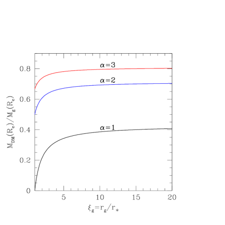
Figure 1.— Ratio between the dark mass and the total mass of JJ models (eq. 28), within a sphere of radius $r=R_{\rm e}\simeq 0.75r_{*}$, as a function of $\xi_{\rm g}$, for the minimum halo case ($\alpha=1$, black), and two non-minimum halo cases ($\alpha=2$, blue; and $\alpha=3$, red). The dark mass fraction is zero for the one-component (stellar) model, obtained for $\xi_{\rm g}=1$ and $\alpha=1$.

For what concerns the radial profile of $\rho_{\rm DM}$, for $r\to\infty$, eq. (25) shows that $\rho_{\rm DM}\sim({\cal R}_{\rm g}\xi_{\rm g}-1)\rho_{*}\propto r^{-4}$, and so the densities of the dark matter and of the stars in the outer regions are proportional. For $r\to 0$, in non minimum-halo models $\rho_{\rm DM}\sim({\cal R}_{\rm g}/\xi_{\rm g}-1)\rho_{*}\propto r^{-2}$, while in the minimum-halo models $\rho_{\rm DM}\sim 2(1-1/\xi_{\rm g})s\rho_{*}\propto r^{-1}$, so that these latter models are centrally baryon-dominated, being $\rho_{*}\propto r^{-2}$. It is interesting to compare the dark halo profile of JJ models with the NFW profile, of total mass $M_{\rm{DM}}$, that we rewrite for $r<r_{\rm t}$ (the so-called truncation radius) as:

$$\rho_{\rm NFW}(r)={\rho_{\rm n}({\cal R}_{\rm g}-1)\over f(c)s(\xi_{\rm NFW}+s)^{2}},\quad f(c)=\ln(1+c)-{c\over 1+c},$$ (29)

where $\xi_{\rm NFW}\equiv r_{\rm NFW}/r_{*}$ is the NFW scale-length $r_{\rm NFW}$ in units of $r_{*}$, and $c\equiv r_{\rm t}/r_{\rm NFW}$. From the considerations above about the behavior of $\rho_{\rm DM}(r)$ at small and large radii, it follows that $\rho_{\rm DM}$ and $\rho_{\rm NFW}$ at small and large radii cannot in general be similar. However, in the case of the minimum-halo, near the center $\rho_{\rm DM}\propto r^{-1}$, and it can be proven that $\rho_{\rm DM}$ and $\rho_{\rm NFW}$ can be made identical for $r\to 0$ by fixing

$$\xi_{\rm NFW}=\sqrt{{\xi_{\rm g}\over 2f(c)}}$$ (30)

in eq. (29). Therefore, once a specific JJ minimum halo model is considered, eqs. (29)-(30) allow to determine the NFW profile that has the same total mass and central density profile as $\rho_{\rm DM}$. It turns out that the dark halo profiles of JJ minimum halo models are surprisingly well approximated by the NFW profile over a very large radial range, for realistic values of $\xi_{\rm NFW}$ and $c$ (CZ18).

3.2. Dynamics of the JJ models

CZ18 present and discuss the analytical solutions of the Jeans equations and all the dynamical properties of Osipkov-Merritt anisotropic JJ models with a central MBH of mass $M_{\rm BH}$, where the total gravitational potential is

$$\Phi_{\rm T}(r)=\Phi_{\rm g}(r)-{\Psi_{\rm n}\mu\over s}.$$ (31)

The radial component of the stellar velocity dispersion tensor is given by $\sigma_{\rm r}^{2}(r)=\sigma_{\rm g}^{2}(r)+\sigma_{\rm BH}^{2}(r)$, where $\sigma_{\rm g}$ indicates the contribution due to $\Phi_{\rm g}(r)$, and $\sigma_{\rm BH}$ the contribution due to the MBH. Under the assumption of Osipkov-Merritt anisotropy, $\sigma_{\rm g}(0)$ is coincident with that of the isotropic case (except for purely radial orbits), independently of the anisotropy radius $r_{\rm a}>0$, and is given by:

$$\sigma_{\rm g}^{2}(0)={\Psi_{\rm n}{\cal R}_{\rm g}\over 2\xi_{\rm g}}={\Psi_{\rm n}\alpha\over 2},$$ (32)

where in the last identity we use eq. (27), and restrict to $\xi_{\rm g}\geq 1$. Note that the value of $\sigma_{\rm g}(0)$ is therefore independent of $\xi_{\rm g}$, for $\xi_{\rm g}\geq 1$, and, in the minimum halo model, it is coincident with that of the one-component (purely stellar) Jaffe model. The leading term of the MBH contribution to $\sigma_{\rm r}$ near the center (except for the case of purely radial orbits, $r_{\rm a}=0$) coincides with the isotropic case independently of the Osipkov-Merritt anisotropy radius, with

$$\sigma_{\rm BH}^{2}(r)\sim{\Psi_{\rm n}\mu\over 3s};$$ (33)

at variance with $\sigma_{\rm g}(r)$, it diverges as $\mu/r$ for $r\to 0$. Therefore, in presence of the central MBH, $\sigma_{\rm r}$ is dominated by its contribution, and similarly is the projected velocity dispersion ($\sigma_{\rm gp}$).

In order to relate the models with observed quantities, it is helpful to consider the projected velocity dispersion in the central regions. CZ18 shows that for $r_{\rm a}>0$

$$\sigma_{\rm gp}(0)=\sigma_{\rm g}(0)$$ (34)

while, independently of the value of $r_{\rm a}\geq 0$

$$\sigma_{\rm BHp}^{2}(R)\sim{2\Psi_{\rm n}\mu\over 3\pi}{r_{*}\over R},$$ (35)

where $R$ is the radius in the projection plane. The two equations above determine a fiducial value for the radius ($R_{\rm inf}$) of the so-called sphere of influence. We define operationally $R_{\rm inf}$ as the distance from the center in the projection plane where the (galaxy plus MBH) projected velocity dispersion $\sigma_{\rm p}(R)$ equals a chosen fraction $\epsilon$ of the projected velocity dispersion of the galaxy in absence of the MBH. In practice, as $R_{\rm inf}<<r_{*}$, and in JJ models without MBH the velocity dispersion profile flattens to a constant value, we define

$$\sigma_{\rm p}(R)\simeq\sqrt{\sigma_{\rm BHp}^{2}(R_{\rm inf})+\sigma_{\rm gp}^{2}(0)}=(1+\epsilon)\sigma_{\rm gp}(0),$$ (36)

and from eqs. (34)-(35) one has:

$${R_{\rm inf}\over r_{*}}={4\xi_{\rm g}\mu\over 3\pi{\cal R}_{\rm g}\epsilon(2+\epsilon)}={4\mu\over 3\pi\alpha\epsilon(2+\epsilon)},$$ (37)

where the last identity holds for $\xi_{\rm g}\geq 1$. For realistic values of the parameters, $R_{\rm inf}$ is of the order of a few pc (see Sect. 5.1 for a more quantitative discussion).

As anticipated in the Introduction, a reasonable estimate of the gas temperature, supported by observations (e.g., Pellegrini 2011), is given by the stellar virial temperature $T_{\rm V}=<\mu>m_{p}\sigma_{\rm V}^{2}/3$. The definition of $\sigma_{\rm V}$ comes from the virial theorem that, for the stellar component, reads:

$$2K_{*}=-W_{\rm*g}-W_{\rm*BH},$$ (38)

where $K_{*}\equiv M_{*}\sigma_{\rm V}^{2}/2$ is the total kinetic energy of the stars, and

$$W_{\rm*g}=-4\pi G\int_{0}^{\infty}r\rho_{*}(r)M_{\rm g}(r)dr$$ (39)

is the interaction energy of the stars with the total gravitational field of the galaxy (stars plus dark matter), and finally

$$W_{\rm*BH}=-4\pi GM_{\rm BH}\int_{0}^{\infty}r\rho_{*}(r)dr$$ (40)

is the interaction energy of the stars with the central MBH. Note that $W_{\rm*BH}$ diverges, because the stellar density profile diverges near the origin as $r^{-2}$; instead, $W_{\rm*BH}$ converges for $\gamma$ models with $0\leq\gamma<2$. Since we will use $K_{*}$ to evaluate the gas temperature over the whole body of the galaxy (where the MBH effect is negligible), we only consider $W_{\rm*g}$ in the determination of $\sigma_{\rm V}$. Therefore $\sigma_{\rm V}^{2}\equiv-W_{\rm*g}/M_{*}$, where from CZ18:

$$W_{\rm*g}=-\Psi_{\rm n}M_{*}{\cal R}_{\rm g}{\widetilde{W}}_{\rm g},\quad{\widetilde{W}}_{\rm g}={\xi_{\rm g}-1-\ln\xi_{\rm g}\over(\xi_{\rm g}-1)^{2}},$$ (41)

and ${\widetilde{W}}_{\rm g}(1)=1/2$. It follows that $\sigma_{\rm V}^{2}=\Psi_{\rm n}{\cal R}_{\rm g}{\widetilde{W}}_{\rm g}=\Psi_{\rm n}\alpha{\cal F}_{\rm g}(\xi_{\rm g})$, where we introduced the function ${\cal F}_{\rm g}(\xi_{\rm g})\equiv\xi_{\rm g}{\widetilde{W}}_{\rm g}$. Note that ${\cal F}_{\rm g}(\xi_{\rm g})$ increases from ${\cal F}_{\rm g}(1)=1/2$ to ${\cal F}_{\rm g}(\infty)=1$. In practice, at fixed $\alpha$ and increasing $\xi_{\rm g}$, eq. (27) dictates that ${\cal R}_{\rm g}$ increases to arbitrarily large values, but since ${\cal F}_{\rm g}\to 1$, then $W_{\rm*g}$ and $\sigma_{\rm V}$ (and so the mass-weighted squared escape velocity) remain limited. Physically, this is due to the fact that more massive halos are necessarily more and more extended, due to the request for positivity in eq. (26), with a compensating effect on the depth of the total potential. Moreover, from eqs. (32) and (34) it follows that $\sigma_{\rm V}^{2}=2{\cal F}_{\rm g}(\xi_{\rm g})\sigma_{\rm gp}^{2}(0)$, so that in JJ models without MBH, $\sigma_{\rm V}$ is just proportional to the stellar central projected velocity dispersion, and the proportionality constant is a function of $\xi_{\rm g}$ only, with $\sigma_{\rm V}=\sigma_{\rm gp}(0)$ for $\xi_{\rm g}=1$.

Table 1List of parameters

Symbol	Description
Galaxy structure:
$M_{\rm g}$	total mass
$M_{*}$	stellar mass
$M_{\rm BH}$	central MBH mass
$r_{\rm g}$	total density scale-length
$r_{*}$	stellar density scale-length
$\sigma_{\rm V}$	stellar virial velocity dispersion
$T_{\rm V}$	stellar virial temperature
$\mu$	$M_{\rm BH}/M_{*}$
$\xi_{\rm g}$	$r_{\rm g}/r_{*}$
${\cal R}_{\rm g}$	$M_{\rm g}/M_{*}$
	($=\alpha\xi_{\rm g}$, $\xi_{\rm g}\geq 1$, $\alpha\geq 1$)
Accretion flow:
$T_{\infty}$	temperature ($=\beta T_{\rm V}$, $\beta>0$)
$c_{\infty}$	sound velocity
$r_{\rm B}$	Bondi radius
$r_{\rm min}$	sonic radius
$\dot{M}_{\rm t}$	mass accretion rate
${\cal M}$	Mach number
$\lambda_{\rm t}$	critical accretion parameter
${\cal R}$	$M_{\rm g}/M_{\rm BH}$
$\xi$	$r_{\rm g}/r_{\rm B}$
$x_{\rm min}$	$r_{\rm min}/r_{\rm B}$
$\beta_{\rm c}$	critical $\beta$ ($=3/(2{\cal F}_{\rm g}$))

4. Linking stellar dynamics to fluidodynamics

In the general solution of CP17, once that the parameters $\cal R$ and $\xi$ in eq. (12) are assigned, and the Jaffe structural scales $M_{\rm g}$ and $r_{\rm g}$ characterizing the total galactic potential are chosen, the gas temperature $T_{\infty}$ remains fixed, because $\xi=r_{\rm g}/r_{\rm B}$. Therefore, generic values of $\xi$ can easily correspond to unrealistic values of the gas temperature. Clearly, JJ models offer an interesting possibility: as the dynamical properties of the stellar component of the galaxy can be analytically calculated once the total potential (due to stars, dark matter and central MBH) is assigned, the Virial Theorem for the stellar component can be used to compute the virial “temperature” $T_{\rm V}$ of the stars, a realistic proxy for the gas temperature $T_{\infty}$; then, the CP17 solution for the accreting gas in the total Jaffe potential of given $T_{\rm V}$ can be built. In practice, the idea is to self-consistently “close” the model, determining a fiducial value for the gas temperature as a function of the galaxy model hosting accretion. In this approach, the steps to build an accretion solution are: 1) choose $M_{*}$, $r_{*}$, $\mu$, ${\cal R}_{\rm g}$ and $\xi_{\rm g}$ for a realistic galactic model; 2) obtain the gas virial temperature $T_{\rm V}$; 3) derive ${\cal R}$ and $\xi$ to be used in the Bondi problem, and construct the corresponding CP17 solution.

Suppose the galaxy parameters in the first step are given. Then, for assigned ${\cal R}_{\rm g}$, $\xi_{\rm g}$ and $\mu$, the parameter ${\cal R}$ in the accretion solution is obtained from eqs. (12) and (21)-(22) as

$${\cal R}={{\cal R}_{\rm g}\over\mu}={\alpha\xi_{\rm g}\over\mu},$$ (42)

where the last expression depends on the fact that we restrict to the case $\xi_{\rm g}\geq 1$. Since $\mu\approx 10^{-3}$, and ${\cal R}_{\rm g}$ is expected (say) in the range $1\div 20$, the ${\cal R}$ values fall in the range $10^{3}\div 10^{4}$ (see also Sect. 5.1 for a more quantitative discussion).

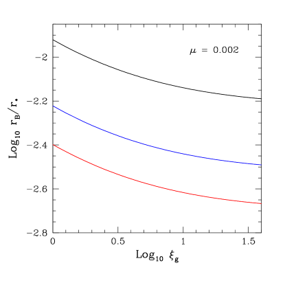
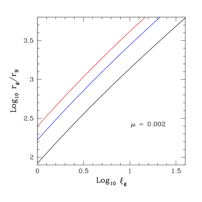
Figure 2.— Relevant scale-lengths of the isothermal accretion solution in JJ models, as a function of $\xi_{\rm g}=r_{\rm g}/r_{*}$. A MBH-to-galaxy stellar mass ratio $\mu=2\times 10^{-3}$ is assumed, and $T_{\infty}=\beta T_{\rm V}$. Top left: the ratio $r_{\rm B}/r_{*}$ from eq. (44) with $\beta=1$ and $\alpha=1,2,3$, following the color scheme as in Figure 1. Top right: ratio $r_{\rm B}/R_{\rm inf}$ of the Bondi radius to the radius of the sphere of influence of the MBH, $R_{\rm inf}$, for $\epsilon=0.5$ from eqs. (37) and (44), with $\beta=1$. Note that this ratio is independent of $\alpha$ and $\mu$. Bottom left: the parameter $\xi=r_{\rm g}/r_{\rm B}$ from eq. (46) with $\beta=1$ and $\alpha=1,2,3$. Bottom right: ratio $r_{\rm min}/r_{*}$ for $\alpha=1$ and $\beta=1,3/2,2,3$: for large values of ${\cal R}$ and $\beta<\beta_{\rm c}$ the ratio is almost independent of $\alpha$ but strongly dependent on gas temperature, as follows from eqs. (44), (47) and (48). Solid dots ($r_{\rm min}/r_{*}\simeq 13.84,0.011,0.0026$) mark the position of the sonic radius for the minimum halo case with $\xi_{\rm g}=20$.

From eq. (12), the second parameter ($\xi$) characterizing the accretion solution requires the computation of the Bondi radius $r_{\rm B}$, and then of the gas temperature $T_{\infty}$; we choose $T_{\infty}=\beta T_{\rm V}$, with $\beta>0$ a dimensionless parameter. Thus the isothermal sound speed is given by:

$$c_{\infty}^{2}={kT_{\infty}\over<\mu>m_{\rm p}}={\beta\sigma_{\rm V}^{2}\over 3},$$ (43)

and from eqs. (3) and (41) the Bondi radius reads:

$${r_{\rm B}\over r_{*}}={3\mu\over\alpha\beta{\cal F}_{\rm g}},\quad{\cal F}_{\rm g}\equiv\xi_{\rm g}{\widetilde{W}}_{\rm g}(\xi_{\rm g}).$$ (44)

From the behavior of the function ${\cal F}_{\rm g}(\xi_{\rm g})$, it follows that at fixed $\alpha$ and $\beta$ one has:

$${3\mu\over\alpha\beta}\leq{r_{\rm B}\over r_{*}}\leq{6\mu\over\alpha\beta},$$ (45)

where the lower limit is obtained for $\xi_{\rm g}\to\infty$, and the upper limit for $\xi_{\rm g}=1$; in this latter case, $\alpha=1$ gives the value of $r_{\rm B}/r_{*}$ in a one-component (stellar) Jaffe galaxy. As expected, $r_{\rm B}$ decreases for increasing $\alpha$, $\beta$ and $\xi_{\rm g}$, i.e., for increasing $T_{\infty}$. Figure 2 (top left panel) shows the trend of $r_{\rm B}/r_{*}$ with $\xi_{\rm g}$, in the minimum halo case ($\alpha=1$), and for $\alpha=2$ and $3$, when $\beta=1$ and $\mu=0.002$. Therefore, in a real galaxy with $r_{*}$ of the order of a few kpc, and with a gas temperature of the order of $T_{\rm V}$, $r_{\rm B}$ is of the order of tens of pc (see also Sect. 5.1 for a more quantitative discussion). As an additional information on $r_{\rm B}$, in Fig. 2 (top right panel) we show the trend of $r_{\rm B}/R_{\rm inf}$ with $\xi_{\rm g}$, for $\beta=1$; note that from eqs. (37) and (44), the ratio is independent of $\alpha$ and $\mu$, so that only one curve is plotted; higher values of $\beta$ correspond to smaller values of $r_{\rm B}$.

Using eqs. (44) and (12), we finally obtain the expression

$$\xi={\alpha\beta\xi_{\rm g}{\cal F}_{\rm g}\over 3\mu}={{\cal R}\beta{\cal F}_{\rm g}\over 3}.$$ (46)

It follows that $\xi\to\alpha\beta/(6\mu)$ for $\xi_{\rm g}\to 1$, while it grows without bound for $\xi_{\rm g}\to\infty$, as $\xi\sim\alpha\beta\xi_{\rm g}/(3\mu)$. In practice, at variance with the general cases in KCP16 and CP17, now ${\cal R}$ and $\xi$ are linked, and increasing values of ${\cal R}$ correspond to increasing values of $\xi$. The list of all parameters introduced in this work is given in Table 1. Figure 2 (bottom left panel) shows the trend of $\xi$ with $\xi_{\rm g}$, in the minimum halo case ($\alpha=1$), and for $\alpha=2$ and $3$, and $\beta=1$; $r_{\rm B}$ is of the order of $10^{-3}r_{\rm g}$; higher values of $\beta$ correspond to larger values of $\xi$.

Having obtained the expressions for ${\cal R}$ and $\xi$ as a function of the model parameters, a few considerations are in order. The first is that in JJ models isothermal accretion is always possible in absence of a central MBH and $\beta=1$, because the accretion condition in eq. (17) is automatically satisfied by the virial temperature of the stellar component, when $T_{\infty}=T_{\rm V}$. By allowing for a $T_{\infty}>T_{\rm V}$, it is easy to show that Bondi isothermal accretion in absence of a central MBH (or when $\chi=0$) is possible in JJ models only for gas temperatures lower than a critical value, i.e. only for $\beta\leq\beta_{\rm c}\equiv 3/(2{\cal F}_{\rm g})$. From the behavior of ${\cal F}_{\rm g}$ it follows that $3/2\leq\beta_{\rm c}\leq 3$, where the lower limit corresponds to $\xi_{\rm g}\to\infty$ and the upper limit to $\xi_{\rm g}=1$. The second is that from eq. (46) the ratio ${\cal R}/\xi=2\beta_{\rm c}/\beta$ appearing in the definition of $f(x)$ in eq. (13), depends on $\beta$ and $\xi_{\rm g}$ only, and it shows that for very large values of $\beta$ the problem reduces to the classical Bondi accretion.

The critical value $\beta_{\rm c}$ plays an important role also in models with a central MBH, determining a particular temperature at which there is a sudden transition in the position of the sonic radius. In fact, the location of $r_{\rm min}$ in terms of the scale-length $r_{*}$, is given by

$${r_{\rm min}\over r_{*}}=x_{\rm min}(\chi,{\cal R},\xi)\,{r_{\rm B}\over r_{*}},$$ (47)

where $x_{\rm min}$ is given by eq. (15), and can be easily computed analytically once ${\cal R}$ and $\xi$ are determined. Figure 2 (bottom right panel) shows $r_{\rm min}/r_{*}$ as a function of $\xi_{\rm g}$, for $\alpha=1$ and different values of $\beta$. The most relevant feature is the considerable variation in the position of $r_{\rm min}$, from very external to very inner regions, for $\beta$ increasing. Equation (47) shows that $r_{\rm min}$ is determined by the combined behavior of two functions, namely $x_{\rm min}$ and $r_{\rm B}/r_{*}$; we now focus on $x_{\rm min}$, having already established that $r_{\rm B}\propto 1/\beta$, and thus the large variation of $r_{\rm min}$ can only in part be due to the dependence of $r_{\rm B}$ on $\beta$. Instead, from eqs. (15), (42) and (46), for ${\cal R}\to\infty$ and fixed $\beta$, $x_{\rm min}$ is given by:

$$x_{\rm min}\sim\begin{cases}\displaystyle{{{\cal R}\;(1-\beta/\beta_{\rm c})\over 2},\quad\beta<\beta_{\rm c},}\\ \displaystyle{{\sqrt{\chi{\cal R}}\over 2},\quad\beta=\beta_{\rm c},}\\ \displaystyle{{\chi\over 2(1-\beta_{\rm c}/\beta)},\quad\beta>\beta_{\rm c}.}\end{cases}$$ (48)

Note that the limit ${\cal R}\to\infty$ describes models with increasing $\alpha$ at fixed $\mu$ and $\xi_{\rm g}$, or with increasing $\xi_{\rm g}$ at fixed $\alpha$ and $\mu$, or a vanishing MBH mass at fixed $\alpha$ and $\xi_{\rm g}$. As in the present models $\alpha\geq 1$, $\xi_{\rm g}\geq 1$ and $\mu=0.002$, then ${\cal R}$ is quite large, and the asymptotic trends in eq. (48) already provide a reasonable approximation of the true behavior, that is increasingly better for large values of $\alpha$ and $\xi_{\rm g}$, and small values of $\mu$. Of course, an independent check of the first two expressions above can be obtained by recovering them from the exact eq. (16) (pertinent to a Jaffe galaxy with $M_{\rm BH}=0$), by using eqs. (42) and (46) for vanishing MBH mass, i.e., $\mu\to 0$ and ${\cal R}\to\infty$, and $\beta\leq\beta_{\rm c}$.

Qualitatively, eq. (48) shows that for $\beta<\beta_{\rm c}$, $x_{\rm min}$ increases as ${\cal R}$. Instead, for $\beta>\beta_{\rm c}$, $x_{\rm min}$ is independent of ${\cal R}$, and for very large values of the gas temperature tends to $\chi/2$, the limit value of classical Bondi accretion with electron scattering (e.g., CP17, eq. 25). As Fig. 3 shows, even a moderate increase in the gas temperature produces a sudden decrease in the value of $x_{\rm min}$. A numerical investigation of polytropic accretion in JJ models shows that $x_{\rm min}$ suddenly drops to values $\lesssim 1$, as $\gamma$ increases with respect to the isothermal case. This behavior is reminiscent of the sudden transition of $x_{\rm min}$ from external to internal regions in Hernquist galaxies, discussed in CP17; in this case the transition is due to the existence, for $\gamma>1$, of two minima for the polytropic function $f(x)$ of the Jaffe potential (as obtained inserting eq. 11 in eq. 47 in KCP16). In the polytropic Hernquist case, the two minima can be present also in the isothermal case (CP17, Appendix B.2), while for the Jaffe potential in the isothermal case there is only one minimum, given in eq. (15).

It is now easy to explain the behavior of the curves in Fig. 2 (bottom right panel), where several cases of eq. (47) are plotted. For example, from the first identity in eq. (48) and eqs. (42)-(44), eq. (47) predicts that for ${\cal R}\to\infty$ and $\beta<\beta_{\rm c}$, we have $r_{\rm min}/r_{*}\sim\xi_{\rm g}(\beta_{\rm c}/\beta-1)$, so that for $\xi_{\rm g}\to\infty$ and $\beta=1$, it results $r_{\rm min}/r_{*}\sim\xi_{\rm g}/2$, while for $\xi_{\rm g}=1$ and large values of $\alpha/\mu$, one has $r_{\rm min}\approx 2r_{*}$. For $T_{\infty}$ corresponding to the range $3/2\leq\beta\leq 3$, there is a transition value of $\xi_{\rm g}$ such that, for larger $\xi_{\rm g}$, $\beta_{\rm c}$ drops below the adopted $\beta$, and the third expression in eq. (48) applies. In these cases the sonic radius moves to the central regions, with $r_{\rm min}/r_{*}\sim\chi\mu/[\alpha(\beta/\beta_{\rm c}-1)]$.

Figure 3.— Position of $x_{\rm min}$ as a function of the temperature parameter $\beta$, for $\mu=0.002$ and for three minimum halo models ($\alpha=1$), with $\xi_{\rm g}=1,3,20$; these correspond to critical values of the temperature given by $\beta_{\rm c}\simeq 3,2.2,1.7$, respectively (solid dots). The values of $x_{\rm min}$ are reproduced remarkably well by the asymptotic expressions in eq. (48).

Finally, Fig. 4 shows the trend of $\lambda_{\rm t}$ as a function of $\xi_{\rm g}$, for $\alpha=1,2,3$ and, when $\alpha=1$, for different gas temperatures as determined by the $\beta$ value (dotted lines). In analogy with eq. (48), an asymptotic analysis shows that in the limit of ${\cal R}\to\infty$,

$$\lambda_{\rm t}\sim\begin{cases}\displaystyle{{{\cal R}^{2}\;(1-\beta/\beta_{\rm c})^{2-{2\beta_{\rm c}\over\beta}}\over 4\sqrt{e}},\quad\beta<\beta_{\rm c},}\\ \displaystyle{{{\cal R}^{2}\over 4\sqrt{e}},\quad\beta=\beta_{\rm c},}\end{cases}$$ (49)

and for simplicity we do not report the expression of $\lambda_{\rm t}$ for $\beta>\beta_{\rm c}$, that however can be easily calculated. For fixed ${\cal R}$ and $\chi$, very large $\beta$ correspond to $\lambda_{\rm t}\sim\chi^{2}\lambda_{\rm cr}$, in accordance with the classical case (KCP16, CP17). Equation (49) nicely explains the values and the trend of $\lambda_{\rm t}$ with $\xi_{\rm g}$ and $\alpha$, in particular the almost perfect proportionality of $\lambda_{\rm t}$ to $\alpha^{2}\xi_{\rm g}^{2}$. From eq. (14), this implies that, for the same boundary conditions, the true accretion rate $\dot{M}_{\rm t}$ for increasing $\xi_{\rm g}$ becomes much larger than $\dot{M}_{\rm B}$, the rate in sole presence of the MBH.

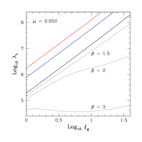
Figure 4.— The critical accretion parameter $\lambda_{\rm t}$ as a function of $\xi_{\rm g}$, for the miminum halo case $\alpha=1$ (black), and $\alpha=2,3$ (blue and red), and $\chi=1$ and $\beta=1$. The dotted curves refer to $\alpha=1$ and three different values of $\beta$.

5. Two applications

We present here two applications of the results above. The first is a practical illustration of how to determine the main parameters describing the galactic structure, and the gas accretion in it, for JJ models (see Table 1). One will see how very reasonable values for the main structural properties can be obtained, and then realistic galaxy models can be built. The second application considers the deviation from the true value of the mass accretion derived using the density along the accretion solution in JJ galaxies, and the framework of classical Bondi theory.

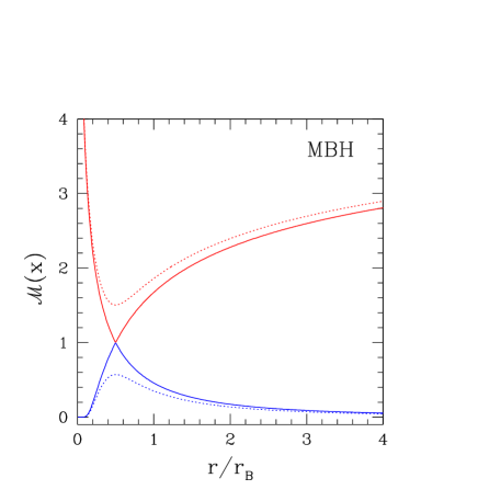
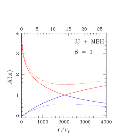
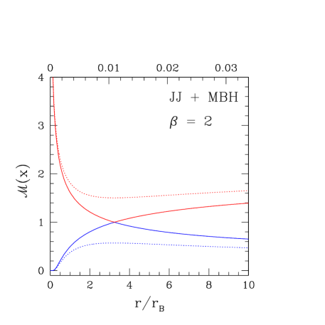
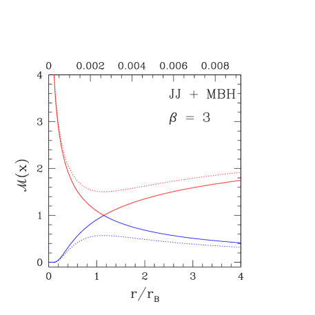
Figure 5.— Mach number profiles as a function of $x=r/r_{\rm B}$, for isothermal Bondi accretion (with $\chi=1$). The top left panel refers to classical Bondi accretion, and the other panels refer to accretion in a JJ galaxy model, plus a central MBH, with $\mu=2\times 10^{-3}$, ${\cal R}_{\rm g}=\xi_{\rm g}=20$, and $\beta=1,2,3$; the scale on the top gives the variable $r/r_{*}$. The subsonic regime is plotted in blue, the supersonic one in red. Solid lines show the two critical solutions, dotted lines show two subcritical solutions (with $\lambda=0.8\lambda_{\rm cr}$ in the top left panel, and $\lambda=0.8\lambda_{\rm t}$ in the others).

5.1. Accretion in realistic galaxy models

Here we show how to build JJ galaxy models with the main observed properties of real galaxies, and how to derive the corresponding parameters for isothermal accretion.

The first step consists of the determination of the stellar component of the JJ galaxy. This is done via the choice of two main galaxy properties, for example the effective radius $R_{\rm e}$ and the stellar projected velocity dispersion $\sigma_{\rm gp}(0)$. For JJ models $\sigma_{\rm gp}(0)=\sigma_{\rm g}(0)$, and $\sigma_{\rm g}(r)$ is quite flat at the center; thus $\sigma_{\rm gp}(0)$ is very close to the emission-weighted projected stellar velocity dispersion, within a small fraction of $R_{\rm e}$ (as typically given by observations). For chosen $R_{\rm e}$ and $\sigma_{\rm gp}(0)$, then, one has $r_{*}\simeq 1.34R_{\rm e}$ [see below eq. (20)], and then $M_{*}$, from eqs. (32) and (21) once a value for $\alpha\geq 1$ is fixed. The central MBH enters the problem via a choice for $\mu$, that here we take to be $\mu=2\times 10^{-3}$ (e.g., Kormendy & Ho 2013). Then the radius of influence $R_{\rm inf}$ can be evaluated from eq. (37). As an example, for a choice of $R_{\rm e}=5$ kpc, and $\sigma_{\rm gp}(0)=210$ km s^-1, one has $r_{*}\simeq 6.7$ kpc, $\alpha M_{*}\simeq 1.38\times 10^{11}$ M_⊙, and $R_{\rm inf}\simeq 4.6/\alpha$ pc, for a fiducial $\epsilon=0.5$.

The second step consists of the determination of the parameters ${\cal R}_{\rm g}$ and $\xi_{\rm g}$ that fix the total density distribution of the galaxy, and in particular its total potential. Since ${\cal R}_{\rm g}=\alpha\xi_{\rm g}$, we can only fix either ${\cal R}_{\rm g}$ or $\xi_{\rm g}$. It may be convenient to fix $\xi_{\rm g}$, for the following reason. A detailed dynamical modeling of stellar kinematical data for galaxies of the local universe has shown that the dark matter fraction within $R_{\rm e}$ is low (e.g., Cappellari 2016). To fit with this result, one can use eq. (28), that relates $\xi_{\rm g}$ and the dark matter fraction within any radius $r$; thus, for the desired (low) value of the dark matter fraction, $\xi_{\rm g}$ remains determined. Figure 1 shows that the ratio $M_{\rm{DM}}(R_{\rm e})/M_{\rm g}(R_{\rm e})$ is always in the range determined by the dynamical modeling, for $\alpha=1$. The figure also shows that, for $\xi_{\rm g}\gtrsim 5$, the dark matter fraction within $r=R_{\rm e}$ is quite independent of $\xi_{\rm g}$. This means that a certain freedom remains in the choice of $\xi_{\rm g}$, and we can further constrain it from other considerations. If $\alpha=1$, we may require that the scale-length of the dark halo ($r_{\rm NFW}$) is larger than that of the stars (i.e., $\xi_{\rm NFW}>1$). For example a value of the concentration parameter $c\simeq 10$, as predicted for galaxies of the local universe (e.g., Dutton & Macciò 2014), gives $\xi_{\rm NFW}=2.6$ for $\xi_{\rm g}=20$ [eq. (30)]. Finally, one recovers the stellar virial velocity dispersion $\sigma_{\rm V}^{2}=2{\cal F}_{\rm g}(\xi_{\rm g})\sigma_{\rm gp}^{2}(0)$, and then $T_{\rm V}$ from $\sigma_{\rm V}^{2}$. Since ${\cal F}_{\rm g}(\xi_{\rm g})$ varies only by a factor of two for $\xi_{\rm g}=1$ to $\infty$, then in turn $T_{\rm V}$ varies at most by a factor of two. For $\xi_{\rm g}=20$, one has $\sigma_{\rm V}\simeq 280$ km s^-1 and $T_{\rm V}\simeq 2.0\times 10^{6}$ K (for $<\mu>=0.6$).

Having completely determined the galaxy structure with the choice of two observed quantites, $R_{\rm e}$ and $\sigma_{\rm gp}(0)$, and three parameters ($\mu$, $\alpha$, $\xi_{\rm g}$), the next step consists in the determination of the accretion properties. These are all fixed, once the galaxy structure is fixed; only the gas temperature needs to be chosen. The first parameter describing accretion is ${\cal R}$, obtained from eq. (42). The second parameter is $\xi$, that comes from eq. (46), once the parameter $\beta$ is fixed in eq. (43). With the choice of this last parameter, i.e., with the choice of $T_{\infty}$, all the accretion properties are finally determined analytically, in particular the gas sound speed $c_{\infty}$ [eq. (43)], the Bondi radius $r_{\rm B}$ [eqs. (3) and (44)], the sonic radius $r_{\rm min}$ [eqs. (15) and (47)], the critical accretion parameter $\lambda_{\rm t}$ [as described below eq. (15)], and finally the Mach number profile ${\cal M}$ [eq. (18)]. As an example, for the galaxy model considered, for $\alpha=1$, $\beta=1$ and $\xi_{\rm g}=20$, one has ${\cal R}=10^{4}$, $r_{\rm B}\simeq 45$ pc, $\xi\simeq 2.96\times 10^{3}$, $r_{\rm min}\simeq 93$ kpc, and $\lambda_{\rm t}\simeq 5.23\times 10^{7}$. Instead, changing only the gas temperature to $\beta=2$, one has ${\cal R}$ unchanged, $r_{\rm B}\simeq 23$ pc, $\xi\simeq 5.91\times 10^{3}$, $r_{\rm min}\simeq 73$ pc, and $\lambda_{\rm t}\simeq 2.85\times 10^{6}$.

Figure 5 shows the Mach number profiles for accretion on a MBH (the classic Bondi problem), and on a MBH at the center of a JJ model, for the minimum halo case and three values of $\beta$. For the three galaxy models the top axis gives the radial scale in terms of $r/r_{*}$. Again it is apparent how a modest increase in the gas temperature produces a dramatic decrease of $r_{\rm min}$. Figure 6 shows a comparison between the gas velocity profile and the stellar velocity dispersion profile, for the JJ models in Fig. 5. Notice that near the center $\sigma_{\rm BH}\sim r^{-1/2}$ and ${\cal M}\sim r^{-1/2}$ so that their ratio is a constant; it can be easily shown that this constant is ${\sqrt{6\chi}}$, independently of $\alpha$, $\beta$, $\xi_{\rm g}$, ${\cal R}_{\rm g}$ and $\mu$. In principle, then, the value of $\sigma_{\rm BH}$ close to the center of a galaxy is a proxy for the (isothermal) gas inflow velocity.

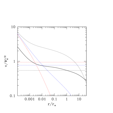
Figure 6.— Accretion velocity profile for the gas (dotted) and isotropic stellar velocity dispersion profile (solid), both normalized to $\sqrt{\Psi_{\rm n}}$, for the minimum halo model with ${\cal R}_{\rm g}=\xi_{\rm g}=20$. The accretion solutions correspond to $\beta=1,2,3$ and are given by the black, blue and red dotted lines, respectively. The horizontal dotted lines mark the corresponding values of $c_{\infty}/\sqrt{\Psi_{\rm n}}$. For each $\beta$ the intersection between the accretion velocity and the sound velocity marks the sonic point (bottom right panel in Fig. 2, solid dots).

5.2. The bias in estimates of the mass accretion rate

We investigate here the use of the classical Bondi solution in problems involving accretion on MBHs residing at the center of galaxies. This use is common in the interpretation of observational results, in numerical investigations, or in cosmological simulations (see Sect. 1). In many such studies, when the instrumental resolution is limited, or the numerical resolution is inadequate, an estimate of the mass accretion rate is derived using the classical Bondi solution, taking values of temperature and density measured at some finite distance from the MBH. This procedure clearly produces an estimate that can depart from the true value, even when assuming that accretion fulfills the hypotheses of the Bondi model (stationariety, spherical symmetry, etc.). KCP16 developed the analytical set up of the problem for generic polytropic accretion, with the inclusion of the effects of radiation pressure and of a galactic potential; they also investigated numerically the size of the deviation for Hernquist galaxies. CP17 presented a detailed exploration of the deviation for isothermal accretion in one-component Jaffe and Hernquist galaxies was done by CP17. Here we consider the more realistic case of two-component JJ models, in the isothermal case, exploiting the fully analytical character of JJ models.

We first consider the deviation of the estimate of the mass accretion rate for the classical Bondi solution, when taking values of temperature and density measured at some finite distance from the MBH. For assigned values of $\rho_{\infty}$, $T_{\infty}$, $\gamma$ and $M_{\rm BH}$, the Bondi radius $r_{\rm B}$ and the critical accretion rate $\dot{M}_{\rm B}$ are given by eq. (3) and by eq. (5) with $\lambda=\lambda_{\rm cr}$. If one inserts in these equations the values of $\rho(r)$ and $T(r)$ at a finite distance $r$ from the MBH, taken along the classical Bondi solution, and considers them as “proxies” for $\rho_{\infty}$ and $T_{\infty}$, then an estimated value for the accretion radius ($r_{\rm e}$) and mass accretion rate ($\dot{M}_{\rm e}$) is obtained:

$$r_{\rm e}(r)\equiv{GM_{\rm BH}\over c_{\rm s}^{2}(r)},\quad\dot{M}_{\rm e}(r)\equiv 4\pi r_{\rm e}^{2}(r)\lambda_{\rm cr}\rho(r)c_{\rm s}(r).$$ (50)

The question is how much $r_{\rm e}$ and $\dot{M}_{\rm e}$ depart from the true values $r_{\rm B}$ and $\dot{M}_{\rm B}$, as a function of $r$. In the isothermal case the sound speed is constant, with $c_{\rm s}(r)=c_{\infty}$, and then $r_{\rm e}(r)=r_{\rm B}$, independently of the distance from the center at which the temperature is evaluated. Then $\dot{M}_{\rm e}(r)=4\pi r_{\rm B}^{2}\lambda_{\rm cr}\rho(r)c_{\infty}$; at infinity, $\dot{M}_{\rm e}=\dot{M}_{\rm B}$. At finite radii, instead

$${\dot{M}_{\rm e}(r)\over\dot{M}_{\rm B}}=\tilde{\rho}(x)={\lambda_{\rm cr}\over x^{2}{\cal M}(x)},$$ (51)

where the last identity comes from eq. (9), and ${\cal M}(x)$ is given in eq. (19) of CP17. The deviation of $\dot{M}_{\rm e}$ from $\dot{M}_{\rm B}$ then is just given by ${\tilde{\rho}(x)}$ at the radius $r$ where the “measure” is taken. Thus, $\dot{M}_{\rm e}$ gives an overestimate of $\dot{M}_{\rm B}$, and this overestimate becomes larger for decreasing $x$ (see Fig. 1 in KCP16, and Fig. 4 in CP17).

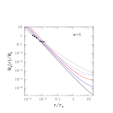
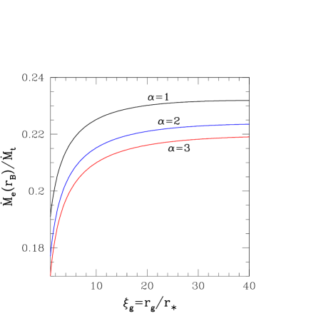
Figure 7.— Left: ratio between the estimate of the accretion rate $\dot{M}_{\rm e}$ and the true accretion rate $\dot{M}_{\rm t}$, from eq. (52), as a function of $r/r_{*}$, in the minimun halo case ($\alpha=1$), for $\chi=1$, $\beta=1$, and $\xi_{\rm g}=1$ (red), $\xi_{\rm g}=3$ (blue), and $\xi_{\rm g}=20$ (black). The dotted lines correspond to $\beta=3$, and the solid dots mark the position of the Bondi radius $r_{\rm B}$ in eq. (44). Right: the ratio $\dot{M}_{\rm e}/\dot{M}_{\rm t}$ evaluated at $r_{\rm B}$, as a function of $\xi_{\rm g}$, for three values of $\alpha$, and $\chi=1$, $\beta=1$. In both panels $\mu=0.002$.

In presence of a galaxy, the departure of $\dot{M}_{\rm e}(r)$ of eq. (50) from the true mass accretion rate $\dot{M}_{\rm t}=4\pi r_{\rm B}^{2}\lambda_{\rm t}\rho_{\infty}c_{\infty}$, is:

$${\dot{M}_{\rm e}(r)\over\dot{M}_{\rm t}}={\lambda_{\rm cr}\tilde{\rho}(x)\over\lambda_{\rm t}}={\lambda_{\rm cr}\over x^{2}{\cal M}(x)},$$ (52)

where $\rho(r)$ is taken along the solution for accretion within the potential of the galaxy, the last identity comes from eq. (19), and ${\cal M}(x)$ is given in eq. (18).

Figure 7 (left panel) shows the trend of $\dot{M}_{\rm e}/\dot{M}_{\rm t}$ with $r$. One sees that the use of $\rho(r)$ instead of $\rho_{\infty}$ leads to an overestimate for $r$ taken in the central regions, while $\dot{M}_{\rm e}(r)$ becomes an underestimate for $r\gtrsim$ a few$\times 10^{-3}r_{*}$. The radius marking the transition from the region in which there in an overestimate, to that where there is an underestimate, depends on the specific galaxy model. An important consequence of the results in Fig. 7 is that, for example, in numerical simulations not resolving $r_{\rm B}$, $\dot{M}_{\rm e}$ should be boosted by a large factor to approximate the true accretion rate $\dot{M}_{\rm t}$. Moreover, since $\dot{M}_{\rm e}/\dot{M}_{\rm t}$ increases steeply with $r$, this “boost factor” in turn also varies steeply with $r$. In the right panel of Fig. 7 we also show the bias measured at the Bondi radius as a function of $\xi_{\rm g}$. The panel indicates an underestimate by roughly a factor of 5.

It is instructive to find the reason for the trend of $\dot{M}_{\rm e}$ near the center and at large radii. From eq. (52) and the expansion of ${\cal M}$ for $x\to 0^{+}$ and for $x\to\infty$, one has:

$${\dot{M}_{\rm e}(r)\over\dot{M}_{\rm t}}\sim{\lambda_{\rm cr}\over\sqrt{2\chi}x^{3/2}},\quad x\to 0^{+},$$ (53)

and

$${\dot{M}_{\rm e}(r)\over\dot{M}_{\rm t}}\sim{\lambda_{\rm cr}\over\lambda_{\rm t}},\quad x\to\infty.$$ (54)

Therefore near the center $\dot{M}_{\rm e}/\dot{M}_{\rm t}\sim r^{-3/2}$, while at large radii, as in general $\lambda_{\rm t}>>\lambda_{\rm cr}$ (see Fig. 4), $\dot{M}_{\rm e}/\dot{M}_{\rm t}$ becomes very small.

6. Summary and conclusions

The classical Bondi accretion theory is the tool commonly adopted in many investigations where an estimate of the accretion radius and the mass accretion rate is needed. In this paper, extending the results of previous works (KCP16, CP17), we focus on the case of isothermal accretion in two-component galaxies with a central MBH, and with radiation pressure contributed by electron scattering in the optically thin regime. In CP17 it was shown that the radial profile of the Mach number, and the critical eigenvalue of the isothermal accretion problem, can be expressed analitycally in Jaffe and Hernquist potentials with a central MBH. Here we adopt the two-component JJ galaxy models presented in CZ18. These are made of a Jaffe stellar component plus a dark halo such that the total density is also described by a Jaffe profile; all the relevant dynamical properties of JJ models, including the solution of the Jeans equations for the stellar component, can be expressed analytically. Therefore, the results of CP17 and CZ18 give the opportunity of building a family of two-component galaxy models where all the accretion properties can be given analytically, and then explored in detail, with no need to resort to numerical studies. The main results of this work can be summarized as follows.

1) The parameters describing accretion in the hydrodynamical solution of CP17 (${\cal R}$ and $\xi$) have been linked to the galaxy structure. In particular, it is assumed that the isothermal gas has a temperature $T_{\infty}$ proportional to the virial temperature of the stellar component, $T_{\rm V}$. Then, simple formulas are derived relating the galactic properties (as the effective radius, $R_{\rm e}$, and the radius of influence of the MBH, $R_{\rm inf}$) with those describing accretion (as the Bondi radius $r_{\rm B}$, and the sonic radius $r_{\rm min}$). The critical accretion parameter $\lambda_{\rm t}$ is also expressed as a function of the galactic properties.

2) For realistic galaxy structures, $r_{\rm B}$ is of the order of a few$\times 10^{-3}r_{*}$, and $R_{\rm inf}$ is of the order of $\simeq 0.1r_{\rm B}$. For $T_{\infty}=T_{\rm V}$, the sonic radius $r_{\rm min}$ is of the order of a few $R_{\rm e}$. For moderately higher values of $T_{\infty}$, $r_{\rm min}$ suddenly drops to radii within $r_{\rm B}$. The same happens also for a small increase of the polytropic index above unity, and this behavior is reminiscent of the similar jump shown by $r_{\rm min}$ in Hernquist models, as discussed in CP17. As a consequence, accretion in JJ models can switch from being supersonic over almost the whole galaxy to being everywhere subsonic, except for $r\lesssim r_{\rm B}$. An explanation for this phenomenon is given.

3) As for the isothermal accretion in one-component Jaffe models, the determination of the critical accretion parameter involves the solution of a quadratic equation, and there is only one sonic point for any choice of the parameters describing the galaxy. In presence of the galaxy, $\lambda_{\rm t}$ is several orders of magnitude larger than without the galaxy. It is found that Bondi accretion in JJ models in absence of a central MBH (or when $\chi=0$) is possible, provided that $T_{\infty}$ is lower than a critical value and we derive the esplicit formula for it. This critical value depends only on $\xi_{\rm g}$, and is in the range $3/2\leq T_{\infty}/T_{\rm V}\leq 3$. It also determines the the jump in $r_{\rm min}$ in models with the central MBH.

4) We provide a few examples of accretion in realistic galaxy models, and present the resulting Mach number profiles, the trends of the accretion velocity and of the isotropic stellar velocity dispersion profiles.

5) We finally examine the problem of the deviation from the true value $\dot{M}_{\rm t}$ of an estimate of the mass accretion rate $\dot{M}_{\rm e}(r)$ obtained adopting the classical Bondi solution for accretion on a MBH, where the gas density and temperature at some finite distance from the center are inserted, as proxies for their values at infinity. The size of the departure of $\dot{M}_{\rm e}(r)$ from $\dot{M}_{\rm t}$, that is determined by the presence of the galaxy, is given as a function of the distance $r$ from the center. $\dot{M}_{\rm e}(r)$ overestimates $\dot{M}_{\rm t}$, if the gas density is taken in the very central regions, and underestimates $\dot{M}_{\rm t}$ if it is taken outside a few Bondi radii. This shows how sensitive to the model parameters is the determination of a physically based value for the so-called “boost factor” adopted in simulations, and that in general a universally valid prescription is impossible.

References

- Barai11 (2011) Barai, P., Proga, D., & Nagamine, K. 2011, MNRAS, 418, 591
- Barai12 (2012) Barai, P., Proga, D., & Nagamine, K. 2012, MNRAS, 424, 728
- Barai18 (2018) Barai, P., de Gouveia Dal Pino, E.M. 2018, MNRAS in press (arXiv:1807.04768)
- Beckmann (2018) Beckmann, R. S., Slyz, A., Devriendt, J. 2018, MNRAS 478, 995
- Bondi (1952) Bondi, H., 1952, MNRAS 112, 195
- Bu (2013) Bu, D.-F., Yuan, F., Wu, M., Cuadra, J. 2013, MNRAS 434, 1692
- Cappellari (2015) Cappellari, M., Romanowsky, A. J., Brodie, J. P., et al. 2015, ApJL, 804, L21
- Michele (2016) Cappellari, M. 2016, ARA&A 54, 597
- Cao (2016) Cao, X. 2016 ApJ 833, 30
- CdZvdM (1995) Carollo, M., van der Marel, R., & de Zeeuw, P.T. 1995, MNRAS 276, 1131
- Choi (2017) Choi, E., Ostriker, J.P.O., Naab, T., et al. 2017, MNRAS 844, 31
- C (1999) Ciotti, L. 1999, ApJ, 520, 574
- Ciotti (2012) Ciotti, L., Ostriker, J. P. 2012, in Hot Interstellar Matter in Elliptical Galaxies, Vol. 378, eds. D.-W. Kim and S. Pellegrini (New York: Springer), 83
- CLR (1996) Ciotti, L., Lanzoni, B., & Renzini, A. 1996, MNRAS 282, 1
- CMdZ (2009) Ciotti, L., Morganti, L., & de Zeeuw, P.T. 2009, MNRAS 393, 491
- CP (2017) Ciotti, L., Pellegrini, S. 2017, ApJ 848, 29 (CP17)
- CZ (2018) Ciotti, L., & Ziaee Lorzad, A. 2018, MNRAS, 473, 5476 (CZ18)
- Dehnen (1993) Dehnen, W. 1993, MNRAS 265, 250
- DiMatteo (2008) Di Matteo, T., Colberg, J., Springel, V., Hernquist, L., Sijacki, D. 2008, ApJ 676, 33
- Dutton (2014) Dutton, A.A., Macciò, A.V., 2014, MNRAS 441, 3359
- Frank (1992) Frank, J., King, A. and Raine, D., 1992, Accretion power in astrophysics., Camb. Astrophys. Ser., Vol. 21, Cambridge University Press
- Gallo (2010) Gallo, E., et al. 2010, ApJ 714, 25
- Hernquist (1990) Hernquist, L., 1990, ApJ 356, 359
- Jaffe (1983) Jaffe, W., 1983, MNRAS 202, 995
- Kormendy (2013) Kormendy, J., Ho, L.C. 2013, ARA&A 51, 511
- Korol (2016) Korol, V., Ciotti, L., Pellegrini, S. 2016, MNRAS 460, 1188 (KCP16)
- Lusso (2011) Lusso, E., and Ciotti, L., 2011, A&A 525, 115
- Merritt (1985) Merritt D., 1985, AJ, 90, 1027
- Mosci (2013) Mościbrodzka, M., & Proga, D. 2013, ApJ 767, 156.
- Navarro (1997) Navarro, J. F., Frenk, C. S., White, S.D.M. 1997, ApJ 490, 493
- Park (2017) Park, K.-H., Wise, J.H., Bogdanović, T. 2017, ApJ 847, 70
- Pellegrini (2010) Pellegrini, S. 2010, ApJ 717, 640
- Pellegrini (2011) Pellegrini, S. 2011, ApJ 738, 57
- Rafferty (2006) Rafferty, D. A., McNamara, B. R., Nulsen, P. E. J., & Wise, M. W. 2006, ApJ 652, 216
- Ram (2018) Ramírez-Velasquez, J.M., Sigalotti, L. Di G., Gabbasov, R., Cruz, F., Klapp, J. 2018, MNRAS 477, 4308
- Sijacki (2007) Sijacki, D., Springel, V., Di Matteo, T., Hernquist, L. 2007, MNRAS 380, 877
- Tremaine (1994) Tremaine, S., Richstone, D. O., Byun, Y.-I., et al. 1994, AJ 107, 634
- Volonteri (2015) Volonteri, M., Capelo, P.R., Netzer, N., et al. 2015, MNRAS 449, 1470