A magnetic Hofstadter butterfly and its topologically quantized Hall conductance

Abstract

The energy spectrum of massless Dirac fermions in graphene under two dimensional periodic magnetic modulation having square lattice symmetry is calculated. We show that the translation symmetry of the problem is similar to that of the Hofstadter or TKNN problem and in the weak field limit the tight binding energy eigenvalue equation is indeed given by Harper Hofstadter hamiltonian. We show that due to its magnetic translational symmetry the Hall conductivity can be identified as a topological invariant and hence quantized. We thus extend the idea of Quantum Hall Effect to magnetically modulated two dimensional electron system. Finally we indicate possible experimental systems where this may be verified.

The Integer Quantum Hall effect (IQHE), one of the most fascinating phenomena in condensed matter physics and beyond, shows extremely precise quantization of magneto-transport (Hall conductivity) in a two dimensional electron gas (2DEG) placed in a transverse magnetic field. It was first discovered in a system with non-relativistic dispersion Klitzing ; Tsui ; Laughlin1 ; Halperin (Silicon MOSFET and semiconductor heterostructure), and subsequently in a 2DEG with relativistic dispersion Novoselov1 ; Kim realised in Graphene. In a seminal paper Thouless, Kohmoto, Nightingale, and den Nijs (TKNN) Thouless1 identified this quantized Hall conductance of a 2DEG in a transverse magnetic field and a strong periodic potential Hofstadter with a topological invariant Avron1 called first Chern number defined in the space of Bloch vectors. This remarkable idea not only explained the robust quantization of a transport quantity, but fundamentally modified the conventional understanding of band structure of transport. This idea was further significantly generalised when Haldane Haldane showed that such topological quantization of Hall conductivity can be achieved for a fully filled band even in the absence of a net magnetic field leading to anomalous quantum Hall Effect (AQHE). Haldane’s seminal work was further generalised in systems without any external magnetic field, that respect time reversal symmetry BHZ ; KM and lead to the discovery of present day Topological Insulators HK .

This letter considers two dimensional gas of massless Dirac fermions with relativistic dispersion, the charge carriers in monolayer graphene, in the presence of a periodically modulated transverse magnetic field. We show that such magnetic field is composed of two parts. One part corresponds to a uniform field, like that in a prototype quantum Hall system. The other part gives a periodic modulation which has zero net flux through each unit cell. Thus the second part gives qualitatively similar flux condition as in the Haldane’s problemHaldane leading to AQHE, but realised in a different lattice geometry as compared to Haldane’ s construction. Subsequently we write the resulting vector potential as a combination of the usual symmetric gauge vector potential for a uniform transverse field and a periodic vector potential for the modulated part, whose form we also explicitly construct. This decomposition enables us to identify that the magnetic translation operator Zak ; Fischbeck ; Florek for this problem is same as that in the TKNN Thouless1 problem.

This has interesting consequences. The corresponding hamiltonian is a perturbed form of the hamiltonian used in the classic Hofstadter problem Hofstadter . However here the periodicity comes entirely from magnetic modulation. We therefore address this as a magnetic Hofstadter problem. In tight-binding approximation and in the weak field limit we show that the problem is indeed Hofstadter-Harper equation. We analyse its spectrum. Finally the properties of the magnetic Bloch functions are used to show that the Hall conductivity stays quantised as in the TKNN problem and can be identified with the Chern number of a filled band. Thus our decomposition of magnetic field profile allows us to show the topological quantization of Hall conductivity for a generic magnetically modulated 2DEG.

The effect of periodic magnetic modulation in one Peeters ; Krakovsky and two dimension Chang ; Oh on a 2DEG has been considered earlier in a number of papers. They mostly explore the resulting band structure Peeters ; Krakovsky and the perturbation of Landau levels formed in a uniform magnetic field. Our decomposition of a general periodic magnetic modulation and the identification of the magnetic translation symmetry not only provides a unifying theoretical framework to these previous studies but also establishes a connection between conventional Quantum Hall effect and AQHE espoused in Haldane like models. We conclude the paper by indicating some physical systems where this prediction can be put to experimental test.

We consider the charge carriers in monolayer graphene in a transverse periodic magnetic field modulation (Fig. 1) given by

$$B\boldsymbol{\hat{z}}=\Big{[}B_{2}+(B_{1}-B_{2})\sum_{m,n}\Theta(R^{s}-r_{mn})\Big{]}\boldsymbol{\hat{z}}$$ (1)

in the $\boldsymbol{k}\cdot\boldsymbol{p}$ representation, described by the massless dirac hamiltonian

$$\hat{H}=v_{F}(\boldsymbol{\sigma}\cdot\boldsymbol{\Pi})$$ (2)

where $\boldsymbol{\Pi}=\boldsymbol{p}+\frac{e\boldsymbol{A}}{c}$ is the canonical momentum operator with $\boldsymbol{A}$ as the vector potential for field (1). $R^{s}$ is the radius of the circular region within each unit cell, $\boldsymbol{r}_{mn}=\boldsymbol{r}-\boldsymbol{R}_{mn}$ with $\boldsymbol{r}=x\boldsymbol{\hat{x}}+y\boldsymbol{\hat{y}}$. The lattice vector $\boldsymbol{R}_{mn}=ma\boldsymbol{\hat{x}}+na\boldsymbol{\hat{y}}$ and

$$\Theta(R^{s}-r_{mn}) = \begin{cases}1,~{}~{}\text{if}~{}\ r_{mn}\leq R^{s},\\ 0,~{}~{}\text{if}~{}\ r_{mn}>R^{s}\end{cases}$$ (3)

with $m,n\in I(-N_{max},+N_{max})$ and $a$ is the lattice constant. The step function modelling can be justified by assuming that the magnetic field gradient at the step is much sharper than the typical Fermi-wavelength of the electron Egger ; Peeters ; Alain ; Neetu . Such two dimensional periodic modulation corresponds to that of a square lattice and can be made using nanolithographic techniques expt1 ; Bader .

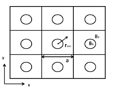
Figure 1: Monolayer Graphene under a two dimensional magnetic field array with inside circular regions with radius $R_{s}$ having $B_{1}\boldsymbol{\hat{z}}$ and that of outside having $B_{2}\boldsymbol{\hat{z}}$

Using Fourier theorem, the periodic magnetic field profile given by Eq. $(\ref{B})$ can be written as

$$\boldsymbol{B}=\sum_{\boldsymbol{G}}\boldsymbol{B}_{\boldsymbol{G}}e^{i\boldsymbol{G}.\boldsymbol{r}}=\boldsymbol{B}_{0}+\sum_{\boldsymbol{G}\neq 0}\boldsymbol{B}_{\boldsymbol{G}}e^{i\boldsymbol{G}.\boldsymbol{r}}$$ (4)

Here $\boldsymbol{G}$ is the reciprocal lattice vector of the periodic lattice, $\boldsymbol{B}_{0}=\boldsymbol{B}_{u}$ is the uniform magnetic field and is given by spatial average of the field given in Eqn. $(\ref{B})$. The residual periodic field is defined as $\boldsymbol{B}_{p}=\sum_{\boldsymbol{G}\neq 0}\boldsymbol{B}_{\boldsymbol{G}}e^{i\boldsymbol{G}.\boldsymbol{r}}$ that satisfies $\boldsymbol{\nabla}\cdot\boldsymbol{B}_{p}=0$ with net flux through the unit cell due to $\boldsymbol{B}_{p}$ is zero (for details see suppli ). This decomposition remains valid even for an arbitrary periodic modulation. Consequently if we apply uniform magnetic field $-\boldsymbol{B}_{u}$ to this system, under suitable condition this can realise Haldane like model Bruno ; Snyman . Now, following Brownbook it can be shown that there corresponds a periodic vector potential for the residual periodic field $\boldsymbol{B}_{p}$. Accordingly we can decompose the magnetic field and corresponding vector potential in uniform and periodic parts like

$$B\boldsymbol{\hat{z}}=B_{u}\boldsymbol{\hat{z}}+B_{p}\boldsymbol{\hat{z}}~{}\text{and}~{}\boldsymbol{A}(\boldsymbol{r})=\boldsymbol{A}_{u}(\boldsymbol{r})+\boldsymbol{A}_{p}(\boldsymbol{r})$$

with

$$B_{u} = \Big{[}B_{2}+\frac{(B_{1}-B_{2})\pi(R^{s})^{2}}{a^{2}}\Big{]}$$

$$B_{p} = \Big{[}\sum_{m,n}((B_{1}-B_{2})\theta(R^{s}-r_{mn}))$$ (5)

$$- \frac{(B_{1}-B_{2})\pi(R^{s})^{2}}{a^{2}}\Big{]}$$

$$\boldsymbol{A}_{u}(\boldsymbol{r}) = \frac{1}{2}\boldsymbol{B}_{u}\times\boldsymbol{r},~{}\text{Symmetric Gauge}$$

$$\boldsymbol{A}_{p}(\boldsymbol{r}) = \frac{1}{2}\sum_{m,n}\Big{[}(B_{p}^{mn}\boldsymbol{\hat{z}})\times(r_{mn}\boldsymbol{\hat{r}}_{mn})\Big{]}$$ (6)

where

$$B_{p}^{mn}=\begin{cases}\Big{[}(B_{1}-B_{2})-\frac{(B_{1}-B_{2})\pi(R^{s})^{2}}{a^{2}}\Big{]}\Theta(R^{s}-r_{mn}),\\ \text{if}\ r_{mn}\leq R^{s}\\ \\ (B_{2}-B_{1})\frac{\pi(R^{s})^{2}}{Na^{2}}\Theta(r_{mn}-R^{s}),~{}\text{otherwise}\end{cases}$$ (7)

To construct $\boldsymbol{A}_{p}(\boldsymbol{r})$, we considered single unit magnetic field profile $\Big{[}\frac{B_{2}}{N}+(B_{1}-B_{2})\Theta(R^{s}-r_{m,n})\Big{]}\boldsymbol{\hat{z}}$ for a specific $(m,n)$. The vector potential for such field can be found in azimuthal gauge using Stoke’s law. Superposing such units for all possible $(m,n)$ and doing suitable gauge transformation one gets $\boldsymbol{A}_{p}(\boldsymbol{r})$ (for details see suppli ).

With canonical momentum operator now defined as $\boldsymbol{\Pi}=\boldsymbol{p}+\frac{e}{c}(\boldsymbol{A}_{u}+\boldsymbol{A}_{p})$ , the eigenvalue equation for the hamiltonian in $(\ref{Ham1})$, is rewritten as

$$v_{F}\left[{\begin{array}[]{cc}0&\Pi_{x}-i\Pi_{y}\\ \Pi_{x}+i\Pi_{y}&0\\ \end{array}}\right]\begin{bmatrix}\psi^{a}_{k_{x},k_{y}}\\ \psi^{b}_{k_{x},k_{y}}\end{bmatrix}=E\begin{bmatrix}\psi^{a}_{k_{x},k_{y}}\\ \psi^{b}_{k_{x},k_{y}}\end{bmatrix}$$ (10)

Here the periodic vector potential $\boldsymbol{A}_{p}$ has the periodicity of the square lattice magnetic modulation. Thus the magnetic translation operator $M_{\boldsymbol{R}}$ corresponding to $\boldsymbol{\Pi}$ is same as the magnetic translation operator Zak ; Fischbeck ; Florek of an electron in periodic scalar potential of a square lattice and uniform transverse magnetic field. Explicitly

$$M_{\boldsymbol{R}}=exp{(\frac{i}{\hbar}\boldsymbol{R}.(\boldsymbol{p}-\frac{e\boldsymbol{A}_{u}}{c}))}$$ (11)

We note that by construction $[\boldsymbol{p}+\frac{e}{c}\boldsymbol{A}_{u},M_{\boldsymbol{R}}]=0$. Since the periodic part of the vector potential $\boldsymbol{A}_{p}(\boldsymbol{r}+\boldsymbol{R})=\boldsymbol{A}_{p}(\boldsymbol{r})$, we have $[\boldsymbol{A}_{p},M_{\boldsymbol{R}}]=0$. Thus the hamiltonian in (2) or in (10) commutes with $M_{\boldsymbol{R}}$ and and they have simultaneous eigenstates which are magnetic Bloch functions Zak2 . This result only depends on the periodicity of $\boldsymbol{A}_{p}$ and not on the explicit form (6). The significance of this result is that it is now possible to obtain the spectral properties as well as, using TKNN approach, the transport properties for the quasiparticles described by the hamiltonian (2).

To obtain the spectrum we use standard procedure of decoupling of Eq. (10) and get the eigenvalue equations for each sub-lattice. This becomes

$$\hat{H}_{G}(x,y)\psi_{\boldsymbol{k}}^{a,b}(x,y)=E^{2}\psi_{\boldsymbol{k}}^{a,b}(x,y)$$ (12)

with

$$\hat{H}_{G}=v_{F}^{2}((p+\frac{e}{c}A_{u})^{2}+V_{p}(\boldsymbol{r})+V_{np}(\boldsymbol{r}))$$ (13)

where $V_{p}(\boldsymbol{r})=\frac{e^{2}}{c^{2}}A_{p}^{2}+\frac{2e}{c}\boldsymbol{A}_{p}.\boldsymbol{p}+\hbar\frac{e}{c}(B_{u}+B_{p})$, $V_{np}(\boldsymbol{r})=2\frac{e^{2}}{c^{2}}\boldsymbol{A}_{u}.\boldsymbol{A}_{p}$ such that $V_{np}(\boldsymbol{r}+\boldsymbol{R})=V_{np}(\boldsymbol{r})+2\frac{e^{2}}{c^{2}}\boldsymbol{A}_{u}(\boldsymbol{R}).\boldsymbol{A}_{p}(\boldsymbol{r})$ defines the non-periodic part of the potential. The hamiltonian $H_{G}$ is equivalent to the Harper-Hofstadter hamiltonian Hofstadter ; Indubala , but with the non-periodic potential $V_{np}(\boldsymbol{r})$.

Since the eigenfunctions are the magnetic Bloch functions, namely the eigenstates of $M_{\boldsymbol{R}}$ in Eq. (11), to write the eigenvalue equation (12) in a tight binding form we expand them in terms of localised Wannier functions in presence of uniform transverse magnetic field $\boldsymbol{B}_{u}$Luttinger ; Wannier .

$$\psi_{\boldsymbol{k}}^{a}=\sum_{i}g(\boldsymbol{R}_{i})\exp(-i\frac{e\boldsymbol{A}_{u}\cdot\boldsymbol{R}_{i}}{\hbar c})w_{0}(\boldsymbol{r}-\boldsymbol{R}_{i})$$ (14)

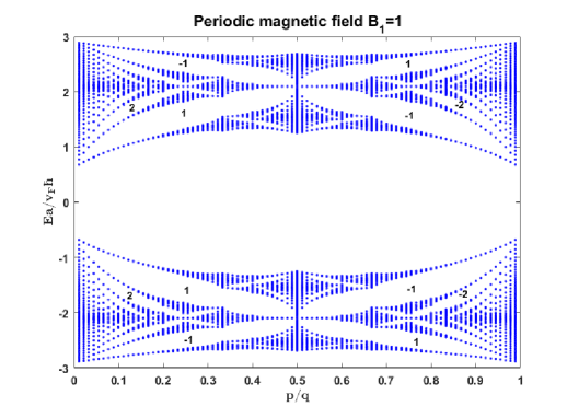
Figure 2: Dimensionless energy $\frac{Ea}{\hbar v_{F}}$ versus $\frac{p}{q}$ (Eq. 15) plot with Top: $B_{1}=0$ and Bottom: $B_{1}=1$. The values of p satisfy $1\leq p\leq q-1$, $a=0.25$ and $R^{s}=0.0825$ respectively.

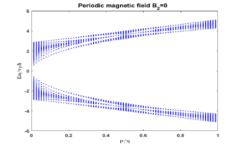
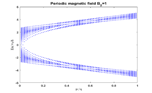
Figure 3: Dimensionless energy $\frac{Ea}{\hbar v_{F}}$ versus $p/q$ (Eq. 15) plot with Top: $B_{2}=0$ and, Bottom: $B_{2}=1$. Other parameters are same as Fig. 2

To simplify the problem further we set the condition $|\frac{ea^{2}}{\hbar c}(B_{u}+B_{p})|<<1$. For $B_{p}=0$, this condition translates into $a\ll l_{B_{u}},(l_{B_{u}}=\sqrt{\frac{\hbar c}{eB_{u}}})$, implying weak and slowly varying magnetic field Luttinger ; exact .

This type of condition is used in lattice gauge theory calculation Governale . Here using this we can write the eigenvalue equation ($\ref{eigval})$ in the form of discrete Schrödinger equation which takes the form of Hofstadter-Harper equation(details in suppli ).

$$\epsilon g(m,n) = e^{\frac{iea}{\hbar c}(A_{ux}+A_{px})}g(m+1,n)+e^{-\frac{iea}{\hbar c}(A_{ux}+A_{px})}g(m-1,n)+e^{\frac{iea}{\hbar c}(A_{uy}+A_{py})}g(m,n+1)$$ (15)

$$+ e^{-\frac{iea}{\hbar c}(A_{uy}+A_{py})}g(m,n-1)-(\frac{ea^{2}}{\hbar c}(B_{u}+B_{p})+4)g(m,n)$$

with $\epsilon=\frac{-E^{2}a^{2}}{v_{F}^{2}\hbar^{2}}$. It may be pointed out that in absolute value the magnetic field may still be substantially high and can provide substantial gap in the energy spectrum if the lattice separation is of the order of $\sim 100nm$ which is possible within current technology Bader .

The magnetic translation operator in Eq. $(\ref{magtran})$ forms magnetic translation group satisfying the algebra Brown

$$M_{\boldsymbol{R}_{1}}M_{\boldsymbol{R}_{2}} = \exp(\frac{2\pi i}{\phi_{0}}\phi)M_{\boldsymbol{R}_{2}}M_{\boldsymbol{R}_{1}}$$

$$M_{\boldsymbol{R}_{1}}M_{\boldsymbol{R}_{2}} = \exp(\frac{\pi i}{\phi_{0}}\phi)M_{\boldsymbol{R}_{1}+\boldsymbol{R}_{2}}$$ (16)

where $\phi=\boldsymbol{B}_{u}.(\boldsymbol{R}_{1}\times\boldsymbol{R}_{2})=\frac{p}{q}\phi_{0}$ is chosen as a rational number of flux quanta that passes through a unit cell. This defines the magnetic unit cell $\boldsymbol{R}^{\prime}=m(q)a\boldsymbol{\hat{x}}+na\boldsymbol{\hat{y}}$ such that $B_{u}qa^{2}=p$, an integer. This gives

$$B_{2}=((p/q)\phi_{0}-B_{1}\pi Rs^{2})/(a^{2}-\pi Rs^{2})$$ (17)

The corresponding Magnetic Brillouin zone (MBZ) is defined as $0\leq k_{x}\leq\frac{2\pi}{qa}$ and $0\leq k_{y}\leq\frac{2\pi}{a}$. If the redefined magnetic lattice has $N_{q}$ points along the $x$-axis and $N_{y}$ points along the $y$-axis then by construction $N_{q}q=2N_{max}+1=N_{y}$. The two ends of the lattice along $x$-axis and $y$-axis are connected by $\boldsymbol{R}_{x}=qN_{q}a\boldsymbol{\hat{x}}$ and $\boldsymbol{R}_{y}=N_{y}a\boldsymbol{\hat{y}}$ respectively. To solve the eigenvalue problem one can use condition along $x$ and $y$ axes as $M_{\boldsymbol{R}_{x}}\psi_{\boldsymbol{k}}^{a}(x,y))=\psi_{\boldsymbol{k}}^{a}(x,y)$ and $M_{\boldsymbol{R}_{y}}\psi_{\boldsymbol{k}}^{a}(x,y))=\psi_{\boldsymbol{k}}^{a}(x,y)$ where $\psi_{\boldsymbol{k}}^{a}(x,y))$ are the eigenfunctions of $H_{G}$. It can be checked Brown ; Munoz that if the number of fluxes through each unit cell is a rational number $\frac{p}{q}$, such boundary condition can be satisfied.

With the relation $(\ref{constraint1})$ and the mentioned boundary conditions we numerically solve the Eq. $(\ref{finalharper})$. The results are plotted in Fig. 2 and Fig. 3. In Fig. 2 (Top) and (Bottom) keeping $B_{1}=B_{u}+B_{p}$ fixed we plot the dimensionless energy $\pm\sqrt{-\epsilon}$ for the particle-hole spectrum Kohmoto2 as a function of $\frac{p}{q}$ for two different values of $B_{1}$. The increase in the gap between the particle and hole spectrum with increasing $B_{1}$ is clearly visible. The Fig. 3 on the other hand plots the same energy spectrum, but keeping $B_{2}$ fixed, for two representative values of $B_{2}$. For each value of $B_{2}$, in accordance with Eq. $(\ref{constraint1})$, $B_{1}$ varies with $\frac{p}{q}$ as we move along the horizontal axis. This causes variable gap between the particle and hole spectrum as $\frac{p}{q}$ changes. After discussing the spectrum of the hamiltonian in Eq. $(\ref{direq})$, we shall now evaluate the Hall conductance of the system and connect it with the spectrum.

The eigenfunctions of the hamiltonian (10) can also be written in the Bloch form as

$$\begin{bmatrix}\psi^{a}_{k_{x},k_{y}}\\ \psi^{b}_{k_{x},k_{y}}\end{bmatrix}=e^{i\boldsymbol{k}.\boldsymbol{r}}\begin{bmatrix}u^{a}_{k_{x},k_{y}}\\ u^{b}_{k_{x},k_{y}}\end{bmatrix}$$ (18)

We define $u^{\prime}_{k_{x},k_{y}}=\begin{bmatrix}u^{a}_{k_{x},k_{y}}\\ u^{b}_{k_{x},k_{y}}\end{bmatrix}.$ Since $B_{u}\neq 0$, the commutation relation (16) implies that $u^{a,b}_{k_{x},k_{y}}$ must have zeros inside a magnetic unit cell and have the structure $u^{a,b}_{k_{x},k_{y}}=|u^{a,b}_{k_{x},k_{y}}(x,y)|\exp(i\theta^{a,b}_{k_{x},k_{y}}(x,y))$ Kohmoto . These functions can be found by solving the Schrödinger Eq. $\hat{H}(k_{x},k_{y})u^{\prime n_{b}}_{k_{x},k_{y}}=E^{n_{b}}u^{\prime n_{b}}_{k_{x},k_{y}}$, where $n_{b}$ is the band index. Following TKNN Thouless1 the Hall conductance calculated through Kubo formula in the linear response regime for a completely filled band (the band index is omitted due to single band) can therefore be obtained as

$$\sigma_{xy}=\frac{e^{2}}{h}\frac{1}{2\pi i}\int d^{2}k[\boldsymbol{\nabla_{k}}\times\boldsymbol{\hat{A}}(k_{x},k_{y})]_{3}$$ (19)

where the integration is over the MBZ and

$$\boldsymbol{\hat{A}}(k_{x},k_{y})=\int d^{2}ru^{\prime*}_{k_{x},k_{y}}\boldsymbol{\nabla_{k}}u^{\prime}_{k_{x},k_{y}}$$ (20)

is the Berry connection defined over such MBZ. Since the two points $k_{x}=0$ and $k_{x}=\frac{2\pi}{qa}$ (or $k_{y}=0$ and $k_{y}=\frac{2\pi}{a}$) are equivalent, the MBZ has topology of a torus. The phase of the wave-function cannot be uniquely determined in the MBZ because of the existence of zeros of such wave function. This leads to finite value of the above integral and quantization of the Hall conductivity in this case giving

$$\sigma_{xy}=\frac{2e^{2}}{h}\sigma_{H}$$ (21)

where $\sigma_{H}$ is an integer. Here the factor 2 is coming due to sub-lattice degrees of freedom in single layer graphene. Thus if the Fermi energy lies in one of the gaps of the spectrum, the Hall conductivity is quantized in terms of an integer Thouless1 relevant to the filled band lying below the Fermi energy. Perturbations like disorder, interactions or effect of the higher order terms neglected in (15) can negate the above result only if the gap closes. Details of the calculation closely follow Kohmoto and are summarized in suppli .

To relate the integers in Eq. (21) with spectrum plotted in Fig. 2, we note that integration of the Berry connection $\boldsymbol{\hat{A}}(k_{x},k_{y})$ gives the geometric phase change of the functions $u^{\prime}_{k_{x},k_{y}}$ over the MBZ. Following Dana ; Wilkinson it is possible to show that the corresponding magnetic Bloch functions satisfy the boundary condition suppli

$$\psi_{k_{x}+\frac{b_{1}}{q},k_{y}}=\psi_{k_{x},k_{y}},~{}\psi_{k_{x},k_{y}+b_{2}}=e^{i\sigma_{H}k_{x}qa}\psi_{k_{x},k_{y}}$$ (22)

where $\boldsymbol{b}_{1}=\frac{2\pi}{a}\boldsymbol{\hat{x}}$ and $\boldsymbol{b}_{2}=\frac{2\pi}{a}\boldsymbol{\hat{y}}$ are the reciprocal lattice vectors. This condition must be consistent with the group properties defined in Eqs. (16) of the magnetic translation operator, given in Eq. (11), leading to

$$M_{a\boldsymbol{\hat{y}}}M_{a\boldsymbol{\hat{x}}}\psi_{\boldsymbol{k}}=e^{i(\boldsymbol{k}+\frac{p}{q}\boldsymbol{b}_{2}).a\boldsymbol{\hat{y}}}M_{a\boldsymbol{\hat{x}}}\psi_{\boldsymbol{k}}$$ (23)

where $M(a\boldsymbol{\hat{x}})\psi_{\boldsymbol{k}}$ depicts eigenfunction of $M(a\boldsymbol{\hat{y}})$ with eigenvalue $e^{i(\boldsymbol{k}+\frac{p}{q}\boldsymbol{b}_{2}).a\boldsymbol{\hat{y}}}$ . In the same way $M_{a\boldsymbol{\hat{x}}}\psi_{\boldsymbol{k}}$, ….$M_{(q-1)a\boldsymbol{\hat{x}}}\psi_{\boldsymbol{k}}$ all have different eigenvalue for $M_{a\boldsymbol{\hat{y}}}$, but same eigenvalue for the Hamiltonian. This leads to a $q$ fold degeneracy for each energy eigenvalue. The algebraic relation that connects the boundary condition in Eq. (22) with the relation (23), connects $\frac{p}{q}$ to the integer $\sigma_{H}$ through the famous Diaphantine Equation

$$\mu q+\sigma_{H}p=1$$ (24)

This equation is equivalent to the equation given by TKNN Thouless1 , for square lattice systems to calculate the Chern numbers associated with $\sigma_{H}$ for $r$th gap in a Landau level as $r=s_{r}q+t_{r}p$. Under the constraint $|t_{r}|\leq q/2$ this yields a unique solution $(s_{r},t_{r})$. Here $\sigma_{H}=t_{r}-t_{r-1}$ and $\mu=s_{r}-s_{r-1}$ Avron . In our system with square lattice magnetic modulation using the same method we calculate $t_{r}$ for few such swaths in Fig. 2.

To summarise we predict topological quantization of Hall conductivity for massless dirac fermions in monolayer graphene under generic two dimensional periodic magnetic modulation. The results can be extended to a non-relativistic 2DEG. Similar topological quantization in non bravais type of magnetic modulation in hexagonal lattice Rammal , effect of additional periodic electrostatic potential and (in)commensuration between two types of periodicities Hofstadter ; Gerhardts ; Gumbs , bulk and edge correspondence in such systemHalperin ; Muller will be some possible directions for further investigations. Periodic two dimensional magnetic modulation was already created for 2DEG in GaAs-AlGaAs heterojunctions using ferromagnetic dysprosium dots expt1 . Van der Waals heterostructure of monolayer graphene expt2 with layered magnetic materials such as Transition metal phosphorus trisulphide expt3 may also realize similar modulations.

We acknowledge helpful discussion and correspondence with S. Gupta, S. Shringarpure, M. Sharma and Itzhack Dana. MA is supported by a MHRD fellowship.

References

- (1) K. v. Klitzing, G. Dorda, and M. Pepper, Phys. Rev. Lett. 45, 494 (1980).
- (2) D. C. Tsui, H. L. Stormer, and A. C. Gossard, Phys. Rev. Lett. 48, 1559 (1982).
- (3) R. B. Laughlin, Phys. Rev. B 23, 5632 (1981).
- (4) B. I. Halperin, Phys. Rev. B 25, 2185 (1982).
- (5) K. S. Novoselov, A. K. Geim, S. V. Morozov, D. Jiang, M. I. Katnelson, I. V. Grigorieva, S. V. Dubonos, and A. A. Firsov, Nature(London) 438, 197 (2005).
- (6) Y. Zhang, Y-W Tan, H. L. Stormer and P. Kim, Nature(London) 438, 201(2005)
- (7) D. J. Thouless, M. Kohmoto, M. P. Nightingale, and M. den Nijs, Phys. Rev. Lett. 49, 405 (1982).
- (8) R. D. Hofstadter, Phys. Rev. B 14, 2239 (1976).
- (9) J. E. Avron, R. Seiler and B. Simon, Phys. Rev. Lett. 51, 51 (1983)
- (10) F. D. M. Haldane, Phys. Rev. Lett. 61, 2015 (1988).
- (11) C L. Cane and E. J. Mele, Phys. Rev. Lett. 95 226801 (2005).
- (12) B. A. Bernevig, T. A. Hughes and S. C. Zhang, Science, 314, 1757 (2006).
- (13) M. Z. Hasan and C. L. Kane, Rev. Mod. Phys. 82, 3045 (2010).
- (14) J. Zak, Phys. Rev. A: Gen. Phys. 134, 1607 (1964).
- (15) H. J. Fischbeck, Phys. Status Solidi 38, 11 (1970).
- (16) W. Florek, Act. Phys. Pol. A 92, 399-402 (1997).
- (17) A. D. Martino, L. Dell’Anna and R. Egger, Phys. Rev. Lett. 98, 066802 (2007).
- (18) A Matulis, F. M. Peeters and P. Vasilopoulos, Phys. Rev. Lett. 72, 1518 (1994).
- (19) M. C. Chang and Q. Niu, Phys. Rev. B 50, 10843 (1994).
- (20) G. -Y. Oh, Phys. Rev. B 60, 1939 (1999).
- (21) A. Krakovsky, Phys. Rev. B 53, 8469 (1996).
- (22) A. Nogaret, J. Phys. Cond. Matt. 22 253201 (2010).
- (23) N. Agrawal(Garg), S. Ghosh and M. Sharma, Int. Jour. of Mod. Phys. B, 27, 1341003 (2013).
- (24) P. D. Ye et al., Appl. Phys. Lett. 67, 1441 (1995).
- (25) S. D. Bader, Rev. Mod. Phys. 78, 1 (2006).
- (26) M. Taillefumier et al., Phys. Rev. B 78, 155330 (2008).
- (27) I. Snyman, Phys. Rev. B 80, 054303 (2009).
- (28) Supplementary information (description) shows various intermediate steps of certain derivations used in the main draft.
- (29) E. Brown, Solid State Physics (Ed. F. Seitz, D. Turnbull and H. Ehrenreich), 22, 313 (1969).
- (30) J. Zak, Phys. Rev. 139, A 1159 (1965)
- (31) Butterfly in the Quantum world, The story of most fascinating Quantum fractal, Indubala I. Satija (Morgan and Claypool Publishers, 2016), p. 10-3.
- (32) J. M. Luttinger, Phys. Rev. 84, 814 (1951).
- (33) G. H. Wannier and D. R. Fredkin, Phys. Rev. 125, 1910 (1962).
- (34) S. Janecek, M. Aichinger and E. R. Hernandez, Phys. Rev. B 87, 235429 (2013).
- (35) M. Governale and C. Ungarelli, Phys. Rev. B 58, 7816 (1998).
- (36) E. Brown, Phys. Rev. 133, A1038 (1964).
- (37) E Muoz, Z. Barticevic and M. Pacheco, Phys. Rev. B 71, 165301(2005).
- (38) Y. Hasegawa and M. Kohmoto, Phys. Rev. B 74, 155415 (2006).
- (39) Mahito Kohmoto, Annals of Physics 160, 343-354 (1984).
- (40) I. Dana, Y. Avron and J. Zak, J. Phys. C: Solid State Phys. 18, L679-L683 (1985).
- (41) M. Wilkinson, J. Phys.: Cond. Mat. 10, 7407-7427 (1998).
- (42) J. E. Avron, O. Kenneth, and G. Yehoshua, J. Phys. A: Math. Thoer. 47, 185202 (2014).
- (43) R. Rammal, J. Physique 46, 1345 (1985).
- (44) R. R. Gerhardts, D. Pfannkuche and V. Gudmundsson, Phys. Rev. B 53, 9591 (1996)
- (45) G. Gumbs, D. Miessein, and D. Huang, Phys. Rev. B 52, 14755 (1995).
- (46) J. E. Müller, Phys. Rev. Lett. 68, 385 (1992)
- (47) A. K. Geim and I. V. Grigorieva, Nature 499, 419 (2013).
- (48) J. G. Park, Jour Phys. Cond. Matt. 28, 301001 (2016).