Esthetic Numbers and Lifting Restrictions on the Analysis of Summatory Functions of Regular Sequences

Abstract.

When asymptotically analysing the summatory function of a $q$-regular sequence in the sense of Allouche and Shallit, the eigenvalues of the sum of matrices of the linear representation of the sequence determine the “shape” (in particular the growth) of the asymptotic formula. Existing general results for determining the precise behavior (including the Fourier coefficients of the appearing fluctuations) have previously been restricted by a technical condition on these eigenvalues.

The aim of this work is to lift these restrictions by providing an insightful proof based on generating functions for the main pseudo Tauberian theorem for all cases simultaneously. (This theorem is the key ingredient for overcoming convergence problems in Mellin–Perron summation in the asymptotic analysis.)

One example is discussed in more detail: A precise asymptotic formula for the amount of esthetic numbers in the first $N$ natural numbers is presented. Prior to this only the asymptotic amount of these numbers with a given digit-length was known.

1. Introduction

This extended abstract studies the asymptotic behaviour of summatory functions of $q$-regular sequences. We start with a definition of $q$-regular sequences.

1.1. $q$-Regular Sequences

An introduction and formal definition of $q$-regular sequences (via the so-called $q$-kernel) is given by Allouche and Shallit [1] and [2, Chapter 16]. We settle here for an equivalent formulation which is the most useful for our considerations.

Let $q\geq 2$ be a fixed integer and $(x(n))_{n\geq 0}$ be a sequence. Then $(x(n))_{n\geq 0}$ is $q$-regular if and only if there exists a vector valued sequence $(v(n))_{n\geq 0}$ whose first component coincides with $(x(n))_{n\geq 0}$ and there exist square matrices $A_{0}$, …, $A_{q-1}\in\mathbb{C}^{d\times d}$ such that

$$v(qn+r)=A_{r}v(n)\qquad\text{for $0\leq r<q$, $n\geq 0$;}$$ (1.1)

see Allouche and Shallit [1, Theorem 2.2]. This is called a $q$-linear representation of $x(n)$.

We note that a linear representation (1.1) immediately leads to an explicit expression for $x(n)$ by induction: Let $r_{\ell-1}\ldots r_{0}$ be the $q$-ary digit expansion of $n$. Then

$$x(n)=e_{1}A_{r_{0}}\dotsm A_{r_{\ell-1}}v(0)$$

where $e_{1}=\begin{pmatrix}1&0&\dotsc&0\end{pmatrix}$.

Regular sequences are related to divide-and-conquer algorithms, therefore they have been intensively investigated in the literature in many particular cases; see, for example, [5], [6], [7], [8] [10], [11], [12], [13] and [14] for a more detailed overview. The best-known example for a $2$-regular function is the binary sum-of-digits function.

1.2. Summatory Functions

Of particular interest is the analysis of the summatory function (i.e., the sequence of partial sums) of a regular sequence, not least because of its relation to the expectation of a random element of the sequence (with respect to uniform distribution on the nonnegative integers smaller than a certain $N$). In [12], Prodinger and the two authors of this extended abstract provide a theorem decomposing the summatory function into periodic fluctuations multiplied by some scaling functions; the Fourier coefficients of these periodic fluctuations are provided as well. Although this result is quite general, the proof in [12] imposes a restriction on the asymptotic growth. One major aim of this work is to lift this restriction by completely getting rid of the corresponding technical condition. We formulate the full main theorem in Section 3 and the theorem stating the underlying pseudo-Tauberian argument in Section 4.

1.3. The Proof

The proof of the extended pseudo-Tauberian theorem contained in this extended abstract not only covers the previously excluded cases, but also works for the existing theorem in [12]. In particular the proof of the main result does not need a case distinction, but the contained proof supersedes the existing one. (Besides, it also is much shorter.) This is reached by changing the perspective to a more general point of view; we use a generating functions approach. Beside proving the theorem, this also gives additional insights. For example, the cancellations in the proof in [12] seem to be a kind of magic at that point, but with the new approach, it is now clear and no surprise anymore that they have to appear.

1.4. Esthetic Numbers

A further main contribution of this extended abstract is the precise asymptotic analysis of $q$-esthetic numbers, see De Koninck and Doyon [3]. These are numbers whose $q$-ary digit expansion satisfies the condition that neighboring digits differ by exactly one. The sequence of such numbers turns out to be $q$-automatic, thus are $q$-regular and can also be seen as an output sum of a transducer; see the first author’s joint work with Kropf and Prodinger [13]. However, the asymptotics obtained by using the main result of [13]—in fact, this result is recovered as a corollary of the main result of [12]—is degenerated in the sense that the provided main term and second order term both equal zero. On the other hand, using a more direct approach via our main theorem brings up the actual main term and the fluctuation in this main term. The full theorem is formulated in Section 2. Prior to this precise analysis, the authors of [3] only performed an analysis of esthetic numbers by digit-length (and not by the number itself).

The approach used in the analysis of $q$-esthetic numbers can easily be adapted to numbers defined by other conditions on the word of digits of their $q$-ary expansion.

1.5. Dependence on Residue Classes

The analysis of $q$-esthetic numbers also brings another aspect into the light of day, namely a quite interesting dependence of the behaviour with respect to $q$ on different moduli:

• The dimensions in the matrix approach of [3] need to be increased for certain residue classes of $q$ modulo $4$ in order to get a formulation as a $q$-automatic and $q$-regular sequence, respectively.

• The main result in [3] already depends on the parity of $q$ (i.e., on $q$ modulo $2$). This reflects our Theorem A by having $2$-periodic fluctuations (in contrast to $1$-periodic fluctuations in the main Theorem B).

• Surprisingly, the error term in the resulting formula of Theorem A depends on the residue class of $q$ modulo $3$. This is due to the appearance of an eigenvalue $1$ in certain cases.

• As an interesting side-note: In the same (up to this point not specified; see below) spectrum, the algebraic multiplicity of the eigenvalue $0$ changes again only modulo $2$.

The spectrum above consists of the eigenvalues of the sum of matrices of the $q$-linear representation of the sequence.

1.6. Symmetrically Arranged Eigenvalues

The second of the four bullet points above comes from a particular configuration in the spectrum. Whenever eigenvalues are arranged as vertices of a regular polygon, then their influence can be collected; this results in periodic fluctuations with larger period than $1$. We elaborate on the influence of such eigenvalues in Section 5. This is then used in the particular case of esthetic numbers, but might also be used in conjunction with the output sum of transducers; to be precise, for obtaining the second order term in the main result of [13].

2. Esthetic Numbers

Let again be $q\geq 2$ a fixed integer. We call a nonnegative integer $n$ a $q$-esthetic number (or simply an esthetic number) if its $q$-ary digit expansion $r_{\ell-1}\dots r_{0}$ satisfies $\lvert r_{j}-r_{j-1}\rvert=1$ for all $j\in\{1,\dots,\ell-1\}$; see De Koninck and Doyon [3].

In [3] the authors count $q$-esthetic numbers with a given length of their $q$-ary digit expansion. They provide an exact as well as an asymptotic formula for these counts. We aim for a more precise analysis and head for an asymptotic description of the amount of $q$-esthetic numbers up the an arbitrary value $N$ (in contrast to only powers of $q$ in [3]).

2.1. A $q$-Linear Representation

Figure 2.1. Automaton $\mathcal{A}$ recognizing esthetic numbers.

The language consisting of the $q$-ary digit expansions (seen as words of digits) which are $q$-esthetic is a regular language, because it is recognized by the automaton $\mathcal{A}$ in Figure 2.1. Therefore, the indicator sequence of this language, i.e., the $n$th entry is $1$ if $n$ is $q$-esthetic and $0$ otherwise is a $q$-automatic sequence and therefore also $q$-regular. Let us name this sequence $x(n)$.

Let $A_{0}$, …, $A_{q-1}$ be the transition matrices of the automaton $\mathcal{A}$, i.e., $A_{r}$ is the adjacency matrix of the directed graph induced by a transition with digit $r$. To make this more explicit, we have the following $(q+1)$-dimensional square matrices: Each row and column corresponds to the states $0$, $1$, …, $q-1$, $\mathcal{I}$. In matrix $A_{r}$, the only nonzero entries are in column $r\in\{0,1,\dots,q-1\}$, namely $1$ in the rows $r-1$ and $r+1$ (if available) and in row $\mathcal{I}$ as there are transitions from these states to state $r$ in the automaton $\mathcal{A}$.

Let us make this more concrete by considering $q=4$. We obtain the matrices

$$A_{0} =\scalebox{0.8}{$\begin{pmatrix}0&0&0&0&0\\ 1&0&0&0&0\\ 0&0&0&0&0\\ 0&0&0&0&0\\ 1&0&0&0&0\end{pmatrix}$}, A_{1} =\scalebox{0.8}{$\begin{pmatrix}0&1&0&0&0\\ 0&0&0&0&0\\ 0&1&0&0&0\\ 0&0&0&0&0\\ 0&1&0&0&0\end{pmatrix}$}, A_{2} =\scalebox{0.8}{$\begin{pmatrix}0&0&0&0&0\\ 0&0&1&0&0\\ 0&0&0&0&0\\ 0&0&1&0&0\\ 0&0&1&0&0\end{pmatrix}$}, A_{3} =\scalebox{0.8}{$\begin{pmatrix}0&0&0&0&0\\ 0&0&0&0&0\\ 0&0&0&1&0\\ 0&0&0&0&0\\ 0&0&0&1&0\end{pmatrix}$}.$$

We are almost at a $q$-linear representation of our sequence; we still need vectors on both sides of the matrix products. We have

$$x(n)=e_{q+1}\,A_{r_{0}}\cdots A_{r_{\ell-1}}v(0)$$

for $r_{\ell-1}\dots r_{0}$ being the $q$-ary expansion of $n$ and chosen vectors $e_{q+1}=\begin{pmatrix}0&\dotsc&0&1\end{pmatrix}$ and $v(0)=\begin{pmatrix}0&1&\dotsc&1\end{pmatrix}^{\top}$. Strictly speaking, this is not yet a regular sequence: in the case of regular sequences, we always have that $A_{0}v(0)=v(0)$ which is not the case here. This does not matter in this case: the difference leads to an additional constant in the asymptotic analysis which is absorbed by the error term anyway.

To see that the above holds, we have two different interpretations: The first is that the row vector $w(n)=e_{q+1}\,A_{r_{0}}\cdots A_{r_{\ell-1}}$ is the unit vector corresponding to the most significant digit of the $q$-ary expansion of $n$ or, in view of the automaton $\mathcal{A}$, corresponding to the final state. Note that we read the digit expansion from the least significant digit to the most significant one (although it would be possible the other way round as well). We have $w(0)=e_{q+1}$ which corresponds to the empty word and being in the initial state $\mathcal{I}$ in the automaton. The vector $v(0)$ corresponds to the fact that all states of $\mathcal{A}$ except $0$ are accepting.

The other interpretation is: The $r$th component of the column vector $v(n)=A_{r_{0}}\cdots A_{r_{\ell-1}}v(0)$ has the following two meanings:

• In the automaton $\mathcal{A}$, we start in state $r$ and then read the digit expansion of $n$. The $r$th component is then the indicator function whether we remain esthetic, i.e., end in an accepting state.

• To a word ending with $r$ we append the digit expansion of $n$. The $r$th component is then the indicator function whether the result is an esthetic word.

At first glance, our problem here seems to be a special case of the transducers studied in [13]. However, the automaton $\mathcal{A}$ is not complete. Adding a sink to have a formally complete automaton, however, adds an eigenvalue $q$ and thus a much larger dominant asymptotic term, which would then be multiplied by $0$. Therefore, the results of [13] do not apply to this case here.

2.2. Full Asymptotics

We now formulate our main result for the amount of esthetic numbers smaller than a given integer $N$. We abbreviate this amount by $X(N)=\sum_{0\leq n<N}x(n)$ and have the following theorem.

Theorem A.

The number $X(N)$ of $q$-esthetic numbers smaller than $N$ is

$$X(N)=\sum_{j\in\{1,2,\dots,\lceil\frac{q-2}{3}\rceil\}}N^{\log_{q}(2\cos(j\pi/(q+1)))}\Phi_{qj}(2\{\log_{q^{2}}N\})+\mathop{{O}{}}\big{(}(\log N)^{[q\equiv-1{\@displayfalse\pmod{3}}]}\big{)}$$ (2.1)

with $2$-periodic continuous functions $\Phi_{qj}$. Moreover, we can effectively compute the Fourier coefficients of each $\Phi_{qj}$. If $q$ is even, then the functions $\Phi_{qj}$ are actually $1$-periodic.

If $q=2$, then the theorem results in $X(N)=\mathop{{O}{}}(\log N)$. However, for each length, the only word of digits satisfying the esthetic number condition has alternating digits $0$ and $1$, starting with $1$ at its most significant digit. The corresponding numbers $n$ are the sequence A000975 (“Lichtenberg sequence”) in The On-Line Encyclopedia of Integer Sequences [15].

Back to a general $q$: For the asymptotics, the main quantities influencing the growth will turn out to be the eigenvalues of the matrix $C=A_{0}+\dots+A_{q-1}$. Continuing our example $q=4$ above, this matrix is

$$C=A_{0}+A_{1}+A_{2}+A_{3}=\scalebox{0.8}{$\begin{pmatrix}0&1&0&0&0\\ 1&0&1&0&0\\ 0&1&0&1&0\\ 0&0&1&0&0\\ 1&1&1&1&0\end{pmatrix}$},$$

and its eigenvalues are $\pm 2\cos(\frac{\pi}{5})=\pm\frac{1}{2}\bigl{(}\sqrt{5}+1\bigr{)}=\pm 1.618\dots$, $\pm 2\cos(\frac{2\pi}{5})=\pm\frac{1}{2}\bigl{(}\sqrt{5}-1\bigr{)}=\pm 0.618\dots$ and $0$, all with algebraic and geometric multiplicity $1$. Therefore it turns out that the growth of the main term is $N^{\log_{4}(\sqrt{5}+1)-\frac{1}{2}}=N^{0.347\dots}$, see Figure 2.2

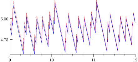
Figure 2.2. Fluctuation in the main term of the asymptotic expansion of $X(N)$ for $q=4$. The figure shows $\mathop{{#1}{}}(u)$ (red) approximated by its trigonometric polynomial of degree $1999$ as well as $X(4^{u})/N^{u(\log_{4}(\sqrt{5}+1)-\frac{1}{2})}$ (blue).

The proof of Theorem A can be found in Appendix B.

3. Asymptotics of Summatory Functions

3.1. Main Result on the Asymptotics

We are interested in the asymptotic behaviour of the summatory function $X(N)=\sum_{0\leq n<N}x(n)$.

We choose any vector norm $\lVert\,\cdot\,\rVert$ on $\mathbb{C}^{d}$ and its induced matrix norm. We set $C\coloneqq\sum_{r=0}^{q-1}A_{r}$. We choose $R>0$ such that $\lVert A_{r_{1}}\dotsm A_{r_{\ell}}\rVert=\mathop{{O}{}}(R^{\ell})$ holds for all $\ell\geq 0$ and $0\leq r_{1},\dotsc,r_{\ell}<q$. In other words, $R$ is an upper bound for the joint spectral radius of $A_{1}$, …, $A_{q-1}$. The spectrum of $C$, i.e., the set of eigenvalues of $C$, is denoted by $\sigma(C)$. For $\lambda\in\mathbb{C}$, let $m(\lambda)$ denote the size of the largest Jordan block of $C$ associated with $\lambda$; in particular, $m(\lambda)=0$ if $\lambda\notin\sigma(C)$. Finally, we consider the Dirichlet series

$$\mathcal{X}(s)=\sum_{n\geq 1}n^{-s}x(n),\qquad\mathcal{V}(s)=\sum_{n\geq 1}n^{-s}v(n)$$

where $v(n)$ is the vector valued sequence defined in (1.1). Of course, $\mathcal{X}(s)$ is the first component of $\mathcal{V}(s)$. The principal value of the complex logarithm is denoted by $\log$. The fractional part of a real number $z$ is denoted by $\{z\}\coloneqq z-\lfloor z\rfloor$.

Theorem B.

With the notations above, we have

$$X(N)=\sum_{\begin{subarray}{c}\lambda\in\sigma(C)\\ \lvert\lambda\rvert>R\end{subarray}}N^{\log_{q}\lambda}\sum_{0\leq k<m(\lambda)}(\log_{q}N)^{k}\Phi_{\lambda k}(\{\log_{q}N\})\\ +\mathop{{O}{}}\big{(}N^{\log_{q}R}(\log N)^{\max\{m(\lambda)\colon\mathopen{}\lvert\lambda\rvert=R\}}\big{)}$$ (3.1)

for suitable $1$-periodic continuous functions $\Phi_{\lambda k}$. If there are no eigenvalues $\lambda\in\sigma(C)$ with $\lvert\lambda\rvert\leq R$, the $O$-term can be omitted.

For $\lvert\lambda\rvert>R$ and $0\leq k<m(\lambda)$, the function $\Phi_{\lambda k}$ is Hölder continuous with any exponent smaller than $\log_{q}(\lvert\lambda\rvert/R)$.

The Dirichlet series $\mathcal{V}(s)$ converges absolutely and uniformly on compact subsets of the half plane $\Re s>\log_{q}R+1$ and can be continued to a meromorphic function on the half plane $\Re s>\log_{q}R$. It satisfies the functional equation

$$(I-q^{-s}C)\mathcal{V}(s)=\sum_{n=1}^{q-1}n^{-s}v(n)+q^{-s}\sum_{r=0}^{q-1}A_{r}\sum_{k\geq 1}\binom{-s}{k}\Bigl{(}\frac{r}{q}\Bigr{)}^{k}\mathcal{V}(s+k)$$ (3.2)

for $\Re s>\log_{q}R$. The right side converges absolutely and uniformly on compact subsets of $\Re s>\log_{q}R$. In particular, $\mathcal{V}(s)$ can only have poles where $q^{s}\in\sigma(C)$.

For $\lambda\in\sigma(C)$ with $\lvert\lambda\rvert>R$, the Fourier series

$$\Phi_{\lambda k}(u)=\sum_{\ell\in\mathbb{Z}}\varphi_{\lambda k\ell}\exp(2\ell\pi iu)$$

converges pointwise for $u\in\mathbb{R}$ where

$$\varphi_{\lambda k\ell}=\frac{(\log q)^{k}}{k!}\operatorname{Res}\bigg{(}\frac{\bigl{(}x(0)+\mathcal{X}(s)\bigr{)}\bigl{(}s-\log_{q}\lambda-\frac{2\ell\pi i}{\log q}\bigr{)}^{k}}{s},s=\log_{q}\lambda+\frac{2\ell\pi i}{\log q}\bigg{)}$$ (3.3)

for $\ell\in\mathbb{Z}$, $0\leq k<m(\lambda)$.

The above theorem is almost the formulation found in [12], but with the important difference that the technical condition $\lvert\lambda\rvert>\max\{R,1/q\}$ is replaced with the condition $\lvert\lambda\rvert>R$. The latter condition is inherent in the problem: single summands $x(n)$ might be as large as $n^{\log_{q}R}$ and must therefore be absorbed by the error term in any smooth asymptotic formula for the summatory function.

Sketch of Proof of Theorem B.

Use the proof of the corresponding theorem in [12], but replace the pseudo-Tauberian argument by Theorem C. ∎

3.2. Fourier Coefficients & Mellin–Perron Summation

We give a heuristic and non-rigorous argument explaining why the formula (3.3) for the Fourier coefficients is expected; see also [4].

By the Mellin–Perron summation formula of order $0$ (see, for example, [9, Theorem 2.1]), we have

$$\sum_{1\leq n<N}x(n)+\frac{x(N)}{2}=\frac{1}{2\pi i}\int_{\max\{\log_{q}R+2,1\}-i\infty}^{\max\{\log_{q}R+2,1\}+i\infty}\mathcal{X}(s)\frac{N^{s}\,\mathrm{d}s}{s}.$$

Shifting the line of integration to the left and collecting the residues at the location of the poles of $\mathcal{X}(s)$ claimed in Theorem B yields the Fourier series expansion. However, we have no analytic justification that this is allowed, so we need to work around this issue by reducing the problem to higher order Mellin–Perron summation; details are to be found in [12]. One key ingredient to make tracks back to our original summation problem is a pseudo-Tauberian theorem; see below.

4. Pseudo-Tauberian Theorem

In this section, we generalise a pseudo-Tauberian argument by Flajolet, Grabner, Kirschenhofer, Prodinger and Tichy [9, Proposition 6.4]. In contrast to their version, we allow for an additional logarithmic factor, have weaker growth conditions on the Dirichlet series and quantify the error. We also extend the result to all complex $\kappa$.

Theorem C.

Let $\kappa\in\mathbb{C}$ and $q>1$ be a real number, $m$ be a positive integer, $\Phi_{0}$, …, $\Phi_{m-1}$ be $1$-periodic Hölder continuous functions with exponent $\alpha>0$, and $0<\beta<\alpha$. Then there exist continuously differentiable functions $\Psi_{-1}$, $\Psi_{0}$, …, $\Psi_{m-1}$, periodic with period $1$, and a constant $c$ such that

$$\sum_{1\leq n<N}n^{\kappa}\sum_{\begin{subarray}{c}j+k=m-1\\ 0\leq j<m\end{subarray}}\frac{(\log n)^{k}}{k!}\Phi_{j}(\log_{q}n)\\ =c+N^{\kappa+1}\sum_{\begin{subarray}{c}k+j=m-1\\ -1\leq j<m\end{subarray}}\frac{(\log N)^{k}}{k!}\Psi_{j}(\log_{q}N)+\mathop{{O}{}}\big{(}N^{\Re\kappa+1-\beta}\big{)}$$ (4.1)

for integers $N\to\infty$.

Denote the Fourier coefficients of $\Phi_{j}$ and $\Psi_{j}$ by $\varphi_{j\ell}\coloneqq\int_{0}^{1}\Phi_{j}(u)\exp(-2\ell\pi iu)\,\mathrm{d}u$ and $\psi_{j\ell}\coloneqq\int_{0}^{1}\Psi_{j}(u)\exp(-2\ell\pi iu)\,\mathrm{d}u$, respectively. Then the corresponding generating functions fulfil

$$\sum_{0\leq j<m}\varphi_{j\ell}Z^{j}=\Bigl{(}\kappa+1+\frac{2\ell\pi i}{\log q}+Z\Bigr{)}\sum_{-1\leq j<m}\psi_{j\ell}Z^{j}+\mathop{{O}{}}(Z^{m})$$ (4.2)

for $\ell\in\mathbb{Z}$ and $Z\to 0$.

If $q^{\kappa+1}\neq 1$, then $\Psi_{-1}$ vanishes.

Remark 4.1.

Note that the constant $c$ is absorbed by the error term if $\Re\kappa+1>\alpha$, in particular if $\Re\kappa>0$. Therefore, this constant does not occur in the article [9].

Remark 4.2.

The factor $\kappa+1+\frac{2\ell\pi i}{\log q}+Z$ in (4.2) will turn out to correspond exactly to the additional factor $s+1$ in the first order Mellin–Perron summation formula with the substitution $s=\kappa+\frac{2\ell\pi i}{\log q}+Z$ such that the local expansion around the pole in $s=\kappa+\frac{2\ell\pi i}{\log q}$ of the Dirichlet generating function is conveniently written as a Laurent series in $Z$.

Proof.

Notations. Without loss of generality, we assume that $q^{\Re\kappa+1}\neq q^{\alpha}$: otherwise, we slightly decrease $\alpha$ keeping the inequality $\beta<\alpha$ intact. We use the abbreviations $\Lambda\coloneqq\lfloor\log_{q}N\rfloor$, $\nu\coloneqq\{\log_{q}N\}$, i.e., $N=q^{\Lambda+\nu}$. We use the generating functions

$$\mathop{{#1}{}}(u,Z) \coloneqq\sum_{0\leq j<m}\Phi_{j}(u)Z^{j},$$

$$L(N,Z) \coloneqq\sum_{1\leq n<N}n^{\kappa+Z}\mathop{{#1}{}}(\log_{q}n,Z)=\sum_{1\leq n<N}n^{\kappa}\exp\big{(}(\log n)Z\big{)}\mathop{{#1}{}}(\log_{q}n,Z),$$

$$Q(Z) \coloneqq q^{\kappa+1+Z}$$

for $0\leq u\leq 1$ and $0<\lvert Z\rvert<2r$ where $r>0$ is chosen such that $r<(\alpha-\beta)/2$ and such that $Q(Z)\neq 1$ and $\lvert Q(Z)\rvert\neq q^{\alpha}$ for these $Z$. (The condition $Z\neq 0$ is only needed for the case $q^{1+\kappa}=1$.) We will stick to the above choice of $r$ and restrictions for $Z$ throughout the proof.

It is easily seen that the left-hand side of (4.1) equals $[Z^{m-1}]L(N,Z)$, where $[Z^{m-1}]$ denotes extraction of the coefficient of $Z^{m-1}$.

Approximation of the Sum by an Integral. Splitting the range of summation with respect to powers of $q$ yields

$$L(N,Z)=\phantom{+\;} \sum_{0\leq p<\Lambda}\sum_{q^{p}\leq n<q^{p+1}}n^{\kappa+Z}\mathop{{#1}{}}(\log_{q}n,Z)$$

$$+\; \sum_{q^{\Lambda}\leq n<q^{\Lambda+\nu}}n^{\kappa+Z}\mathop{{#1}{}}(\log_{q}n,Z).$$

We write $n=q^{p}x$ (or $n=q^{\Lambda}x$ for the second sum), use the periodicity of $\Phi$ in $u$ and get

$$L(N,Z)=\phantom{+\;} \sum_{0\leq p<\Lambda}Q(Z)^{p}\sum_{\begin{subarray}{c}x\in q^{-p}\mathbb{Z}\\ 1\leq x<q\end{subarray}}x^{\kappa+Z}\mathop{{#1}{}}(\log_{q}x,Z)\frac{1}{q^{p}}$$

$$+\; Q(Z)^{\Lambda}\sum_{\begin{subarray}{c}x\in q^{-\Lambda}\mathbb{Z}\\ 1\leq x<q^{\nu}\end{subarray}}x^{\kappa+Z}\mathop{{#1}{}}(\log_{q}x,Z)\frac{1}{q^{\Lambda}}.$$

The inner sums are Riemann sums converging to the corresponding integrals for $p\to\infty$. We set

$$I(u,Z)\coloneqq\int_{1}^{q^{u}}x^{\kappa+Z}\mathop{{#1}{}}(\log_{q}x,Z)\,\mathrm{d}x.$$

It will be convenient to change variables $x=q^{w}$ in $I(u,Z)$ to get

$$I(u,Z)=(\log q)\int_{0}^{u}Q(Z)^{w}\mathop{{#1}{}}(w,Z)\,\mathrm{d}w.$$ (4.3)

We define the error $\varepsilon_{p}(u,Z)$ by

$$\sum_{\begin{subarray}{c}x\in q^{-p}\mathbb{Z}\\ 1\leq x<q^{u}\end{subarray}}x^{\kappa+Z}\mathop{{#1}{}}(\log_{q}x,Z)\frac{1}{q^{p}}=I(u,Z)+\varepsilon_{p}(u,Z).$$

As the sum and the integral are both analytic in $Z$, their difference $\varepsilon_{p}(u,Z)$ is analytic in $Z$, too. We bound $\varepsilon_{p}(u,Z)$ by the difference of upper and lower Darboux sums (step size $q^{-p}$) corresponding to the integral $I(u,Z)$: On each interval of length $q^{-p}$, the maximum and minimum of a Hölder continuous function can differ by at most $\mathop{{O}{}}(q^{-\alpha p})$. As the integration interval as well as the range for $u$ and $Z$ are finite, this translates to the bound $\varepsilon_{p}(u,Z)=\mathop{{O}{}}(q^{-\alpha p})$ as $p\to\infty$ uniformly in $0\leq u\leq 1$ and $\lvert Z\rvert<2r$. This results in

$$L(N,Z)=I(1,Z)\sum_{0\leq p<\Lambda}Q(Z)^{p}+\sum_{0\leq p<\Lambda}Q(Z)^{p}\varepsilon_{p}(1,Z)+I(\nu,Z)\,Q(Z)^{\Lambda}+Q(Z)^{\Lambda}\varepsilon_{\Lambda}(\nu,Z).$$

If $\lvert Q(Z)\rvert/q^{\alpha}=q^{\Re\kappa+1+\Re Z-\alpha}<1$, i.e., $\Re\kappa+\Re Z<\alpha-1$, the second sum involving the integration error converges absolutely and uniformly in $Z$ for $\Lambda\to\infty$ to some analytic function $c^{\prime}(Z)$; therefore, we can replace the second sum by $c^{\prime}(Z)+\mathop{{O}{}}\big{(}q^{(\Re\kappa+1+2r-\alpha)\Lambda}\big{)}=c^{\prime}(Z)+\mathop{{O}{}}\big{(}N^{\Re\kappa+1+2r-\alpha}\big{)}$ in this case. If $\Re\kappa+\Re Z>\alpha-1$, then the second sum is $\mathop{{O}{}}\big{(}q^{(\Re\kappa+2r+1-\alpha)\Lambda}\big{)}=\mathop{{O}{}}\big{(}N^{\Re\kappa+1+2r-\alpha}\big{)}$. By our choice of $r$, the case $\Re\kappa+\Re Z=\alpha-1$ cannot occur. So in any case, we may write the second sum as $c^{\prime}(Z)+\mathop{{O}{}}\big{(}N^{\Re\kappa+1-\beta}\big{)}$ by our choice of $r$. The last summand involving $\varepsilon_{\Lambda}(\nu,Z)$ is absorbed by the error term of the second summand. Note that the error term is uniform in $Z$ and, by its construction, analytic in $Z$.

Thus we end up with

$$L(N,Z)=c^{\prime}(Z)+S(N,Z)+\mathop{{O}{}}\big{(}N^{\Re\kappa+1-\beta}\big{)}$$ (4.4)

where

$$S(N,Z)\coloneqq I(1,Z)\sum_{0\leq p<\Lambda}Q(Z)^{p}+I(\nu,Z)Q(Z)^{\Lambda}.$$ (4.5)

It remains to rewrite $S(N,Z)$ in the form required by (4.1). We emphasise that we will compute $S(N,Z)$ exactly, i.e., no more asymptotics for $N\to\infty$ will play any rôle.

Construction of $\Psi$. We rewrite (4.5) as

$$S(N,Z) =I(1,Z)\frac{1-\mathop{{#1}{}}(Z)^{\Lambda}}{1-\mathop{{#1}{}}(Z)}+I(\nu,Z)\mathop{{#1}{}}(Z)^{\Lambda}.$$

We replace $\Lambda$ by $\log_{q}N-\nu$ and use

$$\mathop{{#1}{}}(Z)^{\Lambda} =\mathop{{#1}{}}(Z)^{\log_{q}N}\mathop{{#1}{}}(Z)^{-\nu}=N^{\kappa+1+Z}\mathop{{#1}{}}(Z)^{-\nu}$$

to get

$$S(N,Z)=\frac{I(1,Z)}{1-\mathop{{#1}{}}(Z)}+N^{\kappa+1+Z}\Psi(\nu,Z)$$ (4.6)

with

$$\Psi(u,Z)\coloneqq\mathop{{#1}{}}(Z)^{-u}\Bigl{(}I(u,Z)-\frac{I(1,Z)}{1-\mathop{{#1}{}}(Z)}\Bigr{)}.$$ (4.7)

Periodic Extension of $\Psi$. It is obvious that $\mathop{{#1}{}}(u,Z)$ is continuously differentiable in $u\in[0,1]$. We have

$$\mathop{{#1}{}}(1,Z)=\frac{I(1,Z)}{\mathop{{#1}{}}(Z)}\Bigl{(}1-\frac{1}{1-\mathop{{#1}{}}(Z)}\Bigr{)}=-\frac{I(1,Z)}{1-\mathop{{#1}{}}(Z)}=\mathop{{#1}{}}(0,Z)$$

because $I(0,Z)=0$ by (4.3). The derivative of $\mathop{{#1}{}}(u,Z)$ with respect to $u$ is

$$\frac{\partial\mathop{{#1}{}}(u,Z)}{\partial u} =-\bigl{(}\log\mathop{{#1}{}}(Z)\bigr{)}\mathop{{#1}{}}(u,Z)+(\log q)\mathop{{#1}{}}(Z)^{-u}\mathop{{#1}{}}(Z)^{u}\mathop{{#1}{}}(u,Z)$$

$$=-\bigl{(}\log\mathop{{#1}{}}(Z)\bigr{)}\mathop{{#1}{}}(u,Z)+(\log q)\mathop{{#1}{}}(u,Z),$$

which implies that

$$\frac{\partial\mathop{{#1}{}}(u,Z)}{\partial u}\Bigr{|}_{u=1}=\frac{\partial\mathop{{#1}{}}(u,Z)}{\partial u}\Bigr{|}_{u=0}.$$

We can therefore extend $\mathop{{#1}{}}(u,Z)$ to a $1$-periodic continuously differentiable function in $u$ on $\mathbb{R}$.

Fourier Coefficients of $\Psi$. By using equations (4.7) and (4.3), $Q(Z)=q^{\kappa+1+Z}$, and $\exp(-2\ell\pi iu)=q^{-\chi_{\ell}u}$ with $\chi_{\ell}=\frac{2\pi i\ell}{\log q}$, we now express the Fourier coefficients of $\mathop{{#1}{}}(u,Z)$ in terms of those of $\mathop{{#1}{}}(u,Z)$ by

$$\int_{0}^{1}\mathop{{#1}{}}(u,Z)\exp(-2\ell\pi iu)\,\mathrm{d}u\\ \begin{aligned} &=(\log q)\int_{0\leq w\leq u\leq 1}\mathop{{#1}{}}(Z)^{w-u}\mathop{{#1}{}}(w,Z)q^{-\chi_{\ell}u}\,\mathrm{d}w\,\mathrm{d}u\\ &\phantom{=}\;-\frac{I(1,Z)}{1-\mathop{{#1}{}}(Z)}\int_{0}^{1}q^{-(\kappa+1+Z+\chi_{\ell})u}\,\mathrm{d}u\\ &=(\log q)\int_{0\leq w\leq 1}\mathop{{#1}{}}(Z)^{w}\mathop{{#1}{}}(w,Z)\int_{w\leq u\leq 1}q^{-(\kappa+1+Z+\chi_{\ell})u}\,\mathrm{d}u\,\mathrm{d}w\\ &\phantom{=}\;-\frac{I(1,Z)}{(1-\mathop{{#1}{}}(Z))(\log q)(\kappa+1+Z+\chi_{\ell})}\Bigl{(}1-\frac{1}{\mathop{{#1}{}}(Z)}\Bigr{)}\\ &=\frac{1}{\kappa+1+Z+\chi_{\ell}}\int_{0}^{1}\mathop{{#1}{}}(Z)^{w}\mathop{{#1}{}}(w,Z)\Bigl{(}q^{-(\kappa+1+Z+\chi_{\ell})w}-\frac{1}{\mathop{{#1}{}}(Z)}\Bigr{)}\,\mathrm{d}w\\ &\phantom{=}\;+\frac{I(1,Z)}{\mathop{{#1}{}}(Z)(\log q)(\kappa+1+Z+\chi_{\ell})}\\ &=\frac{1}{\kappa+1+\chi_{\ell}+Z}\int_{0}^{1}\mathop{{#1}{}}(w,Z)\exp(-2\ell\pi iw)\,\mathrm{d}w\\ &\phantom{=}\;-\frac{1}{\mathop{{#1}{}}(Z)(\kappa+1+\chi_{\ell}+Z)}\int_{0}^{1}\mathop{{#1}{}}(Z)^{w}\mathop{{#1}{}}(w,Z)\,\mathrm{d}w\\ &\phantom{=}\;+\frac{I(1,Z)}{\mathop{{#1}{}}(Z)(\log q)(\kappa+1+Z+\chi_{\ell})}.\end{aligned}$$

The second and third summands cancel, and we get

$$\Bigl{(}\kappa+1+\chi_{\ell}+Z\Bigr{)}\int_{0}^{1}\mathop{{#1}{}}(u,Z)\exp(-2\ell\pi iu)\,\mathrm{d}u=\int_{0}^{1}\mathop{{#1}{}}(w,Z)\exp(-2\ell\pi iw)\,\mathrm{d}w.$$ (4.8)

Extracting Coefficients. By (4.7), $\mathop{{#1}{}}(u,Z)$ is analytic in $Z$ for $0<\lvert Z\rvert<2r$. If $q^{\kappa+1}\neq 1$, then it is analytic in $Z=0$, too. If $q^{\kappa+1}=1$, then (4.7) implies that $\mathop{{#1}{}}(u,Z)$ might have a simple pole in $Z=0$. Note that all other possible poles have been excluded by our choice of $r$. For $j\geq-1$, we write

$$\Psi_{j}(u)\coloneqq[Z^{j}]\mathop{{#1}{}}(u,Z)$$

and use Cauchy’s formula to obtain

$$\Psi_{j}(u)=\frac{1}{2\pi i}\oint_{\lvert Z\rvert=r}\frac{\mathop{{#1}{}}(u,Z)}{Z^{j+1}}\,\mathrm{d}Z.$$

This and the properties of $\mathop{{#1}{}}(u,Z)$ established above imply that $\Psi_{j}$ is a $1$-periodic continuously differentiable function.

Inserting (4.6) in (4.4) and extracting the coefficient of $Z^{m-1}$ using Cauchy’s theorem and the analyticity of the error in $Z$ yields (4.1) with $c=[Z^{m-1}]\bigl{(}c^{\prime}(Z)+\frac{I(1,Z)}{1-\mathop{{#1}{}}(Z)}\bigr{)}$. Rewriting (4.8) in terms of $\Psi_{j}$ and $\Phi_{j}$ leads to (4.2). Note that we have to add $\mathop{{O}{}}(Z^{m})$ in (4.2) to compensate the fact that we do not include $\psi_{j\ell}$ for $j\geq m$. ∎

5. Fluctuations of Symmetrically Arranged Eigenvalues

In our main results, the occurring fluctuations are always $1$-periodic functions. However, if eigenvalues of the sum of matrices of the linear representation are arranged in a symmetric way, then we can combine summands and get fluctuations with longer periods. This is in particular true if all vertices of a regular polygon (with center $0$) are eigenvalues.

Proposition 5.1.

Let $\lambda\in\mathbb{C}$ and $k\in\mathbb{N}_{0}$. For a $p\in\mathbb{N}_{0}$ denote by $U_{p}$ the set of $p$th roots of unity. Suppose for each $\zeta\in U_{p}$ we have a continuous $1$-periodic function

$$\Phi_{(\zeta\lambda)k}(u)=\sum_{\ell\in\mathbb{Z}}\varphi_{(\zeta\lambda)k\ell}\exp(2\ell\pi iu)$$

whose Fourier coefficients are

$$\varphi_{(\zeta\lambda)k\ell}=\operatorname{Res}\bigg{(}\mathcal{D}(s)\Bigl{(}s-\log_{q}(\zeta\lambda)-\frac{2\ell\pi i}{\log q}\Bigr{)}^{k},s=\log_{q}(\zeta\lambda)+\frac{2\ell\pi i}{\log q}\bigg{)}$$

for a suitable function $\mathcal{D}(s)$.

Then

$$\sum_{\zeta\in U_{p}}N^{\log_{q}(\zeta\lambda)}(\log_{q}N)^{k}\Phi_{(\zeta\lambda)k}(\{\log_{q}N\})=N^{\log_{q}\lambda}(\log_{q}N)^{k}\Phi(p\{\log_{q^{p}}N\})$$

with a continuous $p$-periodic function

$$\Phi(u)=\sum_{\ell\in\mathbb{Z}}\varphi_{\ell}\exp\Big{(}\frac{2\ell\pi i}{p}u\Big{)}$$

whose Fourier coefficients are

$$\varphi_{\ell}=\operatorname{Res}\bigg{(}\mathcal{D}(s)\Bigl{(}s-\log_{q}\lambda-\frac{2\ell\pi i}{p\log q}\Bigr{)}^{k},s=\log_{q}\lambda+\frac{2\ell\pi i}{p\log q}\bigg{)}.$$

Note that we again write $\Phi(p\{\log_{q^{p}}N\})$ to optically emphasise the $p$-periodicity. Moreover, the factor $(\log_{q}N)^{k}$ in the result could be cancelled, however it is there to optically highlight the similarities to the main results (e.g. Theorem B).

In the case of a $q$-regular sequence which we analyse in this paper, a different point of view is possible: The sequence is $q^{p}$-regular as well (by [1, Theorem 2.9]) and therefore, all eigenvalues $\zeta\lambda$ of the original sequence become eigenvalues $\lambda^{p}$ whose algebraic multiplicity is the sum of the individual multiplicities but the sizes of the corresponding Jordan blocks do not change. Moreover, the joint spectral radius is also taken to the $p$th power. We apply, for example, Theorem B in our $q^{p}$-world and get again $1$-period fluctuations. Note that for actually computing the Fourier coefficients, the approach presented in the proposition seems to be more suitable.

The above proposition will be used for the analysis of esthetic numbers in Section 2. The proof of Proposition 5.1 can be found in Appendix A.

Appendix A Proof of Proposition 5.1

Proof of Proposition 5.1.

We set

$$j_{0}\coloneqq\bigg{\lfloor}-\frac{p\bigl{(}\pi+\arg(\lambda)\bigr{)}}{2\pi}\bigg{\rfloor}+1$$

with the motive that

$$-\pi<\arg(\lambda)+\frac{2j\pi}{p}\leq\pi$$

holds for $j_{0}\leq j<j_{0}+p$. This implies that for $j_{0}\leq j<j_{0}+p$, the $p$th root of unity $\zeta_{j}\coloneqq\exp(2j\pi i/p)$ runs through the elements of $U_{p}$ such that $\log_{q}(\lambda\zeta_{j})=\log_{q}(\lambda)+2j\pi i/(p\log q)$. Then

$$N^{\log_{q}(\zeta_{j}\lambda)} =N^{\log_{q}\lambda}\exp\Bigl{(}\frac{2j\pi i}{p}\log_{q}N\Bigr{)}$$

$$=N^{\log_{q}\lambda}\exp(2j\pi i\log_{q^{p}}N)=N^{\log_{q}\lambda}\exp(2j\pi i\{\log_{q^{p}}N\}).$$

We set

$$\Phi(u)\coloneqq\sum_{j_{0}\leq j<j_{0}+p}\exp\Bigl{(}\frac{2j\pi i}{p}u\Bigr{)}\Phi_{(\zeta_{j}\lambda)k}(u),$$

thus $\Phi$ is a $p$-periodic function.

For the Fourier series expansion, we get

$$\Phi(u)=\sum_{\ell\in\mathbb{Z}}\sum_{j_{0}\leq j<j_{0}+p}\operatorname{Res}\bigg{(}\mathcal{D}(s)\Bigl{(}s-\log_{q}\lambda-\frac{2(\ell+\frac{j}{p})\pi i}{\log q}\Bigr{)}^{k},s=\log_{q}\lambda+\frac{2(\ell+\frac{j}{p})\pi i}{\log q}\bigg{)}\\ \times\mathop{{#1}{}}\Big{(}2\pi i\Bigl{(}\ell+\frac{j}{p}\Bigr{)}u\Big{)}$$

Replacing $\ell p+j$ by $\ell$ leads to the Fourier series claimed in the proposition. ∎

Appendix B Proof of Theorem A

Proof of Theorem A.

We work out the conditions and parameters for using Theorem B.

Joint Spectral Radius. As all the square matrices $A_{0}$, …, $A_{q-1}$ have a maximum absolute row sum norm equal to $1$, the joint spectral radius of these matrices is bounded by $1$.

Let $r\in\{1,\dots,q-1\}$. Then any product with alternating factors $A_{r-1}$ and $A_{r}$, i.e., a finite product $A_{r-1}A_{r}A_{r-1}\cdots$, has absolute row sum norm at least $1$ as the word $(r-1)r(r-1)\dots$ is $q$-esthetic. Therefore the joint spectral radius of $A_{r-1}$ and $A_{r}$ is at least $1$. Consequently, the joint spectral radius of $A_{0}$, …, $A_{q-1}$ equals $1$.

Eigenvalues. The matrix $C=A_{0}+\dots+A_{q-1}$ has a block decomposition into

$$C=\left(\begin{array}[]{c|c}M&\mathbf{0}\\ \hline\cr\mathbf{1}&0\end{array}\right)$$

for vectors $\mathbf{0}$ (vector of zeros) and $\mathbf{1}$ (vector of ones) of suitable dimension. Therefore, one eigenvalue of $C$ is $0$ and the others are the eigenvalues of $M$ which are the zeros

$$\lambda_{j}=2\cos\biggl{(}\frac{j\pi}{q+1}\biggr{)}\quad\text{for $j\in\{1,\dots,q\}$}$$

of the polynomials $p_{q}(x)$ which are recursively defined by $p_{0}(x)=1$, $p_{1}(x)=x$ and $p_{\ell}(x)=xp_{\ell-1}(x)-p_{\ell-2}(x)$ for $\ell\geq 2$; see [3, Sections 4 and 5]. Note that up to replacing $x$ by $2x$, these polynomials $p_{\ell}$ are the Chebyshev polynomials of the second kind. This is not surprising: Chebyshev polynomials are frequently occurring phenomena in lattice path analysis, and we have such a lattice path here.

It can be shown that in the case of even $q$, the vector $e_{q+1}$ lies in the sum of the left eigenspaces to the eigenvalues $2\cos(\frac{j\pi}{q+1})$ for odd $j\in\{1,\ldots,q\}$ only. Therefore, the other eigenvalues can be omitted and the functions $\Phi_{qj}$ are actually $1$-periodic.

Asymptotics. We apply our Theorem B. We have $\lambda_{j}=-\lambda_{q+1-j}$, so we combine our approach with Proposition 5.1. Moreover, we have $\lambda_{j}>1$ iff $\frac{j}{q+1}<\frac{1}{3}$ iff $j\leq\lceil\frac{q-2}{3}\rceil$. This results in (2.1).

Fourier Coefficients. We can compute the Fourier coefficients according to Theorem B and Proposition 5.1. ∎

References

- [1] Jean-Paul Allouche and Jeffrey Shallit, The ring of -regular sequences, Theoret. Comput. Sci. 98 (1992), no. 2, 163–197.
- [2] by same author, Automatic sequences: Theory, applications, generalizations, Cambridge University Press, Cambridge, 2003.
- [3] Jean-Marie De Koninck and Nicolas Doyon, Esthetic numbers, Ann. Sci. Math. Québec 33 (2009), no. 2, 155–164.
- [4] Michael Drmota and Peter J. Grabner, Analysis of digital functions and applications, Combinatorics, automata and number theory (Valérie Berthé and Michel Rigo, eds.), Encyclopedia Math. Appl., vol. 135, Cambridge University Press, Cambridge, 2010, pp. 452–504.
- [5] Michael Drmota and Wojciech Szpankowski, A master theorem for discrete divide and conquer recurrences, J. ACM 60 (2013), no. 3, Art. 16, 49 pp.
- [6] Philippe Dumas, Joint spectral radius, dilation equations, and asymptotic behavior of radix-rational sequences, Linear Algebra Appl. 438 (2013), no. 5, 2107–2126.
- [7] by same author, Asymptotic expansions for linear homogeneous divide-and-conquer recurrences: Algebraic and analytic approaches collated, Theoret. Comput. Sci. 548 (2014), 25–53.
- [8] Philippe Dumas, Helger Lipmaa, and Johan Wallén, Asymptotic behaviour of a non-commutative rational series with a nonnegative linear representation, Discrete Math. Theor. Comput. Sci. 9 (2007), no. 1, 247–272.
- [9] Philippe Flajolet, Peter Grabner, Peter Kirschenhofer, Helmut Prodinger, and Robert F. Tichy, Mellin transforms and asymptotics: digital sums, Theoret. Comput. Sci. 123 (1994), 291–314.
- [10] Peter J. Grabner and Clemens Heuberger, On the number of optimal base 2 representations of integers, Des. Codes Cryptogr. 40 (2006), no. 1, 25–39.
- [11] Peter J. Grabner, Clemens Heuberger, and Helmut Prodinger, Counting optimal joint digit expansions, Integers 5 (2005), no. 3, A9.
- [12] Clemens Heuberger, Daniel Krenn, and Helmut Prodinger, Analysis of summatory functions of regular sequences: Transducer and Pascal’s rhombus, Proceedings of the 29th International Conference on Probabilistic, Combinatorial and Asymptotic Methods for the Analysis of Algorithms (Dagstuhl, Germany) (James Allen Fill and Mark Daniel Ward, eds.), Leibniz International Proceedings in Informatics (LIPIcs), vol. 110, Schloss Dagstuhl–Leibniz-Zentrum fuer Informatik, 2018, pp. 27:1–27:18.
- [13] Clemens Heuberger, Sara Kropf, and Helmut Prodinger, Output sum of transducers: Limiting distribution and periodic fluctuation, Electron. J. Combin. 22 (2015), no. 2, 1–53.
- [14] Hsien-Kuei Hwang, Svante Janson, and Tsung-Hsi Tsai, Exact and asymptotic solutions of a divide-and-conquer recurrence dividing at half: Theory and applications, ACM Trans. Algorithms 13 (2017), no. 4, Art. 47, 43 pp.
- [15] The On-Line Encyclopedia of Integer Sequences, http://oeis.org, 2018.