A network model of conviction-driven social segregation

Abstract

In order to measure, predict, and prevent social segregation, it is necessary to understand the factors that cause it. While in most available descriptions space plays an essential role, one outstanding question is whether and how this phenomenon is possible in a well-mixed social network. We define and solve a simple model of segregation on networks based on discrete convictions. In our model, space does not play a role, and individuals never change their conviction, but they may choose to connect socially to other individuals based on two criteria: sharing the same conviction, and individual popularity (regardless of conviction). The trade-off between these two moves defines a parameter, analogous to the “tolerance” parameter in classical models of spatial segregation. We show numerically and analytically that this parameter determines a true phase transition (somewhat reminiscent of phase separation in a binary mixture) between a well-mixed and a segregated state. Additionally, minority convictions segregate faster and inter-specific aversion alone may lead to a segregation threshold with similar properties. Together, our results highlight the general principle that a segregation transition is possible in absence of spatial degrees of freedom, provided that conviction-based rewiring occurs on the same time scale of popularity rewirings.

I Introduction

Social segregation is a primary problem for our well-being, and for the policy-making of our governments. The most basic questions regarding social segregation concern its quantification, and the prediction and prevention of its onset and its outcomes. Attempts to approach the problem from a quantitative viewpoint date back to the late 1960s, with a model proposed by the economist Thomas C. Schelling Schelling (1971, 1969). In this model, individuals are embedded in a two-dimensional lattice, and are characterized by a threshold “tolerance” to other individual opinions. This model naturally attracted the attention of statistical physics because of its analogy with Blume-Emery-Griffiths and Potts models, and more in general with binary mixtures and interfacial dynamics. It shows a complex phase diagram, including threshold phenomena (phase transitions) where opinions separate spatially and may form patterns Dall’Asta et al. (2008); Gauvin et al. (2010); Rogers and McKane (2012); Gauvin et al. (2009). Schelling’s model demonstrates that even mild preferences for a set of agents for defining themselves as a local minority can produce strong spatial segregation patterns, challenging the common view that discrimination is a necessary condition for segregation.

While spatial “steric” interactions and dimensionality are very important in Schelling’s model, human interactions can in most cases be described as network-like Newman et al. (2002); Watts and Strogatz (1998); Amaral et al. (2000); Barthélemy (2003, 2011). In a situation with (nearly) immutable convictions and limited tolerance to other opinions, individuals sharing the same conviction might find themselves severed from society even if their potential for social interaction is not limited by spatial constraints. Such a situation is very dangerous for society, for the danger of triggering self-propelled distortions of reality shared between many individuals. For example, this is particularly relevant in the on-line world of social networks. The diffusion of on-line non-intermediated unverified and polarized contents and the spread of misinformation is becoming a pressing problem for our society. One of the most relevant driving forces has been recognised as the echo-chamber effect Sirbu et al. (2013); Zollo et al. (2015); Del Vicario et al. (2016). It consists in the formation of segregated clusters of users who share some strong common opinions, increasingly reinforcing these ideas and thus becoming impenetrable to news diverging from their point of view.

Thus, another possible approach (relatively less explored) may attempt to describe segregation using opinion-based network models, such as the voter model Castellano et al. (2009); Sood and Redner (2005); Suweis et al. (2012). The complex networks literature provides many examples of segregation in the structure of relationships (from school friendship to value- and belief-oriented partitioning) empirical data Girvan and Newman (2002); Newman and Girvan (2004). However, the literature on complex networks models focuses mostly on how opinion dynamics is shaped by network-like human interactions, i.e., on how individuals change their mind based the opinions of others Ben-Naim et al. (1996); Sood and Redner (2005); Suweis et al. (2012). Such a framework is not well-suited to describe segregation, where precisely the opposite occurs, i.e., human interactions change following stable “opinions”, or other more general individual-specific factors (as it happens in Schelling’s model). Indeed, some of these factors may be very strongly rooted in individuals, such as convictions, religious and cultural factors, and even immutable physical or racial features. A comparativelly smaller thread of studies Holme and Newman (2006); Castellano et al. (2009); Durrett et al. (2012); Min and Miguel (2017) has considered the coevolution of network connections and opinions. In such models, individuals can both change their mind and change their connections, and segregated states can emerge, depending on the intrinsic time scales of these processes Holme and Newman (2006); Durrett et al. (2012). However, the conditions for reaching segregated states are not the main focus of these investigations, which are typically focused on the conditions for reaching consensus. In order to understand the factors leading to segregated states, it is important to address the case where node attributes (convictions) are persistent.

There is very little work in the literature addressing such situation on networks. A fairly recent study Henry et al. (2011), considered the emergence of segregation in a social network by a model with continuous opinions and an individual “aversion bias” favoring the severing of connections with increasing difference of opinions, in favor of random rewiring. They proved the existence of attractor steady states with given segregation levels that are independent of initial conditions, and characterized the time scales of convergence to these states. However, this study did not address the possibility and existence of the threshold phenomena that are ubiquitious in Schelling’s model. Such phenomena are important to address, as argued in the previous paragraphs.

Here, we define an alternative model of segregation on networks based on discrete convictions, and we study it through analytical calculations and direct simulation. In our model, individuals may choose to follow other individuals based on sharing the same conviction, or based on their popularity (regardless of conviction). The trade-off between these two moves defines a transition between a well-mixed and a segregated state. A threshold parameter, analogous (but not equivalent) to the “tolerance” parameter in Schelling’s model, weighs the two different possible choices. We analyze this model in the case of binary states of the agents (two possible convictions, such as Democrats and Republicans), and we are able to fully characterize the conditions for the emergence of phase transitions the relaxation time scales of the system in the segregated and non-segregated phases. Importantly, in order for transitions to exist, the conviction move has to occur on the same time scale of the popularity move, regardless of the size of the community being segregated. Finally, we show that minority convictions segregate more easily, and we characterize this phenomenon quantitatively.

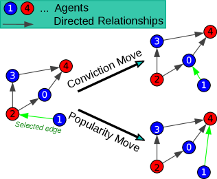
Figure 1: Illustration of the action of the model basic moves. Nodes represent agents and colors represent convictions. Edges represent directed social connections (A follows B if an edge is sent from A to B). The selected edge to be removed is in both cases $e_{1\to 2}$. In a conviction move, the new target can be chosen only among the blue nodes (in the sketch this move creates the edge $e_{1\to 0}$), while in a popularity move the new target can be chosen regardless of its opinion, so that every node with an in-degree greater than 0 is a potential candidate (in the sketch this moves creates the edge $e_{1\to 4}$).

II Definition of the model

Our model describes a social network as a directed graph where individuals (nodes) follow other individual’s opinions by sending directed edges to their corresponding nodes. The initial condition is a random directed graph $G_{0}(N,m,h)$ made of $N\in\mathbb{N}$ nodes. Each node has fixed outdegree $m\in\mathbb{N}$. A fraction $h\in[0;1]$ of individuals hold a certain conviction, which we identify with the color red (as opposed to the probability $1-h$ of holding the opposite conviction, i.e. being colored in blue). The total number of edges $M=N\cdot m$ defines the size of our system. The graph is constructed through the associated adjacency matrix by filling randomly with $m$ ones the matrix rows of a zero matrix (we exclude the matrix diagonal elements which would indicate self-edges). As a consequence of this construction procedure, the in-degrees follow a Poisson distribution with average value $m$ (as in an Erdõs-Rényi random graph Erdos and Rényi (1960)).

The network evolves at fixed conviction, by choosing at each step one of two possible rewiring moves (Fig. 1) accordingly to the choice parameter $\varphi\in[0;1]$ :

• with probability $\varphi$ a conviction move chooses randomly one among all the edges $e_{i\to j}$ between two nodes holding different convictions (which we will call “heterogeneous” edges), deletes, chooses uniformly a new target node $k$ holding the same conviction as $i$ and creates a new “homogeneous” edge $e_{i\to k}$;

• alternatively, with probability $1-\varphi$, a popularity move which chooses randomly one edge $e_{i\to j}$ among all the edges of the network, deletes it, and creates a new edge $e_{i\to k}$ with a target $k$ chosen among all the nodes with a preferential attachment criterion, i.e. with a probability equal to the in-degree of the target node normalized by the total number of edges $M$.

It is important to underline the fact that the opinion move selects the edge to be removed in the basket of the heterogeneous edges. As it will be more clear in the following, this choice is essential in order to obtain a threshold phenomenon for segregation.

We quantify the segregation using as order parameter the total number of homogeneous edges connecting nodes with the same conviction. In the initial condition ($t=0$), and for $M$ sufficiently large, the densities of the four different kinds of edges (red to red, blue to blue, red to blue and blue to red) are:

$$e_{0}(rr) =h^{2}$$

$$e_{0}(bb) =(1-h)^{2}$$

$$e_{0}(rb) =e_{0}(br)=h(1-h)\ \ .$$ (1)

More in general, for every step $t>0$, the link densities are functions of this parameter order parameter. Indeed, since $\Omega_{t}:=M(e_{t}(rr)+e_{t}(bb))$, one has

$$e_{t}(rr) =\frac{h^{2}}{h^{2}+(1-h)^{2}}\frac{\Omega_{t}}{M}$$

$$e_{t}(bb) =\frac{(1-h)^{2}}{h^{2}+(1-h)^{2}}\frac{\Omega_{t}}{M}$$

$$e_{t}(rb) =e_{0}(br)=\frac{M-\Omega_{t}}{2M}\ .$$ (2)

We define a segregated phase as a state where, for large networks, typically all the heterogeneous edges disappear, leaving the network with only edges between like-minded nodes, characterized by a saturation of the order parameter to the maximum value $\Omega_{t}=M$.

III Results

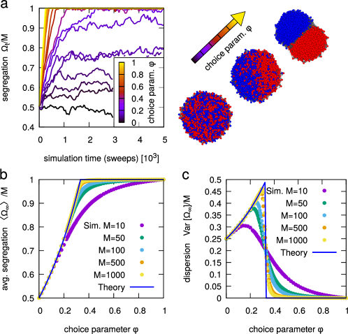
Figure 2: A threshold phenomenon to a segregated state appears for a critical value of the choice parameter $\varphi_{c}$. a) Evolution of the fraction of homogeneous links. The plot shows the order parameter normalized by the total number of edges $M$ plotted against sweeps. The curves are obtained by simulating the evolution of the same initial random graph $G_{0}(N=500,m=5,h=1/2)$ for different values of $\varphi$. For low $\varphi$, the long-time value of $\Omega_{\infty}(\varphi)$ relaxes to a steady state where the edges connecting nodes with different colors fluctuate around a finite value, while as $\varphi$ grows, it reaches one (a segragated state) in a finite time. The right-hand panel shows some illustrative simulation snapshots, where the network is visualized with a spring model based on shared links. b) Plot of the mean order parameter at steady state versus the choice parameter $\varphi$ comparing the analytical results (solid line) of Eq. 7 with numerical simulations for different sizes of the network $M$ (symbols). This analysis supports a segregation transition for $\varphi_{c}=1/3$ (for $h=1/2$). c) Fluctuations scale linearly with the size of the system. Plot of the dispersion of the order parameter from the simulations in panel b (symbols). As the size of the network grows, the variability across realizations peaks around the critical value $\varphi_{c}=1/3$ reflecting the prediction of Eq. 12 (solid line).

III.1 A transition to a segregated state emerges at a critical point

By construction of the model dynamics, conviction moves favor the transition to a segregated phase, while popularity moves try to reestablish the disorder and will also affect the in-degree distribution. Moreover, we expect networks characterized by asymmetric densities of opinions ($h\neq 1/2$) to reach a segregated phase more easily.

Starting by the same initial random graph $G_{0}$, we evolved the network for different values of $\varphi$ and at each step we recorded the order parameter $\Omega_{t}(\varphi)$, starting from initial conditions with $\Omega_{0}=1/2$ for $h=1/2$ (Fig. 2a), representing the fraction of homogeneous edges (connecting individuals with equal convictions). For low values of $\varphi$, the system does not segregate, but they reach a balance between popularity- and conviction-based moves. As the value of $\varphi$ increases, conviction-based moves become increasingly dominant, and the steady-state value of the order parameter increases until it reaches the maximum possible value $M$, indicating that typically the number of heterogeneous edges is negligible compared to the total number of edges, and the system reaches a segregated phase. This behavior suggests the existence of a critical value $\varphi_{c}$ of the choice parameter, above which the steady state of the network is always in a segregated phase.

In order to find the critical value of the choice parameter analytically, we used a mean-field approach, based on an estimate of the average variation $\Delta\Omega_{t}$ at every step. Conviction moves increase $\Omega_{t}$ by 1, while popularity moves might act differently depending on the probability of picking an edge of a certain kind, and also on the kind of the new edge created. The resulting mean-field equation is

$$\Delta\left<\Omega_{t}(\varphi,h)\right>=\underbrace{\vartheta\varphi}_{\text{conv. move}}+\underbrace{(1-\varphi)\left[\vartheta p_{t}^{+}(h)-p_{t}^{-}(h)\right]}_{\text{pop. move}}\ ,$$ (3)

where the Heaviside step function $\vartheta:=\theta(M-\Omega_{t})$ excludes forbidden moves once the segregation state is reached, while $p_{t}^{\pm}(h)$ are the probabilities of respectively increasing and decreasing the order parameter with a popularity move.

In the continuum time limit, and for $h=1/2$ (for a more general derivation for every $h\in[0;1]$ see section A.1) Eq. (3) gives the following differential equation for the average value of the order parameter

$$\partial_{t}\left<\Omega_{t}(\varphi)\right>=\vartheta\frac{1+\varphi}{2}-(1-\varphi)\frac{1+\vartheta}{2}\frac{\left<\Omega_{t}(\varphi)\right>}{M}\ .$$ (4)

This equation can be explicitly integrated (for $\varphi\neq 1$), yielding the time dependence for the average value of the order parameter,

$$\frac{\left<\Omega_{t}(\varphi)\right>}{M} =\left[\left(1-\frac{1}{2}\vartheta\right)-\frac{\vartheta}{1+\vartheta}\frac{1+\varphi}{1-\varphi}\right]e^{-(1-\varphi)\frac{1+\vartheta}{2M}t}+$$

$$+\frac{\vartheta}{1+\vartheta}\frac{1+\varphi}{1-\varphi}\ \ .$$ (5)

In the pre-segregation regime (where $\Omega_{t}<M$ and therefore $\vartheta=1$) the relaxation is then exponential with characteristic time

$$\tau_{\Omega}=\frac{M}{1-\varphi}.$$ (6)

Hence, the asymptotic value

$$\frac{\left<\Omega_{\infty}(\varphi)\right>}{M}=\min_{\varphi\in[0;1)}\left\{1,\frac{1+\varphi}{2(1-\varphi)}\right\}$$ (7)

will be reached for times $t\gg\tau_{\Omega}$. Fig. 2b compares this prediction with direct simulations. The model behaves as expected already for relatively small-sized networks ($M=100$) and gradually moves towards the predicted curve as the size of the system grows. By setting $\left<\Omega_{\infty}(\varphi)\right>=1$ in Eq. 7 and solving for $\varphi$ one finds the critical value of the choice parameter at which the transition occurs, which for $h=1/2$ is $\varphi_{c}=1/3$. This transition has a clear similarity with second order phase transitions Landau and Lifshitz (1980) , because of a discontinuity in the first derivative of $\Omega_{t}$ with respect to $\varphi$. The analogy identifies the order parameter $\Omega$ with the magnetization, while the role of the temperature is played here by the choice parameter $\varphi$.

The fluctuations of the order parameter also characterize the transition. These can be estimated by the second cumulant moment $\text{Var}[\Omega_{\infty}(\varphi)]$. A peak in amplitude of the fluctuations at the critical value $\varphi_{c}$ should signal the transition. In the social segregation interpretation, this means that the transition to a segregated state is also marked by sudden growth and shrinkage of its connections to the rest of the world. In order to access the fluctuations analytically, we explicitly considered the master equation Gardiner (1985)). Calling $P_{t}(\Omega)$ the probability of having $\Omega$ homogeneous edges at time $t$ the master equation is defined as

$$\partial_{t}P_{t}(\Omega)=\sum_{\Omega^{\prime}\neq\Omega}W(\Omega|\Omega^{\prime})P_{t}(\Omega^{\prime})-W(\Omega^{\prime}|\Omega)P_{t}(\Omega)\ ,$$ (8)

where $W(\Omega|\Omega^{\prime})$ are the transition rates of moving from a network with $\Omega^{\prime}$ homogeneous edges to a network of $\Omega$ edges, which for our system (always in the case of $h=1/2$) is

$$W(\Omega|\Omega^{\prime}) =\delta_{\Omega^{\prime},\Omega-1}\left[\varphi+(1-\varphi)\frac{M-\Omega^{\prime}}{2M}\right]+$$

$$+\delta_{\Omega^{\prime},\Omega+1}(1-\varphi)\frac{\Omega^{\prime}}{2M}+\delta_{\Omega^{\prime},\Omega}\frac{1-\varphi}{2}\ .$$ (9)

In the above equation, the first row describes the contribution of both the opinion and popularity moves to an increase in $\Omega$, while the second row describes the contributions of the popularity move to respectively decrease and keep unaltered the order parameter. Then we define the factorial moment generating function

$$G(s,t)=\sum_{\Omega=0}^{M}s^{\Omega}P_{t}(\Omega)\ ,$$ (10)

where $s\in\mathbb{R}$ is the dual parameter of $\Omega$. Combining Eqs. (8) and (10) (see Appendix A.2) yields the following partial differential equation,

$$\partial_{t}G(s,t)=G(s,t)\frac{1+\varphi}{2}\left(s-1\right)+\partial_{s}G(s,t)\frac{1-\varphi}{2M}\left(1-s^{2}\right)\ .$$ (11)

By evaluating $\partial_{s}^{n}[\partial_{t}G(s,t)|_{s=1}]$ for every $n\in\mathbb{N}$ we obtain a closed system of time-only differential equations giving the exact dynamics (including the transient phase) of all the factorial moments. The first factorial moment coincides with the average, so we find again Eq. 4, whereas the second factorial moment gives $\left<\Omega_{t}^{2}\right>$ and hence the variance. Taking the long-time limit we obtain an analytical expression for the fluctuations

$$\frac{\text{Var}[\Omega_{\infty}(\varphi)]}{M}=\begin{cases}\frac{1+\varphi}{4(1-\varphi)}&\text{for }\varphi\leq 1/3\\ 0&\text{for }\varphi>1/3\end{cases}$$ (12)

Fig. 2c shows that as the size of $M$ (number of edges) of the network grows, the simulations tend to agree with this large-$M$ prediction, showing a behavior that resembles that of the susceptibility in second-order phase transitions, with fluctuations amplitude scaling linearly in $M$.

By means of the generating function formalism, we can go further and calculate exactly the stationary solution of the Master Equation (8) with transition rates given by Eq. (III.1). The resulting stationary probability function $P_{\text{stat}}$ is (see Appendix A.3 for detailed calculations):

$$P_{\text{stat}}(\Omega)=\frac{2^{-\frac{M(\varphi+1)}{1-\varphi}}\left(\frac{M(\varphi+1)}{1-\varphi}\right)^{(\Omega)}}{\Omega!},$$ (13)

where $x^{(\Omega)}$ is the factorial power of $x$ and it is given by $\frac{\Gamma(x+1)}{\Gamma(-\Omega+x+1)}$. From Eq. (13) we can then define the entropy of the system $S(\varphi)=-\sum_{\Omega=0}^{M\rightarrow\infty}P_{\text{stat}}(\Omega)\log[P_{\text{stat}}(\Omega)]$ and its derivative with respect to the choice parameter $\varphi$. As Figure 3 shows, by plotting $S(\varphi)$ and $\partial_{\varphi}S(\varphi)$ we can effectively see that the system undergoes a genuine phase transition.

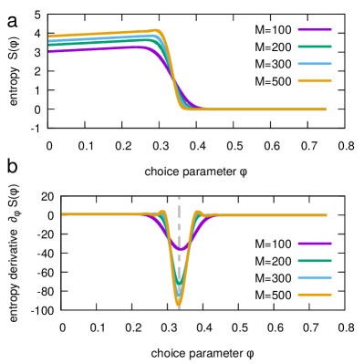
Figure 3: Entropy is characterized by a discontinuity in correspondence with the critical value of the choice parameter $\varphi_{c}$. A) The entropy of the system as a function of the order parameter $\varphi$ for different system size $M$. B) Its derivative with respect to $\varphi_{c}$. The dashed gray line represent the predicted critical threshold $\varphi_{c}=1/3$.

III.2 Overlap of time scales is necessary for a segregation transition to exist

We now discuss more in detail an essential ingredient for a segregation sharp transition to exist, the fact that the conviction move occurs on the same time scale of the popularity move, regardless of the size of heteorogeneous edges in the system. In other words, the conviction move is realized at each step with probability $\varphi$ drawing directly from the basket of heterogeneous edges in order to observe the transition.

We can understand this result by considering a similar model in which the opinion move is, for instance, defined as follows. Select an edge randomly among all the $M$ edges of the network (rather then from the basket of the heterogeneous ones) and if the edge is heterogeneous execute the conviction move, otherwise leave the network unaltered and move on by executing a new step. In this model the mean-field equation, Eq. 3 will take an additional term representing the heterogeneous edge density multiplying the conviction move term,

$$\Delta\left<\Omega_{t}\right>=\underbrace{\vartheta\varphi\frac{M-\left<\Omega_{t}\right>}{M}}_{\text{op. move variant}}+(1-\varphi)\left[\vartheta p_{t}^{+}(h)-p_{t}^{-}(h)\right]\ .$$ (14)

The critical value $\varphi_{c}$ is found setting $\Delta\left<\Omega_{t}\right>$ to zero and the average value of the order parameter saturates to its maximum value $M$. Substituting these quantities one immediately finds that the contribution of the opinion move disappears, leaving us with the equation $(1-\varphi_{c})\left[\vartheta p_{t}^{+}(h)-p_{t}^{-}(h)\right]=0$ which has the only trivial solution $\varphi_{c}=1$ (that represents a model in which only opinion based move are executed). In other words, a segregated phase is found only in the trivial case where the agents only choose their connections by conviction.

This analysis also gives a general condition for the existence of a transition, which is that the conviction move has to be such that the multiplicative factor introduced in the opinion move term in Eq. (14) translates into a function $f(\Omega_{t})$ characterized by the condition $f(M)\neq 0$). A possible justification for this forcing in the opinion move can be found by considering some realistic situations characterized by a segregation phenomenon driven by strong convictions (ethnicity, political orientation, religious beliefs, etc.). If an agent is left only with opposite minded neighbors, it is likely going to be the first one to decide to sever a connection and rewire with someone with the same conviction. For this reason, we believe that direct targeting of heterogeneous connection in an environment of strong convictions might be a realistic assumption.

III.3 The popularity move broadens the in-degree distribution in the unsegregated phase, but does not affect the transition point.

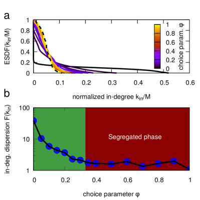
Figure 4: Preferential attachment from the popularity move broadens hte in-degree distribution. a) Empirical survival distribution function (ESDF) of the in-degree distributions of networks evolved for different values of $\varphi$. The plot was obtained by evolving an initial random graph $G_{0}(N=100,m=5,h=1/2)$ for $t=10^{6}$ steps (the in-degrees are normalized with respect to the total number of edges $M=500$). The broadening of the distribution indicates the increasing presence of bigger attractors in the evolved networks. b) Two different trends for the Fano factor of the in-degrees are observed in the regions below and above the segregation transition. The plot reports the Fano factor of the in-degrees distributions shown in panel a versus the choice parameter $\varphi$. In the region above the critical value of the choice parameter $\varphi_{c}=1/3$ the deviation from a Poisson distribution ($F(k_{in})=1$) is small, while the unsegregated region shows a super-exponential departure (the vertical axis is in log-scale) towards larger dispersions as $\varphi$ decreases.

We proceed by considering the role of the popularity move in setting the in-degree distribution and in the segregation transition. The initial random graph $G_{0}(N,m,h)$ has by definition Poisson-distributed in-degrees $k_{in}$ for large $N$, with a mean equal do the fixed outdegree of every node of the network $m$. As the network evolves, the distribution of the in-degrees changes at each popularity move, because the most popular nodes are more likely to be chosen as a target for the newly created edges. This determines a departure from the initial distribution towards heavier-tailed distributions, in analogy with the “rich gets richer” principle that usually characterizes social networks Castellano et al. (2009). In order to properly characterize this behavior evaluated the empirical survival distribution function (ESDF) of the in-degree distributions of evolved graphs $G_{t}$ for different values of the choice parameter. The ESDF indicates the probability of observing a node $i$ with in-degree $k_{in}(i)$ greater then a certain value $k_{in}$, and is defined as

$$\text{ESDF}(k_{in})=\frac{1}{M}\sum_{i=0}^{M}\theta(k_{in}-k_{in}(i))\ ,$$ (15)

Fig. 4a shows that when $\varphi=1$ the initial distribution is unaltered (the dashed line represents the distribution for the initial random graph $G_{0}$), but as $\varphi$ decreases the in-degree distributions take increasingly heavier tails.

The same phenomenon can be quantified by a single broadness parameter such as the Fano factor of the in-degrees $F(k_{in})$, defined as

$$F(k_{in})=\frac{\text{Var}[k_{in}]}{\left<k_{in}\right>}\ .$$ (16)

This parameter is 1 for a Poisson distribution, whereas greater values indicate larger dispersion. Fig. 4 shows this parameter plotted as a function of the choice parameter $\varphi$. The Fano Factor increases as popularity-based moves become more probable (as $\varphi$ goes to zero). Moreover two different trends appear to characterize the region below and above the critical value $\varphi_{c}=1/3$.

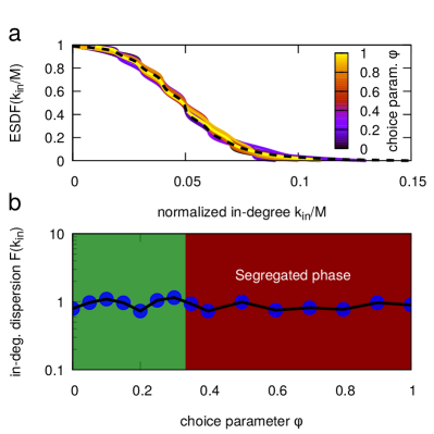
Figure 5: . Skewed node popularity does not affect segregation. ab) Same plots as Fig. 4, for a model in which the popularity move is changed with a rewiring on a uniformly chosen random node. This model shows the same phase transition as the original one (and in particular the plots in Fig. 2bc are identical), but the transition is not accompanied by changes in node degree.

Finally, although we found that popularity-based rewiring increases the dispersion of social connections in the unsegregated regime, this preferential attachment ingredient does not affect the segregation transition in any way, as we have verified by substituting popularity-based rewiring with random rewiring in our simulations (Fig. 5). Although one may expect that the presence of popular individuals may help avoiding the emergence of segregation due to their capacity of attracting new nodes regardless of their opinion, this does not happen in this model. The reason is easily understood from Eq. (3) and (14), which govern the dynamics of the order parameter, where it is clear that the in-degree distribution never comes into play.

III.4 Minority convictions segregate more easily

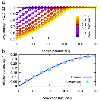
Figure 6: Minority convictions tend to segregate more easily. a) Average value of the order parameter $\left<\Omega_{t}\right>$ in networks evolved from initial networks $G_{0}(100,5,h)$ for different values of $h\leq 1/2$ (the results for $h>1/2$ are the same due to the symmetry $h\to 1-h$). As the the density of nodes holding a certain conviction decreases, the networks will reach a segregated phase for lower values of $\varphi$. b) Simulations confirm the analytical prediction for the critical points of the model. The critical points (symbols) are ectracted from the curves in panel a, for different values of $h$, and compared with the prediction described by Eq. 18 (solid line).

The results presented up to this point were obtained under the hypothesis of equally represented convictions condition ($h=1/2$). A more generic case describes minority versus majority convictions, characterized by different values of $h$. The differences from the symmetric case concern both the characteristic time $\tau_{\Omega}$ needed to reach the steady state and the critical value $\varphi_{c}$ at which the transition to a segregated phase occurs.

In order to study this asymmetric situation we write a mean-field equation valid for every value of $h\in[0,1]$. Starting from Eq. 3, we just need to specify how the terms $p^{\pm}_{t}(h)$ depend on $h$ (see section A.1),

$$p_{t}^{+}(h) =\frac{M-\left<\Omega_{t}\right>}{2M}$$

$$p_{t}^{-}(h) =\frac{h(1-h)}{h^{2}+(1-h)^{2}}\frac{\left<\Omega_{t}\right>}{M}\ .$$ (17)

The resulting mean-field equation can be integrated in the continuum limit as in the symmetric case $h=1/2$, yielding the dynamics of the average value of the order parameter. The critical value $\varphi_{c}$ on the asymmetry $h$ is obtained again by imposing the segregation regime conditions $\Delta\left<\Omega_{t}\right>=0$ and $\left<\Omega_{t}\right>=M$. Solving for $\varphi$ gives

$$\varphi_{c}(h)=\frac{h(1-h)}{1-h(1-h)}$$ (18)

for the critical value. This relation satisfies the red-blue symmetry $\varphi_{c}(h)=\varphi_{c}(1-h)$ with maximum value $\varphi_{c}(1/2)=1/3$ (as in Eq. 7) for the symmetric case. Fig. 6b compares the predicted critical point from Eq. 18 to simulations of evolved networks for different values of $h$ Fig. 6a. This analysis shows that a situation characterized by a minority conviction favors segregation for lower values of the choice parameter, indicating that the symmetric situation is the one in which segregation can be more easily avoided (the situation is analogous to the miscibility gap for phase segregation in a binary mixture).

The characteristic duration of the transient before a steady state is reached is also affected by the presence of a minority conviction. The solution of the mean-field equation gives

$$\tau_{\Omega}(h)=\frac{2M\left[h^{2}+(1-h)^{2}\right]}{1-\varphi}\ ,$$ (19)

i.e., the characteristic relaxation time will increase for asymmetric convictions. This time scale is important in cases where the segregation dynamics competes with the spreading of consensus Holme and Newman (2006); Durrett et al. (2012).

III.5 Scale-invariance close to the transition

The limit of large system size, $M\rightarrow\infty$, is better analyzed in terms of a finite-size scaling ansatz, typical of critical phenomena Fisher (1967); Hahne (2006). We define the normalized choice parameter

$$t=\frac{\varphi-\varphi_{c}}{\varphi_{c}}\ .$$ (20)

and the intensive order parameter

$$m=\frac{M-\Omega_{\infty}}{M}$$ (21)

so that

$$\langle m\rangle=1-\frac{\langle\Omega_{\infty}\rangle}{M}=\langle\frac{M-\Omega_{\infty}}{M}\rangle$$ (22)

and we assume that $\langle m\rangle$, which in principle depends on both $M$ and $t$ separately, is an homogeneous function of $t$ and a suitable power of $M$, that is

$$\langle m\rangle=|t|^{\beta}\tilde{f}_{1}(M^{y}t)$$ (23)

in the large (small) $M$ ($t$) limit with $M^{y}t$ fixed. $y$ and $\beta$ are exponents that are expected to be independent of the microscopic details of the dynamical model, characterizing the transition point, while $f$ is a scaling function, which might depend on the model specificities. Since we expect that $m$ is non-zero (zero) for $t<0$ ($t>0$) the scaling function $f$ should behave asymptotically as

$$\lim_{x\rightarrow+\infty}\tilde{f}_{1}(x)=0,\qquad\lim_{x\rightarrow-\infty}\tilde{f}_{1}(x)=\textrm{constant}>0$$ (24)

In order to estimate the two scaling exponents $\beta$ and $y$, we plot $m|t|^{-\beta}$ versus $M^{y}t$ and determine the exponents so that the best collapse of the different curves is obtained. Indeed one should obtain a different curve for each value of $M$ as $t$ varies and this is what we observe for generic pair $\beta$ and $y$. However for $\beta=1$ and $y=1/2$ the various curves collapse in a range of $x\equiv M^{y}t$ that increases as $M$ becomes larger and larger as Fig.7, panel (a), shows.

The same analysis leads to the following scaling ansatz for the variance of $m$ (corresponding to $\text{Var}[\Omega_{\infty}]/M^{2})$ in terms of the original extensive order parameter):

$$\text{Var}[m]=t^{2}\tilde{f}_{2}(M^{1/2}t)$$ (25)

and the corresponding collapse is shown in Fig.7, panel (b). Both scaling Eqs.(23) and (25) are captured by the more general scaling ansatz of the distribution function of $m$

$$P(m,t,M)=|t|^{-1}\tilde{P}(mt^{-1},\ M^{1/2}t)$$ (26)

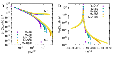
Figure 7: The fraction of homogeneous edges and its variance obey scaling. a) Scaling collapse for the fraction of homogenous edges. b) Scaling collapse for the variance. The $x$ and $y$ axes of both plots compare the functions predicted by Eqs. 23 and 25. The symbols correspond to data points from simulations at different network size above and below the segragation transition point.

III.6 A model with pure intra-specific aversion leads to an equivalent segregation threshold behavior.

Motivated by the literature on segregation models based on aversion between unlike individuals Schelling (1971); Henry et al. (2011), we asked whether the same threshold phenomenon observed in our model could be present in case of conviction moves that were based purely on aversion bias.

To this end, we defined a model variant where the conviction move (with probability $\varphi$) chooses randomly one heterogeneous edge, between two nodes holding different convictions and rewires it to a random node. In this variant, the popularity move (with probability $1-\varphi$ at each step) remains the same. Under this variant, Eq. (3) becomes

$$\Delta\left<\Omega_{t}(\varphi,h)\right>=\underbrace{\vartheta\frac{\varphi}{2}}_{\text{conv. move}}+\underbrace{(1-\varphi)\left[\vartheta p_{t}^{+}(h)-p_{t}^{-}(h)\right]}_{\text{pop. move}}\ ,$$ (27)

immediately leading to the expression,

$$\frac{\left<\Omega_{\infty}(\varphi)\right>}{M}=\min_{\varphi\in[0;1)}\left\{1,\frac{1}{2(1-\varphi)}\right\}$$ (28)

for the mean fraction of heterogeneous edges.

By setting $\left<\Omega_{\infty}(\varphi)\right>=1$ in Eq. 28 and solving for $\varphi$ one finds again the critical value, which for $h=1/2$ is $\varphi_{c}=1/2$. An analogous reasoning can be followed for solving for the higher moments of the distribution of $\Omega$. Fig. 8 shows that direct simulations of the aversion bias model are fully in line with these theoretical predictions. Thus, we conclude that aversion alone is sufficient to produce a sudden segregation threshold.

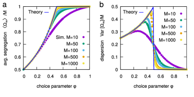
Figure 8: The sudden transition to a segregated state remains in a model with aversion bias only. a) Mean order parameter at steady state versus the choice parameter $\varphi$ comparing theory (solid line) with numerical simulations for different sizes of the network $M$ (symbols). This analysis supports a segregation transition for $\varphi_{c}=1/2$ (for $h=1/2$). b) The dispersion of the order parameter (symbols) shows the same behavior as the standard model (compare with Fig 2).

IV Discussion and Conclusions

Social segregation is ubiquitous in our society, and manifests itself as fragmentation of social networks at all scales, in countries, cities, schools, firms, governmental agencies, etc. Its consequences may lead to a wide range of nefastous phenomena ranging from inefficient planning to war. It is driven by diverse and enormously complex sociological, cultural, environmental and economic dilemmas, which are unlikely to be solved in the near future. However, since the pioneering work of Schelling Schelling (1969); Dall’Asta et al. (2008); Gauvin et al. (2010); Henry et al. (2011) there is increasing agreement that there may be common quantitative traits in the “macroscopic” dynamics of segregation that emerge from this complexity. A quantitative understanding of the consequences of such simple features on the dynamics of a social network may be important to develop efficient estimators to be used in real-life examples to detect and prevent segregation phenomena.

The framework developed here shows that complete segregation in a network setting without any spatial aspects can emerge as a threshold phenomenon that corresponds to a genuine phase transition. Close to such transition point, small perturbations of the system can cause very large rearrangements in the state. Importantly, we have shown that such transition point is scale invariant, hence “universal” in the statistical physics sense. This supports the hypothesis that close to this critical point more detailed descriptions of social interactions are not necessary, since a wide class of models may behave similarly.

We can also parallel this model with available physical models for the separation of phases and mixtures. For example, binary mixtures can be described in a coarse-grained way as a set of particles of two kinds filling a cubic lattice, with an energy cost for particles of one kind sitting next to particles of the other kind. This system (equivalent to an Ising model) shows a spatial phase separation when temperature is lowered. Contrary to this case, in our model set on a network a concept of distance is missing, since all individuals can potentially interact with any other agent in each move. However, we can parallel our results to a variant of the above model where instead of the usual “local” fraction of lattice sites occupied by each kind of particle, we write the free energy in terms of the parameter used here, i.e., the fraction of homogeneous edges $e_{h}=-\Omega/M$. The energetic term is simply $-\chi e_{h}$. In order to write the entropy, we consider the network as a gas of edges formed by connecting nodes. We compute the number of ways to assign $\Omega$ edges out of $M$, considering that each edge is spurious if two colors of the same kind are selected. The resulting free energy is $\beta F=e_{h}\log(e_{h})+(1-e_{h})\log(1-e_{h})-e_{h}\chi$. Minimizing this free energy and comparing with the equations governing our model shows that they are different, and our model cannot be reconducted to this simple case. The question remains open on whether there is a simple equilibrium model recapitulating the phase-separation behavior shown by our segregation model.

Segregation in social networks may be driven by both homophyly (the choice of social interactions with like individuals) and aversion. These ingredients are mixed in different proportion in the existing literature. Our basic model contains both, since in the conviction-based rewirings interactions between dissimilar partners are rewired in favor of homogeneous ones. Schelling’s model Schelling (1971) shows that aversion from dissimilar network partners alone, coupled with a random selection of new partners, may be sufficient to induce segregation. Our analysis of a model variant where the conviction-based rewiring is based on pure aversion supports this conclusion. Indeed, this variant shows the same type of threshold phenomenon, in full quantitative agreement with the main model. The (expected) quantitative change is that in the case of pure aversion the transition point is shifted to higher values of the choice parameter $\varphi$, compared to the case where both aversion and homophyly are in place.

Overall, our analysis supports the conclusion that whether conviction-based rewiring is based on aversion or homophyly is not a key ingredient for the existence of a segregation threshold. Instead, the important feature to determine a threshold phenomenon for segregation is that the the conviction-based rewiring of the network (based on aversion or homophyly, or both) occurs on the same time scale of the popularity-based rewirings (i.e. the establishment of social interactions that are non-discriminant). In the alternative scenario in which, e.g., each kind of rewiring occurs proportionally to the number of extant interactions, segregation occurs smoothly. In such situation, at all levels of the bias in establishing interactions (quantified by the choice parameter $\varphi$) the network maintains a finite fraction of interactions between dissimilar individuals.

Appendix A Analytical calculations

This section presents in further detail the two different methods used to derive the analytic expressions for the cumulants of the order parameter (namely equations 7 and 12).

A.1 Mean-field approach

As previously explained, the mean-field approach consists in quantifying the average variation of the order parameter at every step of the dynamics, which resulted in equation 3. The meaning of the terms of such equation have already been discussed, here we will present the more general derivation of the contributions $p_{t}^{\pm}(h)$ for every $h\in[0,1]$, which will yield the more general solution of equation III.1 for different densities of colored nodes.

The terms $p_{t}^{\pm}(h)$ represent the probabilities of, respectively, increasing and decreasing the order parameter $\Omega$ when a popularity move is performed:

$$p_{t}^{+}(h) =\mathrm{Prob}\left[e_{t}(rb)\to e_{t}(rr)\right]+\mathrm{Prob}\left[e_{t}(br)\to e_{t}(bb)\right]$$

$$p_{t}^{-}(h) =\mathrm{Prob}\left[e_{t}(rr)\to e_{t}(rb)\right]+\mathrm{Prob}\left[e_{t}(bb)\to e_{t}(br)\right]$$ (29)

which are found to be

$$p_{t}^{+}(h) =\frac{M-\langle\Omega_{t}(\varphi,h)\rangle}{2M}$$

$$p_{t}^{-}(h) =\frac{\langle\Omega_{t}(\varphi,h)\rangle}{M}\frac{h(1-h)}{h^{2}+(1-h)^{2}}\ .$$ (30)

By substituting these coefficients in equation III.1 and taking the continuous-time limit we obtain the following differential equation,

$$\partial_{t}\langle\Omega_{t}(\varphi,h)\rangle=\vartheta\frac{1+\varphi}{2}-\\ (1-\varphi)\frac{2h(1-h)(1-\vartheta)+\vartheta}{2\left(h^{2}+(1-h)^{2}\right)}\frac{\langle\Omega_{t}(\varphi,h)\rangle}{M}\ ,$$ (31)

which can be explicitly integrated in time (for $\varphi\neq 1$), yielding

$$\frac{\langle\Omega_{t}(\varphi,h)\rangle}{M}=\left[1+\vartheta\left(\frac{\langle\Omega_{0}(\varphi,h)\rangle}{M}-1\right)-\vartheta\frac{1+\varphi}{2}\alpha(\varphi,h)\right]\cdot\\ \cdot e^{-\frac{t}{\alpha(\varphi,h)}}+\vartheta\frac{1+\varphi}{2}\alpha(\varphi,h)\ ,$$ (32)

where the initial condition is

$$\frac{\langle\Omega_{0}(\varphi,h)\rangle}{M}=e_{0}(rr)+e_{0}(bb)=h^{2}+(1-h)^{2}$$ (33)

and the coefficient $\alpha$ is

$$\alpha(\varphi,h)=\frac{2(h^{2}+(1-h)^{2})}{(1-\varphi)(2h(1-h)(1-\vartheta)+\vartheta)}\ .$$ (34)

If we evaluate this coefficient in the unsegregated phase (where $\vartheta\equiv 1$), we obtain the characteristic time of the transient phase, which is

$$\tau(\varphi,h)=\frac{2(h^{2}+(1-h)^{2})}{1-\varphi}$$ (35)

Taking the limit $t\to\infty$ of equation 32 yields the steady-state solution of the order parameter, which for every $\varphi\in[0,1)$ and $h\in[0,1]$ is,

$$\frac{\langle\Omega_{t}(\varphi,h)\rangle}{M}=\min\left\{1,\frac{1+\varphi}{1-\varphi}\left(h^{2}+(1-h)^{2}\right)\right\}\ .$$ (36)

Fig. 6 shows the phase diagram for $\langle\Omega_{t}\rangle$, which is in agreement with the fact that the critical value of the choice parameter $\varphi_{c}$ becomes lower as we move away from the symmetric nodes density given by $h=1/2$ (discussed in section III.4).

A.2 Master equation and moment-generating function approach

This section treats in further detail the derivation of a generic factorial moment of the order parameter $\Omega$. Substituting the rates III.1 in the master equation 8 one gets,

$$\partial_{t}P_{t}(\Omega) =P_{t}(\Omega-1)\left[\varphi+(1-\varphi)\frac{M-\Omega+1}{2M}\right]+$$

$$+P_{t}(\Omega+1)(1-\varphi)\frac{\Omega+1}{2M}-P_{t}(\Omega)\frac{1+\varphi}{2}$$ (37)

In order to find a differential equation for the FMGF 10 we first multiply by $s^{\Omega}$ both sides of equation A.2, and then we sum over the order parameter $\Omega$ itself. The probabilities $P_{t}(\Omega)$ are obviously defined only for $\Omega\in[0,M]$, so we need to explicitly set $P_{t}(\Omega)\equiv 0$ when $\Omega$ is outside that range. This notation has a practical advantage that allows us to extend the summation over $\Omega$ from the range $[0,M]$ to the range $[-1,M+1]$. This frees from border-term issues when re-indexing the summation for the terms on the right side. To evaluate the contribution with the $P_{t}(\Omega-1)$ coefficient, we set $\Omega^{\prime}=\Omega-1$ and obtain

$$\sum_{\Omega^{\prime}=-2}^{M}s^{\Omega^{\prime}+1}P_{t}(\Omega^{\prime})\left[\frac{1+\varphi}{2}-\frac{\Omega^{\prime}}{2M}\right]=\\ =\left[s\frac{1+\varphi}{2}-\frac{1-\varphi}{2M}s^{2}\partial_{s}\right]G(s,t)\ ,$$ (38)

where we introduced a derivative in $s$ in order to eliminate the multiplicative $\Omega^{\prime}$ in the summation. The same trick can be used for the $P_{t}(\Omega+1)$ term (this time we set $\Omega^{\prime}=\Omega+1$):

$$\sum_{\Omega^{\prime}=0}^{M+2}s^{\Omega^{\prime}-1}(1-\varphi)P(\Omega^{\prime})\frac{\Omega^{\prime}}{M}=\frac{1-\varphi}{2M}\partial_{s}G(s,t)$$ (39)

Finally, the $P_{t}(\Omega)$ term does not require any re-indexing and immediately yields $G(s,t)(1+\varphi)/2$. Putting all the pieces together we finally find the desired equation 11 for the dynamics of the FMGF.

Equation 11 is a partial differential equation that contains derivatives both in $s$ and $t$. Since we are only interested in finding the moments of the equation, we can avoid solving it explicitly: if we evaluate $\partial_{s}^{n}[\partial_{t}G(s,t)|_{s=1}]$ for every $n\in\mathbb{N}$ we obtain a closed system of time-only differential equations for the dynamics of the moments. In fact we can easily see that

$$\partial_{s}^{n}G(s,t)|_{s=1}=\langle\frac{\Omega!}{(\Omega-n)!}\rangle$$ (40)

For $n=1$, we are evaluating the first factorial moment, which coincides with the average. A straightforward calculation shows that we obtain precisely equation 4 (in the unsegregated phase with $\vartheta\equiv 1$). For $n=2$, we find the equation of the second factorial moment $\langle\Omega(\Omega-1)\rangle=\langle\Omega^{2}\rangle-\langle\Omega\rangle$, which reads

$$\partial_{t}\langle\Omega^{2}\rangle-\partial_{t}\langle\Omega\rangle=-2\frac{1-\varphi}{M}\langle\Omega^{2}\rangle+\left(1+\varphi+\frac{1-\varphi}{M}\right)\langle\Omega\rangle$$ (41)

By evaluating the steady-state solution ($\partial_{t}\langle\Omega^{2}\rangle=\partial_{t}\langle\Omega\rangle=0$) of this equation and substituting the steady-state form of $\langle\Omega\rangle$, we find the steady-state equation of $\langle\Omega^{2}\rangle$, which in turn gives us the variance

$$\mathrm{Var}\left[\Omega\right]=\langle\Omega^{2}\rangle-\langle\Omega\rangle^{2}=\frac{1+\varphi}{4(1-\varphi)}\ .$$ (42)

This equation coincides with the one presented in equation 12 (in the unsegregated phase).

A.3 Full Stationary Solution

Starting from the Master Equation (A.2) we can write the full equation for the Generating Function $G(s,t)$

$$\partial_{t}G(s,t)=aG(s,t)(s-1)+b\partial_{s}G(s,t)\left(1-s^{2}\right)\ ,$$ (43)

where $a=\frac{1+\varphi}{2}$ and $b=\frac{1-\varphi}{2M}$; $M$ is the total number of links. We assume the initial condition ($P(\Omega,t=0)=\delta_{\Omega-M/2}$ and thus we have $G(s,0)=s^{M/2}$. Additionally, the normalisation condition fixes $G(1)=1$.

The stationary solution for Eq. (43) is simple to find by solving directly the PDE, and leads to

$$G(s)=\left(\frac{1+s}{2}\right)^{a/b}\ .$$ (44)

In order to solve the full transient of the PDE (43) we use the so-called method of characteristics. Setting $f(s)=-b\left(1-s^{2}\right)$, then Eq. (43) corresponds to the following system of differential equations:

$$\dot{s}(t) = f(s)$$ (45)

$$\frac{d}{dt}G(s(t),t) = a(s(t)-1)G(s(t),t)\ .$$ (46)

Eq. (45) leads to the integral equation $-\int_{s(0)}^{s}\frac{dz}{1-z^{2}}\,dz=\int_{0}^{t}bdt$ where $s$ it evaluated at a final time $t$, i,e, $s(t)=s$. Solving this equation leads to

$$s=\frac{\text{Cosh}(bt)s(0)-\text{Sinh}(bt)}{\text{Cosh}(bt)-s(0)\text{Sinh}(bt)}$$ (47)

and

$$s(0)=\frac{s\text{Cosh}(bt)+\text{Sinh}(bt)}{\text{Cosh}(bt)+s\text{Sinh}(bt)}\ .$$ (48)

Finally, performing the integral $\int_{s(0)}^{s}a(s(\tau)-1)d\tau$ we find

$$G(s,t)=e^{-at}(\text{Cosh}(bt)+s\text{Sinh}(bt))^{a/b}\cdot\\ \cdot\left(\frac{s\text{Cosh}(bt)+\text{Sinh}(bt)}{\text{Cosh}(bt)+s\text{Sinh}(bt)}\right)^{M/2}\ .$$ (49)

In the limit t$\to\infty$, this expression gives the stationary solution Eq. (44). Expanding this in series around $s=0$, and matching term by term, one can find the transient solution $P(\Omega,t)$. In fact, we have that $G(s,t)=P(0,t)+sP(1,t)+...+s^{M}P(M,t)$ and $G(0,t)=P(0,t)$. Expanding the steady state solution of $G(s)$ in series around $s=0$, we obtain $G(s)=\sum_{\Omega=0}^{M}\frac{\partial_{s}^{\Omega}G(s)_{|s=0}}{\Omega!}s^{\Omega}$ leading to Eq. (13) in the main text. We highlight that Eq. (13) only holds for $\varphi\in[0,\varphi_{c})$.