Double charmonium productions in electron-positron annihilation using Bethe-Salpeter approach

¹Department of Physics, Samara University,P.O.Box 132, Samara, Ethiopia
²Department of Physics, University Institute of Sciences, Chandigarh University, Mohali-140413, India
Abstract
We calculate the double charmonium production cross section within the framework of $4\times 4$ Bethe-Salpeter Equation in the electron-positron annihilation, at center of mass energy $\sqrt{s}=10.6$GeV, that proceeds through the exchange of a single virtual photon. In this calculation, we make use of the full Dirac structure of 4D BS wave functions of these charmonia, with the incorporation of all the Dirac covariants (both leading and sub-leading). The calculated cross-sections for the double charmonium productions for final states, ($J/\Psi,\eta_{c}$); ($\Psi^{\prime},\eta_{c}$) ; ($J/\Psi,\eta_{c}^{\prime}$); and ($\Psi^{\prime},\eta_{c}^{\prime}$) are close to experimental data, and in broad agreement with results of other theoretical models.

1 Introduction

One of the challenging problems in heavy-quark physics is the process of double charmonium production in electron-positron annihilation at B-factories [1, 2, 3, 4]. Many studies of double quarkonium production process [5, 6, 7, 9, 8] have been preformed in order to understand this process, and thereby the internal structures of quarkonia and interactions of the quark and anti-quark inside the quarkonium. In recent years the quarkonium production has been studied in various processes at B-factories whose measurements were made by Babar and Belle collaborations [1, 2, 3, 4]. Among them, the study of charmonium production in $e^{+}e^{-}$ annihilation is particularly interesting in testing the quarkonium production mechanisms at center of mass energies $\sqrt{s}=10.6GeV$. The investigation of double charmonium production is very important since these charmonium can be easily produced in experiments and hence their theoretical prediction can verify the discrepancy between different theoretical models and experimental data. As regards the dynamical framework, to investigate the double charmonium production is concerned, many approaches have been proposed to deal with the cross - section of double charmonium production [5, 6, 7, 9, 8] and the pseudoscalar and vector charmonium production process has been recently studied in a Bethe-Salpeter formalism [10, 11]. However, in these studies the complete Dirac structure of P (pseudoscalar)and V (vector) quarkonia was not taken into account, and calculations were performed by taking only the leading Dirac structures, $\gamma_{5}$, and $i\gamma.\varepsilon$ in the BS wave functions of pseudoscalar and vector charmonia respectively.

In these calculations, we make use of the Bethe-Salpeter equation (BSE) approach [12, 13, 14, 15, 16], which is a conventional approach in dealing with relativistic bound state problems. Due to its firm base in quantum field theory, and being a dynamical equation based approach, it provides a realistic description for analyzing hadrons as composite objects, and can be applied to study not only the low energy hadronic processes, but also the high energy production processes involving quarkonia as well.

In our recent works [17, 18, 19, 20], we employed BSE under Covariant Instantaneous Ansatz, which is a Lorentz- invariant generalization of Instantaneous Approximation, to investigate the mass spectra and the transition amplitudes for various processes involving charmonium and bottomonium. The BSE framework using phenomenological potentials can give consistent theoretical predictions as more and more data are being accumulated. In our studies on $4\times 4$ BSE, in all processes except in [19], the quark - anti quark loop involved a single hadron-quark vertex, which was simple to handle. However for the transitions such as $V\rightarrow P+\gamma$ (where $V$ vector and $P$ pseudoscalar quarkonium), which we have studied in [19] and for the process of double charmonium production, $e^{+}e^{-}\rightarrow V+P$, we will study in present work, the process requires calculation involving two hadron-quark vertices, due to which the calculation becomes more and more difficult to handle. However in the present work, we demonstrate an explicit mathematical procedure for handling this problem using the formulation of $4\times 4$ Bethe - Salpeter Equation under Covariant Instantaneous Ansatz. We will use this framework for the calculation of cross section for the production of double charmonia, $(J/\psi,\eta_{c}),(J/\psi,\eta^{\prime}_{c}),(\psi^{\prime},\eta_{c})$, and $(\psi^{\prime},\eta^{\prime}_{c})$ in electron-positron annihilation that proceeds through a single virtual photon at center of mass energies, $\sqrt{s}=10.6$ GeV., where such problems do not enter in our previous papers on $4\times 4$ BSE. [17, 18, 19, 20, 21, 22].

This paper is organized as follows. In section 2, We introduce the detailed formulation of the transition amplitudes for the process of double charmonium production and the numerical results of cross - sections. Finally, we give the discussions and conclusions in section 3.

2 Formulation of double charmonium production amplitude

We start from the lowest order Feynman diagrams for the process, $e^{+}e^{-}\rightarrow V+P$, as given in Fig.1. There are four Feynman diagrams for the production of double charmonium, one of which is shown in Fig.1, while the other three can be obtained by reversing the arrows of the quark lines.

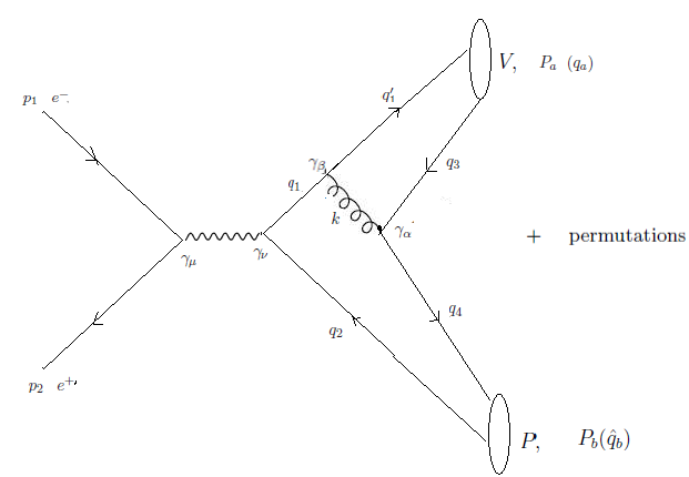
Figure 1: Leading order Feynman diagrams for the production of double charmonium in $e^{+}e^{-}$- annihilation.

The relativistic amplitude $M^{1}_{fi}$ for double charmonium production, corresponding to Fig.1, is given by the one-loop momentum integral as:

$$M^{1}_{fi}=\frac{2^{7}\pi^{2}\alpha_{em}\alpha_{s}}{3^{2}s}\left[\overline{\nu}(p_{2})\gamma_{\mu}u(p_{1})\right]\int\frac{d^{4}q_{a}}{(2\pi)^{4}}\int\frac{d^{4}q_{b}}{(2\pi)^{4}}Tr[\overline{\Psi}(P_{a},q_{a})\gamma_{\beta}S_{F}(q_{1})\gamma_{\mu}\overline{\Psi}(P_{b},q_{b})\gamma_{\beta}]\frac{1}{k^{2}}$$ (1)

where, $s$ is the Mendelstam variable defined as, $s=-(p_{1}+p_{2})^{2}$, $\alpha_{em}=\frac{e^{2}}{4\pi}$ is called the electromagnetic coupling constant and $\alpha_{s}=\frac{g^{2}_{s}}{4\pi}$ is the strong coupling strength, $\overline{\Psi}(P_{a},q_{a})$ and $\overline{\Psi}(P_{b},q_{b})$ are the conjugations of the BS wave function of vector and pseudoscalar charmonium respectively. From the figure, we can relate the momenta of the quark and anti-quark respectively as:

$$q^{\prime}_{1}=\frac{1}{2}P_{a}+q_{a}$$

$$q_{3}=\frac{1}{2}P_{a}-q_{a}$$

$$q_{4}=\frac{1}{2}P_{b}+q_{b}$$

$$q_{2}=\frac{1}{2}P_{b}-q_{b}$$ (2)

and the momenta for the propagators of gluon and quark are given respectively by:

$$k=\frac{1}{2}(P_{a}+P_{b})-q_{a}+q_{b}$$

$$q_{1}=P_{a}+\frac{1}{2}P_{b}+q_{b}$$ (3)

As the quark and gluon propagators depend upon the internal hadron momenta $q_{a}$ and $q_{b}$, the calculation of amplitude is going to involve integrations over these internal momenta and will be quite complex. Hence following Ref. [17, 18, 19], we simplify the calculation, by reducing the 4-dimensional expression of BS amplitude, $M^{1}_{fi}$ into 3-dimensional expression of BS amplitude, $M^{1}_{fi}$ and employing the heavy quark approximation on the propagators, the momenta $k$ and $q_{1}$ can be written as, $k\approx\frac{1}{2}(P_{a}+P_{b})$ and $q_{1}\approx P_{a}+\frac{1}{2}P_{b}$, which leads to, $k^{2}\approx\frac{s}{4}$ and $q^{2}_{1}\approx\frac{s}{2}+m_{c}^{2}$ [10, 11]. Then, with the above approximation and applying the definition of 3D BS wave function in [17, 18, 19, 20] $\psi(\hat{q}_{a})=\frac{i}{2\pi}\int M_{a}d\sigma\Psi(P_{a},q_{a})$ and $\psi(\hat{q}_{b})=\frac{i}{2\pi}\int M_{b}d\sigma_{b}\Psi(P_{b},q_{b})$, the double charmonium production BS amplitude, $M^{1}_{fi}$ can be written in the instantaneous Bethe-Salpeter amplitude form as:

$$M^{1}_{fi}=-\frac{2^{10}\pi^{2}\alpha_{em}\alpha_{s}}{3^{2}s^{3}}\left[\overline{\nu}(p_{2})\gamma_{\mu}u(p_{1})\right]\int\frac{d^{3}\widehat{q}_{a}}{(2\pi)^{3}}\int\frac{d^{3}\widehat{q}_{b}}{(2\pi)^{3}}Tr[\overline{\psi}(\widehat{q}_{a})\gamma_{\beta}(-i\not{P_{a}}-\frac{i}{2}\not{P_{b}}+m_{c})\gamma_{\mu}\overline{\psi}(\widehat{q}_{b})\gamma_{\beta}]$$ (4)

where $\psi(\hat{q}_{a})$ and $\psi(\hat{q}_{b})$ are the relativistic BS wave function of pseudoscalar and vector charmonium respectively. We now give details of calculation of double charmonium production for the process, $e^{+}e^{-}\rightarrow V+P$ in the next section.

• For the production process, $e^{+}+e^{-}\rightarrow V+P$
  The relativistic BS wave function of pseudoscalar and vector charmonium are taken from our recent papers [17, 18, 19] respectively as:

  $$\psi_{P}(\hat{q}_{b})=N_{P}[M_{b}+\not{P}_{b}+\frac{\not{\hat{q}_{b}}\not{P}_{b}}{m_{c}}]\gamma_{5}\phi_{P}(\hat{q}_{b})$$ (5)

  for $P_{b}$ and $M_{b}$, is the momentum and mass of the pseudoscalar charmonium respectively and $N_{P}$ is the BS normalization of the pseudoscalar charmonium, which is given in a simple form as:

  $$N_{P}=\left[\frac{16M_{b}}{m_{c}}\int\frac{d^{3}\hat{q}_{b}}{(2\pi)^{3}}\frac{\hat{q}_{b}^{2}}{\omega_{b}}\phi_{P}^{2}(\hat{q}_{b})\right]^{-1/2}$$ (6)

  and

  $$\psi_{V}(\hat{q}_{a})=N_{V}[M_{a}\not{\varepsilon}+\hat{q}_{a}.\varepsilon\frac{M_{a}}{m_{c}}+\not{\varepsilon}\not{P}_{a}+\frac{\not{P}_{a}\hat{q}_{a}.\varepsilon}{m_{c}}-\frac{\not{P}_{a}\not{\varepsilon}\not{\hat{q}_{a}}}{m_{c}}]\phi_{V}(\hat{q}_{a})$$ (7)

  were, $\varepsilon$ is the polarization vector of the vector quarkonia, $P_{a}$ and $M_{a}$, is the momentum and mass of the vector quarkonia respectively and $N_{V}$ is the BS normalization of the vector quarkonia, which is given in a simple form as:

  $$N_{V}=\left[16m_{c}M_{a}\int\frac{d^{3}\hat{q}_{a}}{(2\pi)^{3}}\frac{\hat{q}_{a}^{2}}{\omega_{a}^{3}}\phi_{V}^{2}(\hat{q}_{a})\right]^{-1/2}$$ (8)

  where $\phi_{P}(\hat{q}_{b})$ and $\phi_{V}(\hat{q}_{a})$ are the radial wave functions of $P$ and $V$, which are solutions of the 3D BSE for pseudoscalar and vector quarkonia respectively (see Ref.[18]). The adjoint BS wave functions for pseudoscalar and vector charmonia are obtained from $\overline{\psi}_{P,V}(\hat{q}_{b,a})=\gamma^{0}(\psi_{P,V}(\hat{q}_{b,a}))^{+}\gamma^{0}$. With the substitution of adjoint BS wave functions of $P$ and $V$ charmoni into the 3D amplitude Eq.(4), $M^{1}_{fi}$ becomes:

  $$M^{1}_{fi}=-\frac{2^{10}\pi^{2}\alpha_{em}\alpha_{s}}{3^{2}s^{3}}\left[\overline{\nu}(p_{2})\gamma_{\mu}u(p_{1})\right]\int\frac{d^{3}\widehat{q}_{a}}{(2\pi)^{3}}N_{V}\phi_{V}(\hat{q}_{a})\int\frac{d^{3}\widehat{q}_{b}}{(2\pi)^{3}}N_{P}\phi_{P}(\hat{q}_{b})[TR]$$ (9)

  were

  $$[TR]=Tr[(-M_{a}\not{\varepsilon}+\hat{q}_{a}.\varepsilon\frac{M_{a}}{m_{c}}-\not{\varepsilon}\not{P}_{a}-\frac{\not{P}_{a}\hat{q}_{a}.\varepsilon}{m_{c}}+\frac{\not{\hat{q}_{a}}\not{\varepsilon}\not{P}_{a}}{m_{c}})\gamma_{\beta}(-i\not{P_{a}}-\frac{i}{2}\not{P_{b}}+m_{c})\gamma_{\mu}(M_{b}+\not{P}_{b}+\frac{\not{\hat{q}_{b}}\not{P}_{b}}{m_{c}})\gamma_{5}\gamma_{\beta}].$$ (10)

  Applying the trace theorem and evaluating trace over the gamma matrices, one can obtain the expression:

  $$\left[TR\right]= -8M_{a}\epsilon_{\nu\delta\mu\lambda}\varepsilon_{\nu}P_{a\lambda}P_{b\delta}+\frac{8i}{m_{c}}\left[(\hat{q}_{a}.\varepsilon)\epsilon_{\lambda\delta\sigma\mu}P_{a\lambda}P_{b\beta}\hat{q}_{b\sigma}+\epsilon_{\rho\nu\lambda\phi}(P_{b\phi}\hat{q}_{b\mu}-P_{b\mu}\hat{q}_{b\phi})\right]$$ (11)

  $$\frac{8(\hat{q}_{a}.\varepsilon)M_{a}}{m_{c}^{2}}\left[\epsilon_{\mu\sigma\beta\delta}P_{a\beta}P_{b\delta}\hat{q}_{b\sigma}+\epsilon_{\lambda\beta\mu\sigma}P_{a\lambda}P_{b\beta}\hat{q}_{b\sigma}\right]+\frac{16M_{b}^{2}}{m_{c}}\epsilon_{\nu\delta\sigma\mu}\varepsilon_{\nu}P_{b\delta}\hat{q}_{b\sigma}$$

  $$-\frac{8(\hat{q}_{a}.\varepsilon)}{m_{c}}\epsilon_{\lambda\delta\sigma\mu}P_{a\lambda}P_{b\delta}\hat{q}_{b\sigma}+8iM_{b}\epsilon_{\rho\nu\lambda\mu}\varepsilon_{\nu}P_{a\lambda}\hat{q}_{a\rho}$$

  After some mathematical steps, we can get the following expression:

  $$\left[TR\right]=-16m_{c}\epsilon_{\mu\nu\rho\sigma}\varepsilon_{\mu}P_{a}^{\rho}P_{b}^{\sigma}$$ (12)

  Thus we can express the amplitude $M^{1}_{fi}$ for the vector and pseudoscalar charmonium production as:

  $$M^{1}_{fi}=\frac{2^{14}\pi^{2}\alpha_{em}\alpha_{s}m_{c}}{3^{2}s^{3}}\left[\overline{\nu}(p_{2})\gamma_{\mu}u(p_{1})\right]\epsilon_{\mu\nu\rho\sigma}\varepsilon_{\mu}P_{a}^{\rho}P_{b}^{\sigma}\int\frac{d^{3}\widehat{q}_{a}}{(2\pi)^{3}}N_{V}\phi_{V}(\hat{q}_{a})\int\frac{d^{3}\widehat{q}_{b}}{(2\pi)^{3}}N_{P}\phi_{P}(\hat{q}_{b})$$ (13)

  The full amplitude for the process $e^{+}+e^{-}\rightarrow V+P$, can be obtained by summing over the amplitudes of all the possibilities in Fig. 1. Then, the unpolarized total cross-section is obtained by summing over various $V+P$, spin-states and averaging over those of the initial state $e^{+}e^{-}$, which is given as:

  $$\sigma=\frac{1}{32\pi}\frac{\sqrt{s-16m^{2}_{c}}}{s^{3/2}}\int\frac{1}{4}\sum_{spin}|M_{total}|^{2}d\cos\theta$$ (14)

  The total amplitude, $|M_{total}|^{2}$ is given as:

  $$\frac{1}{4}\sum_{spin}|M_{total}|^{2}=\frac{2^{30}\pi^{4}\alpha_{em}^{2}\alpha_{s}^{2}m^{2}_{c}}{3^{4}s^{5}}\left[\int\frac{d^{3}\widehat{q}_{a}}{(2\pi)^{3}}N_{V}\phi_{V}(\hat{q}_{a})\right]^{2}\left[\int\frac{d^{3}\widehat{q}_{b}}{(2\pi)^{3}}N_{P}\phi_{P}(\hat{q}_{b})\right]^{2}$$ (15)

  After integration over the phase space, the total cross-section for vector and pseudoscalar charmonium production is:

  $$\sigma_{e^{+}e^{-}\rightarrow VP}=\frac{2^{27}\pi^{3}\alpha_{em}^{2}\alpha_{s}^{2}m^{2}_{c}}{3^{4}s^{4}}\left(1-\frac{16m^{2}_{c}}{s}\right)^{\frac{3}{2}}\left[\int\frac{d^{3}\widehat{q}_{a}}{(2\pi)^{3}}N_{V}\phi_{V}(\hat{q}_{a})\right]^{2}\left[\int\frac{d^{3}\widehat{q}_{b}}{(2\pi)^{3}}N_{P}\phi_{P}(\hat{q}_{b})\right]^{2}$$ (16)

  The algebraic expressions of the wave functions of pseudoscalar and vector charmonium, $\phi_{P(V)}(\hat{q}_{b(a)})$, for ground (1S) and first excited (2S) states respectively, that are obtained as analytic solutions of the corresponding mass spectral equations of these quarkonia in an approximate harmonic oscillator basis are [18]:

  $$\phi_{P(V)}(1S,\hat{q})=\frac{1}{\pi^{3/4}\beta_{P(V)}^{3/2}}e^{-\frac{\hat{q}^{2}}{2\beta_{P(V)}^{2}}}$$

  $$\phi_{P(V)}(2S,\hat{q})=\frac{\sqrt{3/2}}{3\pi^{3/4}\beta_{P(V)}^{7/2}}\left(3\beta_{P(V)}^{2}-2\hat{q}^{2}\right)e^{-\frac{\hat{q}^{2}}{2\beta_{P(V)}^{2}}},$$ (17)

  where the inverse range parameter $\beta_{P}$ for pseudoscalar charmonium is $\beta_{P}=(4\frac{m_{c}\omega^{2}_{q\bar{q}}}{\sqrt{1+2A_{0}(N+\frac{3}{2})}})^{\frac{1}{4}}$, while $\beta_{V}$ for vector charmonium is $\beta_{V}=(2\frac{m_{c}\omega^{2}_{q\bar{q}}}{\sqrt{1+2A_{0}(N+\frac{3}{2})}})^{\frac{1}{4}}$, and these two constants depend on the input parameters and contain the dynamical information, and they differ from each other due to spin-spin interactions. It can be checked that our cross sectional formula in Eq.(16) scales as $\frac{\alpha_{em}^{2}\alpha_{s}^{2}m^{6}}{s^{4}}$, with $m$ being the mass of $c$-quark, where in Eq.(16), the wave functions, $\phi_{(P,V)}$ involve the inverse range parameters, $\beta_{P,V}\sim m^{1/2}$.

Numerical results
We had calculated recently the mass spectrum and various decays of ground and excited states of pseudoscalar and vector quarkonia in [18, 19, 20]. The same input parameters are employed in this calculation as in our recent works, given in table 1.

$C_{0}$	$\omega_{0}(GeV)$	$\Lambda(GeV)$	$A_{0}$	$m_{c}(GeV)$
0.210	0.150	0.200	0.010	1.490

Table 1: Input parameters for this study

Using these input parameters listed in Table 1, we calculate the cross sections of pseudoscalar and vector charmonium production in our framework are listed in Table 2.

Production Process	$\sigma$(Our result)	$\sigma$[1]	$\sigma$[2]	$\sigma$[9]	$\sigma$[8]	$\sigma$[10]	$\sigma$[11]
$e^{+}e^{-}\rightarrow J/\psi\eta_{c}$	20.770	25.6$\pm$2.8	17.6$\pm$2.8	26.7	22.2$\pm$4.2	22.3	21.75
$e^{+}e^{-}\rightarrow\psi^{\prime}\eta_{c}$	11.643	16.3$\pm$4.6		16.3	15.3$\pm$2.9
$e^{+}e^{-}\rightarrow J/\psi\eta^{\prime}_{c}$	11.177	16.5$\pm$3.0	16.4$\pm$3.7	26.6	16.4$\pm$3.1
$e^{+}e^{-}\rightarrow\psi^{\prime}\eta^{\prime}_{c}$	6.266	16.0$\pm$5.1		14.5	9.6$\pm$1.8

Table 2: The total cross sections of pseudoscalar and vector charmonium production for ground and first excited states with experimental data and other theoretical models(in units of fb).

We wish to mention here that the $b\overline{b}b\overline{b}$ as well as $b\overline{b}c\overline{c}$ production has not been observed so far, but cross sections have been predicted for $e^{-}e^{+}\rightarrow\Upsilon+\eta_{b}$ at center of mass energy, $\sqrt{s}=25-30$ GeV. We thus wished to check our calculations for double bottomonium ($\Upsilon\eta_{b}$) production in electron-positron annihilation for sake of completeness. The same can be studied with our framework used in this work with little modifications. Taking the mass of the $b-$quark that is fixed from our recent work on spectroscopy of $b\overline{b}$ states as $m_{b}=5.07$GeV [18], and other input parameters the same, the cross section for production of ground states of $\eta_{b}$, and $\Upsilon$ for energy range ($\sqrt{s}=28-30$)GeV is given in Table 3.

Production Process	$\sigma$(Our result)	$\sigma$[1]	$\sigma$[2]	$\sigma$[10]for ($\sqrt{s}=25-30$)GeV
$\sigma[e^{+}e^{-}\rightarrow\Upsilon\eta_{b}]$	0.155-0.058			0.16-0.06

Table 3: The total cross sections of pseudoscalar and vector bottomonium production for their ground states with predictions of other theoretical models (in units of fb).

3 Discussions and conclusion

Our main aim in this paper was to study the cross section for double charmonium production in electron-positron collisions at center of mass energies, $\sqrt{s}=10.6GeV.$, having successfully studied the mass spectrum and a range of low energy processes using an analytic treatment of $4\times 4$ Bethe-Salpeter Equation (BSE)[18, 19, 20, 21, 22]. This is due to the fact any quark model model should successfully describe a range of processes- not only the mass spectra, and low energy hadronic decay constants/decay widths, but also the high energy production processes involving these hadrons, and all within a common dynamical framework, and with a single set of input parameters, that are calibrated to the mass spectrum.

Further, the exclusive production of double heavy charmonia in $e^{+}e^{-}$ annihilation has been a challenge to understand in heavy-quark physics, and has received considerable attention in recent years, due to the fact that there is a significant discrepancy in the data of Babar[2] and Belle[1], and the calculations performed in NRQCD[5, 6], of this process at $\sqrt{s}=10.6GeV.$ Using Leading order (LO) QCD diagrams alone, lead to cross sections that are an order of magnitude smaller than data [2, 1, 4]. These discrepancies were then resolved by taking into account the Next-to-Leading Order (NLO) QCD corrections combined with relativistic corrections [25, 26]), though the NLO contributions were larger than the LO contributions [10].

This process has also been studied in Relativistic Quark Model [7, 8], Light Cone formalism [9], and Bethe-Salpeter Equation [10, 11]. Relativistic corrections to cross section in Light-Cone formalism (in [9]) were considered to eliminate the discrepancy between theory and experiment. Further in an attempt to explain a part of this discrepancy, [27] even suggested that processes proceeding through two virtual photons may be important. In Relativistic quark model [7], which incorporated relativistic treatment of internal motion of quarks, and bound states, improvements in the results were obtained.

We wish to mention that in our framework of $4\times 4$ Bethe-Salpeter Equation (BSE) using the Covariant Instantaneous Ansatz, where we treat the internal motion of quarks and the bound states in a relativistically covariant manner, we obtained results on cross sections (in Table 2) for production of opposite charge parity $c\overline{c}$ states, such as, $J/\Psi,\eta_{c}$; $\Psi^{\prime},\eta_{c}$ ; $J/\Psi,\eta_{c}^{\prime}$; and $\Psi^{\prime},\eta_{c}^{\prime}$, that are close to central values of data [2, 1, 4] using leading order (LO) QCD diagrams alone. This validates the fact that relativistic quark models such as BSE are strong candidates for treating not only the low energy processes, but also the high energy production processes involving double heavy quarkonia, due to their consistent relativistic treatment of internal motion of quarks in the hadrons, where our BS wave functions that take into account all the Dirac structures in pseudoscalar and vector mesons in a mathematically consistent manner, play a vital role in the dynamics of the process. We also give our predictions on cross section for double $b\overline{b}$ production at energies 28- 30 GeV. in Table 3 for future experiments at colliders.

The main objective of this study was to test the validation of our approach, which provides a much deeper insight than the purely numerical calculations in $4\times 4$ BSE, that are very common in the literature. We wish to mention that, we have not encountered any work in $4\times 4$ representation of BSE, that treats this problem analytically. On the contrary all the other $4\times 4$ BSE approaches adopt a purely numerical approach of solving the BSE. We are also not aware of any other BSE framework, involving $4\times 4$ BS amplitude, and with all the Dirac structures incorporated in the 4D hadronic BS wave functions (in fact many works used only the leading Dirac structures, for instance see Ref.[10, 11]) for calculations of this production process. We treat this problem analytically by making use of the algebraic forms of wave functions, $\phi_{(P,V)}$ derived analytically from mass spectral equations [18], for calculation of cross section of this double charmonium production process.

This calculation involving production of double charmonia in electron-positron annihilation can be easily be extended to studies on other processes (involving the exchange of a single virtual photon) observed at B-factories such as, $e^{-}e^{+}->\Psi(2S)\gamma$, $e^{-}e^{+}->J/\Psi\chi_{c0}$, and $e^{-}e^{+}->\Psi(2S)\chi_{c0}$. We further wish to extend this study to processes involving two virtual photons, such as the production of double charmonia in final states with $C=+1$ such as, $e^{-}e^{+}\rightarrow J/\Psi J/\Psi$), recently observed at BABAR.

These processes that we intend to study next, are quite involved, and the dynamical equation based approaches such as BSE is a promising approach. And since these processes involve quark-triangle diagrams, we make use of the techniques we used for handling such diagrams recently done in [19, 28, 29]. Such analytic approaches not only lead to better insight into the mass spectra, and low energy decay processes involving charmonia, but also their high energy production processes such as the one studied here.

Note added: At proof correction stage, we come to know of about the recent experimental observation by CMS collaboration [30] of two excited $B_{c}^{+}(2S)$, and $B_{c}^{*+}(2S)$ states in $pp$ collisions at $\sqrt{s}=13$ TeV. at Large Hadron Collider (LHC). The theoretical study of this process will be a challenge to hadronic physics.

Acknowledgements:
This work was carried out at Samara University, Ethiopia, and at Chandigarh University, India. We thank these Institutions for the facilities provided during the course of this work.

References

- [1] K.F.Chen et al.(Belle collaboration), Phys. Rev. D82, 091106(R) (2010).
- [2] B.Auger et al.(BaBar collaboration), Phys. Rev. Lett. 103, 161801 (2009).
- [3] K.W.Edwards et al.(CLEO collaboration), Phys. Rev.Lett. 86, 30 (2001).
- [4] K.A.Olive et al., (Particle Data Group), Chin. Phys. C38, 090001 (2014).
- [5] G . T. Bodwinin, E . Braaten, J . Lee, C . Yu; Phys.D74, 074014 (2006) [arXiv:hep-ph/0608200].
- [6] G . T . Bodwin, D . Kang, T . Kim, J . Lee, C . Yu; arXiv:hep-ph/0611002v2(2006).
- [7] D . Ebert, A . P . Martynenko; arXiv:hep-ph/0605230v2(2006).
- [8] D . Ebert, R . N . Faustov, V . O . Galkin, A . P . Martvnenko; Phys. Lett. B672(2009)264-269.
- [9] V .V . Braguta, A . K . Likhoded, A . V. Luchinsky; Phys.D72,074019(2005).
- [10] Xin-Heng Guo, Hong-Wei Ke, Xue-Qian Li, Xing-Hua Wu: arXiv:0804.0949v1 [hep-ph], 2008.
- [11] E.Mengesha, S.Bhatnagar, Intl. J. Mod. Phys. E21, 2521 (2011).
- [12] A. N. Mitra, B. M. Sodermark, Nucl. Phys. A695, 328 (2001).
- [13] A.N.Mitra, S.Bhatnagar, Intl. J. Mod. Phys. A07, 121 (1992).
- [14] A. N. Mitra, Proc. Indian Natl. Sci. Acad. 65, 527 (1999).
- [15] S.Bhatnagar, D.S.Kulshreshtha, A.N.Mitra, Physics Letters B 263, 485 (1991).
- [16] S.Bhatnagar, J.Mahecha, Y.Mengesha, Phys. Rev. D90, 014034 (2014).
- [17] H.Negash, S.Bhatnagar, Intl. J. Mod. Phys. E24, 1550030 (2015).
- [18] H.Negash, S.Bhatnagar, Intl. J. Mod. Phys. E25,1650059 (2016); arXiv:1508.06131v3 [hep-ph] (2016).
- [19] H.Negash, S.Bhatnagar, Advances in HEP 2017, 7306825(2017); arXiv:1703.06082 [hep-ph].
- [20] H.Negash, S.Bhatnagar; arXiv:1711.07036v1 [hep-ph] (2017). (2017).
- [21] E.Gebrehana, S.Bhatnagar, H.Negash, arxiv: 1901.01888 [hep-ph] (2019).
- [22] S.Bhatnagar, L.Alemu, Phys. Rev. D97, 034021 (2018).
- [23] G.Bodwin, E.braaten, G.Lepage, Phys. Rev. D55, 5855(E) (1997).
- [24] K.Liu, Z.He, K.Chao, Phys. Lett. B557, 45 (2003).
- [25] E.Braaten, J.Lee, Phys. Rev.D67,054007 (2003), Phys. Rev.D72,099901(E) (2006).
- [26] Y.J.Zhang, Y.J.Gao, K.T.Chao, Phys. Rev. Lett. 96, 092001 (2008).
- [27] G.T.Bodwin, J.Lee, E.Braaten, Phys. Rev. Lett. 90, 162001 (2003).
- [28] E.Mengesha, S.Bhatnagar, Intl. J. Mod. Phys. E 21, 1250084 (15 pages) (2012)
- [29] E.Mengesha, S.Bhatnagar, Intl. J. Mod. Phys. E22, 1350046 (15 pages) (2013)
- [30] A.M.Sirunyam et al.[CMS Collaboration], arxiv: 1902.00571[hep-ex](2019).