Analysis of the Threshold for Energy Consumption in Displacement of Random Sensors

Abstract

The fundamental problem of energy-efficient reallocation of mobile random sensors to provide full coverage without interference is addressed in this paper. We consider $n$ mobile sensors with identical sensing range placed randomly on the unit interval and on the unit square. The main contribution is summarized as follows:

• If the sensors are placed on the unit interval we explain a increase around the sensing radius equal to $\frac{1}{2n}$ and the interference distance equal to $\frac{1}{n}$ for the expected minimal $a$-total displacement,

• If the sensors are placed on the unit square we explain a increase around the square sensing radius equal to $\frac{1}{2\sqrt{n}}$ and the interference distance equal to $\frac{1}{\sqrt{n}}$ for the expected minimal $a$-total displacement.

ACM subject classification: C.2.4, F.2.m, G.2.1, G.3

1 Introduction

Mobile sensors are being deployed in many application areas to enable easier information retrieval in the communication environments, from sensing and diagnostics to critical infrastructure monitoring (e.g. see [14, 17, 32]). Current reduction in manufacturing costs makes random deployment of the sensors more attractive. Even existing sensor placement schemes cannot guarantee precise placement of sensors, so their initial deployment may be somewhat random.

A typical sensor is able to sense and thus cover a bounded region specified by its sensing radius [30]. To monitor and protect a larger region against intruders every point of the region has to be within the sensing range of a sensor. It is also known that proximity between sensors affects the transmission and reception of signals and causes the degradation of performance [18]. Therefore in order to avoid interference a critical value, say $s$ is established. It is assumed that for a given parameter $s$ two sensors interfere with each other during communication if their distance is less than $s$ (see [22, 28]). However, random deployment of the sensors might leave some gaps in the coverage of the area and the sensors may be too close to each other. Therefore, to attain coverage of the area and to avoid interference the reallocation of sensors may be the only option. Moreover, the ability to move the mobile sensors to the final destinations is not unrealistic. Clearly, the displacement of a team of sensors should be performed in the most efficient way.

The energy consumption for the displacement of a set of $n$ sensors is measured by the sum of the respective displacements to the power of the individual sensors. We define below the concept of $a$-total displacement.

Definition 1 ($a$-total displacement).

Let $a>0$ be a constant. Suppose the displacement of the $i$-th sensor is a distance $d_{i}$. The $a$-total displacement is defined as the sum $\sum_{i=1}^{n}d_{i}^{a}$.

Motivation for this cost metric arises from the fact that the parameter $a$ in the exponents represents various conditions on the region lubrication and friction which affect the sensor movement.

We consider $n$ mobile sensors which are placed independently and uniformly at random on the unit interval and on the unit square.

For the case of unit interval $[0,1]$ each sensor is equipped with an omnidirectional antenna of identical sensing radius $r_{1}>0.$ Thus, a sensor placed at location $x$ on the unit interval can cover any point at distance at most $r_{1}$ either to the left or right of $x.$ (See Figure 1(a)).

For the case of unit square $[0,1]^{2}$ each sensor has identical square sensing radius $r_{2}>0.$

Definition 2 (cf. [25] Square Sensing Radius).

We assume that a sensor located in position $(x_{1},x_{2})$ where $0\leq x_{1},x_{2}\leq 1$ can cover any point in the area delimited by the square with corner points $(x_{1}\pm r_{2},x_{2}\pm r_{2})$ and call $r_{2}$ the square sensing radius of the sensor.

Figure 1(b) illustrates the square sensing radius.

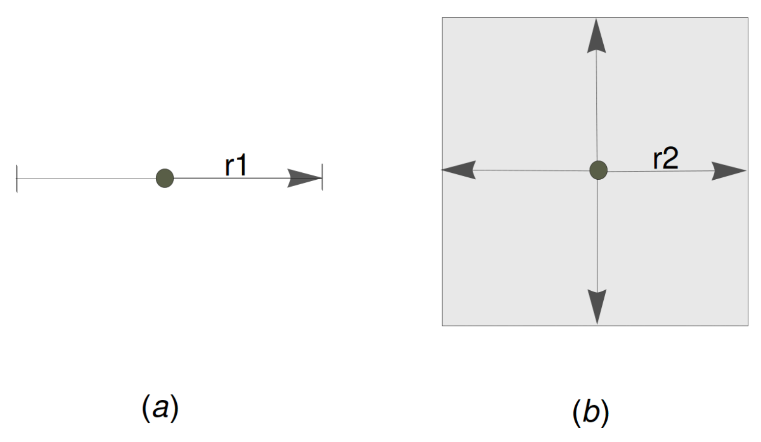
Fig. 1: (a) sensing radius $r_{1}$ on a line. (b) square sensing radius $r_{2}.$

However, in most cases the sensing area of a sensor is a circular disk of radius $r_{c}$ but our upper bound result proved in the sequel for square sensing radius $r_{2}$ are obviously valid for circular disk of radius $r_{c}$ equal to $\sqrt{2}r_{2}$ circumscribing the square.

The sensors are required to move from their current random locations to new positions so as to satisfy the following requirement.

Definition 3 ($(r_{m},s)$-C&I requirement).

Fix $m\in\{1,2\}.$ A set of sensors placed on the $m$-dimensional unit cube satisfy the $(r_{m},s)$ coverage & interference requirement if: requires:

1. Every point on the $m$-dimensional unit cube $[0,1]^{m}$ is within the range $r_{m}$ of a sensor, i.e. the $m$-dimensional unit cube is completely covered.

2. Each pair of sensors is placed at Euclidean distance greater or equal to $s.$

In this paper we investigate the problem of energy efficient displacement of the random mobile sensors.

Definition 4 (energy efficient displacement).

Assume that $n$ mobile sensors are placed independently and uniformly at random on the unit interval or on the unit square. The sensors move from their intial current location to the final destination so that in their final placement the sensor system satisfy the $(r_{m},s)$-coverage & interference requirement and the $a$-total displacement is minimized in expectation.

Throughout the paper, we will use the Landau asymptotic notations:

• $f(n)=O(g(n))$ if there exists a constant $C_{1}>0$ and integer $N$ such that $|f(n)|\leq C_{1}|g(n)|$ for all $n>N,$

• $f(n)=\Omega(g(n))$ if there exists a constant $C_{2}>0$ and integer $N$ such that $|f(n)|\geq C_{2}|g(n)|$ for all $n>N,$

• $f(n)=\Theta(g(n))$ if and only if $f(n)=O(g(n))$ and $f(n)=\Omega(g(n)),$

1.1 Contribution and Outline of the Paper

Let $a>0$ be a constant. Assume that $n$ mobile sensors with identical sensing radius $r_{1}$ and square sensing radius $r_{2}$ are placed independently at random with the uniform distribution on the unit interval and on the unit square.

In this paper we give the picture of the threshold phenomena for the coverage & interference requirement in one dimension, as well as in two dimension (see Definition 3). The $a$-total displacement (the energy consumption) is used to measure the movement cost (see Definition 1) while Euclidean distance is used for the interference distance and the sensing area of a sensor in two dimension is a square (see Definition 2). Let us also recall that in two dimension the sensors can move directly to the final locations via the shortest route not only in vertical and horizontal fashion.

Let $\epsilon>0$, $1>\delta>0$ be arbitrary small constants independent on the number of sensors $n.$

Table $1$ summarizes our main contribution in one dimension.

Table 1: The expected minimal $a$-total displacement of $n$ random sensors on the unit interval $[0,1]$ as a function of the sensing radius $r_{1}$ and the interference value $s,$ where $\epsilon>0$, $1>\delta>0.$

Sensing radius $r_{1}$	Interference distance $s$	Expected minimal $a$-total displacement for $(r_{1},s)-C\&I$ requirement	Theorem
$r_{1}=\frac{1}{2n}$	$s=\frac{1}{n}$	$\frac{\Gamma(\frac{a}{2}+1)}{2^{\frac{a}{2}}(1+a)}n^{1-\frac{a}{2}}+O\left(n^{-\frac{a}{2}}\right),$ $a>0$	10[cf. [15]]
$r_{1}=\frac{1+\epsilon}{2n},$ $\epsilon>0$	$s=\frac{1-\delta}{n},$ $1>\delta>0$	$O\left(n^{1-a}\right),\,\,$ $a>0$	16

As the sensing radius $r_{1}$ increases from $\frac{1}{2n}$ to $\frac{1+\epsilon}{2n}$ and the interference distance $s$ decreases from $\frac{1}{n}$ to $\frac{1-\delta}{n}$ there is a decline from $\Theta\left({n^{\frac{a}{2}}}n^{1-a}\right)$ to $O\left(n^{1-a}\right)$ in the expected minimal $a$-total displacement for all powers $a>0.$

Table $2$ summarizes our main contribution in two dimensions.

Table 2: The expected minimal $a$-total displacement of $n$ random sensors on the unit square $[0,1]^{2}$ as a function of the square sensing radius $r_{2}$ and the interference value $s,$ where $\epsilon>0$, $1>\delta>0.$

Square sensing radius $r_{2}$	Interference distance $s$	Expected minimal $a$-total displacement for $(r_{2},s)-C\&I$ requirement	Theorem
$r_{2}=\frac{1}{2\sqrt{n}}$	$s=\frac{1}{\sqrt{n}}$	$\Theta\left(\sqrt{\ln(n)n}\right)$   if   $a=1$ $\Omega\left((\ln(n))^{\frac{a}{2}}n^{1-\frac{a}{2}}\right)$   if   $a>1$	11[cf.[36]] 12
$r_{2}=\frac{1+\epsilon}{2\lfloor\sqrt{n}\rfloor},$ $\epsilon>0$	$s=\frac{1-\delta}{\lfloor\sqrt{n}\rfloor},$ $1>\delta>0$	$O\left(n^{1-\frac{a}{2}}\right)$  if   $a>0$	17

As the square sensing radius $r_{2}$ increases from $\frac{1}{2\sqrt{n}}$ to $\frac{1+\epsilon}{2\lfloor\sqrt{n}\rfloor}$ and the interference distance $s$ decreases from $\frac{1}{\sqrt{n}}$ to $\frac{1-\delta}{\lfloor\sqrt{n}\rfloor}$ There is a decline from $\Omega\left({{({\ln(n)})^{{\frac{a}{2}}}}}n^{1-\frac{a}{2}}\right)$ to $O\left(n^{1-\frac{a}{2}}\right)$ in the expected minimal $a$-total displacement for all powers $a\geq 1.$

Notice that $n$ sensors on the unit interval $[0,1]$ with sensing radius $r_{1}=\frac{1}{2n}$ and the interference distance have to move to the anchor positions to satisfy $\left(r_{1},s\right)$-coverage & interference. When $r_{1}>\frac{1}{2n}$ and $s<\frac{1}{n}$ there are no anchors positions predetermined in advance. The similar remark holds for the sensors on the unit square $[0,1]^{2}.$

Our theoretical results imply that the expected $a$-total displacement is constant and independent on number of sensors for some parameters $a.$ Namely, we have the following upper bounds:

• For the random sensors on the unit interval, when

  $$n(2r_{1})=1+\epsilon,$$

  i.e. the sum of sensing area of $n$ sensors is a little bigger then the length of the unit interval, it is possible to provide the full area coverage in $O(1)$ expected $a$-total displacement with $a\geq 1.$

• For the random sensors on the unit square, when

  $$n(2r_{2})^{2}\sim(1+\epsilon)^{2}\,\,\,\,\,\text{as}\,\,\,\,\,n\rightarrow\infty,$$

  i.e. the sum of sensing area of $n$ sensors is asymptotically a little bigger then the area of unit square, the expected $a$-total displacement with $a\geq 2$ to provide full area coverage is $O(1).$ Obviously, this result is easily applicable to the model when the sensing area of a sensor is a circular disk of radius $r_{c}$ by taking circle circumscribing the square. Namely, when

  $$n\pi(r_{c})^{2}\sim\frac{\pi}{2}(1+\epsilon)^{2}\,\,\,\,\,\text{as}\,\,\,\,\,n\rightarrow\infty$$

  then the expected $2$-total displacement to provide full area coverage is constant.

This constant cost seems to be of practical importance due to efficient monitoring against illegal trespassers. It is well known that intrusion detection is an important application of wireless sensor networks. In this case it is necessary to ensure coverage with good communication.

Notice that constant expected cost in (i) and (ii) are valid for $n$ random sensors with identical sensing radius $r_{1}=\frac{x(1+\epsilon)}{2n}$ on the interval of length $x$ and for $n$ random sensors with identical square sensing radius $r_{2}=\frac{x(1+\epsilon)}{2\lfloor\sqrt{n}\rfloor}$ on the square $[0,x]\times[0,x].$

We also present 3 algorithms (see Algorithms (1-3)). It is worthwhile to mention that, even though the algorithms are simple the analysis is challenging. Notice that Algorithms (1-3) can be implemented by a centralized controller telling each sensor where and when to move. In Section 2 we prove some technical properties of Beta distribution with special positive integer parameters needed in the current paper (see Lemma 6 and Lemma 7).

The overall organization of the paper is as follows. Subsection 1.2 briefly summarizes some related work. In Section 2 we present some preliminary results that will be used in the sequel. Sections 3 and 5 deals with sensors on the unit interval. In Sections 4 and 6 we investigate sensors on the unit square, while further insights in the higher dimension are discussed in Section 7. Section 8 deals with experimental evaluation of Algorithm 1. Section 9 contains conclusions and directions for future work. Finally, for the sake of readability, certain technical proofs are defarred to the Appendices.

1.2 Related Work

There are extensive studies dealing with both coverage (e.g., see [1, 3, 5, 35]) and interference problems (e.g., see [6, 9, 19, 29]). Closely related to barrier and area coverage the matching problem is also of interest in the research community (e.g., see [2, 16, 21, 36])

An important setting in considerations for coverage of a domain is when the sensors are initially placed at random with the uniform distribution. Some authors proposed using several rounds of random displacement to achieve complete coverage of a domain [12, 37]. Another approach is to have the sensors relocate from their initial position to a new position to achieve the desired coverage [7, 11].

More importantly, our work is closely related to the papers [26, 27] in respect to analysis of the expected $a$-total displacement for coverage problem where the sensors are randomly placed on the unit interval [27] and in the higher dimension [26]. Both papers study performance bounds for some algorithms, using Chernoff’s inequality. The methods used in these papers have limitations - the most important and difficult cases when the sensing radius $r_{1}$ is close to $\frac{1}{2n}$ and the square sensing radius $r_{2}$ is close to $\frac{1}{2\sqrt{n}}$ were not included in [26, 27]. Moreover, in the paper [26] the sensors can move only in parallel to the axes. Hence, the analysis of coverage problem in [26] is incomplete. Moreover, it is natural to investigate the general case when the sensor can move directly to the final locations via the shortest route not only in vertical and horizontal fashion. The novelty of work in the current paper lies in studying the cases for the threshold phenomena, when the sensing radius $r_{1}$ is close to $\frac{1}{2n},$ i.e. $r_{1}=\frac{1+\epsilon}{2n}$ and the square sensing radius $r_{2}$ is close to $\frac{1}{2\sqrt{n}},$ i.e. $r_{2}=\frac{1+\epsilon}{2\lfloor\sqrt{n}\rfloor}$ for coverage & interference, provided that $\epsilon$ is an arbitrary small constant independent on the number of sensors $n.$ Compared to the coverage problem, $(r_{m},s)-C\&I$ requirement not only ensures coverage, but also avoids interference and is more reasonable in order to provide reliable communication within the network.

Finally, it is worth mentioning that, our work is related to the series of papers [20, 22, 24, 8]. In [20, 22] the author investigated the maximum of the expected sensor’s displacement (the time required) for coverage & interference. In [20, 22] it is assumed that the $n$ sensors are initially deployed on the $[0,\infty)$ according to the arrival times of the Poisson process with arrival rate $\lambda>0$ and coverage (connectivity) is in the sense that there are no uncovered points from the origin to the last rightmost sensor. The work by [24] investigates the expected minimal $a$-total discplacement for interference-connectivity requirement when the $n$ sensors are initially placed on the $[0,\infty)^{d}$ according to $d$ identical and independent Poisson processes each with arrival rate $\lambda>0.$ It is worth pointing out that the $d$-dimensional model in [24] is only the direct extension of the interference-connectivity requirement from one dimension to the $d$-dimensional space and the sensors move only in parallel to the axes.

2 Preliminaries

In this section we introduce some basic concepts and notations that will be used in the sequel. We also present three lemmas which will be helpful in proving our main results. In this paper, in the one dimensional scenario, the $n$ mobile sensors are thrown independently at random following the uniform distribution in the unit interval $[0,1].$ Let $X_{(\ell)}$ be the position of the $\ell$-th sensor after sorting the initial random locations of $n$ sensors with respect to the origin of the interval $[0,1],$ i.e. the $\ell$-th order statistics of the uniform distribution in the unit interval. It is known that the random variable $X_{(\ell)}$ obeys the Beta distribution with parameters $\ell,n+1-\ell$ (see [4, page13]).

Assume that $c,d$ are positive integers. The Beta distribution $\mathrm{Beta}(c,d)$ (see [33]) with parameters $c,d$ is the continuous distribution on $[0,1]$ with probability density function $f_{c,d}(t)$ given by

$$f_{c,d}(t)=c\binom{c+d-1}{c}t^{c-1}(1-t)^{d-1},\,\,\,\text{when}\,\,\,0\leq t\leq 1.$$ (1)

The cumulative distribution function of the Beta distribution with parameters $c,d$ is given by the incomplete Beta function

$$I_{z}(c,d)=c\binom{c+d-1}{c}\int_{0}^{z}t^{c-1}(1-t)^{d-1}dt\,\,\,\text{for}\,\,\,0\leq z\leq 1.$$ (2)

Moreover, the incomplete Beta function is related to the binomial distribution by

$$1-I_{z}(c,d)=\sum_{j=0}^{c-1}\binom{c+d-1}{j}z^{j}(1-z)^{c+d-1-j}$$ (3)

(see [33, Identity 8.17.5] for $c:=m,$ $d:=n-m+1$ and $x:=z$) and the binomial identity

$$\sum_{j=0}^{c+d-1}\binom{c+d-1}{j}z^{j}(1-z)^{c+d-1-j}=1.$$ (4)

The following inequality which relates binomial and Poisson distribution was discovered by Yu. V. Prohorov (see [31, Theorem 2], [34]).

$$\binom{n}{j}x^{j}(1-x)^{n-j}\leq\left(\frac{n}{m_{1}}\right)^{\frac{1}{2}}e^{-nx}\frac{(nx)^{j}}{j!},$$ (5)

where $m_{1}$ is some integer which satisfies $n(1-x)-1<m_{1}\leq n(1-x).$

We will also use the classical Stirling’s approximation for factorial (see [13, page 54])

$$\sqrt{2\pi}N^{N+\frac{1}{2}}e^{-N+\frac{1}{12N+1}}<N!<\sqrt{2\pi}N^{N+\frac{1}{2}}e^{-N+\frac{1}{12N}}.$$ (6)

We use the following notation $|x|^{+}=\max\{x,0\}$ for the positive parts of $x\in\mathbb{R}.$

We are now ready to give some useful properties of Beta distribution in the following sequences of lemmas.

Lemma 5.

Let $a>0.$ Assume that $n$ is positive integer. Then

$$\Pr\left[\mathrm{Beta}(n,1)<1-\frac{1}{n^{\frac{a}{1+a}}}\right]<\frac{1}{e^{n^{\frac{1}{1+a}}}}.$$

Proof.

First of all observe that (see (1) for $c:=n$ and $d:=1.$)

$$\Pr\left[\mathrm{Beta}(n,1)<1-\frac{1}{n^{\frac{a}{1+a}}}\right] =\int_{0}^{1-\frac{1}{n^{\frac{a}{1+a}}}}f_{n,1}(t)dt=\left(1-\frac{1}{n^{\frac{a}{1+a}}}\right)^{n}$$

$$=\left(\left(1-\frac{1}{n^{\frac{a}{1+a}}}\right)^{n^{\frac{a}{a+1}}}\right)^{n^{\frac{1}{a+1}}}.$$ (7)

Using (2) and the basic inequality $(1-x)^{1/x}<e^{-1}$ when $x>0$ we have

$$\Pr\left[\mathrm{Beta}(n,1)<1-\frac{1}{n^{\frac{a}{1+a}}}\right]<\frac{1}{e^{n^{\frac{1}{1+a}}}}$$

which completes the proof. ∎

Lemma 6.

Let $a>0$ be a constant. Fix $\gamma>0$ independent on $n.$ Let $\rho=\frac{1+\gamma}{n}.$ Assume that $\ell,n$ are positive integers and $\ell\leq n.$ Then

$$\mathbb{E}\left[\left(|\mathrm{Beta}(\ell,n-\ell+1)-\rho\ell|^{+}\right)^{a}\right]=O\left(\frac{1}{n^{a}}\right),\,\,\,\text{uniformly in}\,\,\,\ell\in\{1,2,\dots,n\},$$ (8)

$$\sum_{\ell=1}^{n}\frac{n}{\ell}\mathbb{E}\left[\left(|\mathrm{Beta}(\ell,n-\ell+1)-\rho\ell|^{+}\right)^{a}\right]=O\left(n^{1-a}\right).$$ (9)

Proof.

The proof is given in Appendix A. ∎

Lemma 7.

Let $a>0$ be a constant. Fix $1>\delta>0$ independent on $n.$ Let $s=\frac{1-\delta}{n}.$ Assume that $\ell,n$ are positive integers and $\ell\leq n.$ Then

$$\sum_{\ell=1}^{n}\frac{n}{\ell}\mathbb{E}\left[\left(|s\ell-\mathrm{Beta}(\ell,n-\ell+1)|^{+}\right)^{a}\right]=O\left(n^{1-a}\right).$$ (10)

Proof.

The proof is given in Appendix B. ∎

The following lemma will simplify the upper bound estimations in Section 5 and Section 6.

Lemma 8.

Fix $a>0.$ Assume that the sensor movement $M$ is the finite sum of movements $M_{i}$ for $i=1,2,\dots,l,$ i.e. $M=\sum_{i=1}^{\ell}M_{i}.$ Then

$$\mathbb{E}[M^{a}]\leq C_{a,\ell}\sum_{i=1}^{\ell}\mathbb{E}[M_{i}^{a}],$$

where $C_{a,\ell}$ is some constant which depend only on fixed $a$ and $\ell.$

Proof.

Firstly we recall two elementary inequalities.

Fix $a\geq 1.$ Let $x,y\geq 0.$ Then

$$(x+y)^{a}\leq 2^{a-1}(x^{a}+y^{a}).$$ (11)

Notice that Inequality (11) is the consequence of the fact that $f(x)=x^{a}$ is convex over $\mathbf{R_{+}}$ for $a\geq 1.$

Fix $a\in(0,1).$ Let $x,y\geq 0.$ Then

$$(x+y)^{a}\leq x^{a}+y^{a}.$$ (12)

Combining together Inequality (11) and Inequality (12) for the sum $\sum_{i=1}^{\ell}M_{i}$ and passing to the expectations we derive

$$\mathbb{E}[M^{a}]\leq C_{a,\ell}\sum_{i=1}^{\ell}\mathbb{E}[M_{i}^{a}].$$

This proves Lemma 8. ∎

3 Coverage & interference requirement when the sensing radius $r_{1}=\frac{1}{2n}$ and the interference distance $s=\frac{1}{n}$

In this section, we recall the known results about the expected $a$-total displacement to fulfill the $(r_{1},s)-C\&I$ requirement when $n$ mobile sensors with identical sensing radius $r_{1}=\frac{1}{2n}$ are distributed uniformly at random and independently on the unit interval $[0,1].$ That is, the sum of sensing area of $n$ sensors is equal to the length of the unit interval. Observe that in the case when the sensing radius $r_{1}=\frac{1}{2n}$ and the interference distance $s=\frac{1}{n}$ the only way to achieve $\left(r_{1},s\right)$-coverage & interference requirement on the unit interval $[0,1]$ is for the sensors to occupy the equidistant anchor positions $\frac{i}{n}-\frac{1}{2n}$, for $i=1,2,\ldots,n.$ The following exact asymptotic result was proved in [27].

Theorem 9 ([27]).

Let $a$ be an even positive natural number. Assume that, $n$ mobile sensors are thrown uniformly and independently at random on the unit interval $[0,1].$ The expected $a$-total displacement of all $n$ sensors, when the $i$-th sensor sorted in increasing order moves from its current random location to the equidistant anchor location $\frac{i}{n}-\frac{1}{2n}$, for $i=1,2,\ldots,n$, respectively, is $\frac{\left(\frac{a}{2}\right)!}{2^{\frac{a}{2}}(1+a)}n^{1-\frac{a}{2}}+O\left(n^{-\frac{a}{2}}\right).$

In [15], Theorem 9 was extended to all real valued exponents $a>0.$

Theorem 10 ([15]).

Fix $a>0.$ Assume that, $n$ mobile sensors are thrown uniformly and independently at random on the unit interval $[0,1].$ The expected $a$-total displacement of all $n$ sensors, when the $i$-th sensor sorted in increasing order moves from its current random location to the equidistant anchor location $\frac{i}{n}-\frac{1}{2n}$, for $i=1,2,\ldots,n$, respectively, is

$$\frac{\Gamma\left(\frac{a}{2}+1\right)}{2^{\frac{a}{2}}(1+a)}n^{1-\frac{a}{2}}+O\left(n^{-\frac{a}{2}}\right).$$ (13)

The gamma function $\Gamma(a)$ is defined to be an extension of the factorial to real number arguments. It is related to the factorial by $\Gamma\left(\frac{a}{2}+1\right)=\left(\frac{a}{2}\right)!$ provided that $\frac{a}{2}\in{\mathbb{N}}.$ It is also worthwhile to mention that, the extension of direct combinatorial method from [27] leads to exact asymptotic result in Theorem 10 only when $a$ is an odd natural number (see [23, Theorem 2]).

4 Coverage & interference requirement when the square sensing radius $r_{2}=\frac{1}{2\sqrt{n}}$ and the interference distance $s=\frac{1}{\sqrt{n}}$

In this section, we analyze the expected $a$-total displacement to achieve $(r_{2},s)-C\&I$ requiremnt when $n$ mobile sensors with identical square sensing radius $r_{2}=\frac{1}{2\sqrt{n}}$ are thrown uniformly at random and independently on the unit square $[0,1]^{2},$ provided that $n$ is the square of a natural number. That is, the sum of sensing area of $n$ sensors is equal to the area of unit square.

Observe that to fulfill $\left(\frac{1}{\sqrt{n}},\frac{1}{2\sqrt{n}}\right)$-coverage & interference requirement the sensors have to occupy the following anchor positions $\left(\frac{k}{\sqrt{n}}-\frac{1}{2\sqrt{n}},\frac{l}{\sqrt{n}}-\frac{1}{2\sqrt{n}}\right),$ where $1\leq k,l\leq\sqrt{n}$ and $n$ must be the square of a natural number.

It is known that expected $1$-total displacement in this case is $\Theta\left(\sqrt{\ln(n)n}\right).$ Namely, the following theorem about the optimal transportation cost for random matching was obtained in [36] a book related to these problems which develops modern methods to bound stochastic processes.

Theorem 11 ([36], Chapter 4.3).

Let $n=q^{2}$ for some $q\in\mathbb{N}.$ Assume that $n$ mobile sensors $X_{1},X_{2},\dots,X_{n}$ are thrown uniformly and independently at random on the unit square $[0,1]^{2}.$ Consider the non-random points $(Z_{i})_{i\leq n}$ evenly distributed as follows: $Z_{i}=\left(\frac{k}{\sqrt{n}}-\frac{1}{2\sqrt{n}},\frac{l}{\sqrt{n}}-\frac{1}{2\sqrt{n}}\right),$ where $1\leq k,l\leq\sqrt{n},\,\,$ $i=k\sqrt{n}+l.$ Then

$$\mathbb{E}\left({\min_{\pi}\sum_{i=1}^{n}d\left(X_{i},Z_{\pi(i)}\right)}\right)=\Theta\left(\sqrt{\ln(n)n}\right),$$

where the infimum is over all permutations of $\{1,2,\dots,n\}$ and where $d$ is the Euclidean distance.

We are now ready to extend Theorem 11 to the displacement to the power $a$ provided that $a>1.$

Theorem 12.

Fix $a>1.$ Let $n=q^{2}$ for some $q\in\mathbb{N}.$ Assume that $n$ mobile sensors $X_{1},X_{2},\dots,X_{n}$ are thrown uniformly and independently at random on the unit square $[0,1]^{2}.$ Consider the non-random points $(Z_{i})_{i\leq n}$ evenly distributed as follows:
$Z_{i}=\left(\frac{k}{\sqrt{n}}-\frac{1}{2\sqrt{n}},\frac{l}{\sqrt{n}}-\frac{1}{2\sqrt{n}}\right),$ where $1\leq k,l\leq\sqrt{n},\,\,$ $i=k\sqrt{n}+l.$ Then

$$\mathbb{E}\left({\min_{\pi}\sum_{i=1}^{n}d^{a}\left(X_{i},Z_{\pi(i)}\right)}\right)=\Omega\left((\ln(n))^{\frac{a}{2}}n^{1-\frac{a}{2}}\right),$$

where the infimum is over all permutations of $\{1,2,\dots,n\}$ and where $d$ is the Euclidean distance.

Proof.

(Theorem 12) Let $\pi^{\star}\in S_{n}$ be a permutation with

$$T^{(b)}=\sum_{i=1}^{n}d^{b}\left(X_{i},Z_{\pi^{\star}(i)}\right)=\inf_{\pi\in S_{n}}\sum_{i=1}^{n}d^{b}\left(X_{i},Z_{\pi(i)}\right),\,\,\,1\leq b<\infty$$

where $S_{n}$ is the set of all permutations of the numbers $1,2,\dots,n.$
Fix $a>1.$ Applying discrete Hölder inequality we get

$$\sum_{i=1}^{n}d\left(X_{i},Z_{\pi^{\star}(i)}\right)\leq\left(\sum_{i=1}^{n}d^{a}\left(X_{i},Z_{\pi^{\star}(i)}\right)\right)^{\frac{1}{a}}\left(\sum_{i=1}^{n}1\right)^{\frac{a-1}{a}}.$$

Hence

$$\left(T^{(1)}\right)^{a}\leq T^{(a)}n^{a-1}.$$

Passing to the expectations and using Jensen inequality for $X:=T^{(1)}$ and $f(x)=x^{a}$ we get the following estimation

$$\left(\mathbb{E}\left({T^{(1)}}\right)\right)^{a}\leq\mathbb{E}\left({T^{(a)}}n^{a-1}\right).$$ (14)

Putting together Theorem 11 and inequality (14) we obtain

$$\mathbb{E}\left({T^{(a)}}\right)\geq n^{1-a}\left(\Theta\left(\sqrt{\ln(n)n}\right)\right)^{a}=\Theta\left((\ln(n))^{\frac{a}{2}}n^{1-\frac{a}{2}}\right).$$

Therefore

$$\mathbb{E}\left({\inf_{\pi}\sum_{i=1}^{n}d^{a}\left(X_{i},Z_{\pi(i)}\right)}\right)=\Omega\left((\ln(n))^{\frac{a}{2}}n^{1-\frac{a}{2}}\right).$$

This completes the proof of Theorem 12. ∎

5 Coverage & interference requirement when the sensing radius $r_{1}>\frac{1}{2n}$ and the interference distance $s<\frac{1}{n}.$

In this section, we analyze the expected $a$-total displacement to fulfill $(r_{1},s)-C\&I$ requirement when $n$ mobile sensors with identical sensing radius $r_{1}>\frac{1}{2n}$ are distributed uniformly at random and independently on the unit interval $[0,1].$ That is, the sum of sensing area of $n$ sensors is greater than the length of the unit interval.

5.1 Analysis of Algorithm 1

Algorithm 1 $MV(n,\rho,s)$ Moving sensors on $[0,1].$

0:  The initial locations of $n$ mobile sensors, placed uniformly and independently at random on the unit interval $[0,1].$

0:  The final positions of the sensors such that:

1. The distance between consecutive sensors is greater than or equal to $s$ and less than or equal to $\rho.$

2. The leftmost sensor is at a distance less than or equal to $\frac{\rho}{2}$ from the origin.

Initialization:   Sort the initial locations of $n$ sensors with respect to the origin of the interval, the location and sensors after sorting $X_{(1)}\leq X_{(2)}\leq\dots\leq X_{(n)};$

1:  Let $X_{0}=0;$

2:  for $i=1$ to $n$  do

3:     if $X_{(i)}-X_{(i-1)}<s$ then

4:        move left to right the sensor $X_{(i)}$ to the new position $\min\left(s+X_{(i-1)},1\right);$

5:     else if $X_{(i)}-X_{(i-1)}>\rho$ then

6:        move right to left the sensor $X_{(i)}$ to the new position $\rho+X_{(i-1)};$

7:     else

8:        do nothing;

9:     end if

10:  end for

11:  if $X_{(1)}>\frac{1}{2}\rho$ then

12:     $z:=X_{(1)}-\frac{1}{2}\rho;$

13:     for $i=1$ to $n$  do

14:        move right to left the sensor $X_{(i)}$ to the new position $X_{(i)}-z;$

15:     end for

16:  end if

Fix $a>0.$ Let $\gamma>0$, $1>\delta>0$ be arbitrary small constants independent on the number of sensors $n$ and let $\rho=\frac{1+\gamma}{n},\,\,$ $s=\frac{1-\delta}{n}.$

This subsection is concerned with reallocating of the $n$ random sensors within the unit interval to achieve only the following property:

• The distance between consecutive sensors is greater than or equal to $s$ and less than or equal to $\rho.$

• The first leftmost sensor is at a distance less than or equal to $\frac{\rho}{2}$ from the origin.

We present basic and energy efficient algorithm $MV(n,\rho,s)$ (see Algorithm 1). Theorem 13 states that the expected $a$-total displacement of algorithm $MV(n,\rho,s)$ is in $O\left(n^{1-a}\right)$ when $\rho=\frac{1+\gamma}{n}$ and $s=\frac{1-\delta}{n}.$ Algorithm 1 is very simple but the asymptotic analysis is not totally trivial. We note that asymptotic analysis of Algorithm 1 is crucial in deriving the threshold phenomena.

In the proof of Theorem 13 we combine combinatorial techniques with properties of the Beta distribution (see Equation (9) in Lemma 6 and Equation (10) in Lemma 7). The estimations for Beta distribution with special positive integers parameters in Lemma 6 and Lemma 7 are new to the best of the author’s knowledge.

Before starting the proof of Theorem 13, we briefly discuss one technical issue in the steps $(3)$-$(4)$ of Algorithm 1. It may happen that for some initial random location of $n$ sensors $X_{(1)}\leq X_{(2)}\leq\dots\leq X_{(n)}$ Algorithm 1 moves some sensors to the right endpoint of the interval $[0,1].$ Namely, there exists $l_{0}\in\mathbb{N_{+}}$ with the following property $X_{(i)}$ moves to some point in $[0,1)$ for all $i=1,2,\dots,l_{0}$ and $X_{(i)}$ moves to the right endpoint of the interval $[0,1]$ for all $i=l_{0}+1,l_{0}+2,\dots,n.$ Let $Y_{1},Y_{2},\dots,Y_{n}$ be the location of $n$ sensors $X_{(1)}\leq X_{(2)}\leq\dots\leq X_{(n)}$ after Algorithm 1. Then to avoid interference to achieve the property that the distance between consecutive sensors is greater than or equal to $s$, we have to deactivate some sensors. Namely,

• if $1-Y_{l_{0}}<s$ then for all $i=l_{0}+1,l_{0}+2,\dots,n$ the sensors $X_{(i)}$ will not sense any longer,

• if $1-Y_{l_{0}}\geq s$ then for all $i=l_{0}+2,l_{0}+3,\dots,n$ the sensors $X_{(i)}$ will not sense any longer.

We are now ready to give the proof of Theorem 13.

Theorem 13.

Let $a>0$ be a constant. Fix $\gamma>0$, $1>\delta>0$ independent on the number of sensors $n.$ Assume that $n$ mobile sensors are thrown uniformly and independently at random on the unit interval $[0,1].$ Then Algorithm 1 for $\rho=\frac{1+\gamma}{n}$ and $s=\frac{1-\delta}{n}$ reallocates the random sensors within the unit interval so that:

• The distance between consecutive sensors is greater than or equal to $s$ and less than or equal to $\rho.$

• The leftmost sensor is at a distance less than or equal to $\frac{\rho}{2}$ from the origin.

• The expected $a$-total displacement is $O\left(n^{1-a}\right).$

Notice that Theorem 13 is valid regardless of the sensing radius, it depends only on the fact that the relocated sensors are not too far.

Proof.

Let $\rho=\frac{1+\gamma}{n}$ and $s=\frac{1-\delta}{n},$ provided that $\gamma>0$, $1>\delta>0$ are arbitrary small constants independent on the number of sensors $n.$ Notice that Algorithm (1) is in two phases. During the first phase (see steps ($(1)$-$(10)$)) we reallocate the sensors so that the distance between consecutive sensors is greater than or equal to $s$ and less than or equal to $\rho.$ In the second phase (see steps ($(11)$-$(16)$)) we reallocate the sensors to achieve the additional property the first leftmost sensor is in the distance less than or equal to $\frac{\rho}{2}$ from the origin.

Hence the properties (i) and (ii) hold and thus Algorithm 1 is correct.

We now estimate the expected $a$-total displacement of the algorithm.

First Phase      The steps $(1)$-$(10)$ of Algorithm 1
The main idea of the proof is simple. Algorithm 1 produces a sequence of moves for $X_{(i)}$ which consists of left moves (say $L$), right moves (say $R$) or no move at all (say $U$). Now, the idea of the proof is to chop the resulting set of moves into a run of $L$ followed by a run of $R$ followed by a run of $U$, etc. (Here runs might be empty as well.) Using this, we give an upper bound on the total displacement (namely the bound (16)) whose expectation is then bounded.
Notice that exist $i\in\{1,2,\dots,n\}$ such that Algorithm 1 leaves the sensors $X_{(1)},X_{(2)},\dots$ $X_{(i-1)}$ at the same positions. (Here for $i=1$ Algorithm moves the sensor $X_{1}$) Then the steps ($(1)$-$(10)$) of Algorithm 1 are the sequence of the two phases: $A$ and $B.$ During phase $A,$ Algorithm 1 moves the sensors $X_{(i+1)},X_{(i+2)},$ $\dots X_{(i+p)}$ at the new positions. $k\in\{1,2,\dots,n\}.$ Then in phase $B,$ Algorithm 1 leaves the sensors $X_{(i+p+1)},X_{(i+p+2)},$ $\dots X_{(i+p+k)}$ at the same positions. (Here phase $B$ might not exist and Algorithm 1 moves the sensors $X_{(i+1)},X_{(i+2)},$ $\dots X_{(n)}$).

To better illustrate analysis, let us consider the following example. Consider the phase $A$ as specified above. Let $p=p_{1}+p_{2}$ for some $p_{1},p_{2}\in\mathbb{N_{+}}.$

1. The sensors $X_{(i+1)},X_{(i+2)},\dots X_{(i+p_{1})}$ move right to left. Observe that the sensors $X_{(i+1)},X_{(i+2)},\dots X_{(i+p_{1})}$ have to move cumulatively, namely for $\ell=1,2,\dots,p_{1}$ the sensor $X_{(i+\ell)}$ moves right to left to the position $X_{(i)}+\rho\ell.$ The displacement to the power $a$ is

   $$T^{a}_{1}=\sum_{\ell=1}^{p_{1}}\left(\left|X_{(i+\ell)}-X_{(i)}-\rho\ell\right|^{+}\right)^{a}.$$

2. The sensors $X_{(i+p_{1}+1)},X_{(i+p_{1}+2)},\dots X_{(i+p_{1}+p_{2})}$ move left to right. Notice that the sensors $X_{(i+p_{1}+1)},X_{(i+p_{1}+2)},\dots X_{(i+p_{1}+p_{2})}$ have to move cumulatively, namely for $\ell=1,2,\dots,p_{2}$ the sensors $X_{(i+p_{1}+\ell)}$ move left to right to the position $X_{(i)}+\rho p_{1}+s\ell.$ The displacement to the power $a$ is
   $T^{a}_{2}=\sum_{\ell=1}^{p_{2}}\left(\left|X_{(i)}+\rho p_{1}+s\ell-X_{(i+p_{1}+\ell)}\right|^{+}\right)^{a}.$ Since $X_{(i)}+\rho p_{1}<X_{(i+p_{1})}$ (see Figure 2) we upper bound the displacement to the power $a$ as follows:

   $$T^{a}_{2}\leq\sum_{\ell=1}^{p_{2}}\left(\left|X_{(i+p_{1})}+s\ell-X_{(i+p_{1}+\ell)}\right|^{+}\right)^{a}.$$

Fig. 2: The movement of mobile sensors $X_{(i+p_{1})},$ $X_{(i+p_{1}+\ell)}$ specified by $1.$ and $2.$ in the phase $A$ of Algorithm 1.

We are now ready to estimate the movement of sensors in the phase $A$ in Algorithm 1. Let $p=p_{1}+p_{2}+\dots p_{m}$ for some $p_{1},p_{2},\dots p_{m}\in\mathbb{N_{+}}$ and $p_{0}=0.$ We assume that phase $A$ is divided into $m$ subphases as follows. Algorithm 1 moves cumulatively the sensors $X_{(i+p_{1}+p_{2}+\dots p_{j-1}+1)},$ $X_{(i+p_{1}+p_{2}+\dots p_{j-1}+2)},\dots,$
$X_{(i+p_{1}+p_{2}+\dots p_{j-1}+p_{j})}$ into one chosen direction left to right or right to left. The movement direction of the sensors $X_{(i+p_{1}+p_{2}+\dots p_{j-1}+1)},$ $X_{(i+p_{1}+p_{2}+\dots p_{j-1}+2)},\dots,$ $X_{(i+p_{1}+p_{2}+\dots p_{j-1}+p_{j})}$ is opposite to the movement direction of the sensors
$X_{(i+p_{1}+p_{2}+\dots p_{j}+1)},$ $X_{(i+p_{1}+p_{2}+\dots p_{j}+2)},\dots,$ $X_{(i+p_{1}+p_{2}+\dots p_{j}+p_{j+1})},$ provided that $j=1,2,\dots,m-1.$

Let $T^{a}_{p}$ be the displacement to the power $a$ in the considered phase $A$ of Algorithm 1 and let $p_{0}=0.$ Observe that

$$T^{a}_{p} \leq\max_{0<p_{1}+\dots+p_{m}\leq p}\sum_{j=1}^{m}\sum_{\ell=1}^{p_{j}}\left(|X_{(i+p_{1}+\dots+p_{j-1}+\ell)}-X_{(i+p_{1}+\dots+p_{j-1})}-\rho\ell|^{+}\right)^{a}$$

$$+\max_{0<p_{1}+\dots+p_{m}\leq p}\sum_{j=1}^{m}\sum_{\ell=1}^{p_{j}}\left(|X_{(i+p_{1}+\dots+p_{j-1})}+s\ell-X_{(i+p_{1}+\dots+p_{j-1}+\ell)}|^{+}\right)^{a}.$$ (15)

Let $T^{a}$ be the displacement to the power $a$ of Algorithm 1 in steps $(1)$-$(10)$ . Using (15), as well as the observation that Algorithm 1 is the sequence of the two phases $A$ and $B$ we get the following upper bound

$$T^{a}_{p}\leq$$

$$\max_{0\leq p_{1}+\dots+p_{m}\leq p,\,\,\,1\leq p\leq n}\sum_{j=1}^{m}\sum_{\ell=1}^{p_{j}}\left(|X_{(i+p_{1}+\dots+p_{j-1}+\ell)}-X_{(i+p_{1}+\dots+p_{j-1})}-\rho\ell|^{+}\right)^{a}$$

$$+\max_{0\leq p_{1}+\dots+p_{m}\leq p,\,\,\,1\leq p\leq n}\sum_{j=1}^{m}\sum_{\ell=1}^{p_{j}}\left(|X_{(i+p_{1}+\dots+p_{j-1})}+s\ell-X_{(i+p_{1}+\dots+p_{j-1}+\ell)}|^{+}\right)^{a}.$$ (16)

Let $b_{1,\ell},b_{2,\ell}$ be some integers such that $b_{1,\ell},b_{2,\ell}\in\{1,2,\dots,n\}$ and $b_{1,l}-b_{2,l}=\ell.$ Observe that the following costs $\left(|X_{(b_{1,\ell})}-X_{(b_{2,\ell})}-\rho\ell|^{+}\right)^{a}$
and $\left(|X_{(b_{2,\ell})}+sl-X_{(b_{1,\ell})}|^{+}\right)^{a}$ can appear in the double sums (16) at most $\frac{n}{\ell}$ times. Hence

$$T^{a}\leq\sum_{\ell=1}^{n}\frac{n}{\ell}\left(|X_{(b_{1,\ell})}-X_{(b_{2,\ell})}-\rho\ell|^{+}\right)^{a}+\sum_{\ell=1}^{n}\frac{n}{\ell}\left(|s\ell-X_{(b_{1,l})}-X_{(b_{2,l})}|^{+}\right)^{a}.$$ (17)

Let as recall the following claim.

Claim 14.

The random variable

$$X_{(j+\ell)}-X_{(j)}\,\,\,\text{has the}\,\,\,\mathrm{Beta}(\ell,n-\ell+1)\,\,\,\text{distribution}$$ (18)

(see [4, Formula 2.5.21, page 33]).

Combining (17), (18) we have for the expectation value

$$\mathbb{E}\left(T^{a}\right) \leq\sum_{l=1}^{n}\frac{n}{l}\mathbb{E}\left(|\mathrm{Beta}(\ell,n-\ell+1)-\rho l|^{+}\right)^{a}$$

$$+\sum_{l=1}^{n}\frac{n}{l}\mathbb{E}\left(|sl-\mathrm{Beta}(\ell,n-\ell+1)|^{+}\right)^{a}.$$

Combining Equation (9) in Lemma 6 and Equation (10) in Lemma 7 lead to $\mathbb{E}\left(T^{a}\right)=O\left(n^{1-a}\right).$ This is enough to prove the desired upper bound in the First Phase.

Second Phase      The steps $(11)$-$(16)$ of Algorithm 1

Observe that, after the steps $(1)$-$(10)$ the sensor $X_{(1)}$ has to be at position $P_{1}$ such that $0\leq P_{1}\leq\rho=\frac{1+\gamma}{n}.$ Hence for each sensor we upper bound the movement to the power $a$ by $\left(\frac{\rho}{2}\right)^{a}.$ Therefore, the expected $a$-total displacement of Algorithm 1 is less than

$$\sum_{i=1}^{n}\left(\frac{\rho}{2}\right)^{a}=\frac{(1+\gamma)^{a}}{2^{a}}n^{1-a}=O\left(n^{1-a}\right).$$

This is enough to prove the desired upper bound in the second case.
Finally, combining together the estimation from both phases and Lemma 8 completes the proof of Theorem 13. ∎

Finally, the following lemma will be helpful in the proof of the main results in Subsection 5.2 for the sensors on the unit interval. In the proof of Lemma 15 we combine probabilistic techniques together with Estimation (8) in Lemma 6 for Beta distribution from Section 2.

Lemma 15.

Let $a>0$ be a constant. Fix $\gamma>0$, $1>\delta>0$ independent on the number of sensors $n.$ Let $\rho=\frac{1+\gamma}{n}$ and $s=\frac{1-\delta}{n}.$ Let $Y_{n}$ be the location of $n$-th sensor after algorithm $MV(n,\rho,s).$ Then

$$\Pr\left[Y_{n}<1-\frac{2}{n^{\frac{a}{a+1}}}\right]=O\left(\frac{1}{n^{\frac{a}{2}}}\right).$$

Proof.

Let $M_{n}(1-10)$ be the movement of sensor $X_{(n)}$ right to left in Algorithm 1 at steps $(1)$-$(10).$ The analysis of $M_{n}(1-10)$ is analogous to that in the proof of Theorem 13. Using Equation (8) in Lemma 6 for ${\frac{(a+1)a}{2}}$ we get

$$\mathbb{E}\left[\left(M_{n}(1-10)\right)^{\frac{(a+1)a}{2}}\right]=O\left(\frac{1}{n^{\frac{(a+1)a}{2}}}\right).$$ (19)

Let $M_{n}(11-16)$ be the movement of sensor $X_{(n)}$ right to left in Algorithm 1 at the steps $(11)$-$(16).$ Observe that $M_{n}(11-16)\leq\frac{\rho}{2}=\frac{1}{2}\frac{1+\gamma}{n}.$ Therefore

$$\mathbb{E}\left[\left(M_{n}(11-16)\right)^{\frac{(a+1)a}{2}}\right]=O\left(\frac{1}{n^{\frac{(a+1)a}{2}}}\right).$$ (20)

Let $M_{n}$ be the movement of sensor $X_{(n)}$ right to left in Algorithm 1. Putting together the equality $M_{n}=M_{n}(1-10)+M_{n}(11-16),$ Estimations (19-20), as well as Lemma 8 we have

$$\mathbb{E}\left[\left(M_{n}\right)^{\frac{(a+1)a}{2}}\right]=O\left(\frac{1}{n^{\frac{(a+1)a}{2}}}\right).$$ (21)

Applying Markov inequality applied for random variable $M_{n}^{\frac{(a+1)a}{2}}$ and Estimation (21) we deduce that

$$\Pr\left[M_{n}>\frac{1}{n^{\frac{a}{1+a}}}\right]=\Pr\left[\left(M_{n}\right)^{\frac{(a+1)a}{2}}>\frac{1}{n^{\frac{a^{2}}{2}}}\right]=O\left(\frac{n^{\frac{a^{2}}{2}}}{n^{\frac{(a+1)a}{2}}}\right)=O\left(\frac{1}{n^{\frac{a}{2}}}\right).$$ (22)

Consider the following three events:

$$E_{1}:Y_{n}<1-2n^{-\frac{a}{a+1}}\,\,|\,\,X_{(n)}\geq 1-n^{-\frac{a}{a+1}},$$

$$E_{2}:Y_{n}<1-2n^{-\frac{a}{a+1}}\,\,|\,\,X_{(n)}<1-n^{-\frac{a}{a+1}},$$

$$E_{3}:X_{(n)}<1-n^{-\frac{a}{a+1}}.$$

Applying Equation (22) yields

$$\Pr\left[E_{1}\right]\left(1-\Pr\left[E_{3}\right]\right)\leq\Pr\left[E_{1}\right]\leq\Pr\left[M_{n}>\frac{1}{n^{\frac{a}{a+1}}}\right]=O\left(\frac{1}{n^{\frac{a}{2}}}\right).$$

From Lemma 5, as well as the fact that random $X_{(n)}$ obeys $\mathrm{Beta}(n,1)$ we have

$$\Pr\left[E_{2}\right]\Pr\left[E_{3}\right]\leq\Pr\left[E_{3}\right]<\frac{1}{e^{n^{\frac{1}{1+a}}}}\,\,\,\,\,\,\text{is exponentially small.}$$

Putting all together we deduce that

$$\Pr\left[Y_{n}<1-\frac{2}{n^{\frac{a}{a+1}}}\right]=\Pr\left[E_{1}\right]\left(1-\Pr\left[E_{3}\right]\right)+\Pr\left[E_{2}\right]\Pr\left[E_{3}\right]=O\left(\frac{1}{n^{\frac{a}{2}}}\right).$$

This finishes the proof of Lemma 15. ∎

5.2 Analysis of Algorithm 2

Let us recall that $a>0$ is fixed and $\epsilon>0$, $1>\delta>0$ are arbitrary small constants independent on the number of sensors $n.$ In this subsection we present algorithm $CV_{1}(n,r_{1},s)$ (see Algorithm 2) for the $(r_{1},s)-C\&I$ requirement. We prove that the expected $a$-total displacement of algorithm $CV_{1}(n,r,s)$ is in $O\left(n^{1-a}\right)$ when $r_{1}=\frac{1+\epsilon}{2n}$ and $s=\frac{1-\delta}{n}.$ Notice that our Algorithm 2 consists of two phases. During the first phase (see Initialization) we apply Algorithm 1. Then in the second phase (see Case B and Case C) we add the additional sensors movement. Let $Y_{n}$ be the location of sensors $X_{(n)}$ after Algorithm 2. The additional movement depends on the position of sensor $Y_{n}$ in the interval $[0,1].$

Algorithm 2 $CV_{1}(n,r_{1},s)$ for $(r_{1},s)$-coverage & interference requirement on $[0,1]$ when $r_{1}=\frac{1+\epsilon}{2n},\,\,\,$ $s=\frac{1-\delta}{n}$ provided that $\epsilon>0$, $1>\delta>0$ are fixed and independent on $n.$

0:  The initial locations of $n$ mobile sensors with identical sensing radius $r_{1}=\frac{1+\epsilon}{2n}$, placed uniformly and independently at random on the unit interval $[0,1].$

0:  The final positions of sensors to satisfy $(r_{1},s)$-coverage & interference requirement on the interval $[0,1].$ Initialization:   Apply Algorithm $MV(n,\rho,s)$ for $\rho:=\frac{1+\frac{\epsilon}{2}}{n},\,\,\,$ $s:=\frac{1-\delta}{n}$ and the random sensors $X_{1},X_{2},\dots,X_{n}.$ Let $Y_{1},Y_{2},\dots,Y_{n}$ be the location and sensors of $n$ sensors $X_{(1)}\leq X_{(2)}\leq\dots\leq X_{(n)}$ after Algorithm $MV(n,\rho,s);$

1:  switch ()

2:  case A $\left(Y_{n}\geq 1-r_{1}\right)$

3:     do nothing;

4:  case B $\left(Y_{n}\leq 1-\frac{2}{n^{\frac{a}{a+1}}}\right)$

5:     for $i=1$ to $n$  do

6:        move the sensor $Y_{i}$ to the position $\left(\frac{i}{n}-\frac{1}{2n}\right);$

7:     end for

8:  case C $\left(Y_{n}\in\left(1-\frac{2}{n^{\frac{a}{a+1}}},1-r_{1}\right)\right)$

9:     move the sensor $Y_{n}$ to the new position $1-r_{1},\,\,\,$ $i:=n-1;$

10:     while $Y_{i+1}-Y_{i}>2r_{1}$ do

11:        move the sensor $Y_{i}$ to the new position $1-r_{1}-(n-i)2r_{1},\,\,\,$ $i:=i-1$;

12:     end while

13:  end switch

We now briefly explain the ideas behind the proof of Theorem 16 and correctness of Algorithm 2.

• We have initially $n$ random sensors on the unit interval with identical sensing radius $r_{1}=\frac{1+\epsilon}{2n}.$ Firstly, we apply Algorithm 1 for $\rho=\frac{1+\frac{\epsilon}{2}}{n}$ and $s=\frac{1-\delta}{n}$ to achieve only the following property:

  • The distance between consecutive sensors is greater than or equal to $\frac{1-\delta}{n}$ and less than or equal to $\frac{1+\frac{\epsilon}{2}}{n}.$

  • The first leftmost sensor is at a distance less than or equal to $\frac{1+\frac{\epsilon}{2}}{2n}$ from the origin.

  Applying Theorem 13 we deduce that the expected $a$-total displacement in Initialization of Algorithm 2 is $O\left(n^{1-a}\right).$

• In case B we move the sensors to equidistant anchor locations in $\Theta\left(n^{1-\frac{a}{2}}\right)$ expected $a$-total displacement. However, we can upper bound the probability with which case B occurs (see Lemma 15) to achieve the desired $O\left(n^{1-a}\right)$ expected $a$-total displacement.

• Since the sensors have sensing radius $r_{1}=\frac{1+\epsilon}{2n}$ and the distance between consecutive sensors is less than or equal to $\frac{1+\frac{\epsilon}{2}}{n}=2r_{1}-\frac{\frac{\epsilon}{2}}{n},$ $(r_{1},s)$-coverage & interference requirement is solved in $O\left(n^{1-a}\right)$ expected $a$-total displacement in case C of Algorithm 2. In this case only fraction $\Theta\left(n^{\frac{1}{a+1}}\right)$ of rightmost sensors can move. We upper bound the movement to the power $a$ of each these sensors by $\frac{2^{a}}{n^{\frac{a^{2}}{a+1}}}$ (see Case 3 in the proof of Theorem 16).

We are now ready to prove the main theorem for the sensors on the unit interval.

Theorem 16.

Let $a>0$ be a constant. Fix $\epsilon>0$, $1>\delta>0$ independent on the number of sensors $n.$ Let $s=\frac{1-\delta}{n}.$ Assume that $n$ mobile sensors with identical sensing radius $r_{1}=\frac{1+\epsilon}{2n}$ are thrown uniformly and independently at random on the unit interval $[0,1].$ Then Algorithm 2 solves $(r_{1},s)$-coverage & interference requirement and has expected $a$-total displacement $O\left(n^{1-a}\right).$

Proof.

There are three cases to consider.

Case $1$: The algorithm terminates after Step $3$. This case adds nothing to the expected $a$-total displacement.

Case $2$: The algorithm terminates after Step $7$. Then $Y_{n}\leq 1-\frac{2}{n^{\frac{a}{a+1}}}.$

In this case we upper bound the expected $a$-total displacement in steps $(5)$-$(7)$ of algorithm $CV_{1}(n,r_{1},s)$ as follows:

• rewind the $i$-th sensor from the location $Y_{i}$ to the location $X_{(i)}$ for $i=1,2,\dots,n.$ From Theorem 13 we get back the expected $a$-total displacement is $O\left(n^{1-a}\right).$

• Move the $i$-th sensor from the location $X_{i}$ to the position $\left(\frac{i}{n}-\frac{1}{2n}\right)$ for $i=1,2,\dots,n.$ According to Theorem 10 the expected $a$-total displacement is
  $\Theta\left(n^{1-\frac{a}{2}}\right).$

Putting together (a), (b), as well as Lemma 8 we have the expected $a$-total displacement at the steps $(5)$-$(7)$ of algorithm $CV_{1}(n,r_{1},s)$ is $O\left(n^{1-\frac{a}{2}}\right).$ Then by Lemma 15 the probability that this case can occur is $O\left(\frac{1}{n^{\frac{a}{2}}}\right)$ and this adds to the expected $a$-total displacement at most

$$O\left(n^{1-\frac{a}{2}}\right)O\left(\frac{1}{n^{\frac{a}{2}}}\right)=O\left(n^{1-a}\right).$$

Case $3$: The algorithm terminates after Step $12$. Then $Y_{n}\in\left(1-\frac{2}{n^{\frac{a}{a+1}}},1-r\right).$

Let us recall that $r_{1}=\frac{1+\epsilon}{2n},\,\,\,\rho=\frac{1+\frac{\epsilon}{2}}{n}$ and the distance between consecutive sensors is less than or equal to $\rho.$ Hence, we upper bound the movement to the power $a$ of the $(n-i)$-th sensor for $i\geq 1$ as follows:

$$\left(\left|1-r_{1}-(n-i)2r_{1}-\left(1-\frac{2}{n^{\frac{a}{a+1}}}-\rho(n-i)\right)\right|^{+}\right)^{a}$$

$$=\left(\left|\frac{2}{n^{\frac{a}{a+1}}}-\frac{\epsilon(n-i)+1+\epsilon}{2n}\right|^{+}\right)^{a}\leq\frac{2^{a}}{n^{\frac{a^{2}}{a+1}}}.$$

Observe that the movement of $(n-i)$-th sensor is positive only when

$$n-i\leq\frac{4n^{{\frac{1}{a+1}}}}{\epsilon}-\frac{1}{\epsilon}=\Theta(n^{{\frac{1}{a+1}}}).$$

From this, we see that only $\Theta\left(n^{{\frac{1}{a+1}}}\right)$ sensors can move.

Observe that the movement to the power $a$ of the $n$-th sensor is also less then $\frac{2^{a}}{n^{\frac{a^{2}}{a+1}}}.$

Hence, this adds to the $a$-total displacement

$$\frac{2^{a}}{n^{\frac{a^{2}}{a+1}}}\left(\Theta\left(n^{{\frac{1}{a+1}}}\right)+1\right)=O\left(n^{1-a}\right).$$

Finally, combining together the estimation from Initialization (see Theorem 13), Case $1$, Case $2$, Case $3$, as well as Lemma 8 we conclude that the expected $a$-total displacement of algorithm $CV_{1}(n,s,r)$ is at most $O\left(n^{1-a}\right).$ This is enough to prove Theorem 16. ∎

6 Coverage & interference requirement for square sensing radius $r_{2}>\frac{1}{2\sqrt{n}}$ and interference distance $s<\frac{1}{\sqrt{n}}$

In this section, we analyze the expected $a$-total displacement to achieve $(r_{2},s)-C\&I$ requirement when $n$ mobile sensors with identical square sensing radius $r_{2}>\frac{1}{2\sqrt{n}}$ are thrown uniformly at random and independently on the unit square $[0,1]^{2},$ That is, the sum of sensing area of $n$ sensors is greater than the area of unit square.

Let us recall that $a>0$ is constant and $\epsilon,\delta>0$ are fixed arbitrary small constant independent on the number of sensors $n.$

We prove that the expected $a$-total expected displacement of algorithm
$CV_{2}(n,r_{2},s)$ (see Algorithm 3) is in $O\left(n^{1-\frac{a}{2}}\right)$ when $r_{2}=\frac{1+\epsilon}{2\lfloor\sqrt{n}\rfloor}$ and $s=\frac{1-\delta}{\lfloor\sqrt{n}\rfloor}.$

Algorithm 3 $CV_{2}(n,r_{2},s)$ for $(r_{2},s)$-coverage & interference requirement on the $[0,1]^{2}$ when $r_{2}=\frac{1+\epsilon}{2\lfloor\sqrt{n}\rfloor}$ and $s=\frac{1-\delta}{\lfloor\sqrt{n}\rfloor}$ provided that $\epsilon>0$, $1>\delta>0$ are fixed and independent on $n.$

0:  The initial locations of $n$ mobile sensors with identical square sensing radius $r_{2}=\frac{1+\epsilon}{2\lfloor\sqrt{n}\rfloor}$, placed uniformly and independently at random on the unit square $[0,1]^{2}.$

0:  The final positions of sensors to satisfying $(r_{2},s)$-coverage & interference requirement on the square $[0,1]^{2}.$ Initialization:    1. Choose $\lfloor\sqrt{n}\rfloor^{2}$ sensors at random; 2. Sort the initial locations of sensors according to the second coordinate; let the sorted locations be $S_{1}=(x_{1},y_{1}),$ $S_{2}=(x_{2},y_{2}),\dots$ $S_{n}=(x_{n},y_{n}),\,\,\,$ $y_{1}\leq y_{2}\leq\dots\leq y_{n};$

1:  for $j=1$ to $\lfloor\sqrt{n}\rfloor$  do

2:     for $i=1$ to $\lfloor\sqrt{n}\rfloor$  do

3:        move sensor $S_{(j-1)\lfloor\sqrt{n}\rfloor+i}$ to position$\left(x_{(j-1)\lfloor\sqrt{n}\rfloor+i},\frac{j}{\lfloor\sqrt{n}\rfloor}-\frac{1}{2\lfloor\sqrt{n}\rfloor}\right)$

4:     end for

5:  end for

6:  for $j=1$ to $\lfloor\sqrt{n}\rfloor$ do

7:     Apply Algorithm $CV_{1}(n,r_{1},s)$ for $n:=\lfloor\sqrt{n}\rfloor,$ $s:=\frac{1-\delta}{\lfloor\sqrt{n}\rfloor},$ $r_{1}:=\frac{1+{\epsilon}}{2\lfloor\sqrt{n}\rfloor}$ and sensors $S_{(j-1)\lfloor\sqrt{n}\rfloor+1},S_{(j-1)\lfloor\sqrt{n}\rfloor+2},\dots S_{(j-1)\lfloor\sqrt{n}\rfloor+\lfloor\sqrt{n}\rfloor};$

8:  end for

Notice that our Algorithm 3 is in two phases. During the first phase (see steps $(1)$-$(7)$) we use a greedy strategy and move all the sensors only according to second coordinate. As a result of the first phase we get $\lfloor\sqrt{n}\rfloor$ lines each with $\lfloor\sqrt{n}\rfloor$ random sensors. For the second phase the main result from Section 5 (see Theorem 16) is applicable.

It is worth pointing out that the first phase of Algorithm 3 reduces the $a$-total displacement on the unit square to the $a$-total displacement on the unit interval. Obviously Algorithm 3 moves sensors only in vertical and horizontal fashion but it is powerful enough to derive the desired threshold.

We are now ready to prove the main result for the sensor on the unit square.

Theorem 17.

Let $a>0$ be a constant. Fix $\epsilon>0$, $1>\delta>0$ arbitrary small constans independent on the number of sensors $n.$ Let $s=\frac{1-\delta}{\lfloor\sqrt{n}\rfloor}.$ Assume that $n$ mobile sensors with identical square sensing radius $r_{2}=\frac{1+\epsilon}{2\lfloor\sqrt{n}\rfloor}$ are thrown uniformly and independently at random on the unit square $[0,1]^{2}.$ Then Algorithm 3 solves $(r_{2},s)$-coverage & interference requirement and has expected $a$-total displacement in $O\left(n^{1-\frac{a}{2}}\right).$

Proof.

(Theorem 17) Firstly, we look at the expected $a$-total displacement in first phase of the algorithm (see steps $(1)$-$(7)$). It was proved in [26] that the expected $a$-total displacement in steps $(1)$-$(7)$ of Algorithm 3 is in $O\left(n^{1-\frac{a}{2}}\right)$ (see estimation of $E^{(a)}_{(1-6)}$ for $n:=\left(\lfloor\sqrt{n}\rfloor\right)^{2},$ $d=2$ in the proof of [26, Theorem 5, Formulas (8), (10), page 41]).

Observe that in the second phase of Algorithm 3 (see steps $(8)$-$(10)$) we have $\lfloor\sqrt{n}\rfloor$ lines each with $\lfloor\sqrt{n}\rfloor$ random sensors with identical sensing radius $r_{1}=\frac{1+\epsilon}{2\lfloor\sqrt{n}\rfloor}.$ According to Theorem 16 the expected $a$-total displacement is $\lfloor\sqrt{n}\rfloor O\left(\left(\lfloor\sqrt{n}\rfloor\right)^{1-a}\right)=O\left(n^{1-\frac{a}{2}}\right).$ This together with Lemma 8 completes the proof of Theorem 17. ∎

7 Sensors in higher dimensions

In this section we discuss the expected $a$-total displacement for $(r_{m},s)$-coverage & interference requirement in higher dimensions, when $m>2.$

Let us recall that the proposed Algorithm 3 moves the sensors only vertical and horizontal fashion and reduces the $a$-total displacement on the unit square to the $a$-total displacement on the unit interval.

Hence Algorithm 3 can be extended for the random sensors on the $m$-dimensional cube $[0,1]^{m},$ when $m>2.$ We can similary to Square Sensing Radius (see Definition 2) define $m$-Dimensional Cube Sensing Radius, move the sensors only according to the axes and reduce the $a$-total displacement on the unit cube to the $a$-total displacement on the unit interval.

Namely, for the sensors with the identical $m$-cube sensing radius $r_{m}>\frac{1}{2n^{1/m}}$ (the sum of sensing area of $n$ sensors is greater than the area of unit cube) and the interference distance $s<\frac{1}{n^{1/m}}$ it is possible to give an algorithm with $O\left(n^{1-\frac{a}{m}}\right)$ expected $a$-total displacement for all powers $a>0.$ However, even though Theorem 17 can be generalized for the random sensors with the identical $m$-cube sensing radius $r_{m}>\frac{1}{2n^{1/m}}$ on $m$-dimensional cube, when $m>2,$ the proposed generalization is weak.

Notice that Theorem 11 is closely related to the main result of paper [2]. Namely, consider two sequences $X_{1},X_{2},\dots,X_{n};$ $Y_{1},Y_{2},\dots,Y_{n}$ of points that are independently uniformly distributed and the non-random points $(Z_{i})_{i\leq n}$ are evenly distributed, i.e. $Z_{i}=\left(\frac{k}{\sqrt{n}}-\frac{1}{2\sqrt{n}},\frac{l}{\sqrt{n}}-\frac{1}{2\sqrt{n}}\right),$ where $1\leq k,l\leq\sqrt{n},\,\,$ $i=k\sqrt{n}+l.$ on the unit square $[0,1]^{2}$ then

$$\mathbb{E}\left({\inf_{\pi}\sum_{i=1}^{n}d\left(X_{i},Z_{\pi(i)}\right)}\right)=\mathbb{E}\left({\inf_{\pi}\sum_{i=1}^{n}d\left(X_{i},Y_{\pi(i)}\right)}\right)=\Theta\left(\sqrt{\ln(n)n}\right),$$

where $\pi$ ranges over all permutations of $\{1,2,\dots,n\}$ and $n=q^{2}$ for some $q\in\mathbb{N}.$

On the other hand, there is a difference between $m=2$ (the $2$-dimensional case) and $m>2$ (the case of dimension at least $3$). Namely for two sequences $X_{1},X_{2},\dots,$ $X_{n};$ $Y_{1},Y_{2},\dots,Y_{n}$ of points that are independently uniformly distributed on the $m$-dimensional cube $[0,1]^{m},$ when $m>2$ we have

$$\mathbb{E}\left({\inf_{\pi}\sum_{i=1}^{n}d\left(X_{i},Y_{\pi(i)}\right)}\right)=\Theta\left(n^{1-\frac{1}{m}}\right),$$

provided that $\pi$ ranges over all permutations of $\{1,2,\dots,n\}$ (see [10] for details).

Hence, it seems that Theorem 11 together with Theorem 12 can be generalized for $n$ random mobile sensors $X_{1},X_{2},\dots,X_{n}$ on the $m$-dimensional cube $[0,1]^{m},$ when $m>2$ and the following result should hold.

Assume that $n$ random variables $X_{1},X_{2},\dots,X_{n}$ are independently uniformly distributed and the non-random points $(Z_{i})_{i\leq n}$ evenly distributed at the the positions $\left(\frac{l_{1}}{n^{1/d}}-\frac{1}{2n^{1/d}},\frac{l_{2}}{n^{1/d}}-\frac{1}{2n^{1/d}},\dots,\frac{l_{d}}{n^{1/d}}-\frac{1}{2n^{1/d}}\right),$ for $1\leq l_{1},l_{2},\dots,l_{d}\leq n^{1/d}$ and $l_{1},l_{2},\dots,l_{d}\in\mathbb{N}$ on the unit $m$-dimensional cube $[0,1]^{m}$ then

$$\mathbb{E}\left({\inf_{\pi}\sum_{i=1}^{n}d^{a}\left(X_{i},Z_{\pi(i)}\right)}\right)=\Theta\left(n^{1-\frac{a}{m}}\right)$$ (23)

for all powers $a\geq 1,$ where $\pi$ ranges over all permutations of $\{1,2,\dots,n\}$ and $n=q^{m}$ for some $q\in\mathbb{N}.$

Therefore, it is an open problem to prove that $(r_{m},s)$-coverage & interference requirement for $m$-cube sensing radius $r_{m}=\frac{1}{2n^{1/m}}$ (the sum of sensing area of $n$ sensors is equal to the area of unit cube) and the interference distance $s=\frac{1}{n^{1/m}}$ can be solved in $\Theta\left(n^{1-\frac{a}{m}}\right)$ and to study the expected $a$-total displacement for $(r_{m},s)$-coverage & interference requirement, when $r_{m}>\frac{1}{2n^{1/m}}$ and $s<\frac{1}{n^{1/m}}.$

8 Experimental Results

In this section we provide a set of experiments to confirm the discovered theoretical threshold for the expected $a$-total displacement. Wolfram Mathematica $10.0$ was used for our experiments when $a=1,$ $a=\frac{3}{2}$ and $a=2.$ We distinguish two cases.

Case $1$: sensing radius $r_{1}>\frac{1}{2n}$ and interference distance $s<\frac{1}{n}.$

In this case, we conduct Algorithm 4.

Figures 4, 6 and 8 illustrates the described experiment for $a=1,$ $a=\frac{3}{2}$ and $a=2$

Algorithm 4

1:  $n:=1$

2:  while n $\leq$ 5000 do

3:     Generate independently and uniformly $n$ random points on the unit interval $[0,1]$;

4:     Calculate $\mathbf{T}^{(a)}_{n}$ according to Algorithm 1 for $\rho=\frac{1.8}{n}$ and $s=\frac{0.5}{n};$

5:     Insert the points $(n,T^{(a)}_{n})$ into the chart;

6:     $n:=n+1$

7:  end while

Notice that the experimental $a$-total displacement of Algorithm 4 is constant and independent on the number of sensors for $a=1,$ is $\Theta\left(\frac{1}{\sqrt{n}}\right)$ for $a=\frac{3}{2}$ and is $\Theta\left(\frac{1}{n}\right)$ for $a=2.$ Therefore, the carried out experiments confirm very well our theoretical upper bound estimation $O(1)$ for $a=1,$ $O\left(\frac{1}{\sqrt{n}}\right)$ for $a=\frac{3}{2}$ and $O\left(\frac{1}{n}\right)$ for $a=2.$ (see Theorem 13 for $a=1,$ $a=\frac{3}{2}$ and $a=2$).

Case $2$: sensing radius $r_{1}=\frac{1}{2n}$ and interference distance $s=\frac{1}{n}.$

In this case, we conduct Algorithm 5.

Algorithm 5

1:  $n:=1$

2:  while n $\leq$ 60 do

3:     for $j=1$ to $200$  do

4:        Generate independently and uniformly $n^{2}$ random points on the unit interval $[0,1]$;

5:        Calculate $\mathbf{T}^{(a)}_{n^{2}}(j)$ according to Theorem 10;

6:     end for

7:     for $k=1$ to $20$  do

8:        Calculate the average $T^{(a)}_{n^{2},k}=\frac{1}{10}\sum_{j=1}^{10}\mathbf{T}^{(a)}_{n^{2}}(j+(k-1)*10)$;

9:        Insert the points $(n^{2},T^{(a)}_{n^{2},k})$ into the chart;

10:     end for

11:     $n:=n+1$

12:  end while

In Figures 3, 5 and 7 the black points represents numerical results of conducted experiments. The additional lines $\left\{\left(n,\frac{\Gamma\left(\frac{3}{2}\right)}{2\sqrt{2}}\sqrt{n}\right),\,\,1\leq n\leq 3600\right\},$
$\left\{\left(n,\frac{\Gamma\left(\frac{7}{4}\right)}{2^{\frac{3}{4}}\left(\frac{5}{2}\right)}n^{\frac{1}{4}}\right),\,\,1\leq n\leq 3600\right\},$ $\left\{\left(n,\frac{1}{6}\right),\,\,1\leq n\leq 3600\right\}$ are the plots of function which is the theoretical estimation (see the leading term in asymptotic result of Theorem 10 for $a=1,$ $a=\frac{3}{2}$ and $a=2$). It is worth pointing out that numerical results are situated near the theoretical line.

It is also possible to repeat experiments to all exponents $a>0,$ as well as Algorithms 2 and 3.

Fig. 3: $T_{n}^{(1)}\sim\frac{\Gamma\left(\frac{3}{2}\right)}{2\sqrt{2}}\sqrt{n}$ of Algorithm 5 with the additional theoretical line according to the leading term of Theorem 10 for $a=1.$

Fig. 4: $T_{n}^{(1)}=\Theta(1)$ of Algorithm 4.

Fig. 5: $T_{n}^{(3/2)}\sim\frac{\Gamma\left(\frac{7}{4}\right)}{2^{\frac{3}{4}}\left(\frac{5}{2}\right)}n^{\frac{1}{4}}$ of Algorithm 5 with the additional theoretical line according to the leading term of Theorem 10 for $a=3/2.$

Fig. 6: $T_{n}^{(3/2)}=\Theta\left(\frac{1}{\sqrt{n}}\right)$ of Algorithm 4.

Fig. 7: $T_{n}^{(2)}\sim\frac{1}{6}$ of Algorithm 5 with the additional theoretical line according to the leading term of Theorem 10 for $a=2.$

Fig. 8: $T_{n}^{(2)}=\Theta\left(\frac{1}{n}\right)$ of Algorithm 4.

9 Conclusion and Future Direction

In this paper the following natural problem was investigated: given $n$ uniformly random mobile sensors in $m$-dimensional unit cube, where $m\in\{1,2\},$ what is the minimal energy consumption to move them so that are pairwise at interference distance at least $s$ apart, and so that every point of $m$-dimensional unit cube is within the range of at least one sensor?

As energy consumption measure for the displacement of $n$ sensors we considered the $a$-total displacement defined as the sum $\sum_{i=1}^{n}d_{i}^{a},$ where $d_{i}$ is the distance sensor $i$ has been moved and $a>0.$ The main findings can be summarized as follows:

• For the sensors placed on the unit interval, sensing radius $r_{1}=\frac{1}{2n}$ and interference distance $s=\frac{1}{n}$ the expected minimal $a$-total displacement is of order $O\left(n^{1-\frac{a}{2}}\right).$ When $r_{1}=\frac{1+\epsilon}{2n}$ and $s=\frac{1-\delta}{n},$ provided that $\epsilon>0$, $1>\delta>0$ are arbitrary small constants independent on the number of sensors $n,$ then there is an algorithm with $O\left(n^{1-a}\right)$ expected $a$-total displacement for all powers $a>0.$

• For the case of the unit square and $a>0$, square sensing radius $r_{2}=\frac{1}{2\sqrt{n}}$ and interference distance $s=\frac{1}{\sqrt{n}}$ the expected minimal $a$-total displacement is at least of order $\Omega\left(\left(\log(n)\right)^{\frac{a}{2}}n^{1-\frac{a}{2}}\right),$ provided that $n$ is the square of a natural number. When $r_{2}=\frac{1+\epsilon}{2\lfloor\sqrt{n}\rfloor}$ and $s=\frac{1-\delta}{\lfloor\sqrt{n}\rfloor},$ provided that $\epsilon>0$, $1>\delta>0$ are arbitrary small constants independent on the number of sensors $n,$ then there is an algorithm with $O\left(n^{1-\frac{a}{2}}\right)$ expected $a$-total displacement for all powers $a\geq 1.$

This paper opens several research directions.

First, it would be interesting to know what happens if $\epsilon$ and $\delta$ depend on $n$ and decreases to $0.$ This would give the complete picture of the threshold phenomena for coverage & interference requirement.

Second, in this paper we investigated coverage & interference requirement only for one and two dimensional network. It is an open problem to generalize this study to the higher dimensions and investigate threshold phenomena for th $m$-dimensional cube, similar to $1$- and $2$-dimensional cubes.

Additionally it would be interesting for future research to study coverage & interference requirement for non-uniform displacement of sensors, on other domains, as well for some real-life sensor displacement.

Appendix A

Let us recall Lemma 6.

Let $a>0$ be a constant. Fix $\gamma>0$ independent on $n.$ Let $\rho=\frac{1+\gamma}{n}.$ Assume that $\ell,n$ are positive integers and $\ell\leq n.$ Then

$$\mathbb{E}\left[\left(|\mathrm{Beta}(\ell,n-\ell+1)-\rho\ell|^{+}\right)^{a}\right]=O\left(\frac{1}{n^{a}}\right),\,\,\,\text{uniformly in}\,\,\,\ell\in\{1,2,\dots,n\},$$ (24)

$$\sum_{\ell=1}^{n}\frac{n}{\ell}\mathbb{E}\left[\left(|\mathrm{Beta}(\ell,n-\ell+1)-\rho\ell|^{+}\right)^{a}\right]=O\left(n^{1-a}\right).$$ (25)

Proof.

(Lemma 6) Let $b=\lceil a\rceil$ be the smallest integer greater or equal to $a.$ We estimate separately when $0\leq\rho\ell\leq 1-\frac{2}{n+b-1}$ and when $1-\frac{2}{n+b-1}<\rho\ell\leq 1.$

Case $0\leq\rho\ell\leq 1-\frac{2}{n+b-1}.$ Observe that

$$\mathbb{E}\left[\left(\left|\mathrm{Beta}(\ell,n-\ell+1)-\rho\ell\right|^{+}\right)^{b}\right]=\int_{\rho\ell}^{1}(t-\rho\ell)^{b}f_{\ell,n}(t)dt\leq\int_{\rho\ell}^{1}t^{b}f_{\ell,n}(t)dt,$$ (26)

where $f_{\ell,n}(t)=\ell\binom{n}{\ell}t^{\ell-1}(1-t)^{n-\ell}.$ Applying Identities (2), (3) for $c:=\ell+b,\,\,$ $d:=n-\ell+1,$ $z:=1$ and $c:=\ell+b,\,\,$ $d:=n-\ell+1,$ $z:=\rho\ell$ we have

$$\int_{\rho\ell}^{1} t^{b}f_{\ell,n}(t)dt=\int_{0}^{1}t^{b}f_{\ell,n}(t)dt-\int_{0}^{\rho\ell}t^{b}f_{\ell,n}(t)dt$$

$$=\frac{\ell(\ell+1)\dots(\ell+b-1)}{(n+1)(n+2)\dots(n+b)}\left(I_{1}(\ell+b,n-\ell+1)-I_{\rho\ell}(\ell+b,n-\ell+1)\right)$$

$$=\frac{\ell(\ell+1)\dots(\ell+b-1)}{(n+1)(n+2)\dots(n+b)}\left(1-I_{\rho\ell}(\ell+b,n-\ell+1)\right)$$

$$=\frac{\ell(\ell+1)\dots(\ell+b-1)}{(n+1)(n+2)\dots(n+b)}\sum_{j=0}^{\ell+b-1}\binom{n+b}{j}(\rho\ell)^{j}(1-\rho\ell)^{n+b-j}$$

$$=\frac{\ell(\ell+1)\dots(\ell+b-1)}{(n+1)(n+2)\dots(n+b)}\times$$

$$\sum_{j=0}^{\ell+b-1}\frac{n+b}{n+b-j}(1-\rho\ell)\binom{n+b-1}{j}(\rho\ell)^{j}(1-\rho\ell)^{n+b-1-j}.$$ (27)

From Inequality (5) for $x:=\rho\ell$ and $n:=n+b-1$ we get

$$\binom{n+b-1}{j}(\rho\ell)^{j}(1-\rho\ell)^{n+b-1-j}$$

$$\leq\left(\frac{n+b-1}{(n+b-1)(1-\rho\ell)-1}\right)^{\frac{1}{2}}e^{-(n+b-1)\rho\ell}\frac{\left((n+b-1)\rho\ell\right)^{j}}{j!}.$$ (28)

Using assumption $\rho\ell\leq 1-\frac{2}{n+b-1}$ we easily derive

$$(1-\rho\ell)\left(\frac{n+b-1}{(n+b-1)(1-\rho\ell)-1}\right)^{\frac{1}{2}}\leq\left(\frac{1-\rho\ell}{1-\rho\ell-\frac{1}{n+b-1}}\right)^{\frac{1}{2}}\leq\sqrt{2}.$$ (29)

Since $\rho\ell<1$ and $\rho=\frac{1+\gamma}{n},$ we have

$$\frac{n+b}{n+b-j}\leq\frac{n+b}{n+1-\ell}<\frac{n+b}{n+1-\frac{1}{\rho}}=\frac{n+b}{n+1-\frac{n}{1+\gamma}}=\frac{n+b}{n\frac{\gamma}{1+\gamma}+1},$$

$$\,\,\,\text{when}\,\,\,j\leq\ell+b-1.$$ (30)

Combining together (26—Proof.) we get

$$\mathbb{E}\left(\left[|\mathrm{Beta}(\ell,n-\ell+1)-\rho\ell|^{+}\right)^{b}\right]\leq\frac{\ell(\ell+1)\dots(\ell+b-1)}{(n+1)(n+2)\dots(n+b-1)}\times$$

$$\times\frac{\sqrt{2}}{n\frac{\gamma}{1+\gamma}+1}e^{-(n+b-1)\rho\ell}\sum_{j=0}^{\ell+b-1}\frac{((n+b-1)\rho\ell)^{j}}{j!}.$$ (31)

Putting together assumptions: $j\leq\ell+b-1$ and $\ell<n$ with the elementary inequality $\left(1+\frac{1}{x}\right)^{x}\leq e,$ when $x>0$ we have

$$\left(\frac{n+b-1}{n}\right)^{j}\leq\left(\frac{n+b-1}{n}\right)^{n+b-1}=\left(\left(1+\frac{b-1}{n}\right)^{\frac{n}{b-1}}\right)^{\frac{(b-1)(n+b-1)}{n}}\leq e^{(b-1)b}.$$

Hence

$$(n+b-1)^{j}\leq n^{j}e^{(b-1)b}.$$ (32)

Observe that

$$e^{-(n+b-1)\rho\ell}\leq e^{-n\rho\ell}.$$ (33)

Combining together (Proof.—33) we get

$$\mathbb{E}\left(\left[|\mathrm{Beta}(\ell,n-\ell+1)-\rho\ell|^{+}\right)^{b}\right]\leq\frac{\ell(\ell+1)\dots(\ell+b-1)}{(n+1)(n+2)\dots(n+b-1)}\times$$

$$\times\frac{\sqrt{2}e^{(b-1)b}}{n\frac{\gamma}{1+\gamma}+1}e^{-n\rho\ell}\sum_{j=0}^{\ell+b-1}\frac{(n\rho\ell)^{j}}{j!}.$$ (34)

Using assumption $\rho n>1$ we easily derive the following inequality

$$\frac{(n\rho\ell)^{j}}{j!}\leq\frac{(n\rho\ell)^{j+1}}{(j+1)!},\,\,\,\text{when}\,\,\,j\leq\ell-1.$$ (35)

Hence

$$\sum_{j=0}^{\ell}\frac{(n\rho\ell)^{j}}{j!}\leq(\ell+1)\frac{(n\rho\ell)^{\ell}}{\ell!}.$$ (36)

Observe that

$$\sum_{j=\ell+1}^{\ell+b-1}\frac{(n\rho\ell)^{j}}{j!}\leq(b-1)\frac{(n\rho\ell)^{\ell+b-1}}{\ell!}.$$ (37)

From Stirling’s formula (6) for $N:=\ell$ we have

$$\frac{\ell^{\ell}}{\ell!}\leq\frac{e^{\ell}}{\ell^{\frac{1}{2}}}\leq e^{\ell}.$$ (38)

Putting together (34)—(38) we have

$$\mathbb{E} \left[\left(|\mathrm{Beta}(\ell,n-\ell+1)-\rho\ell|^{+}\right)^{b}\right]\leq\frac{\sqrt{2}e^{(b-1)b}\ell(\ell+1)\dots(\ell+b-1)}{(n+1)(n+2)\dots(n+b-1)\left(n\frac{\gamma}{1+\gamma}+1\right)}\times$$

$$\times\left((\ell+1)+(b-1)\ell^{b-1}(n\rho)^{b-1}\right)\left(\frac{n\rho e}{e^{n\rho}}\right)^{\ell}.$$

Since $\rho n=1+\gamma$ is some constant independent on $n$ we derive

$$\mathbb{E}\left[\left(|\mathrm{Beta}(\ell,n-\ell+1)-\rho\ell|^{+}\right)^{b}\right]\leq\frac{O\left(\ell^{\max(b+1,2b-1)}\right)}{O\left(n^{b}\right)}\left(\frac{n\rho e}{e^{n\rho}}\right)^{\ell}.$$ (39)

Let us recall that $b=\lceil a\rceil$ is the smallest integer greater or equal to $a.$ From Jensen’s inequality for $f(x):=x^{\frac{\lceil a\rceil}{a}}$ and $X:=\left(|\mathrm{Beta}(\ell,n-\ell+1)-\rho\ell|^{+}\right)^{a}$ we get

$$\mathbb{E}\left[\left(|\mathrm{Beta}(\ell,n-\ell+1)-\rho\ell|^{+}\right)^{a}\right]\leq\left(\mathbb{E}\left[\left(|\mathrm{Beta}(\ell,n-\ell+1)-\rho\ell|^{+}\right)^{\lceil a\rceil}\right]\right)^{\frac{a}{\lceil a\rceil}}.$$ (40)

Putting together Estimation (39), as well as $b=\lceil a\rceil$ and Inequality (40) we have

$$\mathbb{E}\left[\left(|\mathrm{Beta}(\ell,n-\ell+1)-\rho\ell|^{+}\right)^{a}\right]\leq\frac{O\left(\ell^{\max\left(a+\frac{a}{\lceil a\rceil},2a-\frac{a}{\lceil a\rceil}\right)}\right)}{O\left(n^{a}\right)}\left(\left(\frac{n\rho e}{e^{n\rho}}\right)^{\frac{a}{\lceil a\rceil}}\right)^{\ell}.$$ (41)

Combining assumption $\rho n=1+\gamma>1$ with the elementary inequality $\gamma+1<e^{\gamma},$ when $\gamma>0$ we deduce that $\frac{n\rho e}{e^{n\rho}}=\frac{\gamma+1}{e^{\gamma}}<1$. Hence

$$\left(\frac{n\rho e}{e^{n\rho}}\right)^{\frac{a}{\lceil a\rceil}}\leq 1.$$

Therefore

$$\frac{O\left(\ell^{\max\left(a+\frac{a}{\lceil a\rceil},2a-\frac{a}{\lceil a\rceil}\right)}\right)}{O\left(n^{a}\right)}\left(\left(\frac{n\rho e}{e^{n\rho}}\right)^{\frac{a}{\lceil a\rceil}}\right)^{\ell}=O\left(\frac{1}{n^{a}}\right)\,\,\,\text{uniformly in}\,\,\,\ell\in\{1,2,\dots,n\}$$ (42)

$$\sum_{\ell=1}^{n}\frac{n}{\ell}\frac{O\left(\ell^{\max\left(a+\frac{a}{\lceil a\rceil},2a-\frac{a}{\lceil a\rceil}\right)}\right)}{O\left(n^{a}\right)}\left(\left(\frac{n\rho e}{e^{n\rho}}\right)^{\frac{a}{\lceil a\rceil}}\right)^{\ell}=O\left(n^{1-a}\right).$$ (43)

Putting together (41), (42) and (43) we have

$$\mathbb{E}\left[\left(|\mathrm{Beta}(\ell,n-\ell+1)-\rho\ell|^{+}\right)^{a}\right]=O\left(\frac{1}{n^{a}}\right),\,\,\,\text{uniformly in}\,\,\,\ell\in\{1,2,\dots,n\},$$ (44)

$$\sum_{\ell=1}^{n}\frac{n}{\ell}\mathbb{E}\left[\left(|\mathrm{Beta}(\ell,n-\ell+1)-\rho\ell|^{+}\right)^{a}\right]=O\left(n^{1-a}\right).$$ (45)

Finally, together (44) and (45) are enough to establish the first case.

Case $1-\frac{2}{n+b-1}<\rho\ell\leq 1.$ Observe that

$$\mathbb{E} \left[\left(\left|\mathrm{Beta}(\ell,n-\ell+1)-\rho\ell\right|^{+}\right)^{a}\right]=\int_{\rho\ell}^{1}(t-\rho\ell)^{a}f_{\ell,n}(t)dt\leq\int_{\rho\ell}^{1}(1-\rho\ell)^{a}f_{\ell,n}(t)dt$$

$$\leq\left(\frac{2}{n+b-1}\right)^{a}\int_{\rho\ell}^{1}f_{\ell,n}(t)dt.$$ (46)

Since $f_{\ell,n}(t)$ is the probability density function of the $\mathrm{Beta}(\ell,n-\ell+1),$ we have

$$\int_{\rho\ell}^{1}f_{\ell,n}(t)dt\leq\int_{0}^{1}f_{\ell,n}(t)dt=1.$$ (47)

Putting together (46) and (47) we have

$$\mathbb{E}\left[\left(|\mathrm{Beta}(\ell,n-\ell+1)-\rho\ell|^{+}\right)^{a}\right]=O\left(\frac{1}{n^{a}}\right),\,\,\,\text{uniformly in}\,\,\,\ell\in\{1,2,\dots,n\}.$$ (48)

Since $1-t\leq 1-\rho\ell<\frac{2}{n+b-1}$ and $t\leq 1$, we have $t^{\ell-1}\leq 1$ and $(1-t)^{n-\ell}<\left(\frac{2}{n+b-1}\right)^{n-\ell}.$ Putting all this together with the elementary inequality $\left(1+\frac{1}{x}\right)^{x}\leq e,$ when $x>0$ we have

$$\sum_{\ell=1}^{n}\frac{1}{\ell}\int_{\rho\ell}^{1}f_{\ell,n}(t)dt \leq\sum_{\ell=1}^{n}\binom{n}{\ell}\left(\frac{2}{n+b-1}\right)^{n-\ell}\int_{\rho\ell}^{1}dt\leq\left(1+\frac{2}{n+b-1}\right)^{n}$$

$$\leq\left(\left(1+\frac{2}{n+b-1}\right)^{\frac{n+b-1}{2}}\right)^{\frac{2n}{n+b-1}}\leq e^{\frac{2n}{n+b-1}}=O(1).$$ (49)

Together (46) and (Proof.) imply

$$\sum_{\ell=1}^{n} \frac{n}{\ell}\mathbb{E}\left[\left(|\mathrm{Beta}(\ell,n-\ell+1)-\rho\ell|^{+}\right)^{a}\right]$$

$$\leq n\left(\frac{2}{n+b-1}\right)^{a}\sum_{\ell=1}^{n}\frac{1}{\ell}\int_{\rho\ell}^{\ell}f_{\ell,n}(t)dt=O\left(n^{1-a}\right).$$ (50)

Finally, (48) and (50) are enough to prove the second case and sufficient to complete the proof of Lemma 6. ∎

Appendix B

Let us recall Lemma 7.

Let $a>0$ be a constant. Fix $1>\delta>0$ independent on $n.$ Let $s=\frac{1-\delta}{n}.$ Assume that $\ell,n$ are positive integers and $\ell\leq n.$ Then

$$\sum_{\ell=1}^{n}\frac{n}{\ell}\mathbb{E}\left[\left(|s\ell-\mathrm{Beta}(\ell,n-\ell+1)|^{+}\right)^{a}\right]=O\left(n^{1-a}\right).$$ (51)

Proof.

(Lemma 7) First of all observe that

$$\mathbb{E}\left[\left(\left|s\ell-\mathrm{Beta}(\ell,n-\ell+1)\right|^{+}\right)^{a}\right]=\int_{0}^{s\ell}(s\ell-t)^{a}f_{\ell,n}(t)dt\leq(s\ell)^{a}\int_{0}^{s\ell}f_{\ell,n}(t)dt,$$ (52)

where $f_{\ell,n}(t)=\ell\binom{n}{\ell}t^{\ell-1}(1-t)^{n-\ell}.$ Applying Identities (2), (3), (4) for $c:=\ell,\,\,$ $d:=n-\ell+1$ and $z:=s\ell$ we have

$$\int_{0}^{s\ell}f_{\ell,n}(t)dt=\sum_{j=\ell}^{n}\binom{n}{j}(s\ell)^{j}(1-s\ell)^{n-j}.$$ (53)

From Inequality (5) for $x:=s\ell$ we get

$$\binom{n}{j}(s\ell)^{j}(1-s\ell)^{n-j}\leq\left(\frac{n}{n(1-s\ell)-1}\right)^{\frac{1}{2}}e^{-ns\ell}\frac{(ns\ell)^{j}}{j!}.$$ (54)

Using assumption $s\ell<1-\delta$ we easily derive

$$\left(\frac{n}{n(1-s\ell)-1}\right)^{\frac{1}{2}}\leq\left(\frac{1}{\delta-\frac{1}{n}}\right)^{\frac{1}{2}}\leq\sqrt{\frac{2}{\delta}},\,\,\,\text{when}\,\,\,n>2/\delta.$$ (55)

Combining together (52—55) we get

$$\mathbb{E} \left[\left(|s\ell-\mathrm{Beta}(\ell,n-\ell+1)|^{+}\right)^{a}\right]\leq(s\ell)^{a}\sqrt{\frac{2}{\delta}}e^{-ns\ell}\sum_{j=\ell}^{n}\frac{(ns\ell)^{j}}{j!}$$

$$\leq(s\ell)^{a}\sqrt{\frac{2}{\delta}}e^{-ns\ell}\sum_{j=\ell}^{\infty}\frac{(ns\ell)^{j}}{j!},\,\,\,\text{when}\,\,\,n>2/\delta.$$ (56)

Using assumption $sn<1$ we can easily derive the following inequality

$$\frac{(ns\ell)^{j}}{j!}\geq\frac{(ns\ell)^{j+1}}{(j+1)!},\,\,\,\,\,\,\text{when}\,\,\,\,\,\,j\geq\ell-1.$$

Therefore

$$\sum_{j=\ell}^{\infty}\frac{(ns\ell)^{j}}{j!}=\sum_{j=\ell}^{\lceil le\rceil}\frac{(ns\ell)^{j}}{j!}+\sum_{j=\lceil le\rceil+1}^{\infty}\frac{(ns\ell)^{j}}{j!}\leq\frac{(ns\ell)^{\ell}}{\ell!}(\ell e+1)+\sum_{j=\lceil le\rceil+1}^{\infty}\frac{(ns\ell)^{j}}{j!}.$$

Applying Stirling’s formula (6) for $N:=\ell$ and $N:=j$ we get

$$\frac{\ell^{\ell}}{\ell!}\leq\frac{e^{\ell}}{\ell^{\frac{1}{2}}}\leq e^{\ell},\,\,\,\,\,\,\frac{1}{j!}\leq\frac{e^{j}}{j^{j+\frac{1}{2}}}\leq\frac{e^{j}}{j^{j}}.$$

Using these estimations in Inequality (Proof.) we derive

$$\sum_{j=\ell}^{\infty}\frac{(ns\ell)^{j}}{j!}\leq(nse)^{\ell}(\ell e+1)+\sum_{j=\lceil le\rceil+1}^{\infty}\left(\frac{ns\ell e}{j}\right)^{j}.$$ (57)

From assumption $sn<1$ we get

$$\sum_{j=\lceil le\rceil+1}^{\infty}\left(\frac{ns\ell e}{j}\right)^{j}\leq\sum_{j=\lceil le\rceil+1}^{\infty}(ns)^{j}\leq\sum_{j=\ell}^{\infty}(ns)^{j}=(ns)^{\ell}\frac{1}{1-ns}=\frac{(ns)^{\ell}}{\delta}.$$ (58)

Together Inequalities (56), (57) and (58) imply

$$\mathbb{E} \left[\left(|s\ell-\mathrm{Beta}(\ell,n-\ell+1)|^{+}\right)^{a}\right]$$

$$\leq\sqrt{\frac{2}{\delta}}s^{a}\ell\sum_{\ell=1}^{n}\left(\left(\frac{nse}{e^{ns}}\right)^{\ell}(\ell e+1)\ell^{a-1}+\left(\frac{ns}{e^{ns}}\right)^{\ell}\frac{\ell^{a-1}}{\delta}\right),\,\,\,\,\,\,\,\,\text{when}\,\,\,n>2/\delta.$$ (59)

Combining assumption $sn=1-\delta$ with the elementary inequalities: $1-\delta<e^{-\delta}$ and $1-\delta<e^{1-\delta},$ when $\delta\in(0,1)$ we deduce that $\frac{nse}{e^{ns}}=\frac{1-\delta}{e^{-\delta}}<1$ and $\frac{ns}{e^{ns}}=\frac{1-\delta}{e^{1-\delta}}<1.$ Hence

$$\sum_{\ell=1}^{n}\left(\left(\frac{nse}{e^{ns}}\right)^{\ell}(\ell e+1)\ell^{a-1}+\left(\frac{ns}{e^{ns}}\right)^{\ell}\frac{\ell^{a-1}}{\delta}\right)=O(1).$$ (60)

Putting together (59), (60) and assumption $sn=1-\delta$ we conclude that

$$\sum_{\ell=1}^{n}\frac{n}{\ell}\mathbb{E}\left[\left(|s\ell-\mathrm{Beta}(\ell,n-\ell+1)|^{+}\right)^{a}\right]=O\left(n^{1-a}\right).$$

This concludes the proof of Lemma 7. ∎

References

• Abbasi etΒ al. [2009] A.Β Abbasi, M.Β Younis, and K.Β Akkaya. Movement-assisted connectivity restoration in wireless sensor and actor networks. Parallel and Distributed Systems, IEEE Trans. on, 20(9):1366–1379, 2009.
• Ajtai etΒ al. [1984] M.Β Ajtai, J.Β KomlΓ³s, and G.Β TusnΓ‘dy. On optimal matchings. Combinatorica, 4(4):259–264, 1984. ISSN 0209-9683.
• Ammari and Das [2012] H.Β M. Ammari and S.Β K. Das. Centralized and clustered k-coverage protocols for wireless sensor networks. IEEE Transactions on Computers, 61(1):118–133, 2012.
• Arnold etΒ al. [2008] B.Β C. Arnold, N.Β Balakrishnan, and H.Β N. Nagaraja. A first course in order statistics, volumeΒ 54. SIAM, 2008.
• Bhattacharya etΒ al. [2009] B.Β Bhattacharya, M.Β Burmester, Y.Β Hu, E.Β Kranakis, Q.Β Shi, and A.Β Wiese. Optimal movement of mobile sensors for barrier coverage of a planar region. TCS, 410(52):5515–5528, 2009.
• Burkhart and Zollinger [2004] W.Β R. Burkhart, M. and A.Β Zollinger. Does topology control reduce interference? In Proceedings of the 5th ACM International Symposium on Mobile Ad Hoc Networking and Computing, pages 9–19. ACM, 2004.
• Czyzowicz etΒ al. [2009] J.Β Czyzowicz, E.Β Kranakis, D.Β Krizanc, I.Β Lambadaris, L.Β Narayanan, J.Β Opatrny, L.Β Stacho, J.Β Urrutia, and M.Β Yazdani. On minimizing the maximum sensor movement for barrier coverage of a line segment. In Proceedings of ADHOC-NOW, LNCS v. 5793, pages 194–212, 2009.
• Das and Kapelko [2021] S.Β K. Das and R.Β Kapelko. On the range assignment in wireless sensor networks for minimizing the coverage-connectivity cost. ACM Transanction on Sensors Networks, 17(4):1–48, 2021.
• Devroye and Morin [2018] L.Β Devroye and P.Β Morin. A note on interference in random networks. Computational Geometry, 67:2–10, 2018.
• DobriΔ‡ and Yukich [1995] V.Β DobriΔ‡ and J.Β Yukich. Asymptotics for transportation cost in high dimensions. Journal of Theoretical probability, 8(1):97–118, 1995.
• Eftekhari etΒ al. [2013a] M.Β Eftekhari, E.Β Kranakis, D.Β Krizanc, O.Β Morales-Ponce, L.Β Narayanan, J.Β Opatrny, and S.Β Shende. Distributed local algorithms for barrier coverage using relocatable sensors. In Proceeding of ACM PODC Symposium, pages 383–392, 2013a.
• Eftekhari etΒ al. [2013b] M.Β Eftekhari, L.Β Narayanan, and J.Β Opatrny. On multi-round sensor deployment for barrier coverage. In Proceedings of 10th IEEE MASS, pages 310–318, 2013b.
• Feller [1968] W.Β Feller. An Introduction to Probability Theory and its Applications, volumeΒ 1. John Wiley, NY, 1968.
• Frasca etΒ al. [2015] P.Β Frasca, F.Β Garin, B.Β GerencsΓ©r, and J.Β M. Hendrickx. Optimal one-dimensional coverage by unreliable sensors. SIAM Journal on Control and Optimization, 53(5):3120–3140, 2015.
• Fuchs etΒ al. [2020] M.Β Fuchs, L.Β Kao, and W.Β Wu. On binomial and poisson sums arising from the displacement of randomly placed sensors. Taiwanese Journal of Mathematics, 24(6):1353 – 1382, 2020.
• Gao etΒ al. [2009] J.Β Gao, L.Β Guibas, N.Β Milosavljevic, and Z.Β Dengpan. Distributed resource management and matching in sensor networks. In Proceedings of the 2009 International Conference on Information Processing in Sensor Networks, pages 97–108. IEEE Computer Society, 2009.
• Ghosh and Das [2008] A.Β Ghosh and S.Β K. Das. Coverage and connectivity issues in wireless sensor networks: A survey. Pervasive and Mobile Computing, 4:303–334, 2008.
• Gupta and Kumar [2000] P.Β Gupta and P.Β Kumar. The capacity of wireless networks. IEEE Transactions on Information Theory, 46(2), 2000.
• HalldΓ³rsson and Tokuyama [2008] M.Β HalldΓ³rsson and T.Β Tokuyama. Minimizing interference of a wireless ad-hoc network in a plane. Theoretical Computer Science, 402(1), 2008.
• Kapelko [2018a] R.Β Kapelko. On the maximum movement of random sensors for coverage and interference on a line. In Proceedings of the 19th International Conference on Distributed Computing and Networking, pages 36:1–36:10. ACM, 2018a.
• Kapelko [2018b] R.Β Kapelko. On the moment distance of poisson processes. Communications in Statistics - Theory and Methods, 47(24):6052–6063, 2018b.
• Kapelko [2018c] R.Β Kapelko. On the maximum movement to the power of random sensors for coverage and interference. Pervasive and Mobile Computing, 51:174 – 192, 2018c.
• Kapelko [2019] R.Β Kapelko. Asymptotic formula for sum of moment mean deviation for order statistics from uniform distribution. Discrete Mathematics, Algorithms and Applications, 11:1–23, April 2019.
• Kapelko [2020] R.Β Kapelko. On the energy in displacement of random sensors for interference and connectivity. In Proceedings of the 21st International Conference on Distributed Computing and Networking, pages 1–10. ACM, 2020.
• Kapelko and Kranakis [2015] R.Β Kapelko and E.Β Kranakis. On the displacement for covering a square with randomly placed sensors. In ADHOCNOW, volume 9143 of LNCS, pages 148–162. Springer, 2015.
• Kapelko and Kranakis [2016a] R.Β Kapelko and E.Β Kranakis. On the displacement for covering a d-dimensional cube with randomly placed sensors. Ad Hoc Networks, 40:37––45, 2016a.
• Kapelko and Kranakis [2016b] R.Β Kapelko and E.Β Kranakis. On the displacement for covering a unit interval with randomly placed sensors. Information Processing Letters, 116:710–717, 2016b.
• Kranakis and Shaikhet [2014] E.Β Kranakis and G.Β Shaikhet. Displacing random sensors to avoid interference. In COCOON, volume 8591 of LNCS, pages 501–512. Springer, 2014.
• Kranakis etΒ al. [2010] E.Β Kranakis, D.Β Krizanc, and S.Β L. Narayanan, L. Maximum interference of random sensors on a line. SIROCCO, pages 197–210, 2010.
• Kumar etΒ al. [2005] S.Β Kumar, T.Β H. Lai, and A.Β Arora. Barrier coverage with wireless sensors. In Proceedings of the 11th annual International Conference on Mobile Computing and Networking, pages 284–298. ACM, 2005.
• LeCam [1965] L.Β LeCam. On the distribution of sums of independent random variables. In Bernoulli 1713 Bayes 1763 Laplace 1813: Anniversary Volume Proceedings of an International Research Seminar Statistical Laboratory University of California, Berkeley 1963, pages 179–202. Springer Berlin Heidelberg, 1965.
• Mohamed etΒ al. [2017] S.Β Mohamed, H.Β Hamza, and I.Β Saroit. Coverage in mobile wireless sensor networks (m-wsn): A survey. Computer Communications, 110:133 – 150, 2017.
• [33] N.Β D.Β L. ofΒ MathematicalΒ Functions. http://dlmf.nist.gov/8.17.
• Prohorov [1953] Y.Β V. Prohorov. Asymptotic behavior of the binomial distribution. Uspekhi Mat. Nauk, 8:135–142, 1953.
• Saipulla etΒ al. [2009] A.Β Saipulla, C.Β Westphal, B.Β Liu, and J.Β Wang. Barrier coverage of line-based deployed wireless sensor networks. In INFOCOM, pages 127–135. IEEE, 2009.
• Talagrand [2014] M.Β Talagrand. Upper and Lower Bounds for Stochastic Processes. Springer, 2014.
• Yan and Qiao [2010] G.Β Yan and D.Β Qiao. Multi-round sensor deployment for guaranteed barrier coverage. In Proceedings of IEEE INFOCOM’10, pages 2462–2470, 2010.