Quantum selection for spin systems

Abstract

We report mathematical results on the process by which quantum order by disorder takes place for spin systems. The selection rules follow the influence of several competing contributions. Moreover there is no link between quantum selection and thermal selection. We present work in the general setting as well as toy models and examples for which quantum selection has an interesting behaviour.

I Introduction

I.1 Order by disorder

The understanding of low-energy states of non-integrable quantum systems is a notoriously difficult task, with applications to the design of both quantum and regular computers, supraconductivity as well as superfluidity. In particular, the Anderson RVB model for high $T_{c}$ supraconductivity Anderson (1973) has drawn attention to frustrated quantum spin systems.

In an effort to tackle this problem from a theoretical perspective, various approximation procedure are used, such as restriction to finite size systems Lecheminant et al. (1997); Waldtmann et al. (1998); Depenbrock, McCulloch, and Schollwöck (2012) or generalizations to $SU(N)$ with $N$ large Sachdev (1992). In this paper we are interested in semiclassical methodsHarris, Kallin, and Berlinsky (1992); Chubukov (1992); Douçot and Simon (1998), which are inspired by Villain’s “order by disorder” principleVillain et al. (1980).

This approach is motivated by the fact that, for frustrated spin systems, the classical minimal set does not consist of a single class of configurations given by a global symmetry. Spin ices Anderson (1956); Matsuhira et al. (2002); Harris et al. (1997); Lago et al. (2010) feature a discrete set of classical minimal configurations, with extensive cardinality. For the Heisenberg AntiFerromagnetic model (HAF) on the Kagome lattice (see Figure 1), they form a continuous set which is not regular: the dimension of allowed infinitesimal moves is not constant on this set.

The idea behind “order by disorder” is that low-temperature classical states, as well as quantum low-energy eigenstates, are not exactly located on the classical minimal set but are spread out; in particular, their energies are shifted up by a factor depending on the behaviour of the classical energy near its minimal set. The flattest the classical energy landscape, the lowest the energy contribution. As a consequence, those states must concentrate only on the subset of the classical minimal set where the local energy landscape is the flattest. In short, the presence of thermal or quantum fluctuations actually restrict the possible locations of low-energy states.

At this point we already make an emphasis on the geometrical data needed to define what it means for the classical energy to be flatter near one minimal point than near another. As was already pointed outDouçot and Simon (1998), in the setting of classical low-temperature, the Gibbs measure depends on the classical energy itself and the volume element on the phase space. To the contrary, quantum states depend on the symplectic structure on the phase space, which is a finer geometrical notion: some phase space transformations preserve the volume form but not the symplectic structure. Thus, though thermal and quantum selection stem from the same intuition, the “flattest” classical points may not be the same in the two cases.

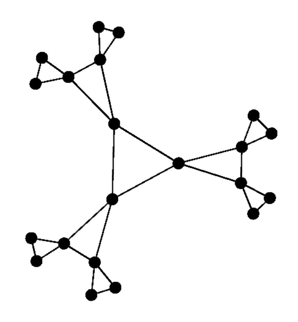
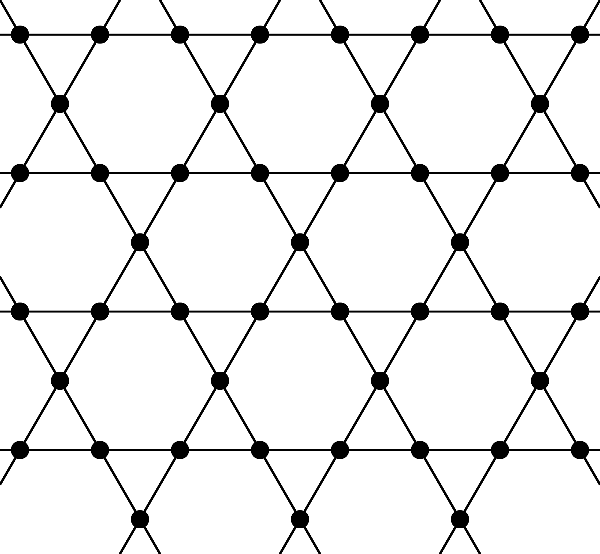
Figure 1: Pieces of the Husimi tree (left) and the Kagome lattice (right)

I.2 Results

In this article we clarify the process under which quantum selection takes place, and examine the links with thermal selection. A common heuristics states that quantum selection and thermal selection follow the same rules. This intuition, which leads to the claim that on the Kagome HAF low-energy states are coplanar, is sometimes misleading. Another claim states that quantum selection is determined by the classical frequencies in the linear spin-wave approximation. In fact there are additional terms, which do not play a role on antiferromagnetic systems but which appear in more general spin systems. We describe in detail those additional terms.

We report mathematical results, which define a function $\mu$ under which quantum selection takes place: as the spin grows, low-energy quantum states localize on the set of phase space on which both the classical energy and this function $\mu$ are minimal. We then analyse various model situations of irregular minimal classical sets in order to understand the link with thermal selection.

This article is organised as follows: Section II presents the general mathematical framework for the treatment of quantum selection in the context of spin systems. In Section III we use three toy models to illustrate the concepts and difficulties associated with quantum order by disorder. In Section IV we analyse practical examples such as the semiclassical HAF on the Kagome lattice. Section V presents a discussion of the consequences and applications of our work. The Appendix consists of exact computations which relate spin systems and Toeplitz quantization.

II Spin wave frequencies and Toeplitz quantization

In this section we expose the main mathematical ideas behind Toeplitz quantization, which allows to study spin operators in the large $S$ limit from a rigorous point of view. We report our recent results on the topic and clarify the exact procedure under which quantum selection takes place.

II.1 Harmonic oscillators in Bargmann-Fock representation

The point of view of Bargmann on the quantum harmonic oscillatorBargmann (1961); Husimi (1940), is that quantum states should be seen as holomorphic functions on the complex space $\mathbb{C}^{d}$ instead of the common choice $L^{2}(\mathbb{R}^{d})$. This idea can in fact be generalized to other phases spaces than $\mathbb{C}^{d}$, and allows to understand the large spin limit as a semiclassical limit from a rigorous point of view.

For positive $k$ (which is seen as the inverse Planck constant), holomorphic functions on $\mathbb{C}^{d}$ form a Hilbert space $B_{k}$ with the following scalar product

$$\langle u|v\rangle_{B_{k}}=\int\overline{u}(z)v(z)\exp(-k{|z|^{2}})dz.$$

We naturally exclude from the space $B_{k}$ the functions with infinite norm. Example of functions in $B_{k}$ are the monomials $z\mapsto z_{1}^{\nu_{1}}\ldots z_{d}^{\nu_{d}}$ which, once normalized, form a Hilbert base of $B_{k}$. Under this definition, $B_{k}$ naturally sits inside the space $L_{k}$ of all (not necessarily holomorphic) functions which are square-integrable with respect to the exponential weight above. The orthogonal projector $\Pi_{k}$ from $L_{k}$ to $B_{k}$ is used to define the quantum harmonic oscillator, which is the following operator on $B_{k}$:

$$T_{k}(|z|^{2})|u\rangle=\Pi_{k}(z\mapsto|z|^{2}u(z)).$$

This is a Toeplitz operator: the composition of a multiplication operator and a projection. The matrix elements are simply

$$\langle u|T_{k}(|z|^{2})|v\rangle_{B_{k}}=\int_{\mathbb{C}^{d}}\overline{u}(z)v(z)|z|^{2}\exp(-k|z|^{2})dz.$$

The monomials $z^{\nu}$ are eigenfunctions of this operator, with eigenvalues $k^{-1}(\nu_{1}+\ldots+\nu_{d}+d)$. This contrasts with the $L^{2}(\mathbb{R}^{d})$ point of view on the harmonic oscillator, where the eigenvalues are the half-integers $\hbar(\nu_{1}+\ldots+\nu_{d}+\frac{d}{2})$. This does not mean that this Toeplitz operator is not natural, or that other terms should be added; in experiments one can only measure gaps between eigenvalues, which coincide for the two settings.

The definition of the Toeplitz operator can be generalized. If $H$ is any function on $\mathbb{C}^{d}$ (which represents the classical energy on the phase space $\mathbb{C}^{d}=\mathbb{R}^{2d}$), the associated Toeplitz operator on $B_{k}$ is defined as

$$T_{k}(H)|u\rangle=\Pi_{k}(z\mapsto H(z)u(z)).$$

This defines a quantization: $T_{k}(H_{1}+H_{2})=T_{k}(H_{1})+T_{k}(H_{2})$, and in the large $k$ limit, the commutator $[T_{k}(H_{1}),T_{k}(H_{2})]$ becomes close to $-ik^{-1}T_{k}(\{H_{1},H_{2}\})$. The function $H$ associated with the operator $T_{k}(H)$, which is unique, is called the symbol of $T_{k}(H)$. In the context of spin systems it coincides with the notion of upper symbol.

Toeplitz quantization follows the Wick order: if $H:z\mapsto\overline{z}^{\alpha}z^{\beta}$, then

$$T_{k}(H)=k^{-\sum\alpha_{i}}\partial^{\alpha}z^{\beta}.$$

The Wick rule allows explicit computations for the Toeplitz quantization of any polynomial function in the coordinates.

Of great interest are Toeplitz operators associated with semipositive definite forms $Q\geq 0$. As in the harmonic case, the infimum of the spectrum is linked with the classical frequencies, but is shifted with respect to the usual quantization procedure: if $\lambda_{1},\ldots,\lambda_{r}$ are the non-zero classical frequencies for $Q$, then

$$\mu(Q):=\inf Spec(T_{k}(Q))=k^{-1}\left(\frac{1}{2}\sum_{i=1}^{r}\lambda_{i}+\frac{1}{4}tr(Q)\right).$$ (1)

The factor $tr(Q)$ is specific to Bargmann quantization. In the Weyl representation, one has instead

$$\inf Spec(Op_{W}^{\hbar}(Q))=\frac{\hbar}{2}\sum_{i=1}^{r}\lambda_{i}.$$

II.2 Toeplitz operators on spheres

Toeplitz quantization can be generalized from $\mathbb{C}^{d}$ to other phase spaces, using tools of complex geometryCharles (2003). In particular, this allows to define a quantization procedure on product of spheres: to any classical energy on a product of spheres, and any $k$, one can associate a quantum operator, acting on the tensor product of spaces $\mathbb{C}^{k+1}$. Previously $k$ was any positive real number, but now it needs to be an integer: the topology of the phase space only allows quantized values of the inverse Planck constant.

Toeplitz operators on product of spheres include spin systems (with spin $S=\frac{k}{2}$). However the quantization procedure requires some care in the computations as can be seen on Table 1.

classical	quantum ($S=\frac{k}{2}$)
$z$	$\frac{k}{k+2}S_{z}$
$x$	$\frac{k}{k+2}S_{x}$
$z^{2}$	$\frac{k^{2}}{(k,3)}S_{z}^{2}+\frac{1}{k+3}$
$zx$	$\frac{k^{2}}{2(k,3)}(S_{x}S_{z}+S_{z}S_{x})$
$z^{2}x$	$\frac{k^{3}}{(k,4)}S_{z}S_{x}S_{z}+\frac{1}{(k+3)}S_{x}$
$z^{3}$	$\frac{k^{3}}{(k,4)}S_{z}^{3}+\frac{k(3k+8)}{(k,4)}S_{z}$

Table 1: Quantization of some symbols on the sphere.
The operator $S_{z}$ has entries $-1,-1+S^{-1},\ldots,1-S^{-1},1$.
We denote $(k,j)=(k+2)(k+3)\ldots(k+j)$.

The corrective terms of order $k^{-1}$ are crucial for quantum order from disorder. The details for the computations in Table 1 are presented in the Appendix.

II.3 Quantum selection for Toeplitz operators

In a recent paperDeleporte (2016), we developed mathematical tools in order to study quantum selection for general Toeplitz operators in the large $k$ limit. We report that, in a general case (even if the set of minimal classical energy is irregular), quantum selection takes place for Toeplitz operators following a general criterion.

In order to apply our results to usual spin operators, as seen above, we need to consider Toeplitz operators with classical energy depending on $k$ in the following way:

$$f=f_{0}+k^{-1}f_{1}+k^{-2}f_{2}+\ldots,$$

where each term $f_{j}$ is a real function on the phase space. Indeed, the quantization of symbols which do not depend on $k$ only yield a deformation of the usual spin operators. The Toeplitz operator $T_{k}(f)$ is well-defined by linearity.

Quantum states with energy less than $\min(f_{0})+Ck^{-1}$ are known to localize on $Z=\{f_{0}\text{ is minimal}\}$ as $k$ grows. In a neighbourhood of any point $P_{0}$ of $Z$, the function $f_{0}$ can be approximated by its quadratic Taylor estimate $\min(f_{0})+Q$, where $Q$ is a semidefinite positive quadratic form which depends on $P_{0}$.

The selection criterion is then

$$\tilde{\mu}=\mu(Q)+f_{1},$$

in following sense: if $(u_{k})$ denotes a sequence of ground states of $T_{k}(f)$, if a set $V$ lies at positive distance from

$$\{x\in Z,\tilde{\mu}(x)=\min(\tilde{\mu})\},$$

then for every $j$ one has, as $k\to+\infty$,

$$\int_{V}|u_{k}(z)|^{2}\precsim k^{-j}.$$

The meaning of $|u_{k}(z)|^{2}$ depends on the underlying manifold (for instance, on $\mathbb{C}^{d}$ a factor $\exp(-k|z|^{2})$ must be added), but as our quantum states are defined on the whole phase space, localisation properties can be formulated in a more elementary way than in the space representation.

The quantum ground state localizes, in the large $k$ limit, only on the part of $Z$ where $\tilde{\mu}$ is minimal; at any positive distance from this set, the ground state decays faster than any negative power of $k$. In fact, if $E_{0}$ is the energy of the ground state, then any quantum eigenstate with energy less than $E_{0}+\epsilon k^{-1}$ for any $\epsilon$ localizes where $\tilde{\mu}$ is minimal.

In order to apply this result from a standard “operator-presented” quantum spin Hamiltonian in the large spin limit, one needs first to compute, not only the associated classical energy at the main order, but also the so-called “subprincipal symbol” which contains the next-order terms in the quantization procedure. For instance, starting with the operator $S_{z}^{2}$, the principal symbol is of course $z^{2}$, and from Table 1 one can compute that a more accurate representation is

$$z^{2}+k^{-1}(5z^{2}+1).$$

This subprincipal part, added to the trace and to the sum of symplectic eigenvalues of the quadratic part of the energy, yields the function $\widetilde{\mu}$ which is the selection rule. In section III we apply this method to several models.

The physical interpretation of $\widetilde{\mu}$ is the following: suppose that one wants to minimise the energy of a quantum state while constraining it to be localised at a precise point, where the classical energy has a local minimum. Then the energy of this minimal constrained state is naturally close to the classical energy, but is lifted up by quantum fluctuations. Indeed, quantum states have to spread out somewhat, and to reach parts of the phase space where the classical energy is not minimal. This energy lift is of the same order as the semiclassical parameter (here, $k^{-1}$). Then $\widetilde{\mu}$, at this point, is the $k^{-1}$ contribution to this energy lift.

In the context of spin systems, the selection rule is determined by the classical frequencies of the spin waves, and by non-trivial additional terms which must be taken care of. For the particular case of HAF systems, if each spin has the same number of neighbors, then the additional terms are constant, but on other systems on which quantum selection is studied, they can play an important role.

III Toy models

In order to understand quantum selection in the general case and in the particular case of spin systems, we first look at three simple toy models.

In the first toy model, which is the first historical example of quantum selection, thermal and quantum selection play the same role. In the second toy model, which has an irregular minimal set as does the HAF on the Kagome lattice, thermal selection is sharper than quantum selection: some classical configurations are equivalent from a quantum point of view (they share the same value of $\widetilde{\mu}$), but are discriminated by the Gibbs measure. Conversely, on the third toy model, there is no thermal selection, but quantum selection takes place.

III.1 Miniwells

The general study of quantum selection for the ground state of a Schrödinger operator was performed by Helffer and Sjöstrand Helffer and Sjöstrand (1986) who exposed a WKB construction for a quasimode associated to the lowest energy. Quantum selection occurs when the potential $V$ is minimal on a degenerate set $Z$. If $Z$ is a smooth manifold on which $V$ vanishes at order 2, the criterion for quantum selection is the trace of the square root of the Hessian matrix of $V$ at the minimal points; in this Weyl setting, it corresponds exactly to the sum of the classical frequencies for the linearized system. Even in this case it does not correspond to the criterion for thermal selection (which is the product of these frequencies).

The simplest example is the operator $P_{\hbar}=-\hbar^{2}\Delta+V$ acting on $L^{2}(\mathbb{R}^{2})$, with $V(x,y)=y^{2}(1+x^{2})$, vanishing at order two on the horizontal axis. It is already interesting to note that, though $V$ itself is not a confining potential, $P_{h}$ only has discrete spectrum because of the quantum selection.

Around every point $(x_{0},0)$ of the horizontal axis, the quadratic terms in the potential are $y^{2}(1+x_{0}^{2})$. For this quadratic potential there is one non-zero classical frequency, $\sqrt{1+x_{0}^{2}}$. This frequency is minimal at $x_{0}=0$, which is called the “miniwell” for this potential. Hence, the ground state of this operator concentrates on the point $(0,0)$, in the previous sense (for the Husimi transform).

In this setting, the value $\widetilde{\mu}$ coincides with the effective potential given by the intuition of the adiabatic approximation Douçot and Simon (1998). At $(x_{0},0)$ one can approximate the behaviour of a low-energy state in the second variable as the ground state of the quadratic transverse operator $-\hbar^{2}\partial_{y}^{2}+(1+x_{0}^{2})y^{2}$; if $e_{x_{0}}(y)$ is the ground state of this operator, then the energy of a state of the form $e_{x}(y)f(x)$ is

$$\hbar\langle f,(-\hbar\partial_{x}^{2}+\widetilde{\mu})f\rangle,$$

so that $\widetilde{\mu}$ acts as an effective potential (with new semiclassical parameter $\sqrt{\hbar}$).

III.2 Crossing points

With the Kagome lattice in mind, let us consider toy models where the minimal set of the classical energy is not a smooth manifold.

The first of this model is again a Schrödinger operator on $\mathbb{R}^{2}$, with potential $V(x,y)=x^{2}y^{2}$. The minimal set consists in the two axes, which meet at zero. On the horizontal branch $(x_{0},0)$, there is only one non-zero linear classical frequency, which is $|x_{0}|$. This frequency is minimal at zero (note that this frequency is not smooth at zero). The same applies for the vertical axis. Once again, the operator $P_{\hbar}=-\hbar^{2}\Delta+V$ only has discrete spectrum and the first eigenfunction localizes at the origin, which is also the point of thermal selection (since the local dimension of the zero modes is maximal at this point). Because of the non-regularity of the classical frequency at the crossing point, for a potential $W$ close to $V$ which is also minimal on the two axes, the quantum system will still select the crossing point.

In this setting, the Born-Oppenheimer approximation fails at the crossing point, so that there is no simpler effective model. However $\widetilde{\mu}$ still acts as an energy barrier, independently on the geometry.

A more general crossing is the Schrödinger operator on $\mathbb{R}^{3}$, with potential $V(x,y,z)=x^{2}y^{2}z^{2}$. The minimal set is the union of the three planes $\{x=0\},\{y=0\},\{z=0\}$, and the local zero dimension is maximal at the origin. However, on the plane $\{x=0\}$ the classical frequency is $|yz|$. All classical frequencies vanish identically on the three axes.

For this particular potential, there is a hierarchy of perturbations, and investigating the sub-sub-principal (order $k^{-2}$) terms will lead to concentration at the origin and discrete spectrum. However, if non-degenerate transverse modes are added, they correspond (in the adiabatic regime) to a perturbation of order $k^{-1}$, in front of which the $k^{-2}$ confinement at the origin is negligible; in the general setting, even for small perturbations, the quantum selected point can be any point on the three axes. This illustrates the discrepancy between quantum and thermal selection and shows that for the Kagome lattice, the points of quantum selection might not necessarily be the planar configurations, though those configurations have the maximal number of zero modes.

III.3 Cancelling terms

We propose an example which serves to illustrate the effects of the different terms in the process by which quantum selection takes place.

Let us consider the following one-spin Hamiltonian:

$$H=S_{z}^{2}+\Delta S_{z}S_{x}S_{z}.$$

The principal symbol of this operator is

$$h_{0}=z^{2}(1+\Delta x).$$

If $0<\Delta<1$, then $h_{0}$ is minimal on $\{z=0\}$. It looks like $h_{0}$ is smaller near $(-1,0,0)$ than near any other point, so that, at first sight, quantum order from disorder seems to take place in this setting.

Let us look at the three terms appearing in quantum selection:

1. For any minimal point, the associated linear classical frequency is zero, since the linear classical approximation is that of a free massive particle in one-dimensional space.

2. The trace of the quadratic form near a minimal point is non-zero; this term has contribution

   $$\mu=1+\Delta x$$

3. The next-order term in the expansion is

   $$h_{1}=5z^{2}-1+\Delta(9z^{2}x-x)$$

   In particular, on the set where $h_{0}$ is minimal, one has

   $$h_{1}=-1-\Delta x.$$

The set selected by quantum order by disorder is the set where $h_{1}+\mu$ is minimal, but the two terms cancel out. Hence there is no quantum selection at this order of expansion.

It can readily be seen that, if the spin $S$ is even, then $S_{z}|0\rangle=0$, so that $H|0\rangle=0$ and $|0\rangle$ is the ground state of $H$. As expected, the magnetization of $|0\rangle$ along the $x$ axis is exactly zero. Hence, there is no quantum selection in the large spin limit for this model.

More involved theoretical examples where the classical degeneracy is not lifted at any order of $S^{-1}$ include spin texturesDouçot, Kovrizhin, and Moessner (2016). In other situations, there could be no quantum selection at first order, but next-order terms could break the degeneracy. In practice, one expects additional terms (such as second nearest neighbours interactions) which will destroy exact degeneracies.

IV Examples

IV.1 Kagome lattice

The quantum HAF on the Kagome lattice is the Toeplitz quantization of the classical energy

$$\sum_{i\sim j}\mathbf{e}_{i}\cdot\mathbf{e}_{j}.$$

Here $i\sim j$ means that the two sites $i$ and $j$ are linked by an edge. The Toeplitz quantization of the symbol above is

$$\cfrac{S^{2}}{(S+1)^{2}}\sum_{i\sim j}S_{i}\cdot S_{j},$$

so that, up to a multiplicative factor, the quantization of the classical HAF is the quantum HAF. As we wish to study quantum selection, it is important that in this case $h_{1}=0$.

The low-temperature properties of the $S=\frac{1}{2}$ HAF are still unknown. Various numerical Ansätze or exact diagonalizationsIqbal, Poilblanc, and Becca (2015, 2014); Iqbal et al. (2013); Zeng and Elser (1995); Waldtmann et al. (1998); Lecheminant et al. (1997); Depenbrock, McCulloch, and Schollwöck (2012) predict a spin liquid phase with polynomial decay of correlations, which is consistent with experimentsWills and Harrison (1996). The large $S$ analysis sheds some light on this behaviour as we will see.

If $\mathbf{e}_{i}=(x_{i},y_{i},z_{i})$, since sites in the Kagome lattice are connected in triangles, up to a constant the classical energy reads

$$\sum_{\text{triangles}}\|\mathbf{e}_{i}+\mathbf{e}_{j}+\mathbf{e}_{k}\|^{2}.$$

The minimal classical set consists in configurations where, on each triangle of sites, spins form a great equilateral triangle on the sphere. This set has a highly non-trivial structure: the presence of loops of triangles makes it non-smooth. The classical minimal set for one hexagon of triangles already has a crossing point as one of the toy models, on which two smooth manifolds cross.

An interesting subset of classical minimal configurations consists in planar configurations, which form a discrete set. It is believed that quantum order by disorder selects these configurations, thus reducing the semiclassical study to a $3$ colours Potts model on the Kagome lattice (with Hamiltonian unknown so far). Some of those planar configurations have been proven Chubukov (1992) to be local minima for the function $\mu$ which is the criterion for quantum selection, but it is unknown whether these are the global minima for $\mu$ or not. The results in the $S=\frac{1}{2}$ case are compatible with this approach as there is an extensive number of coplanar states, the majority of which having no long-range order; this contrasts with the $SU(N)$-case Sachdev (1992) which would predict a unique, ordered, selected configuration.

IV.2 Simple models for the Kagome lattice

An easy case which allows to understand the large $S$ behavior of the HAF on the Kagome lattice consists in a loop of four triangles. In this situation the classical minimal set is (once accounted for the global $SO(3)$ action) the union of three circles $C_{1},C_{2},C_{3}$, two of each crossing at exactly one point. The crossing points correspond to planar configurations. There is a symmetry exchanging $C_{2}$ and $C_{3}$. In Figure 2 we plot the value of $\mu$ along $C_{1}$ and along $C_{2}$, with parameter an angle which is $0$ or $\pi$ on the crossings; this confirms the general belief that $\mu$ is minimal on planar configurations.

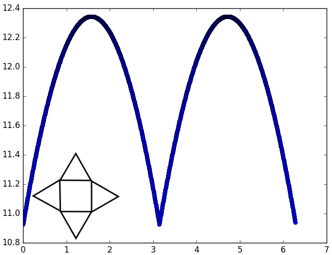
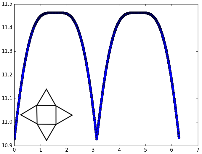
Figure 2: Numerical plot of $\mu$ for a loop of 4 triangles (insets), along $C_{1}$ (left) and $C_{2}$ (right).

The Husimi tree, proposed by Douçot and SimonDouçot and Simon (1998), also serves as a toy model for the study of the Kagome lattice. It is depicted on Figure 1.

The advantage of this model is that the classical minimal set is much simpler than on the Kagome lattice. Indeed, on the Husimi tree, once the three vectors on a parent triangle are chosen along a great equilateral triangle on the sphere, there is one degree of freedom in the choice of the spins for each child triangle. Thus the minimal set is a torus of dimension $\sharp(\text{triangles})-1$, parametrised by the angles between the equilateral triangles at neighbouring sites.

Douçot and Simon Douçot and Simon (1998) reported that the classical frequencies are not constant on the classical minimal set: in particular, in this situation there is quantum selection (the selected points are presumed to be coplanar configurations except for the spins at the leaves which are free), but there is no thermal selection since there are equivalent for a class of phase space transformations which preserve the volume.

IV.3 Anisotropic XXZ chain

Let us take up from an example proposed by Douçot and Simon Douçot and Simon (1998) and define the following Hamiltonian acting on a closed chain of $N$ spins:

$$H=J\sum_{i}S_{i}\cdot S_{i+1}+\sum_{i}S^{z}_{i}(S_{i+1}^{z}-S_{i}^{z}).$$

The principal term in the classical energy is

$$h_{0}=J\sum_{i}\mathbf{e}_{i}\cdot\mathbf{e}_{i+1}+\sum_{i}z_{i}(z_{i}-z_{i+1}).$$

The next-order contribution is

$$h_{1}=2J\sum_{i}\mathbf{e}_{i}\cdot\mathbf{e}_{i+1}+\sum_{i}(-2z_{i}z_{i+1}+5z_{i}^{2}-1).$$

If $J<0$, the minimum of $h_{0}$ is reached on ferromagnetic configurations $\{\mathbf{e}_{i}=\mathbf{e}\}$, indexed by $\mathbb{S}^{2}$.

Near any of these minimal configurations, the linear spin wave theory is the same, up to a factor $-J+1-z^{2}$ in the potential. Hence $\mu$ is minimal as $z=0$.

On ferromagnetic ordered configurations, one has

$$h_{1}=JN+3Nz^{2}.$$

Again $h_{1}$ is smaller when $z=0$. The sum $\mu+h_{1}$, which is the criterion for quantum selection, is minimal as $z=0$, hence the ground state is located on this set.

V Conclusion

V.1 Quantum versus thermal selection

In this paper, we reported evidence that quantum order by disorder does not have the same rules as thermal order by disorder. In experimental settings of low-temperature quantum systems, there is competition between quantum and thermal selection. We present an analysis of orders of magnitude.

On the system $SrCrGaO$ which is an experimental realization of the Kagome lattice, the interaction strength $J$ is presumedHarris, Kallin, and Berlinsky (1992) to be of order

$$\frac{J}{k_{B}}\simeq 50K.$$

In experimental realizations, the spin $S$ cannot be very large so that the order of magnitude of the contribution $\mu+h_{1}$ is also of order $10K\times k_{B}$. This means that, below these temperatures, quantum selection predominates over thermal selection, since the magnitude of the quantum fluctuations is much greater. On the Kagome lattice there is no competition presumed between quantum and thermal selection, but in other cases it could even lead to a phase transition from thermal order (at medium temperatures) to quantum order (at very low temperatures). The temperatures involved in this analysis can be reached for large systems by modern experimental methods.

In our recent paper Deleporte (2016) we also computed the relative contributions at low temperature on systems for which the quantum selection criterion $\mu+h_{1}$ is minimal at two points, one of which is a regular “miniwell” point, the other a crossing point. In this situation, if the temperature is such that thermal effects are of the same order as quantum effects, then the crossing point will be selected (the quantum fluctuations do not see the difference between the two points, and the thermal fluctuations select the one with maximal local zero dimension). However at lower temperatures, the regular point will be selected. The interpretation is that $\mu+h_{1}$ acts as an effective Hamiltonian, which is smooth on the miniwell, but which is typically non-regular at the crossing point (see Figure 2). This confinement leads to an increased quantum energy (this shift is of order $S^{-4/3}$). Hence there are more low-energy quantum states near the miniwell than near the crossing point. This is a theoretical instance of a phase transition, which is of course very peculiar (since $\mu+h_{1}$ reaches the same value at two very different points).

V.2 Selection on the Kagome lattice

The actual computation of $\mu$ on examples, even as simple as a chain of triangles, requires the full diagonalization of a matrix whose size grows with the number of spins, at each minimal point. Variational approaches allow to show that special (usually planar) configurations are critical points for $\mu$ (the first derivative of $\mu$ vanishes at these points), but to show that these configurations are global minima requires additional techniques.

As illustrated in Section III, the local geometry of the minimal classical set plays a very important role. Points near which the classical minimal set is a smooth manifold are now quite well understood from a mathematical point of view. On a point where exactly two manifolds cross, there is a chance that quantum order by disorder selects the crossing, especially in symmetrical situations for which the function $\mu$ reaches a local minimum at the crossing. Conversely, if three or more manifolds cross at a point, with model the boundary of a hypercube, then the crossing point has no reason to be selected by the quantum system.

We believe that, near planar configurations on the Kagome lattice, the local structure of the classical minimal set is a direct product of structures with two manifolds crossing , with quartic non-degenerate part (that is, they follow the model case above). Indeed, the quadratic and quartic terms in the energy, near a planar configuration, do not depend on the particular planar configuration, so that as soon as for one configuration one has a product of structures as above, it is the case for all configurations.

On systems where the classical minimal set is non smooth, such as the Kagome lattice, the parametrisation of this set is already a challenge. Numerical techniques which do not involve knowledge of the minimal set should be of help in tackling this problem.

V.3 Tunnelling

To conclude with, we address the issue of exponential precision in estimates related to Toeplitz operators. This problem is relevant in the context of tunnelling: it is generally hoped that, in the presence of symmetries, the ground state will tunnel between various configurations, and the spectral gap (or the inverse time needed for a quantum state to go from one configuration to another) will be of order $\exp(-cS)$ in the large spin limit, where $c$ is a “tunnelling rate”, related to some classical action.

Various attemptsGarg and Kim (1992); Awschalom et al. (1992); Garg and Kim (1990); Chudnovsky and Gunther (1988); Auerbach and Larson (1991); Anderson (1956); von Delft and Henley (1993) have been made to study this phenomenon in the setting of spin systems, mainly by removing two antipodal points on the phase space (the sphere), thus formally transforming the phase space into $\mathbb{R}\times\mathbb{S}^{1}$ in which usual (Weyl) quantization takes place with quantum state space $L^{2}(\mathbb{S}^{1})$. However, it is doubtful that these attempts yield the correct tunnelling rate. First, this manipulation changes the quantization procedure, and it is unclear whether there is a way to perform the computations which is consistent with the initial problem up to an error of order $S^{-1}$, let alone an exponentially small error. Second, rates of decay of order $\exp(-c\hbar^{-1})$ are notoriously delicate even in the simplest geometrical setting of Weyl quantization on $\mathbb{R}^{2n}$, as detailed by MartinezMartinez (2002). The basic difficulty is that one needs to extend data in complex space, which can be done only if the classical energy is real analytic, and only to a small distance from the real space. This puts a limit on the actual tunnelling rate. Lower bounds (Agmon estimates) on the tunnelling rate for Toeplitz operators were recently obtained by the authorDeleporte (2018).

*

Appendix A Computation of Toeplitz operators on the sphere

For the particular case of the sphere, one can build Toeplitz operators as on $\mathbb{C}^{d}$ via the stereographic projection, which maps the sphere minus the north pole onto $\mathbb{C}$ in a holomorphic way.

Via this transformation, quantum states are holomorphic functions on $\mathbb{C}$ which have finite norm under the following Hermitian structure:

$$\langle f|g\rangle_{H_{k}}=\frac{k+1}{\pi}\int_{\mathbb{C}}\frac{\overline{f}(w)g(w)}{(1+|w|^{2})^{k+2}}dw.$$

The space $H_{k}$ consists of polynomials of degree less than $k$. As for the flat case, the monomials are orthogonal but not normalized. A Hilbert basis of $H_{k}$ is given by

$$e_{j,k}:z\mapsto\sqrt{\cfrac{k+1}{\pi}\binom{k}{j}}z^{j}.$$

To prove this (and perform further computations), we use the fact that, for $0\leq j\leq k$:

$$\int_{0}^{+\infty}\cfrac{u^{j}}{(1+u)^{k+2}}=\cfrac{1}{k+1}\binom{k}{j}^{-1}.$$

Let us compute the Toeplitz quantization of simple functions defined on the sphere.

The height $z$ is mapped, via the stereographic projection, in the map

$$w\mapsto\cfrac{|w|^{2}-1}{|w|^{2}+1}.$$

Since this function is radial, the matrix elements $\langle e_{j,k}|T_{k}(z)|e_{j^{\prime},k}\rangle_{H_{k}}$ are zero for $j\neq j^{\prime}$. Moreover,

$$\langle e_{j,k}|T_{k}(z)|e_{j,k}\rangle_{H_{k}}=\cfrac{2j-k}{k+2}.$$

Hence, in this basis, the operator $T_{k}(z)$ is $\cfrac{k}{k+2}$ times a diagonal operator with equidistributed diagonal values from $-1$ to $1$; that is, the spin operator $S_{z}$ with $2S=k$. The states $e_{j,k}$ corresponds to spin states $|S,m\rangle$ with $m=j-S$.

The abscissa $x$ is mapped, via the stereographic projection, into the map

$$w\mapsto\cfrac{2Re(w)}{1+|w|^{2}}.$$

This is the sum of a function of winding number $-1$ and a function of winding number $1$. Hence the matrix of $T_{k}(x)$ in the natural basis is zero except on the over- and underdiagonal. The matrix elements are

$$\langle e_{j,k}|T_{k}(x)|e_{j+1,k}\rangle_{H_{k}}=\cfrac{\sqrt{(k-j)(j+1)}}{k+2}.$$

In this basis the matrix of the operator $T_{k}(x)$ is $\frac{k}{k+2}S_{x}$.

By this method, the Toeplitz quantization of any polynomial in the coordinates can be computed; this yields Table 1.

References

- Anderson (1956) Anderson, P. W., Physical Review 102, 1008 (1956).
- Anderson (1973) Anderson, P. W., Materials Research Bulletin 8, 153 (1973).
- Auerbach and Larson (1991) Auerbach, A. and Larson, B. E., Physical review letters 66, 2262 (1991).
- Awschalom et al. (1992) Awschalom, D. D., Smyth, J. F., Grinstein, G., DiVincenzo, D. P., and Loss, D., Physical review letters 68, 3092 (1992).
- Bargmann (1961) Bargmann, V., Communications on pure and applied mathematics 14, 187 (1961).
- Charles (2003) Charles, L., Communications in Mathematical Physics 239, 1 (2003).
- Chubukov (1992) Chubukov, A., Physical Review Letters 69, 832 (1992).
- Chudnovsky and Gunther (1988) Chudnovsky, E. M. and Gunther, L., Physical review letters 60, 661 (1988).
- Deleporte (2016) Deleporte, A., arXiv:1610.05902 [math-ph] (2016).
- Deleporte (2018) Deleporte, A., In preparation (2018).
- von Delft and Henley (1993) von Delft, J. and Henley, C. L., Physical Review B 48, 965 (1993).
- Depenbrock, McCulloch, and Schollwöck (2012) Depenbrock, S., McCulloch, I. P., and Schollwöck, U., Physical review letters 109, 067201 (2012).
- Douçot, Kovrizhin, and Moessner (2016) Douçot, B., Kovrizhin, D. L., and Moessner, R., Physical Review B 93, 094426 (2016).
- Douçot and Simon (1998) Douçot, B. and Simon, P., Journal of Physics A: Mathematical and General 31, 5855 (1998).
- Garg and Kim (1990) Garg, A. and Kim, G.-H., Journal of Applied Physics 67, 5669 (1990).
- Garg and Kim (1992) Garg, A. and Kim, G.-H., Physical Review B 45, 12921 (1992).
- Harris, Kallin, and Berlinsky (1992) Harris, A. B., Kallin, C., and Berlinsky, A. J., Physical Review B 45, 2899 (1992).
- Harris et al. (1997) Harris, M. J., Bramwell, S. T., McMorrow, D. F., Zeiske, T. H., and Godfrey, K. W., Physical Review Letters 79, 2554 (1997).
- Helffer and Sjöstrand (1986) Helffer, B. and Sjöstrand, J., Current topics in partial differential equations , 133 (1986).
- Husimi (1940) Husimi, K., Proceedings of the Physico-Mathematical Society of Japan. 3rd Series 22, 264 (1940).
- Iqbal et al. (2013) Iqbal, Y., Becca, F., Sorella, S., and Poilblanc, D., Physical Review B 87, 060405 (2013).
- Iqbal, Poilblanc, and Becca (2014) Iqbal, Y., Poilblanc, D., and Becca, F., Physical Review B 89, 020407 (2014).
- Iqbal, Poilblanc, and Becca (2015) Iqbal, Y., Poilblanc, D., and Becca, F., Physical Review B 91, 020402 (2015).
- Lago et al. (2010) Lago, J., Živković, I., Malkin, B. Z., Fernandez, J. R., Ghigna, P., de Réotier, P. D., Yaouanc, A., and Rojo, T., Physical review letters 104, 247203 (2010).
- Lecheminant et al. (1997) Lecheminant, P., Bernu, B., Lhuillier, C., Pierre, L., and Sindzingre, P., Physical Review B 56, 2521 (1997).
- Martinez (2002) Martinez, A., An Introduction to Semiclassical and Microlocal Analysis. 2002, Universitext (Springer, 2002).
- Matsuhira et al. (2002) Matsuhira, K., Hinatsu, Y., Tenya, K., Amitsuka, H., and Sakakibara, T., Journal of the Physical Society of Japan 71, 1576 (2002).
- Note (1) If the minimal set is infinite, the number of eigenstates with energy less than for any tends to as .
- Note (2) An example of such a direct product is the Schrodinger opertor on with potential . At the point four manifolds cross as a cartesian square of the crossing of two manifolds at a point, not as the corner of a hypercube.
- Sachdev (1992) Sachdev, S., Physical Review B 45, 12377 (1992).
- Villain et al. (1980) Villain, J., Bidaux, R., Carton, J.-P., and Conte, R., Journal de Physique 41, 1263 (1980).
- Waldtmann et al. (1998) Waldtmann, C., Everts, H. U., Bernu, B., Lhuillier, C., Sindzingre, P., Lecheminant, P., and Pierre, L., The European Physical Journal B-Condensed Matter and Complex Systems 2, 501 (1998).
- Wills and Harrison (1996) Wills, A. S. and Harrison, A., Journal of the Chemical Society, Faraday Transactions 92, 2161 (1996).
- Zeng and Elser (1995) Zeng, C. and Elser, V., Physical Review B 51, 8318 (1995).