Linguistic Search Optimization for Deep Learning Based LVCSR

1 Motivation and General Ideas

Recent advances in deep learning based large vocabulary continuous speech recognition (LVCSR) invoke growing demands in large scale speech transcription. The inference process of a speech recognizer is to find a sequence of labels whose corresponding acoustic and language models best match the input feature [1]. The main computation includes two stages: acoustic model (AM) inference and linguistic search (weighted finite-state transducer, WFST). Large computational overheads of both stages hamper the wide application of LVCSR.

To reduce computation of the first stage, researchers have proposed a variety of efficient forms of AMs, including novel structures [2, 3], quantization  [4, 5] and frame-skipping [6]. Meanwhile, algorithmic improvement of linguistic search, e.g. pruning [7], rescoring [8] and lookahead [9, 10], was the mainstream approach to speed up the second stage in the past.

This work mainly focuses on linguistic search. Despite the WFST based LVCSR approach has been improved for several decades, two fundamental deficiencies remain: i) The WFST search space is large and its graph traversal algorithms are conducted at each frame, e.g. frame synchronous Viterbi beam decoding (FSD). ii) Most of these algorithms are originally serial algorithms and parallelizing them is non-trivial.

Benefit from stronger classifiers, deep learning, and more powerful computing devices, we propose general ideas and some initial trials to solve these fundamental problems:

• Reduce the search complexity by end-to-end modeling

Recent advances in more potent neural networks enable stronger modeling effects in the context and the history of the sequential modeling [11, 12, 13, 14, 15]. More labeled data further alleviates the sparseness and generalization problem in the modeling. Thus, it is promising to decompose the sequence into larger model granularities. Research has been conducted on different model granularities from frame level to the whole sequence [16, 17, 18, 19, 20]. e.g., in [17], a word level deep learning based acoustic model is trained on 125K hours labeled data and outperforms models with smaller granularity. We propose to change the frequency of Viterbi search from each feature frame to each label output. Correspondingly, a post-processing is applied on the frame level acoustic model outputs to obtain the label outputs: i) Decide whether there is a label output at the current frame or not. ii) If so, conduct the search process. If not, discard the current output. Thus the post-processing can be viewed as the approximated probability calculation of each output label. Based on this framework, the larger model granularities we take, the less search complexity we obtain.

• Accelerate the search speed using parallel computing

GPU-based parallel computing is another potential direction which utilizes a large number of units to parallelize the computation. As common language models (LM) can be expressed as WFSTs, the idea is to parallelize WFST graph traversal algorithms. Our initial work parallelizes Viterbi algorithm [21] and redesigns it to fully utilize parallel computing devices nowadays, e.g. Graphics Processing Units (GPU) and Field-Programmable Gate Arrays (FPGA). To utilize large LMs in the 2nd pass and support rich post-processing, our design is to decode the WFSTs and generate exact lattices [22]. The decoder remains to be general-purpose and does not impose special requirements on the form of AM or LM. The ideas to apply GPU parallel computing in WFST decoding include: i) Abstract the dynamic programming in the Viterbi algorithm as thread synchronization using atomic GPU operations. ii) Propose a load balancing strategy for parallel WFST search scheduling among GPU threads. iii) Parallelize exact lattice generation and pruning algorithms. Similar ideas can be applied to other WFST algorithms, e.g. determinization and minimization [7], and speedups of them can be expected.

2 Label Synchronous Framework

The search process is proposed to change from the feature level to the label level, i.e. label synchronous decoding (LSD) [23, 24]. Within the label inference, a post-processing is applied on the frame level acoustic model outputs. The formulation and implementation are discussed on CTC [25] and LF-MMI [26].

During inference stage, Viterbi beam search of CTC model [25] can be expressed as,

$$\vspace{-0.5em}\mathbf{w}^{*}=\mathop{\arg\!\max}\limits_{\mathbf{w}}\left\{P(\mathbf{w})\mathop{\max}\limits_{\mathbf{l}_{\mathbf{w}}}\frac{\prod_{l\in\mathbf{l}_{\mathbf{w}}}P(l|\mathbf{x})}{P(\mathbf{l}_{\mathbf{w}})}\right\}$$ (1)

where $\mathbf{x}$ is the feature sequence, $\mathbf{w}$ is a word sequence and ${\mathbf{w}}^{*}$ is the best word sequence. $\mathbf{l}_{\mathbf{w}}$ denotes the label sequence, e.g. the phoneme sequence, corresponding to $\mathbf{w}$. Within the calculation of $P(l|\mathbf{x})$, a post-processing is proposed on the frame level neural network outputs, $P(\pi|\mathbf{x})$. Here, the set of common $\tt blank$ frames are defined as: $U=\{u:y^{u}_{\tt{blank}}>\mathcal{T}\}$, where $y^{u}_{\tt{blank}}$ is the probability of the $\tt blank$ unit at frame $u$. With a softmax layer in the CTC model, if the $\tt blank$ acoustic score is large enough and approaching a constant of $1$, it can be regarded that all competing paths share the same span of the $\tt blank$ frame. Thus ignoring the scores of the frame does not affect the acoustic score rank in decoding:

$$\begin{split}P(l|\mathbf{x})\triangleq\sum_{\pi\in\mathcal{B}(\mathbf{l})}\ \prod_{\pi}P(\pi|\mathbf{x})\\ \simeq\sum_{\pi\in\mathcal{B}(\mathbf{l})}\ \prod_{\pi\in U}{y_{b_{l}}^{u}}{\prod_{\pi\not\in U}{y_{p_{l}}^{u}}}\simeq\sum_{\pi\in\mathcal{B}(\mathbf{l})}\ {\prod_{\pi\not\in U}{y_{p_{l}}^{u}}}\end{split}$$ (2)

where $\mathcal{B}$ is a one-to-many mapping between labels, e.g. phonemes, and CTC states. LSD is summarized as Algorithm 1. The main difference compared with FSD Viterbi algorithm is the introduction of $isBlankFrame(F)$ to detect whether a frame is $\tt blank$ or not. Recently, novel HMM topology was proposed in [26, 6], which holds a similar one-to-many mapping as $\mathcal{B}$ function of CTC. The three-state HMM contains a state simulating the function of $\tt blank$. Thus similar post-processing as Equation (2) and its corresponding algorithm can be derived.

Algorithm 1 Label Synchronous Viterbi Beam Search for CTC (Inputs: start and end nodes, token queue, time frames)

1:procedure  LSD for CTC (S, E, Q, T)

2:     $Q\leftarrow S$ $\triangleright$ initialization with start node

3:     for each $t\in[1,T]$ do $\triangleright$ frame-wise NN Propagation

4:         $F\leftarrow NNPropagate(t)$

5:         if !isBlankFrame($F$) then $\triangleright$ phone-wise decoding

6:              $Q\leftarrow ViterbiBeamSearch(F,Q)$               

7:     $\hat{B}\leftarrow finalTransition(E,S,Q)$ $\triangleright$ to reach end node

8:     backtrace($\hat{B}$)

The decoding complexity reduction from FSD to LSD is as Equation (3), where $T$ is the number of frames, $|L^{\prime}|$ and $|W|$ are sizes of label set and vocabulary. The number of $\tt blank$ frames, $|U|$, is always approaching T. Thus FSD is greatly sped up.

$$\vspace{-0.5em}\begin{split}\mathbb{C}\propto\ T\cdot|L^{\prime}|\cdot|W|\ \ \ \Rightarrow\ \ \ (T-|U|)\cdot|L^{\prime}|\cdot|W|\end{split}$$ (3)

Experiments on Switchboard [27] show the speedup as Figure 1.

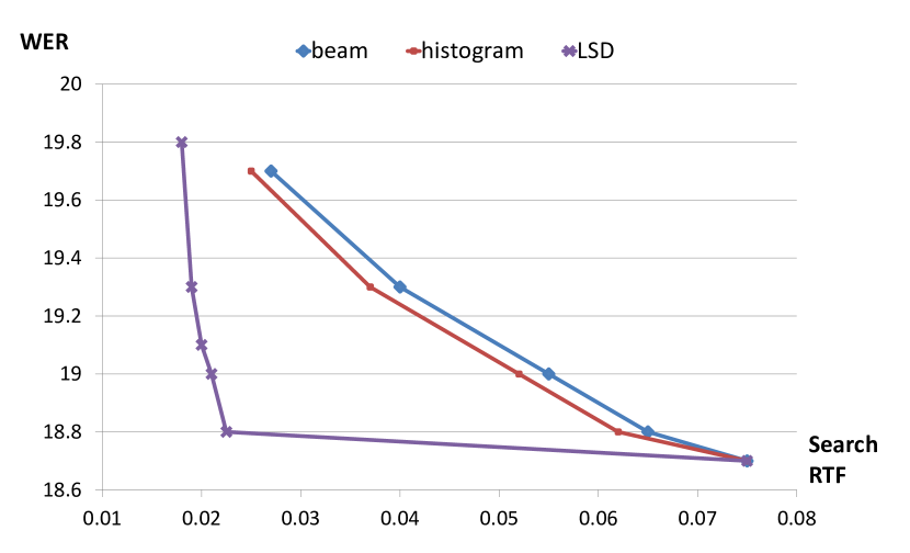
Figure 1: hub5e-swb WER versus Search Real-time Factor (RTF) in CTC Obtained by LSD and Other Pruning Methods.

3 GPU-based Parallel WFST Decoding

Figure 2 shows the framework of parallel Viterbi beam search [28]. The procedure of decoding is similar to the CPU version [29] but works in parallel with specific designs. Load balancing controls the thread parallelism over both WFST states and arcs. Two GPU concurrent streams perform decoding and lattice-pruning in parallel launched by CPU asynchronous calls.

We parallelize token passing algorithm [30] in two levels. Tokens in different states are processed parallelly. For each token, we traverse its out-going arcs in parallel as well. Because WFST states might have different numbers of out-going arcs, the allocation of states and arcs to threads can result in load imbalance. We use a dispatcher in charge of global scheduling, and make $N$ threads as a group ($N=32$) to process arcs from a token. When the token is processed, the group requests a new token from the dispatcher. We implement task dispatching as an atomic operation [31]. Figure 2 shows an example.

At each frame, the Viterbi path is obtained by a token recombination procedure, where a min operation is performed on each state over all of its incoming arcs (e.g. state 7 in Figure 2 and the incoming arcs from state 2, 5 and 7), to compute the best cost and the corresponding predecessor of that state. We abstract this process as thread synchronization using atomic GPU operations. After finishing all synchronization, we aggregate survived tokens exploiting thread parallelism. We also parallelize exact lattice generation and pruning algorithms with similar ideas, described in [28].

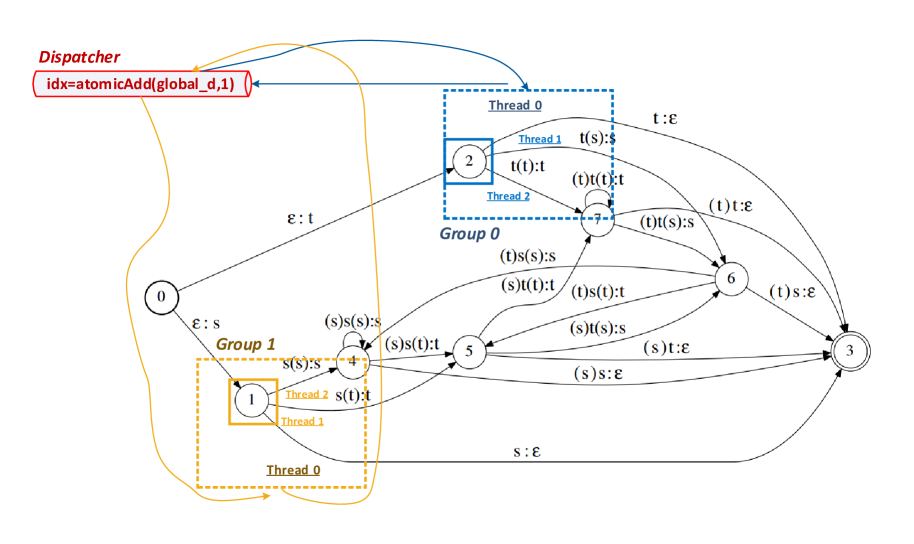
Figure 2: Example of Dynamic Load Balancing. The dashed box denotes a CUDA cooperative group and different groups are with different colors. Each group is controlled by Thread 0 of it. After processing all the forward links of a state, Thread 0 accesses the dispatcher and the next token is dynamically decided by atomic operation. Group 0 and 1 work in parallel.

Experiments on Switchboard show that the proposed GPU decoder significantly and consistently speeds up CPU counterparts in varieties of GPU architectures, LMs and AMs. The implementation of this work is open-sourced .

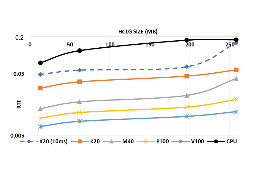
Figure 3: LM Size, Frame Rates and Architectures Comparison.

4 Future works

Our general ideas to reduce the computation of speech applications are two folds: reduce the search complexity by end-to-end modeling and accelerate WFST algorithms using parallel computing. For the first part, LSD in both discriminative and generative sequence models should be fully investigated. Integrating LSD as a sub-sampling module in the sequence-to-sequence framework is another direction [32]. Keyword spotting and confidence measures in this framework needs to be considered [33, 34, 35]. For the second part, the initial work in Viterbi decoding can be extended to most of WFST graph traversal algorithms [7]. According to specific application scenarios, parallel implementations of various devices (e.g. CPU, GPU and FPGA) can be considered. Neural network language models should be taken into account [36].

5 Acknowledgements

I express sincere gratitude to my advisors, Kai Yu and Yanmin Qian. I thank the speech technology group of AISpeech Ltd. for infrastructure support and valuable technical discussions. I thank my internship mentors, Jasha Droppo, Jinyu Li, Daniel Povey, Justin Luitjens, Christian Fuegen and Yongqiang Wang.

References

- [1] X. Huang, A. Acero, and H.-W. Hon, Spoken Language Processing: A Guide to Theory, Algorithm, and System Development, 1st ed. Upper Saddle River, NJ, USA: Prentice Hall PTR, 2001.
- [2] J. Xue, J. Li, D. Yu, M. Seltzer, and Y. Gong, “Singular value decomposition based low-footprint speaker adaptation and personalization for deep neural network,” in Acoustics, Speech and Signal Processing (ICASSP), 2014 IEEE International Conference on. IEEE, 2014, pp. 6359–6363.
- [3] V. Peddinti, Y. Wang, D. Povey, and S. Khudanpur, “Low latency acoustic modeling using temporal convolution and lstms,” IEEE Signal Processing Letters, vol. 25, no. 3, pp. 373–377, 2018.
- [4] I. McGraw, R. Prabhavalkar, R. Alvarez, M. G. Arenas, K. Rao, D. Rybach, O. Alsharif, H. Sak, A. Gruenstein, F. Beaufays et al., “Personalized speech recognition on mobile devices,” in Acoustics, Speech and Signal Processing (ICASSP), 2016 IEEE International Conference on. IEEE, 2016, pp. 5955–5959.
- [5] X. Xiang, Y. Qian, and K. Yu, “Binary deep neural networks for speech recognition,” Proc. Interspeech 2017, pp. 533–537, 2017.
- [6] G. Pundak and T. N. Sainath, “Lower frame rate neural network acoustic models.” in Interspeech, 2016, pp. 22–26.
- [7] M. Mohri, F. Pereira, and M. Riley, “Weighted finite-state transducers in speech recognition,” Computer Speech & Language, vol. 16, no. 1, pp. 69–88, 2002.
- [8] T. Hori, C. Hori, and Y. Minami, “Fast on-the-fly composition for weighted finite-state transducers in 1.8 million-word vocabulary continuous speech recognition,” in Eighth International Conference on Spoken Language Processing, 2004.
- [9] H. Soltau and G. Saon, “Dynamic network decoding revisited,” in Automatic Speech Recognition & Understanding, 2009. ASRU 2009. IEEE Workshop on. IEEE, 2009, pp. 276–281.
- [10] D. Nolden, R. Schlüter, and H. Ney, “Search space pruning based on anticipated path recombination in lvcsr,” in Interspeech, 2012.
- [11] H. Sak, A. Senior, and F. Beaufays, “Long short-term memory recurrent neural network architectures for large scale acoustic modeling,” in Fifteenth Annual Conference of the International Speech Communication Association, 2014.
- [12] Y. Qian, M. Bi, T. Tan, and K. Yu, “Very deep convolutional neural networks for noise robust speech recognition,” IEEE/ACM Transactions on Audio, Speech, and Language Processing, vol. 24, no. 12, pp. 2263–2276, 2016.
- [13] Z. Chen, J. Droppo, J. Li, and W. Xiong, “Progressive joint modeling in unsupervised single-channel overlapped speech recognition,” IEEE/ACM Transactions on Audio, Speech and Language Processing (TASLP), vol. 26, no. 1, pp. 184–196, 2018.
- [14] Z. Chen and J. Droppo, “Sequence modeling in unsupervised single-channel overlapped speech recognition.” ICASSP, 2018.
- [15] M. Huang, Y. You, Z. Chen, Y. Qian, and K. Yu, “Knowledge distillation for sequence model.” in Interspeech 2018.
- [16] D. Amodei et al., “Deep speech 2: End-to-end speech recognition in english and mandarin,” arXiv preprint arXiv:1512.02595, 2015.
- [17] H. Soltau, H. Liao, and H. Sak, “Neural speech recognizer: Acoustic-to-word lstm model for large vocabulary speech recognition,” arXiv preprint arXiv:1610.09975, 2016.
- [18] R. Collobert, C. Puhrsch, and G. Synnaeve, “Wav2letter: an end-to-end convnet-based speech recognition system,” arXiv preprint arXiv:1609.03193, 2016.
- [19] H. Sak, A. Senior, K. Rao, and F. Beaufays, “Fast and accurate recurrent neural network acoustic models for speech recognition,” arXiv preprint arXiv:1507.06947, 2015.
- [20] W. Chan, “End-to-end speech recognition models,” Ph.D. dissertation, Carnegie Mellon University Pittsburgh, PA, 2016.
- [21] G. D. Forney, “The viterbi algorithm,” Proceedings of the IEEE, vol. 61, no. 3, pp. 268–278, 1973.
- [22] D. Povey, M. Hannemann, G. Boulianne, L. Burget, A. Ghoshal, M. Janda, M. Karafiát, S. Kombrink, P. Motlíček, Y. Qian et al., “Generating exact lattices in the wfst framework,” in Acoustics, Speech and Signal Processing (ICASSP), 2012 IEEE International Conference on. IEEE, 2012, pp. 4213–4216.
- [23] Z. Chen, W. Deng, T. Xu, and K. Yu, “Phone synchronous decoding with ctc lattice,” in Interspeech 2016, 2016, pp. 1923–1927.
- [24] Z. Chen, Y. Zhuang, Y. Qian, and K. Yu, “Phone synchronous speech recognition with ctc lattices,” IEEE/ACM Transactions on Audio, Speech, and Language Processing, vol. 25, no. 1, pp. 86–97, Jan 2017.
- [25] A. Graves, S. Fernández, F. Gomez, and J. Schmidhuber, “Connectionist temporal classification: labelling unsegmented sequence data with recurrent neural networks,” in Proceedings of the 23rd international conference on Machine learning. ACM, 2006, pp. 369–376.
- [26] D. Povey, V. Peddinti, D. Galvez, P. Ghahrmani, V. Manohar, X. Na, Y. Wang, and S. Khudanpur, “Purely sequence-trained neural networks for asr based on lattice-free mmi,” Submitted to Interspeech, 2016.
- [27] J. J. Godfrey, E. C. Holliman, and J. McDaniel, “Switchboard: Telephone speech corpus for research and development,” in Acoustics, Speech, and Signal Processing, 1992. ICASSP-92., 1992 IEEE International Conference on, vol. 1. IEEE, 1992, pp. 517–520.
- [28] Z. Chen, J. Luitjens, H. Xu, Y. Wang, D. Povey, and S. Khudanpur, “A gpu-based wfst decoder with exact lattice generation,” arXiv preprint arXiv:1804.03243, 2018.
- [29] D. Povey, A. Ghoshal, G. Boulianne, L. Burget, O. Glembek, N. Goel, M. Hannemann, P. Motlicek, Y. Qian, P. Schwarz et al., “The kaldi speech recognition toolkit,” in IEEE 2011 workshop on automatic speech recognition and understanding, no. EPFL-CONF-192584. IEEE Signal Processing Society, 2011.
- [30] S. Young, “The htk book version 3.4. 1,” 2009.
- [31] “Cuda toolkit documentation,” http://docs.nvidia.com/cuda/, accessed: 2018-03-17.
- [32] Z. Chen, Q. Liu, H. Li, and K. Yu, “On modular training of neural acoustics-to-word model for lvcsr,” in ICASSP, April 2018.
- [33] Z. Chen, Y. Qian, and K. Yu, “A unified confidence measure framework using auxiliary normalization graph,” in International Conference on Intelligent Science and Big Data Engineering. Springer, 2017, pp. 123–133.
- [34] Z. Chen, Y. Zhuang, and K. Yu, “Confidence measures for ctc-based phone synchronous decoding,” in Acoustics, Speech and Signal Processing (ICASSP), 2017 IEEE International Conference on. IEEE, 2017, pp. 4850–4854.
- [35] Z. Chen, Y. Qian, and K. Yu, “Sequence discriminative training for deep learning based acoustic keyword spotting,” Speech Communication, 2018.
- [36] H. Xu, T. Chen, D. Gao, Y. Wang, K. Li, N. Goel, Y. Carmiel, D. Povey, and S. Khudanpur, “A pruned rnnlm lattice-rescoring algorithm for automatic speech recognition,” 2017.