Multi-threshold Change Plane Model: Estimation Theory and Applications in Subgroup Identification

Abstract

We propose a multi-threshold change plane regression model which naturally partitions the observed subjects into subgroups with different covariate effects. The underlying grouping variable is a linear function of covariates and thus multiple thresholds form parallel change planes in the covariate space. We contribute a novel 2-stage approach to estimate the number of subgroups, the location of thresholds and all other regression parameters. In the first stage we adopt a group selection principle to consistently identify the number of subgroups, while in the second stage change point locations and model parameter estimates are refined by a penalized induced smoothing technique. Our procedure allows sparse solutions for relatively moderate- or high-dimensional covariates. We further establish the asymptotic properties of our proposed estimators under appropriate technical conditions. We evaluate the performance of the proposed methods by simulation studies and provide illustration using two medical data. Our proposal for subgroup identification may lead to an immediate application in personalized medicine.

Keywords: Induced smoothing; Penalty function; Precision medicine; Subgroup identification.

1 Introduction

Individualized learning and modeling has become increasingly important in statistics and computer science, especially for solving the personalized medical treatment problems. The traditional “one size fits all” approach is unable to detect important patterns in the sub-populations and make the best personalized predictions for specific individuals. For example, in the fight against cancer and other diseases, it is difficult to recommend a treatment that works for all patients. Consequently the rise of precision medicine and analysis of electronic health record data motivates researchers to identify meaningful subgroups and model the relationships between response and predictors differently across the subgroups.

Earlier development in personalized medicine focused on determining dynamic treatment regimes at multiple stages. Popular model based methods for estimating the optimal individualized treatment regimes include the Q-learning (Qian and Murphy, 2011; Goldberg and Kosorok, 2012) and the A-learning (Murphy, 2003; Robins, 2004; Schulte et al., 2014), which models interactions between the treatments and covariates and is more robust to model misspecification than Q-learning. Zhao et al. (2012) introduced the framework of outcome weighted learning (O-learning) to directly find the optimal binary treatment rule from a classification perspective. Other relevant works include Zhang et al. (2012), Zhang et al. (2013) and Zhao et al. (2015) among many others. Recently, Wager and Athey (2017) developed a forest-based method for treatment effect estimation, Fan et al. (2017) proposed a concordance-assisted learning and Jiang et al. (2017) was via maximize survival probability to estimate optimal treatment regimes.

In addition to these optimization-involved learning strategy, another burgeoning research direction in personalized medicine is categorizing patients into subgroups using appropriate algorithms and then consider the treatment effects for those subgroups. Many data-driven approaches for subgroup identification have been developed in the literature. One commonly used approach is the tree-based method. Early works include Automatic Interaction Detection (AID) (Morgan and Sonquist, 1963) and theta automatic interaction detection (THAID) (Messenger and Mandell, 1972). Loh (2002) developed the generalized unbiased interaction detection and estimation (GUIDE) method to identify subgroups of subjects for whom the treatment has an enhanced effect. Foster et al. (2011) proposed a virtual twins (VT) method to obtain the subgroups with an enhanced treatment effect. Cai et al. (2011) and Zhao et al. (2013) used a parametric scoring system to estimate subject-specific treatment differences and then identify a promising population who benefit more from the new treatment. Shen and He (2015) adapted a finite logistic-normal mixture model to subgroup analysis by a likelihood-based test. Chen et al. (2017) propose a general framework for subgroup identification by weighting and A-learning approaches. In fact, all the aforementioned works used similar techniques to those in change point analysis (Bai, 1997) and can be justified rigorously using the traditional change point theory. Recently, Fan et al. (2017) considered a change plane method to test the existence of subgroup using a doubly robust score statistic. The advantage of change plane over change point is that we may allow the underlying grouping variable to be a linear combination of covariates in stead of a single covariate. However, the approach in Fan et al. (2017) only allows a single threshold (and thus only two subgroups) and searching the supremum of squared score test statistics over a unit ball could be quite challenging, especially when aiming for multiple groups.

To formally address the issue in this paper, we will consider a change plane model with unknown number of thresholds, which extends the familiar change point threshold regression model. In fact the change point model or the so-called segment regression has wide applications in economics (Tong, 1990; Li and Ling, 2012; Kourtellos et al., 2016) where the underlying grouping variable is usually the time point or a chosen regressor and subgroups are identified as the grouping variable moves across thresholds. For a single threshold change point model, Hansen (2000) developed the asymptotic results for the threshold parameter estimator based on the diminishing effect assumption. Seo and Linton (2007) proposed a smoothed least squares estimator and established the consistency and asymptotic normality following the well-known smoothed maximum score estimator (Horowitz (1992)). Detecting multiple thresholds is a much more challenging problem since one needs to first figure out the number of thresholds and then determine their exact locations. Recently Li and Jin (2017) proposed a penalty-based framework for the accelerated failure time regression model. They formulated the threshold problem as a group model selection problem and applied the fast computing tool in Jin et al. (2013). However, other than Fan et al. (2017), there is little work on change plane analysis where the functional form of the grouping variable needs to be constructed as well as the separating threshold.

Our model allows multiple change planes which automatically generates subgroups with different covariate effects, naturally facilitating personalized medicine and other similar applications. The technical merits of our contribution mainly lie in the following three aspects. First, instead of using only a pre-assigned index variable in a change point model (Li and Jin, 2017), the notion of change plane grants a linear combination of the covariates and may lead to more meaningful definition of subgroups. This framework may offer a more flexible tool for precision medicine than earlier proposals. The inference for plane-related parameters is not standard and requires a rather technical justification. Second, our change plane model may include multiple unknown structural changes. This is another non-trivial improvement from single threshold models because of the difficulty in determining the number of break points. A fast splitting strategy is developed to convert the threshold identification problem into a model selection problem. We then carry out a rigorous study to argue the consistency. Third, we notice that in practice the subgroups may only differ in covariate effects for a few selected covariates and share the same effects for others. We thus allow some enhance effects to be zero and aim to obtain sparse solutions(Lu et al., 2013; Xu et al., 2015; Song et al., 2015). This is achieved through a penalized induced smoothing estimation approach. We provide the consistency of subgroup detection and asymptotic theory for such penalized estimates.

The rest of this paper is arranged as follows. In Section 2, a penalized induced smoothing estimation is proposed for the single threshold change plane model. In Section 3, the multi-threshold change plane regression for subgroup detection is formulated. We propose an iterative two-stage procedure to detect the change planes and estimate model parameters. The theoretical properties of our procedure are established rigorously under technical conditions. The finite-sample performance of the estimators is investigated by simulation studies in Section 4. Two empirical applications are presented in Section 5. A discussion concludes Section 6.

Throughout the paper, $\bm{1}_{q}=(1,\ldots,1)^{\mathrm{T}}$ is the $q$-dimensional vector of ones, $\bm{1}(\cdot)$ is an indicator function, $I_{q}$ is the $q\times q$ identity matrix, and $\bm{X}^{\mathrm{T}}$ is the transpose of a matrix $\bm{X}$. For a vector $\bm{a}$, $\bm{a}^{\mathrm{T}}$ is its transpose, $a_{j}$ is its $j$th component, and $|\bm{a}|$, $\|\bm{a}\|$ and $\|\bm{a}\|_{\infty}$ are respectively its $L_{1}$-norm, $L_{2}$-norm (Euclidean norm) and $L_{\infty}$ norm. For any matrix $\mathbf{M}$, $\|\mathbf{M}\|_{\max}=\max\{|M_{ij}|\}$ denotes the matrix max norm. If $\mathcal{A}$ is a set, its complement and its size are respectively denoted by $\mathcal{A}^{c}$ and $|\mathcal{A}|$. In addition, “$\rightarrow_{a.s}$” denotes convergence with probability 1 and ”$\overset{D}{\to}$” denotes convergence in distribution.

2 Single threshold change plane (SCPL)

We denote ${Y}_{i}\in\mathbb{R}$ to be the response variable of interest for the $i$th subject in a sample of size $n$. We first consider the following single threshold change plane model:

$$Y_{i}= \bm{X}^{\mathrm{T}}_{i}\bm{\beta}+\bm{X}^{\mathrm{T}}_{i}\bm{\delta}\bm{1}(\bm{Z}^{\mathrm{T}}_{i}\bm{\theta}\geq 0)+\epsilon_{i},~{}~{}\text{$i=1,\dots,n$},$$ (1)

where $\bm{X}_{i}=(X_{i1},\dots,X_{ip})^{\mathrm{T}}$ is a $p$-dimensional vector, regression coefficients $\bm{\beta}=(\beta_{1},\dots,\beta_{p})^{\mathrm{T}}$ and $\bm{\delta}=(\delta_{1},\dots,\delta_{p})^{\mathrm{T}}$ are the covariate effects for the baseline group and the effect differences between the two groups. We also observe the grouping variables $\bm{Z}_{i}\in\mathbb{R}^{d+1}$ where the first element of $\bm{Z}_{i}$ is assumed to be constant one. The corresponding coefficient $\bm{\theta}=(\theta_{0},\theta_{1},\dots,\theta_{d})^{\mathrm{T}}$ is a $(d+1)$-dimensional vector. For the sake of identifiability, we assume that $\|\bm{\theta}\|=1$. We assume $E(\epsilon_{i}|\bm{X}_{i})=0$ and does not impose additional distribution assumption on the error terms. $\bm{\delta}$ is an enhanced treatment effect with which a subgroup is defined by the change-plane $\bm{1}(\bm{Z}^{\mathrm{T}}\bm{\theta}\geq 0)$. If $\bm{\delta}=\bm{0}$, then the parameter $\bm{\theta}$ is not identified.

Similar models have been considered in Seo and Linton (2007) and Fan et al. (2017) where only two comparison groups are assumed. This kind of model itself may be of interest in many clinical applications and therefore we provide a new yet relatively simple solution first. In the next section we will consider more general multi-threshold model which appeals to more sophisticated procedures.

Denote $\bm{\gamma}=(\bm{\beta}^{\mathrm{T}},\bm{\delta}^{\mathrm{T}})^{\mathrm{T}}$. The unknown parameters $\bm{\gamma}$ and $\bm{\theta}$ in model (1) can be estimated by minimizing the following objective function

$$\frac{1}{n}\sum\limits_{i=1}^{n}[Y_{i}-\bm{X}_{i}^{\mathrm{T}}\bm{\beta}-\bm{X}_{i}^{\mathrm{T}}\bm{\delta}\bm{1}(\bm{Z}_{i}^{\mathrm{T}}\bm{\theta}\geq 0)]^{2}$$ (2)

with constraint $\|\bm{\theta}\|=1$. In addition, when $p$ is large we usually assume a sparse structure for $\bm{\gamma}$. Applying a penalization approach, we may obtain $(\tilde{\bm{\gamma}}^{\mathrm{T}},\tilde{\bm{\theta}}^{\mathrm{T}})^{\mathrm{T}}=\arg\min_{\|\bm{\theta}\|=1}Q_{n}(\bm{\gamma},\bm{\theta})$, where

$$Q_{n}(\bm{\gamma},\bm{\theta})=\frac{1}{n}\sum\limits_{i=1}^{n}[Y_{i}-\bm{X}_{i}^{\mathrm{T}}\bm{\beta}-\bm{X}_{i}^{\mathrm{T}}\bm{\delta}\bm{1}(\bm{Z}_{i}^{\mathrm{T}}\bm{\theta}\geq 0)]^{2}+p_{\lambda_{n}}(|\bm{\gamma}|),$$ (3)

and $p_{\lambda_{n}}(\cdot)$ is a penalty function with a regularization parameter $\lambda_{n}>0$. For the simplicity of presentation, we only consider two well-studied non-concave penalty functions in this paper, namely the smoothly clipped absolute deviation (SCAD, Fan and Li 2001) penalty and the minimax concave-plus penalty (MC+, Zhang 2010). Other penalty functions such as Lasso may also be employed.

Directly minimizing (2) or (3) is possible via quadratic programming but such a numerical solution may be time-consuming and highly variable. We consider an iterative estimation procedure which may yield relatively stable solutions. For a given ${\bm{\theta}}$, model (1) can be simply treated as a piecewise linear model, then the baseline coefficients $\bm{\beta}$ and enhanced effects $\bm{\delta}$ can be estimated by the penalized least squares. On the other hand, given ${\bm{\gamma}}$, the objective function (2) or (3) is not continuous and finding its minimizer is still difficult. One way to overcome this difficulty is to approximate the discontinuous objective function with a smooth function (Johnson and Strawderman 2009; Seo and Linton 2007). We can show that the estimated results of the smoothed objective function have very similar asymptotic properties as those from the original non-smooth version.

Denote $\Phi(\cdot)$ to be the distribution function of the standard normal variable. We use $\Phi(\cdot/h)$ as a smooth approximation to the indicator function, where the bandwidth $h$ is chosen to converge to zero as the sample size $n$ increases. Note that if $\bm{Z}^{\mathrm{T}}_{i}\bm{\theta}>0$, $\Phi((\bm{Z}^{\mathrm{T}}_{i}\bm{\theta})/h)\rightarrow 1$ as $h\rightarrow 0$. Thus we may consider the following approximate penalized objective function for the estimation

$$Q^{*}_{n}(\bm{\gamma},\bm{\theta})=\frac{1}{n}\sum\limits_{i=1}^{n}[Y_{i}-\bm{X}^{\mathrm{T}}_{i}\bm{\beta}-\bm{X}^{\mathrm{T}}_{i}\bm{\delta}\Phi((\bm{Z}^{\mathrm{T}}_{i}\bm{\theta})/h)]^{2}+p_{\lambda_{n}}(|\bm{\gamma}|).$$ (4)

This becomes a relatively standard nonlinear least squares problem (Golub and Pereyra 2003). Denote $(\tilde{\bm{\gamma}}^{*\mathrm{T}},\tilde{\bm{\theta}}^{*\mathrm{T}})^{\mathrm{T}}=\arg\min_{\|\bm{\theta}\|=1}{Q}^{*}_{n}(\bm{\gamma},\bm{\theta})$. The smoothed objective function, $Q^{*}(\bm{\gamma},\bm{\theta})$, is now continuously differentiable and standard numerical methods such as the Newton-Raphson algorithm can be used to efficiently compute $\tilde{\bm{\theta}}^{*}$. Our estimation procedure is described in details as follows.

• Step 0: Given an initial estimate of $\bm{\theta}$, say $\tilde{\bm{\theta}}_{int}^{*}$, and set $\tilde{\bm{\theta}}^{*[0]}=\tilde{\bm{\theta}}_{int}^{*}/\|\tilde{\bm{\theta}}_{int}^{*}\|$. Then, obtain $\tilde{\bm{\gamma}}^{*[0]}$by ordinary least squares.

• Step 1: Given $\tilde{\bm{\gamma}}^{*[k]}=(\tilde{\bm{\beta}}^{*[k]\mathrm{T}},\tilde{\bm{\delta}}^{*[k]\mathrm{T}})^{\mathrm{T}}$, estimate $\bm{\theta}$ by solving

  $$\tilde{\bm{\theta}}^{*[k+1]}=\arg\min\limits_{\|\bm{\theta}\|=1}\left\{\frac{1}{n}\sum\limits_{i=1}^{n}[Y_{i}-\bm{X}^{\mathrm{T}}_{i}\tilde{\bm{\beta}}^{*[k]}-\bm{X}^{\mathrm{T}}_{i}\tilde{\bm{\delta}}^{*[k]}\Phi((\bm{Z}^{\mathrm{T}}_{i}\bm{\theta})/h)]^{2})\right\}.$$

• Step 2: Given $\tilde{\bm{\theta}}^{*[k+1]}$ , write $\mathbb{X}^{[k+1]}_{i}=(\bm{X}^{\mathrm{T}}_{i},\bm{X}_{i}^{\mathrm{T}}\Phi(\bm{Z}_{i}^{\mathrm{T}}\tilde{\bm{\theta}}^{*[k+1]}/h))^{\mathrm{T}}$, estimate $\bm{\gamma}$ by minimizing the following regularized least squares with a SCAD or MC+ penalty

  $$\tilde{\bm{\gamma}}^{*[k+1]}=\arg\min\left\{\frac{1}{n}\sum\limits_{i=1}^{n}[Y_{i}-\mathbb{X}^{[k+1]}_{i}\bm{\gamma}]^{2}+p_{\lambda_{n}}(|\bm{\gamma}|)\right\}.$$

• Step 3: Repeat Step 1 and Step 2 until convergence.

Remark 1.

In Step $1$, a modified Newton-Raphson algorithm can be used to estimate $\tilde{\bm{\theta}}$ by normalizing $\bm{\theta}$ in every iteration. In practice, one can adopt function BBoptim in R package BB to optimizing a high-dimensional nonlinear objective function. More detailed descriptions of separable nonlinear least squares problems and the convergence properties of related algorithms can be found in Golub and Pereyra (2003) and references therein. In Step 2, $\tilde{\bm{\gamma}}^{*[k+1]}$ can be obtained by the efficient coordinate descent algorithms (Breheny and Huang 2011). Moreover, other penalty methods can also be applied, such as the weighted lasso (Lee et al. 2016). The tuning parameters $\lambda_{n}$ can be chosen by the Bayesian information criterion (BIC) or generalized cross validation (GCV). We use BIC in the numerical studies of this paper.

3 Multi-threshold change planes (MCPL)

3.1 Model and estimation

With a slight abuse of notation, we use ${\bm{Z}}_{i}$ in the following presentation to denote the $d-$vector of grouping variables without the intercept one. We now consider change plane model with multiple thresholds and assume $\{(Y_{i},\bm{X}^{\mathrm{T}}_{i},\bm{Z}^{\mathrm{T}}_{i})^{\mathrm{T}}$, $i=1,\dots,n\}$ follows the change-plane model with $s$ thresholds located at $a_{1}<a_{2}<\dots<a_{s}$:

$$Y_{i}= \bm{X}^{\mathrm{T}}_{i}\left[\bm{\beta}+\sum_{j=1}^{s}\bm{\delta}_{j}\bm{1}(a_{j}<\bm{Z}^{\mathrm{T}}_{i}\bm{\theta}\leq a_{s+1})\right]+\epsilon_{i},~{}~{}\text{$i=1,\dots,n$},$$ (5)

where $\bm{\theta}$ is the change-plane parameter, $\bm{\beta}$ is the vector of coefficients for the baseline group and $\bm{\delta}_{j}$ is the vector of enhanced effects for the $j$th subgroup relative to the baseline group. In this case $s\geq 0$ is also unknown and needs to be estimated and $a_{1},\dots,a_{s}$ are the threshold locations. We set $a_{0}=-\infty$, and $a_{s+1}=\infty$. $\epsilon_{i}$’s are independent random errors with mean zero and variance $\sigma^{2}$. To identify the model, we need to assume $\bm{\theta}\in\bm{\Theta}=\{\bm{\theta}\in\mathbb{R}^{d}:\|\bm{\theta}\|=1,\theta_{r}>0,1\leq r\leq d\}$ with the $r$-th element being positive.

Denote $\bm{\eta}=(\bm{\beta}^{\mathrm{T}},\bm{\delta}^{\mathrm{T}},\bm{a}^{\mathrm{T}},\bm{\theta}^{\mathrm{T}})^{\mathrm{T}}$. If $a_{j},j=1,\ldots,s$ are known, then the unknown parameters $\bm{\beta},\bm{\delta}$, and $\bm{\theta}$ can be estimated by minimizing the following least squares objective function with constraint $\|\bm{\theta}\|\in{\bm{\Theta}}$,

$$L_{n}(\bm{\eta})=\frac{1}{n}\sum\limits_{i=1}^{n}\left[Y_{i}-\bm{X}^{\mathrm{T}}_{i}\bm{\beta}-\bm{X}^{\mathrm{T}}_{i}\sum_{j=1}^{s}\bm{\delta}_{j}\bm{1}(a_{j}<\bm{Z}^{\mathrm{T}}_{i}\bm{\theta}\leq a_{s+1})\right]^{2}.$$ (6)

In general, however, the number of change-planes $s$ and the locations are all unknown. Estimation and establishing the relevant limiting distribution for $(\bm{a},\bm{\theta})$ may be non-trivial. Moreover, locating the global minimum of the least squares criterion usually requires a multi-dimensional grid search over all possible values of the $s$ threshold parameters, which is typically computational infeasible. In fact, when $s$ is unknown, Gonzalo and Pitarakis (2002) suggested a sequential estimation procedure for choosing $s$, under the homoscedasticity assumption and without the change plane parameter $\bm{\theta}$. We are not aware of any results for more general models.

We propose an iterative two-stage procedure for multi-threshold change plane estimation. Given any consistent estimation $\hat{\bm{\theta}}$ in the first stage we can obtain a consistent estimation of $s$ using a penalty-based change point detection algorithm. After we obtain $\hat{s}$, we can use the induced smoothing approach introduced in section 2 to estimate $(\bm{\beta},\bm{\delta},\bm{\theta},\bm{a})$ in the second stage. The details are as follows.

The Splitting Stage. For a given estimator $\hat{\bm{\theta}}$, we denote $\hat{W}_{i}=\bm{Z}_{i}^{\mathrm{T}}\hat{\bm{\theta}}$, $i=1,\dots,n$. We then generate the rank mapping $\{\iota_{(i)}:1\leq i\leq n\}$ such that $\hat{W}_{\iota_{(i)}}$ is the $i$-th smallest value in $\{\hat{W}_{i}:1\leq i\leq n\}$, and can be arranged in the ascending order, that is, $\hat{W}_{\iota_{(1)}}\leq\hat{W}_{\iota_{(2)}}\leq\dots\leq\hat{W}_{\iota_{(n)}}$. First we split the data sequence into $q_{n}+1$ segments based on $\hat{W}_{\iota_{(i)}}$ where $q_{n}$ tends to infinity as $n\rightarrow\infty$. The data sequence is split such that the first segment $\mathcal{I}_{1}=\{i:\hat{W}_{i}\leq\hat{W}_{\iota_{(n-q_{n}m)}}\}$ involves $n-q_{n}m$ observations, and each of the other $q_{n}$ segments $\mathcal{I}_{j}=\{i:\hat{W}_{\iota_{(n-(q_{n}-j+2)m)}}<\hat{W}_{i}\leq\hat{W}_{\iota_{(n-(q_{n}-j+1)m)}}\}$, $j=2,...,q_{n}+1$ involves $m$ observations where $m=\lceil n/q_{n}\rceil$.

Let $\bm{Y}_{(j)}=(Y_{i},i\in\mathcal{I}_{j})^{\mathrm{T}}$, $\bm{X}_{(j)}=(\bm{X}_{i},i\in\mathcal{I}_{j})^{\mathrm{T}}$. Denote $\tilde{\bm{Y}}=(\bm{Y}_{(1)}^{\mathrm{T}},\dots,\bm{Y}_{(q_{n}+1)}^{\mathrm{T}})^{\mathrm{T}}$, $\tilde{\bm{X}}=(\bm{X}^{(1)},\dots,\bm{X}^{(q_{n}+1)})$ where $\bm{X}^{(1)}=(\bm{X}_{(1)}^{\mathrm{T}},\dots,\bm{X}_{(q_{n}+1)}^{\mathrm{T}})^{\mathrm{T}}$ and $\bm{X}^{(j)}=(\bm{0}_{p\times\sum_{i=1}^{j-1}b_{i}},$ ${\bm{X}}_{(j)}^{\mathrm{T}},\dots,{\bm{X}}^{\mathrm{T}}_{(q_{n}+1)})^{\mathrm{T}}$, $j=2,\dots,q_{n}+1$. The estimator $\tilde{\bm{\gamma}}^{*}=(\tilde{\bm{\beta}}^{\mathrm{T}}_{1},\tilde{\bm{\delta}}^{\mathrm{T}}_{1},\dots,\tilde{\bm{\delta}}^{\mathrm{T}}_{q_{n}})^{\mathrm{T}}$ can be written as

$$\tilde{\bm{\gamma}}^{*}=\arg\min_{\bm{\gamma}}\left\{\frac{1}{n}\|\tilde{\bm{Y}}-\tilde{\bm{X}}\bm{\gamma}^{*}\|^{2}+\sum_{j=1}^{q_{n}}p_{\lambda_{n}}(\|\bm{\delta}_{j}\|)\right\},$$ (7)

We apply the group coordinate descent (GCD) algorithm to estimate $\tilde{\bm{\gamma}}^{*}$ from (7). For simplicity, we write the estimator $\tilde{\bm{\gamma}}^{*}=(\tilde{\bm{\gamma}}_{1}^{*\mathrm{T}},\ldots,\tilde{\bm{\gamma}}^{*\mathrm{T}}_{q_{n}+1})^{\mathrm{T}}$. Denote $\hat{\mathcal{A}}=\{j:\tilde{\bm{\gamma}}_{j}^{*}\neq 0,j=1,\ldots,q_{n}+1\}$, and

$$\hat{\mathcal{A}}^{*}=\{j:j\in\hat{\mathcal{A}},j-1\not\in\hat{\mathcal{A}},j=2,\ldots,q_{n}+1\}=\{\hat{k}_{1},\ldots,\hat{k}_{\hat{s}}\},\quad\hat{k}_{1}<\ldots<\hat{k}_{\hat{s}},$$ (8)

which is a subset of $\hat{\mathcal{A}}$. It is obvious that if $j-1\not\in\hat{\mathcal{A}}$, $j\in\hat{\mathcal{A}}$ and $j+1\in\hat{\mathcal{A}}$, then $j\in\hat{\mathcal{A}}^{*}$ and $j+1\not\in\hat{\mathcal{A}}^{*}$. Therefore, with each estimator $\hat{\bm{\theta}}$, we obtain the estimated number of change planes $\hat{s}=|\hat{\mathcal{A}}^{*}|$. If the given estimator $\hat{\bm{\theta}}$ is consistent, then the estimated $\hat{s}$ in the splitting stage will also convergence with high probability. The consistency of $\hat{s}$ can be guaranteed by Theorem 1 in the next section. If $\hat{s}=0$, we declare there is no subgroup. If $\hat{s}>0$, according to the proof of Theorem 1, the true threshold $a_{j}$ is highly likely to be located in $(\hat{W}_{\iota_{(n-(q_{n}-\hat{k}_{j}+3)m)}},\hat{W}_{\iota_{(n-(q_{n}-\hat{k}_{j}+1)m)}}]$, $j=1,\ldots,\hat{s}$. In the following step, we can refine the estimated thresholds $\hat{\bm{a}}$ and obtain all the regression coefficient estimates by an induced smoothing method.

The Smoothed Refining Stage. Given an estimated number of change planes $\hat{s}$ from the previous stage, we can estimate the parameters $\bm{a}$, $\bm{\theta}$ and $\bm{\gamma}=(\bm{\beta}^{\mathrm{T}}_{1},\bm{\delta}^{\mathrm{T}}_{1},\dots,\bm{\delta}^{\mathrm{T}}_{\hat{s}})^{\mathrm{T}}$ in the model by minimizing the following smoothed objective function

$$L_{n}^{*}(\bm{\eta})=\frac{1}{n}\sum\limits_{i=1}^{n}\left[Y_{i}-\bm{X}^{\mathrm{T}}_{i}\bm{\beta}-\bm{X}^{\mathrm{T}}_{i}\sum_{k=1}^{\hat{s}}\bm{\delta}_{k}\Phi\left(\frac{\bm{Z}^{\mathrm{T}}_{i}\bm{\theta}-a_{k}}{h}\right)\right]^{2}.$$ (9)

Write $\tilde{\bm{\eta}}^{*}=\arg\min_{\bm{\theta}\in\bm{\Theta}}\{L_{n}^{*}(\bm{\eta})\}$. For a non-sparse problem, to minimize (9) we can use the familiar Newton-type algorithm. For a spares problem, similar to the single threshold change plane model, a penalty function can be added in (9) to deal with the sparse parameterization among the coefficients $\bm{\gamma}$. Then $\bm{\eta}$ can be estimated by minimizing the following penalized objective function

$$Q_{n}^{*}(\bm{\eta})=\frac{1}{n}\sum\limits_{i=1}^{n}\left[Y_{i}-\bm{X}^{\mathrm{T}}_{i}\bm{\beta}-\bm{X}^{\mathrm{T}}_{i}\sum_{k=1}^{\hat{s}}\bm{\delta}_{k}\Phi\left(\frac{\bm{Z}^{\mathrm{T}}_{i}\bm{\theta}-a_{k}}{h}\right)\right]^{2}+p_{\lambda_{n}}(|\bm{\gamma}|).$$ (10)

where $p_{\lambda_{n}}(\cdot)$ is the penalty function. We consider SCAD and MC+ in the following numerical studies. Denote $\hat{\bm{\eta}}^{*}=\arg\min_{\bm{\theta}\in\bm{\Theta}}\{Q_{n}^{*}(\bm{\eta})\}$, which can be obtained by an iterative penalized induced smoothing procedure similar to that used in section 2.

We may repeat the splitting and smoothing stages many rounds until some convergence criterion is met. In particular, we terminate the iteration when the estimated number of change planes remains unchanged. The detailed algorithm is described in the following:

• Step 0: Given an initial estimate of $\bm{\theta}$, say $\hat{\bm{\theta}}^{*}_{int}$, and set $\hat{\bm{\theta}}^{*}=\hat{\bm{\theta}}^{*}_{int}/\|\hat{\bm{\theta}}^{*}_{int}\|$.

• Step 1: Implement the Splitting stage. Minimizing (7) and compute the index sets $\hat{\mathcal{A}}^{*}$ defined in (8), and obtain the number of thresholds by $\hat{s}=|\hat{\mathcal{A}}^{*}|$.

• Step 2: Given $\hat{s}$, update $(\hat{\bm{\theta}}^{*},\hat{\bm{a}}^{*},\hat{\bm{\gamma}}^{*})$ by minimizing objective function (9) or (10) in the smoothed refining stage.

• Step 3: Iterate Steps 1 and 2 until convergence.

Remark 2.

The performance of splitting stage is dependent on the segment length $m$, and the selection of an optimal $m$ may follow the recommendation in Li and Jin (2017). In the smoothed refining stage, the algorithm proposed in section 2 can be similarly adopted. The number of parameters could be quite large, especially when we have a large number of subgroups. The inclusion of the penalty functions may lead to a sparse solution. The oracle property of the estimated $\hat{\bm{\gamma}}^{*}$ will be given in Theorem 3. The tuning parameter $\lambda_{n}$ can be chosen by the BIC criterion under moderate- or high-dimensional situations (Fan and Tang 2013).

3.2 Asymptotic Properties

In this section, we study the theoretical properties of the proposed estimation. To establish the asymptotic theory, we impose the following necessary conditions to facilitate the technical proofs.

Condition 1.

(a) $E(\bm{X}_{i}\bm{X}_{i}^{\mathrm{T}})=\Sigma_{0}$ is finite and positive definite. $E(\bm{Z}_{i}\bm{Z}_{i}^{\mathrm{T}})$ is positive definite. $\bm{Z}_{i}$ and $\epsilon_{i}$ are independent, $i=1,\dots,n$. $E(\epsilon_{i}|\bm{X}_{i})=0$ almost surely. (b) Let $0<E\|(\bm{X}_{i}^{\mathrm{T}},\bm{Z}_{i}^{\mathrm{T}})^{\mathrm{T}}(\bm{X}_{i}^{\mathrm{T}},\bm{Z}_{i}^{\mathrm{T}})\|^{\xi}<\infty$ , and $E\|(\bm{X}_{i}^{\mathrm{T}},\bm{Z}_{i}^{\mathrm{T}})^{\mathrm{T}}\epsilon_{i}\|^{\xi}<\infty$ for some $\xi>1$. Furthermore, $E(\bm{X}_{i}\bm{X}_{i}^{\mathrm{T}}|\bm{Z}_{i})>0$ almost surely.

Condition 2.

The parameter space for $\bm{\eta}$ is compact with $\min_{1\leq l<k\leq s}\{|a_{l}-a_{k}|\}$ and $\min\{\|\bm{\beta}/\sqrt{p}\|,$ $\|\bm{\delta}_{1}/\sqrt{p}\|,\dots,\|\bm{\delta}_{s}/\sqrt{p}\|\}$ bounded away from zero.

Let $\rho(t)=\lambda_{n}^{-1}p_{\lambda_{n}}(t)$ and $\bar{\rho}(t)=\rho^{{}^{\prime}}(|t|)\operatorname{sgn}(t)$. We assume that the penalty function $p_{\lambda_{n}}(\cdot)$ satisfies the following condition:

Condition 3.

$p_{\lambda_{n}}(\cdot)$ is a symmetric function and it is nondecreasing and concave on $[0,\infty)$. There exists a constant $\nu>0$ such that $\rho(t)$ is a constant for all $|t|\geq\nu\lambda_{n}$, and $\rho(0)=0$. $\rho^{{}^{\prime}}(t)$ exists and is continuous except for a finite number of $t$, and $\rho^{{}^{\prime}}(0+)=1$.

Denote $\mathcal{I}_{j}^{0}=\{i:a_{j-1}<\bm{Z}^{\mathrm{T}}_{i}\bm{\theta}\leq a_{j}\}$ for $j=1,\ldots,s+1$, with true vector of threshold locations $\bm{a}$ and change-plane $\bm{\theta}$. Similar to the definition of $\tilde{\bm{X}}$ and $\tilde{\bm{Y}}$, we define $\tilde{\bm{X}}_{\bm{a}}$ and $\tilde{\bm{Y}}_{\bm{a}}$ by replacing $\mathcal{I}_{j}$ with $\mathcal{I}_{j}^{0}$. By Condition 1, we have $\tilde{\bm{X}}_{\bm{a}}^{\mathrm{T}}\tilde{\bm{X}}_{\bm{a}}/n\rightarrow_{a.s}\Upsilon$, where $\Upsilon$ is a positive definite matrix. To obtain the asymptotic property of $\hat{\bm{\gamma}}^{*}$ in (10), we assume the following:

Condition 4.

$\max_{u\geq 0}\{p_{\lambda_{n}}^{\prime\prime}(u)\}+\Lambda_{(s+1)p}(\Upsilon)>0$ where $\Lambda_{(s+1)p}(\Upsilon)$ is the smallest eigenvalue of $\Upsilon$.

Condition 5.

Let $W_{i}=\bm{Z}_{i}^{\mathrm{T}}\bm{\theta}$, and $f_{W|V}(\cdot)$ denote the conditional density of $W_{i}$ given $\bm{V}_{i}=V$ and $f_{W}(\cdot)$ the density of $W_{i}$, where $f_{W|V}(\cdot)$ is of compact support and has a bounded second derivative and $\bm{V}_{i}$ can be expressed as $(\bm{\delta}_{j}^{\mathrm{T}}\bm{X}_{i})^{2}$, $\bm{Z}_{i}\bm{Z}_{i}^{\mathrm{T}}(\bm{\delta}_{j}^{\mathrm{T}}\bm{X}_{i})^{2}$ or $\bm{Z}_{i}(\bm{\delta}_{j}^{\mathrm{T}}\bm{X}_{i})^{2}$, respectively. $P(W_{i}\leq a_{j})=\tau_{j}$ where $0<\tau_{1}<\ldots<\tau_{s}<1$. Furthermore, $E(\epsilon^{4}_{i}|\bm{V}_{i})<M$ for some $M<\infty$.

Condition 6.

$h\to 0$ and $nh^{2}\rightarrow 0$ as $n\to\infty$.

Remark 3.

Condition 1 for the design matrix is a common assumption (eg. Assumption $1$ of Seo and Linton (2007)) allowing for a regime specific heteroscedasticity. The error assumption can be relaxed to $\epsilon_{i}=\sigma(\bm{X}_{i}^{\mathrm{T}}\bm{\beta})e_{i}$ where $e_{i}$ is independent with $\bm{X}_{i}$ and $e_{1},\ldots,e_{n}$ are i.i.d. with mean zero and variance $\sigma^{2}$. Condition 2 is about the parameter space, which excludes the possibility of a reduced model with less than $s+1$ subgroups by requiring $a_{j-1}<a_{j}$, $j=1,\ldots,s$. Conditions $3$ and Condition $4$ are often needed in shrinkage regression in high-dimensional data settings. The concave penalties such as MC+ and SCAD satisfy Condition 3. For the MC+ penalty, Condition $4$ is equivalent to $\Lambda_{(s+1)p}(\Upsilon)>1/\nu$, and for the SCAD penalty, Condition 4 is equivalent to $\Lambda_{(s+1)p}(\Upsilon)>1/(\nu-1)$, which ensures the objective function (10) is globally convex. Condition 5 is standard smoothing condition, see Horowitz (2002) and Seo and Linton (2007). Condition 5 also implies the existence of $s$ distinct jumps. Otherwise the model is non-identified. Condition 6 is to determine the rate for $h$.

When $\bm{\theta}$ is either known or estimated consistently, we have $\hat{W}_{i}=W_{i}+o_{p}(1)$ where $W_{i}=\bm{Z}_{i}^{\mathrm{T}}\bm{\theta}$. By law of large numbers and Condition 5, we have $\sum_{i=1}^{n}\bm{1}(a_{j-1}<\hat{W}_{i}\leq a_{j})/n\rightarrow_{p}\tau_{j}-\tau_{j-1}>0$. Suppose that $m\rightarrow\infty$, $m/n\rightarrow 0$. By Condition 5, it follows that with probability tending to $1$, $\sum_{i=1}^{n}\bm{1}(\hat{W}_{\iota_{(n-(q_{n}-j+2)m)}}<\hat{W}_{i}\leq\hat{W}_{\iota_{(n-(q_{n}-j+1)m)}})/n=m/n\rightarrow 0$. Thus there is at most one threshold located in each segment $\mathcal{I}_{j}=\{\hat{W}_{\iota_{(n-(q_{n}-j+2)m)}}<\hat{W}_{i}\leq\hat{W}_{\iota_{(n-(q_{n}-j+1)m)}}\}$ for large $n$ where $\hat{W}_{\iota_{(n-(q_{n}-j+2)m)}}$ and $\hat{W}_{\iota_{(n-(q_{n}-j+1)m)}}$, $j=1,\ldots,q_{n}+1$ are defined in Section 3.1. Then a consistent estimation of the number of change planes in the splitting stage can be guaranteed by the following theorem.

Theorem 1.

Suppose $m\rightarrow\infty$ and $m=O(n^{r})$, where $0<r\leq 1/2$ is a constant, $\lambda_{n}\rightarrow 0$ and $\lambda_{n}\sqrt{n}/\log{n}\rightarrow\infty$ as $n\rightarrow\infty$. If Conditions 1-5 hold, then we have $\lim_{n\rightarrow\infty}P(\hat{s}=s)=1$.

Let $\bm{\gamma}=(\gamma_{1},\ldots,\gamma_{(s+1)p})^{\mathrm{T}}=(\bm{\beta}^{\mathrm{T}},\bm{\delta}_{1}^{\mathrm{T}},\ldots,\bm{\delta}_{s}^{\mathrm{T}})^{\mathrm{T}}$ be the regression parameters in (5) and $\mathcal{G}=\{j:\gamma_{j}\neq 0,j=1,\ldots,(s+1)p\}$ be the set of important variables in the model. For a given consistent estimate $\hat{s}$, the consistency of smoothed least square estimator $\tilde{\bm{\eta}}^{*}$ which minimizing the unregularized objective function (9) can be obtained by extending Theorem $1$ in Seo and Linton (2007) where $s=1$. We consider the estimator $\hat{\bm{\eta}}^{*}$ which minimizes the penalized smooth objective function (10). The following theorem guarantees the consistency of our estimators. The proof is more complicated and requires a detailed development.

Theorem 2.

Under Conditions 1-6, $\hat{s}=s$ and $\lambda_{n}\rightarrow 0$ as $n\rightarrow\infty$, there is a local minimizer $\hat{\bm{\eta}}^{*}$ of $L_{n}^{*}(\bm{\eta})$ such that $\|\hat{\bm{\gamma}}^{*}-\bm{\gamma}\|=O_{p}(\sqrt{1/n})$, $\|\hat{\bm{a}}^{*}-\bm{a}\|=O_{p}(\sqrt{h/n})$ and $\|\hat{\bm{\theta}}^{*}-\bm{\theta}\|=O_{p}(\sqrt{h/n})$, where $\|\hat{\bm{\theta}}^{*}\|=\|\bm{\theta}\|=1$.

We rewrite $\mathcal{G}=\{g_{1},\ldots,g_{s+1}\}$, where $g_{j+1}=\{j_{1},\ldots,j_{p_{j}}\}$ is the index set of $p_{j}$ nonzero covariates set in the $j$th subgroup, $j=0,1,\ldots,s$. Without loss of generality, we shall write $\bm{\gamma}_{p}=(\bm{\gamma}_{(1)}^{\mathrm{T}},\bm{\gamma}_{(2)}^{\mathrm{T}})^{\mathrm{T}}$ to be a permuted version of $\bm{\gamma}$ where $\bm{\gamma}_{(1)}=(\bm{\gamma}_{g_{1}}^{\mathrm{T}},\ldots,\bm{\gamma}_{g_{s+1}}^{\mathrm{T}})^{\mathrm{T}}$ with $\bm{\gamma}_{g_{j+1}}=(\gamma_{j_{1}},\ldots,\gamma_{j_{p_{j}}})^{\mathrm{T}}$ and $\bm{\gamma}_{(2)}=\bm{0}$. For $j=0,1,\ldots,s$, denote $\bm{X}_{i,g_{j+1}}=(X_{i,j_{1}},\ldots,X_{i,j_{p_{j}}})^{\mathrm{T}}$. Denote $\Sigma_{1}=(\sigma_{1,jk})_{0\leq j,k\leq s}$ as the $\sum_{j=0}^{s}p_{j}\times\sum_{j=0}^{s}p_{j}$ block matrix, where the block $\sigma_{1,jk}=4\sigma^{2}E\bm{X}_{i,g_{j+1}}\bm{X}_{i,g_{k+1}}^{\mathrm{T}}$ $\bm{1}(\bm{Z}_{i}^{\mathrm{T}}\bm{\theta}>a_{j}\vee a_{k})$, $\Sigma_{2}=\frac{4}{nh}\mathop{\mathrm{diag}}\{\frac{\sigma^{2}}{2\sqrt{\pi}}A_{j}+\Pi\cdot B_{j},j=2,\ldots,s\}$ be the $s\times s$ diagonal matrix where $A_{j}=E\{(\bm{\delta}_{j}^{\mathrm{T}}\bm{X}_{i})^{2}|\bm{Z}_{i}^{\mathrm{T}}\bm{\theta}=a_{j}\}f_{W}(a_{j})$, $B_{j}=E\{(\bm{\delta}_{j}^{\mathrm{T}}\bm{X}_{i})^{4}|\bm{Z}_{i}^{\mathrm{T}}\bm{\theta}=a_{j}\}f_{W}(a_{j})$ and $\Pi=\int_{-\infty}^{\infty}\phi\left(s\right)^{2}\left(\bm{1}(s>0)-\Phi\left(s\right)\right)^{2}ds$, and $\Sigma_{3}=\frac{4}{nh}\sum_{j=1}^{s}\left\{\frac{\sigma^{2}}{2\sqrt{\pi}}G_{j}+\Pi\cdot H_{j}\right\}$ be the $d\times d$ matrix where $G_{j}=E\left\{\bm{Z}_{i}\bm{Z}_{i}^{\mathrm{T}}(\bm{\delta}_{j}^{\mathrm{T}}\bm{X}_{i})^{2}|\bm{Z}_{i}^{\mathrm{T}}\bm{\theta}=a_{j}\right\}f_{W}(a_{j})$ and $H_{j}=E\left\{\bm{Z}_{i}\bm{Z}_{i}^{\mathrm{T}}(\bm{\delta}_{j}^{\mathrm{T}}\bm{X}_{i})^{4}|\bm{Z}_{i}^{\mathrm{T}}\bm{\theta}=a_{j}\right\}f_{W}(a_{j})$.

Let $V_{11}=(v_{1k,l})_{0\leq k,l\leq s}$, where $v_{1k,l}=2E\bm{X}_{i,g_{k+1}}\bm{X}_{i,g_{l+1}}^{\mathrm{T}}\bm{1}(\bm{Z}_{i}^{\mathrm{T}}\bm{\theta}>a_{k}\vee a_{l})$, $V_{22}=\mathop{\mathrm{diag}}(\frac{A_{k}}{\sqrt{\pi}},k=1,\dots,s)$, $V_{23}=(v_{23vk})_{1\leq v\leq d,1\leq k\leq s}$ and $v_{23vk}=-\frac{1}{\sqrt{\pi}}E[Z_{iv}(\bm{\delta}_{g_{k+1}}^{\mathrm{T}}\bm{X}_{i,g_{k+1}})^{2}|\bm{Z}_{i}^{\mathrm{T}}\bm{\theta}=a_{k}]f_{W}(a_{k})$, and $V_{33}=\frac{1}{\sqrt{\pi}}\sum_{j=1}^{s}\bm{G}_{j}$.

Denote

$$\Gamma_{\lambda_{n}}= \mathrm{diag}\{p^{{}^{\prime\prime}}_{\lambda_{n}}(|\gamma_{0_{1}}|),\ldots,p^{{}^{\prime\prime}}_{\lambda_{n}}(|\gamma_{0_{p_{0}}}|),\ldots,p^{{}^{\prime\prime}}_{\lambda_{n}}(|\gamma_{s_{1}}|),\ldots,p^{{}^{\prime\prime}}_{\lambda_{n}}(|\gamma_{s_{p_{s}}}|)\}.$$

The limiting distributions of the estimators are developed in the following theorem.

Theorem 3.

Under Conditions 1-6, $\lambda_{n}\rightarrow 0$ and $\lambda_{n}\sqrt{n}/\log{n}\rightarrow\infty$ as $n\rightarrow\infty$, with probability tending to $1$, the penalized smooth estimator $\hat{\bm{\eta}}^{*}=(\hat{\bm{\gamma}}^{*}_{(1)},\hat{\bm{\gamma}}^{*}_{(2)},\hat{\bm{a}}^{*},\hat{\bm{\theta}}^{*})$ in Theorem 2 satisfies

• Sparsity: $\hat{\bm{\gamma}}^{*}_{(2)}=\bm{0}$.

• Asymptotic normality:

  $$\sqrt{n}(\hat{\bm{\gamma}}^{*}_{(1)}-\bm{\gamma}_{(1)})\overset{D}{\to}N(0,(V_{11}+\Gamma_{\lambda_{n}})^{-1}\Sigma_{1}(V_{11}+\Gamma_{\lambda_{n}})^{-1}),$$

  $$\sqrt{n/h}\tilde{\bm{V}}\left(\begin{array}[]{c}\hat{\bm{a}}^{*}-\bm{a}\\ \hat{\bm{\theta}}^{*}-\bm{\theta}\end{array}\right)\overset{D}{\to}N(0,\bm{\Omega}).$$

where $\tilde{\bm{V}}=\begin{pmatrix}V_{22}&V_{23}\\ \bm{P}_{\bm{\theta}}V_{23}^{\mathrm{T}}&\bm{P}_{\bm{\theta}}V_{33}\end{pmatrix}$, $\bm{\Omega}=\mathop{\mathrm{diag}}(\Sigma_{2},\bm{P}_{\bm{\theta}}\Sigma_{3}\bm{P}_{\bm{\theta}})$, and $\bm{P}_{\bm{\theta}}=I-\bm{\theta}\bm{\theta}^{\mathrm{T}}$. Furthermore, $\sqrt{n/h}\tilde{\bm{V}}\left(\begin{array}[]{l}\hat{\bm{a}}^{*}-\bm{a}\\ \hat{\bm{\theta}}^{*}-\bm{\theta}\end{array}\right)$ and $\sqrt{n}(\hat{\bm{\gamma}}^{*}_{(1)}-\bm{\gamma}_{(1)})$ are asymptotically independent.

Theorem 3 ensures that the penalized estimators enjoy the oracle property and work as well as when estimating $\hat{\bm{\gamma}}^{*}_{(1)},\hat{\bm{a}}^{*},\hat{\bm{\theta}}^{*}$ with known $\hat{\bm{\gamma}}^{*}_{(2)}=\bm{0}$. Hence, our proposed MCPL estimation can be used to estimate parameters and select variables simultaneously without losing any efficiency.

Theorem 3 may provide inference tools for many models simpler than ours but not studied in the literature yet. For example, it is interesting to consider the case with one-dimensional thresholding variable $(i.e.,d=1)$, where $\bm{\theta}=1$ and $\bm{Z}_{i}^{\mathrm{T}}\bm{\theta}=Z_{i}$. Then we can estimate $\hat{\bm{\eta}}^{*}$ by the estimation method in this paper, and obtain the distribution theory of the resulting estimator in the following corollary.

Corollary 1.

Suppose Conditions $1$-$6$ hold, we have $\lim_{n\rightarrow\infty}P(\hat{s}=s)=1$ and furthermore $\sqrt{n}(\hat{\bm{\gamma}}^{*}-\bm{\gamma})$ and $\sqrt{n/h}(\hat{\bm{a}}^{*}-\bm{a})$ are asymptotically independent, and

$$\sqrt{n}(\hat{\bm{\gamma}}^{*}_{(1)}-\bm{\gamma}_{(1)})\overset{D}{\to}N(0,(V_{11}-\Gamma_{\lambda_{n}})^{-1}\Sigma_{1}(V_{11}-\Gamma_{\lambda_{n}})^{-1}),$$

$$\sqrt{n/h}(\hat{\bm{a}}^{*}-\bm{a})\overset{D}{\to}N(0,V_{22}^{-1}\Sigma_{2}V_{22}^{-1}).$$

We note that Li and Jin (2018) provided consistency results for such estimators but did not present the asymptotic distribution theory. This corollary offers a complement to their results.

The proofs of all the theorems are given in the supplementary materials of this paper.

4 Simulation Studies

We conducted extensive simulation studies to investigate the empirical performance of the proposed method for subgroup detection and the estimation for the change-plane parameters. We consider the following examples to compare the performance of our methods. Specifically, For all cases the random noise $\epsilon$ is normally distributed with mean zero and variance $0.25$. We generate the regressors $\bm{X}_{i}=(X_{i1},\ldots,X_{ip})^{\mathrm{T}}$ with an intercept $X_{i1}=1$ and $(X_{i2},\ldots,X_{ip})^{\mathrm{T}}\sim N(0,\Sigma)$, for different structures of covariance matrix $\Sigma=(\Sigma_{ij})$:

• $\Sigma_{1}$: $\Sigma_{ij}=\bm{1}_{\{i=j\}}$ for all $i$, $j$ (the identity matrix);

• $\Sigma_{2}$: $\Sigma_{ij}=0.5^{|i-j|}$ for all $i$, $j$ (Toeplitz matrix);

• $\Sigma_{3}$: $\Sigma_{ij}=1-0.5\cdot\bm{1}_{\{i\neq j\}}$ for all $i$, $j$ (equi-correlation).

We choose the threshold variables $\bm{Z}$ to be a subset of $\bm{X}$. Specifically, we consider the following examples:

Example 1: (Single threshold) We consider the single threshold change plane model (1) with $p=6$ and $d=2$, and we choose sample size $n=150$ and $n=300$. We specify the true baseline coefficients $\bm{\beta}=(2,1,1,1,1,1)^{\mathrm{T}}$, the enhanced effects in the subgroup $\bm{\delta}=(-1,0,0,-1,-1,-1)^{\mathrm{T}}$, then $\bm{\gamma}=(\gamma_{1},\ldots,\gamma_{12})^{\mathrm{T}}=(\bm{\beta}^{\mathrm{T}},\bm{\delta}^{\mathrm{T}})^{\mathrm{T}}$. Let the threshold variables be $\bm{Z}_{i}=(1,X_{i1},X_{i2})^{\mathrm{T}}$ with the first element be the constant $1$, the true change-plane parameter is chosen as $\bm{\theta}=(-0.15,0.3,0.942)^{\mathrm{T}}$.

Example 2: (Multi-threshold) We consider a multiple threshold change plane model (5) with two thresholds ($s=2$). We choose sample size $n=150,300,500$, and $p=5,20$, and specify the true baseline coefficients $\bm{\beta}=(2,1,1,1,1,1,\underbrace{0,\dots,0}_{p-5})^{\mathrm{T}}$, the enhanced treatment effect in the subgroup $\bm{\delta}=(\bm{\delta}_{1}^{\mathrm{T}},\bm{\delta}_{2}^{\mathrm{T}})^{\mathrm{T}}$ where $\bm{\delta}_{1}=(-1,0,0,-1,-1,$ $\underbrace{0,\dots,0}_{p-5})^{\mathrm{T}}$ and $\bm{\delta}_{2}=(0,-1,1,0,0,0,\underbrace{0,\dots,0}_{p-5})^{\mathrm{T}}$, then $\bm{\gamma}=(\gamma_{1},\ldots,\gamma_{3\times p})^{\mathrm{T}}=(\bm{\beta}^{\mathrm{T}},\bm{\delta}^{\mathrm{T}})^{\mathrm{T}}$. Choose the threshold variables as $\bm{Z}_{i}=(X_{i2},X_{i3},X_{i4})^{\mathrm{T}}$ and the true change-plane parameter is chosen as $\bm{\theta}=(0.75,-0.25,0.612)^{\mathrm{T}}$, where true thresholds $a_{1}=-0.524$, $a_{2}=0.253$, which correspond to the 30% and 60% lower percentiles of the standard normal distribution. This scenario generates roughly the same number of subjects in the three subgroups.

Example 3: (No subgroup) The same as Example $2$ except $n=300$, $s=0$ and $\bm{\beta}=(1,0,2,0,0,0)$.

Example 4: (Unequal group sizes) The same as Example $2$ except true thresholds $a_{1}=-\sqrt{2}/2$, $a_{2}=\sqrt{2}/2$ which generates unequal sample size in the subgroups.

All results for the examples are based on 500 simulations and reported in Tables 1 to 10. In all tables, “Bias” denotes the estimation bias, “SD” is the empirical standard deviation of the estimates parameters, and “RMSE” is the root of the mean square errors. In addition, to measure how close the estimated grouping structure approaches the true one, we introduce the normalized mutual information (NMI), which is a common measure for similarity between clusterings (Ana and Jain 2003). Suppose $\mathbb{C}={C_{1},C_{2},\ldots}$ and $\mathbb{D}={D_{1},D_{2},\ldots}$ are two sets of disjoint clusters of $\{1,\ldots,n\}$, define

$$\textup{NMI}(\mathbb{C},\mathbb{D})=\frac{I(\mathbb{C},\mathbb{D})}{[H(\mathbb{C})+H(\mathbb{D})]/2}$$

where $I(\mathbb{C},\mathbb{D})=\sum_{k,j}(|C_{k}\cap D_{j}|/n)\log(n|C_{k}\cap D_{j}|/|C_{k}||D_{j}|)$ is the mutual information between $\mathbb{C}$ and $\mathbb{D}$, and $H(\mathbb{C})=-\sum_{k}(|C_{k}|/n)\log(|C_{k}|/n)$ is the entropy of $\mathbb{C}$. NMI$(\mathbb{C},\mathbb{D})$ takes values on $[0,1]$, and larger NMI implies the two groupings are closer. In particular, NMI $=1$ means that the two groupings are exactly the same.

Table 1 and 2 present the bias, SD and root of the mean square errors (RMSE) for the estimated coefficients and the change-plane parameters using our proposed methods under Example $1$. We can see that the estimated parameters are all very close to the true values. To assess the performance of variable selection, Table 3 shows the number of correctly selected zeros and incorrectly selected zeros in $\tilde{\bm{\gamma}}^{*}$. We can see that our estimators can identify the true sparse structure accurately.

Table 1: Simulation results for Example 1. Bias is the average of estimated parameter minus the true value. SD is the empirical standard deviation. RMSE refers to the relative mean squared errors.

$\beta_{0}$ $\beta_{1}$ $\beta_{2}$ $\beta_{3}$ $\beta_{4}$ $\beta_{5}$ $\delta_{0}$ $\delta_{3}$ $\delta_{4}$ $\delta_{5}$ $\Sigma_{ij}=\bm{1}_{\{i=j\}}$ $n=150$ Bias -0.006 -0.006 -0.008 -0.003 -0.003 -0.001 0.023 0.006 0.009 0.004 SD 0.091 0.049 0.080 0.064 0.059 0.065 0.178 0.109 0.102 0.100 RMSE 0.091 0.050 0.081 0.064 0.059 0.065 0.179 0.109 0.102 0.101 $n=300$ Bias -0.009 -0.002 -0.009 -0.001 -0.003 -0.003 0.020 0.003 0.006 0.010 SD 0.056 0.033 0.049 0.038 0.038 0.038 0.101 0.059 0.061 0.057 RMSE 0.057 0.033 0.050 0.038 0.038 0.038 0.103 0.059 0.061 0.058 $\Sigma_{ij}=0.5^{|i-j|}$ $n=150$ Bias -0.006 -0.004 -0.007 0.004 -0.009 0.003 0.017 -0.001 0.016 -0.001 SD 0.094 0.054 0.085 0.077 0.078 0.072 0.181 0.113 0.119 0.106 RMSE 0.094 0.054 0.086 0.077 0.078 0.072 0.182 0.113 0.120 0.106 $n=300$ Bias -0.004 0.001 -0.007 0.001 0.002 -0.008 0.013 0.003 -0.002 0.014 SD 0.056 0.038 0.054 0.052 0.053 0.047 0.105 0.075 0.076 0.069 RMSE 0.056 0.038 0.055 0.052 0.053 0.048 0.105 0.075 0.076 0.071 $\Sigma_{ij}=1-0.5\cdot\bm{1}_{\{i\neq j\}}$ $n=150$ Bias -0.009 -0.002 -0.004 -0.001 -0.007 -0.003 -0.011 0.011 -0.007 0.003 SD 0.094 0.062 0.085 0.080 0.075 0.082 0.188 0.117 0.112 0.119 RMSE 0.094 0.062 0.085 0.080 0.075 0.082 0.189 0.118 0.112 0.119 $n=300$ Bias -0.003 -0.002 -0.003 0.002 -0.005 -0.002 0.007 -0.001 0.004 0.005 SD 0.059 0.045 0.051 0.055 0.052 0.054 0.105 0.078 0.075 0.081 RMSE 0.059 0.045 0.051 0.055 0.052 0.054 0.106 0.078 0.076 0.082

Table 2: Estimation performance for the change-plane estimation for Example $1$. Bias is the average of estimated parameter minus the true value. SD is the empirical standard deviation. RMSE refers to the relative mean squared errors.

		$\theta_{1}$			$\theta_{2}$			$\theta_{3}$
		Bias	SD	RMSE	Bias	SD	RMSE	Bias	SD	RMSE
$\Sigma_{ij}=\bm{1}_{\{i=j\}}$	$n=150$	0.003	0.038	0.038	-0.007	0.049	0.050	0.005	0.022	0.023
	$n=300$	-0.001	0.015	0.015	-0.001	0.022	0.022	0.001	0.007	0.007
$\Sigma_{ij}=0.5^{|i-j|}$	$n=150$	-0.001	0.035	0.035	-0.010	0.057	0.058	0.006	0.025	0.025
	$n=300$	0.001	0.016	0.016	-0.001	0.028	0.028	0.001	0.012	0.012
$\Sigma_{ij}=1-0.5\cdot\bm{1}_{\{i\neq j\}}$	$n=150$	0.004	0.043	0.043	-0.013	0.067	0.068	0.009	0.033	0.034
	$n=300$	-0.002	0.024	0.024	-0.004	0.039	0.039	0.003	0.018	0.019

Table 3: Variable selection results for Example $1$. In this case two coefficients are zero. Correct and Incorrect refer to the average number of estimated zero coefficients corresponding to zero and non-zero coefficients, respectively.

		Avg. no. of $0$ coefficients
		Correct	Incorrect
$\Sigma_{ij}=\bm{1}_{\{i=j\}}$	$n=150$	1.996	0.018
	$n=300$	1.998	0
$\Sigma_{ij}=0.5^{|i-j|}$	$n=150$	1.996	0.008
	$n=300$	1.996	0
$\Sigma_{ij}=1-0.5\cdot\bm{1}_{\{i\neq j\}}$	$n=150$	1.990	0.016
	$n=300$	1.996	0

For multiple threshold change plane models under Example 2 and 4 and no subgroup model under Example 3, the estimation results for the number of thresholds $\hat{s}$ are reported in Table 4 and 5 based on $500$ simulations, respectively. Our methods can correctly identify the number of thresholds with very high probability in both cases.

Table 4: Frequency of estimated $\hat{s}$ in 500 simulations for Examples 2 and 3.

	$\hat{s}$			0	1	2	3	4
$\Sigma_{ij}=\bm{1}_{\{i=j\}}$	$s=2$	$n=150$	$p=5$	0	0	488	11	1
			$p=20$	38	188	271	3	0
		$n=300$	$p=5$	0	0	491	9	0
			$p=20$	0	21	476	3	0
		$n=500$	$p=5$	0	0	487	13	0
			$p=20$	0	0	493	7	0
	$s=0$	$n=300$	$p=5$	500	0	0	0	0
			$p=20$	499	1	0	0	0
$\Sigma_{ij}=0.5^{|i-j|}$	$s=2$	$n=150$	$p=5$	0	1	489	10	0
			$p=20$	6	294	198	2	0
		$n=300$	$p=5$	0	0	484	16	0
			$p=20$	0	39	454	7	0
		$n=500$	$p=5$	0	0	483	17	0
			$p=20$	0	0	490	10	0
	$s=0$	$n=300$	$p=5$	500	0	0	0	0
			$p=20$	499	1	0	0	0
$\Sigma_{ij}=1-0.5\cdot\bm{1}_{\{i\neq j\}}$	$s=2$	$n=150$	$p=5$	0	8	452	39	1
			$p=20$	3	367	127	3	0
		$n=300$	$p=5$	0	0	446	52	2
			$p=20$	0	117	346	37	0
		$n=500$	$p=5$	0	0	432	67	1
			$p=20$	0	1	431	68	0
	$s=0$	$n=300$	$p=5$	500	0	0	0	0
			$p=20$	500	0	0	0	0

Table 5: Frequency of estimated $\hat{s}$ in 500 simulations for Example 4.

	$\hat{s}$		0	1	2	3	4	5	6
$\Sigma_{ij}=\bm{1}_{\{i=j\}}$	$n=150$	$p=5$	0	1	493	6	0	0	0
		$p=20$	86	89	306	19	0	0	0
	$n=300$	$p=5$	0	0	492	8	0	0	0
		$p=20$	0	2	488	10	0	0	0
	$n=500$	$p=5$	0	0	492	6	2	0	0
		$p=20$	0	0	497	3	0	0	0
$\Sigma_{ij}=0.5^{|i-j|}$	$n=150$	$p=5$	0	2	490	8	0	0	0
		$p=20$	11	257	231	1	0	0	0
	$n=300$	$p=5$	0	0	494	5	0	0	1
		$p=20$	0	13	479	8	0	0	0
	$n=500$	$p=5$	0	0	489	11	0	0	0
		$p=20$	0	0	487	13	0	0	0
$\Sigma_{ij}=1-0.5\cdot\bm{1}_{\{i\neq j\}}$	$n=150$	$p=5$	0	1	491	8	0	0	0
		$p=20$	12	300	187	1	0	0	0
	$n=300$	$p=5$	0	0	471	29	0	0	0
		$p=20$	0	34	458	8	0	0	0
	$n=500$	$p=5$	0	0	457	43	0	0	0
		$p=20$	0	0	458	42	0	0	0

Figure 1 shows boxplots of NMI for Example $1$, $2$ and $4$. We observe that our estimation enjoys a high agreement with the true group structure in both single threshold and multiple threshold change plane models. Figure 2 displays the histograms of the estimated thresholds for Example $2$ and $4$ respectively, indicating the empirical estimates are very close to and symmetrically distributed around the true change points.

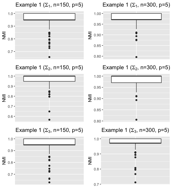
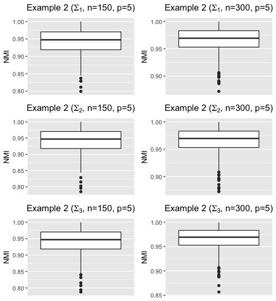
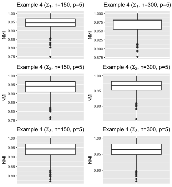
Figure 1: The normalized mutual information (NMI) in Example 1, 2 and 4, where $n=150,300$, and $p=5$.

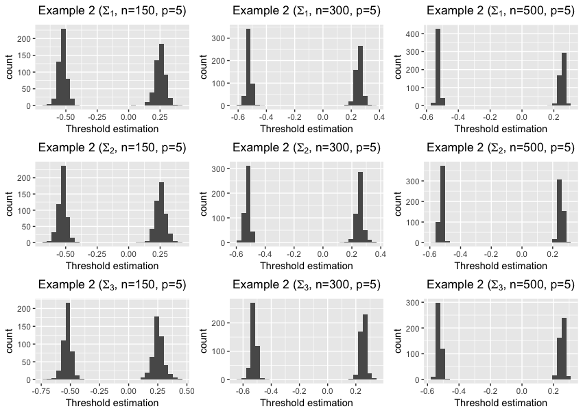
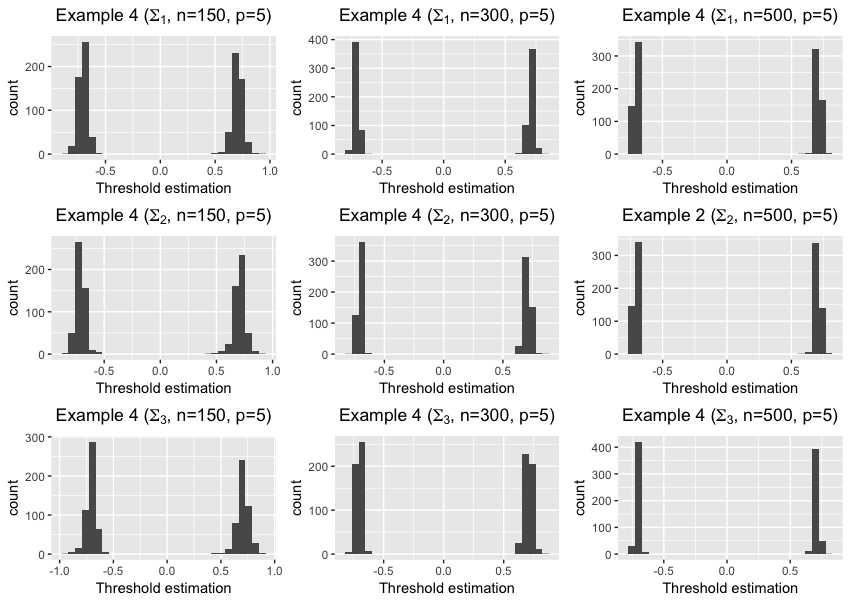
Figure 2: Histograms of the estimated thresholds for Example $2$ and $4$. The true values are $(-0.524,0.253)$ and $(-\sqrt{2}/2,\sqrt{2}/2)$ for Example $2$ and $4$ respectively.

Table 6: Estimation performance for the threshold estimation for Example $2$. Bias is the average of estimated parameter minus the true value. SD is the empirical standard deviation. RMSE refers to the relative mean squared errors.

			$a_{1}$			$a_{2}$
			Bias	SD	RMSE	Bias	SD	RMSE
$\Sigma_{ij}=\bm{1}_{\{i=j\}}$	$n=150$	$p=5$	0.001	0.034	0.033	0.001	0.041	0.041
		$p=20$	0.005	0.035	0.035	-0.003	0.047	0.047
	$n=300$	$p=5$	-0.001	0.017	0.017	0.001	0.022	0.022
		$p=20$	0.001	0.019	0.019	0.001	0.021	0.021
	$n=500$	$p=5$	0.001	0.009	0.010	0.001	0.013	0.013
		$p=20$	0.001	0.011	0.011	0.001	0.012	0.012
$\Sigma_{ij}=0.5^{|i-j|}$	$n=150$	$p=5$	0.001	0.033	0.033	-0.001	0.041	0.041
		$p=20$	0.008	0.044	0.045	-0.006	0.048	0.048
	$n=300$	$p=5$	-0.001	0.017	0.017	0.001	0.024	0.024
		$p=20$	0.001	0.019	0.019	-0.001	0.022	0.022
	$n=500$	$p=5$	-0.001	0.010	0.010	0.001	0.014	0.014
		$p=20$	-0.001	0.010	0.010	-0.001	0.012	0.012
$\Sigma_{ij}=1-0.5\cdot\bm{1}_{\{i\neq j\}}$	$n=150$	$p=5$	0.003	0.037	0.038	-0.001	0.049	0.049
		$p=20$	0.012	0.047	0.049	-0.007	0.049	0.050
	$n=300$	$p=5$	-0.001	0.021	0.021	0.002	0.022	0.022
		$p=20$	0.002	0.021	0.021	-0.001	0.025	0.025
	$n=500$	$p=5$	-0.001	0.012	0.012	-0.001	0.015	0.015
		$p=20$	-0.001	0.013	0.013	0.001	0.015	0.015

Table 7: Estimation performance for the change-plane estimation for Example $2$. Bias is the average of estimated parameter minus the true value. SD is the empirical standard deviation. RMSE refers to the relative mean squared errors.

$\theta_{1}$ $\theta_{2}$ $\theta_{3}$ Bias SD RMSE Bias SD RMSE Bias SD RMSE $\Sigma_{ij}=\bm{1}_{\{i=j\}}$ $n=150$ $p=5$ 0.001 0.018 0.017 0.001 0.027 0.027 0.001 0.020 0.020 $p=20$ 0.001 0.017 0.017 0.000 0.027 0.026 0.001 0.020 0.020 $n=300$ $p=5$ -0.001 0.009 0.009 0.001 0.013 0.013 0.001 0.011 0.011 $p=20$ -0.001 0.011 0.011 -0.001 0.014 0.014 0.001 0.012 0.012 $n=500$ $p=5$ 0.001 0.006 0.006 0.001 0.008 0.008 0.001 0.006 0.006 $p=20$ 0.001 0.006 0.006 0.001 0.008 0.008 0.001 0.006 0.006 $\Sigma_{ij}=0.5^{|i-j|}$ $n=150$ $p=5$ 0.001 0.020 0.020 -0.003 0.028 0.029 -0.001 0.022 0.022 $p=20$ 0.004 0.024 0.025 0.001 0.032 0.032 -0.003 0.028 0.029 $n=300$ $p=5$ 0.001 0.010 0.010 -0.001 0.014 0.014 0.001 0.011 0.011 $p=20$ 0.001 0.011 0.011 0.001 0.014 0.014 0.001 0.012 0.012 $n=500$ $p=5$ 0.001 0.007 0.007 0.001 0.009 0.009 0.001 0.007 0.007 $p=20$ 0.001 0.007 0.007 0.001 0.008 0.008 0.001 0.007 0.007 $\Sigma_{ij}=1-0.5\cdot\bm{1}_{\{i\neq j\}}$ $n=150$ $p=5$ 0.001 0.028 0.028 -0.002 0.028 0.028 0.001 0.032 0.032 $p=20$ 0.003 0.046 0.046 -0.007 0.036 0.037 -0.002 0.046 0.046 $n=300$ $p=5$ 0.001 0.016 0.016 -0.001 0.016 0.016 0.001 0.018 0.018 $p=20$ 0.001 0.016 0.016 0.001 0.017 0.017 0.001 0.018 0.018 $n=500$ $p=5$ 0.001 0.010 0.010 0.001 0.009 0.009 0.001 0.011 0.011 $p=20$ 0.001 0.009 0.009 0.001 0.009 0.009 0.001 0.010 0.010

Table 8: Estimation performance for the threshold estimation for Example $4$. Bias is the average of estimated parameter minus the true value. SD is the empirical standard deviation. RMSE refers to the relative mean squared errors.

			$a_{1}$			$a_{2}$
			Bias	SD	RMSE	Bias	SD	RMSE
$\Sigma_{ij}=\bm{1}_{\{i=j\}}$	$n=150$	$p=5$	-0.001	0.040	0.040	0.002	0.049	0.049
		$p=20$	0.006	0.049	0.05	0.001	0.046	0.046
	$n=300$	$p=5$	-0.002	0.019	0.019	0.001	0.024	0.024
		$p=20$	0.001	0.020	0.020	0.001	0.025	0.025
	$n=500$	$p=5$	0.001	0.012	0.012	0.001	0.017	0.017
		$p=20$	0.001	0.011	0.011	0.001	0.014	0.014
$\Sigma_{ij}=0.5^{|i-j|}$	$n=150$	$p=5$	0.003	0.041	0.042	0.004	0.055	0.055
		$p=20$	0.014	0.050	0.052	0.006	0.048	0.049
	$n=300$	$p=5$	0.002	0.020	0.020	0.001	0.028	0.028
		$p=20$	0.001	0.022	0.022	-0.001	0.028	0.028
	$n=500$	$p=5$	0.001	0.012	0.012	0.001	0.017	0.017
		$p=20$	0.001	0.013	0.013	0.001	0.017	0.017
$\Sigma_{ij}=1-0.5\cdot\bm{1}_{\{i\neq j\}}$	$n=150$	$p=5$	0.001	0.047	0.047	0.002	0.058	0.058
		$p=20$	0.012	0.057	0.058	0.005	0.065	0.065
	$n=300$	$p=5$	0.001	0.024	0.024	0.001	0.030	0.030
		$p=20$	0.001	0.026	0.026	-0.001	0.026	0.026
	$n=500$	$p=5$	0.001	0.014	0.014	0.001	0.018	0.018
		$p=20$	-0.001	0.014	0.014	0.001	0.018	0.018

Table 9: Estimation performance for the change-plane estimation for Example $4$. Bias is the average of estimated parameter minus the true value. SD is the empirical standard deviation. RMSE refers to the relative mean squared errors.

$\theta_{1}$ $\theta_{2}$ $\theta_{3}$ Bias SD RMSE Bias SD RMSE Bias SD RMSE $\Sigma_{ij}=\bm{1}_{\{i=j\}}$ $n=150$ $p=5$ 0.001 0.021 0.021 0.001 0.029 0.029 0.001 0.026 0.026 $p=20$ 0.001 0.024 0.024 0.001 0.040 0.040 0.001 0.029 0.029 $n=300$ $p=5$ 0.001 0.011 0.011 -0.001 0.015 0.015 0.001 0.012 0.012 $p=20$ 0.001 0.011 0.011 0.001 0.017 0.017 0.001 0.013 0.013 $n=500$ $p=5$ 0.001 0.007 0.007 -0.001 0.010 0.010 0.001 0.008 0.008 $p=20$ 0.001 0.006 0.006 0.001 0.010 0.010 0.001 0.007 0.007 $\Sigma_{ij}=0.5^{|i-j|}$ $n=150$ $p=5$ 0.001 0.024 0.024 0.001 0.032 0.032 0.001 0.026 0.026 $p=20$ 0.002 0.030 0.030 0.001 0.040 0.040 0.001 0.031 0.031 $n=300$ $p=5$ 0.001 0.011 0.011 0.001 0.016 0.016 0.001 0.012 0.012 $p=20$ -0.001 0.011 0.011 -0.001 0.016 0.016 0.001 0.013 0.013 $n=500$ $p=5$ 0.001 0.007 0.007 0.001 0.010 0.010 0.001 0.007 0.008 $p=20$ 0.001 0.007 0.007 0.001 0.010 0.010 0.001 0.008 0.008 $\Sigma_{ij}=1-0.5\cdot\bm{1}_{\{i\neq j\}}$ $n=150$ $p=5$ 0.003 0.032 0.032 -0.003 0.034 0.034 -0.002 0.037 0.037 $p=20$ 0.002 0.035 0.035 -0.003 0.041 0.041 0.001 0.039 0.039 $n=300$ $p=5$ 0.001 0.018 0.018 0.001 0.017 0.017 -0.001 0.019 0.019 $p=20$ -0.001 0.017 0.017 -0.001 0.018 0.018 0.001 0.019 0.019 $n=500$ $p=5$ 0.001 0.01 0.010 0.001 0.010 0.010 0.001 0.010 0.010 $p=20$ 0.001 0.011 0.011 0.001 0.010 0.010 0.001 0.012 0.012

Table 6 and Table 8 summarize the estimation performance of the estimated thresholds $\bm{a}$ for the cases with correct estimation of $\hat{s}=s$ in Examples $2$ and $4$. In both examples, the estimations are of small bias and mean squared error. In fact we note that the jumps at the two change points are $\|\bm{\delta}_{1}\|^{2}=4$ and $\|\bm{\delta}_{2}\|^{2}=2$, respectively, under both equal and unequal group size situation. In general it is easier for our methods to estimate the greater jump. In addition, we report the bias and the SD of estimated change plane parameter $\bm{\theta}$ in Table 7 and Table 9 for Examples 2 and 4 respectively. From the tables, we can conclude that our estimation performs very well for estimating the change plane parameters.

Finally we report the estimation performance of the sparse regression coefficients $\hat{\bm{\gamma}}^{*}$ using boxplots in Figure 3. The estimated coefficients are all consistent to the true parameter values. The zero coefficients $\gamma_{j}$, $j=8,9,13,16,17,18$, can be accurately identified by our method. Table 10 also shows the number of correctly selected zeros and incorrectly selected zeros in $\hat{\bm{\gamma}}^{*}$, suggesting a satisfactory variable selection performance.

Table 10: Variable selection results for Example $2$ and Example $4$ in case of $p=5$. In these cases $6$ coefficients are zero. Correct and Incorrect refer to the average number of estimated zero coefficients corresponding to the true zero and non-zero coefficients, respectively.

		Avg. no. of $0$ coefficients
		Example 2		Example 4
		Correct	Incorrect	Correct	Incorrect
$\Sigma_{ij}=\bm{1}_{\{i=j\}}$	$n=150$	5.871	0.088	5.649	0.365
	$n=300$	5.971	0	5.935	0.010
$\Sigma_{ij}=0.5^{|i-j|}$	$n=150$	5.738	0.298	5.357	0.900
	$n=300$	5.948	0.008	5.658	0.077
$\Sigma_{ij}=1-0.5\cdot\bm{1}_{\{i\neq j\}}$	$n=150$	5.869	0.246	5.706	0.554
	$n=300$	5.970	0.002	5.917	0.021

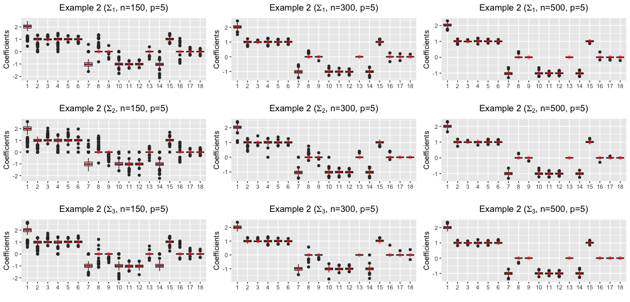
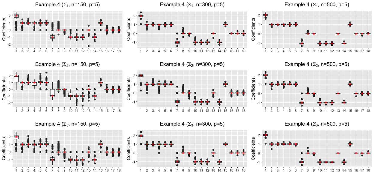
Figure 3: Box plots of estimated coefficients $\hat{\bm{\gamma}}^{*}$ for Example $2$ and $4$ with three different structures of $\Sigma$. “$*$”s are the true values.

5 Application to Real Data

5.1 Bovine Collagen Clinical Trial (BCCT)

We illustrate our methods using clinical data from a 3-year NIH-sponsored randomized Bovine Collagen Trial for Scleroderma patients conducted at 12 centers in the USA which contains 297 samples (Postlethwaite et al. 2008; Li and Wong 2009). Patients were randomized to receive oral native collagen at a dose of 500 $\mu\textnormal{g/day}$ or a placebo. They were evaluated clinically by the Modified Rodnan Skin Score (MRSS) (the primary outcome variable), disability index of the Health Assessment Questionnaire (HAQ), patient’s global assessment, patients pain assessment and physicians global assessment. To implement the proposed method, we consider $11$ predictor variables: $X_{1}=$ haq (health assessment questionnaire); $X_{2}=$ pga (patient self assessment of disease progression); $X_{3}=$ dlcop (lung performance measurement 3); $X_{4}=$ fvcp (lung performance measurement 1); $X_{5}=$ over (disease progression); $X_{6}=$ pain (index of pain); $X_{7}=$ fev1p (lung performance measurement 2); $X_{8}=$ durdis (duration of disease); $X_{9}=$ age (in years) $X_{10}=$ ethnic ($0=$ hispanic, $1=$ non-hispanic); $X_{11}=$ sex ($0=$ female, $1=$ male). Variables are standardized with mean zero and unit variance.

We first fit a linear regression model with $\bm{X}_{i}=(1,X_{i1},\ldots,X_{i,11})^{\mathrm{T}}$ without considering subgroups, and denote $\hat{\bm{\beta}}^{\textup{ols}}$ the OLS estimation. Then, for subgroup identification, we choose $\bm{Z}_{i}=(X_{i1},X_{i2},X_{i3})^{\mathrm{T}}$ to be the threshold variables and fit the multiple threshold change-plane model. The tuning parameters in (10) were chosen via generalized cross-validation (GCV). We detect one change by our method with the estimated threshold $\hat{a}^{*}=-0.125$ and the change-plane parameter $\hat{\bm{\theta}}^{*}=(0.801,-0.206,0.562)^{\mathrm{T}}$. The two subgroup sizes are $139$ and $155$ respectively and we report the estimated coefficients $\bm{\beta}$ and $\bm{\delta}$ in Table 11 with their standard errors (S.E.), and the $p$-values for testing the significance of the coefficients.

We compared our MCPL models with the multiple change-points (MCPT) models proposed in Li and Jin (2017) with single thresholding covariate being $X_{1}$, $X_{2}$, $X_{3}$ respectively and also with a version of MCPL with equally weighted plane variable $\bm{Z}_{i}=(X_{i1}+X_{i2}+X_{i3})/3$ (E-MCPL). From Table 12, we can see that these methods yield quite different subgroups and our proposed MCPL has the smallest mean squared error for predicting the MRSS response. In particular, we plot the scatter plots of predicted MRSS versus observed MRSS in Figure 4. One can see that the prediction from MCPL is less variable than the other methods.

To gain more understanding of the groups, we summarize the means of all covariates for the detected subgroups in Figure 5. Eyeballing the plots we can see that the mean difference of all the covariates between the two subgroups detected by MCPL are quite different compared to the other methods. We also plot the kernel density estimation of the thresholding variable ${\bf Z}^{T}\hat{\bm{\theta}}$ for all methods in Figure 6.

Table 11: Estimated results for Bovine Collagen Clinical Trial (BCCT), along with standard errors (S.E.) and P-values. $X_{1}=$ haq; $X_{2}=$ pga; $X_{3}=$ dlcop; $X_{4}=$ fvcp; $X_{5}=$ over; $X_{6}=$ pain; $X_{7}=$ fev1p; $X_{8}=$ durdis; $X_{9}=$ age $X_{10}=$ ethnic (non-hispanic); $X_{11}=$ sex (male).

	$\bm{\beta}$			$\bm{\delta}$			$\bm{\beta}^{\textup{ols}}$
Covariates	Coef.	S.E.	P-value	Coef.	S.E.	P-value	Coef.	S.E.	P-value
Intercept	0.022	0.104	0.830	-0.525	0.238	0.028	-0.383	0.188	0.042
$X_{1}$	0	-	-	0.443	0.125	$<0.001$	0.220	0.065	$<0.001$
$X_{2}$	0.416	0.057	$<0.001$	0	-	-	0.369	0.059	$<0.001$
$X_{3}$	0.332	0.102	0.001	-0.261	0.131	0.048	0.113	0.058	0.051
$X_{4}$	0.124	0.081	0.127	0	-	-	0.118	0.086	0.170
$X_{5}$	-0.296	0.128	0.022	0.547	0.173	0.002	0.065	0.092	0.480
$X_{6}$	0.245	0.122	0.045	-0.602	0.160	$<0.001$	-0.095	0.087	0.276
$X_{7}$	-0.322	0.099	0.001	0.307	0.111	0.006	-0.121	0.084	0.153
$X_{8}$	-0.187	0.068	0.006	0.313	0.105	0.003	-0.063	0.055	0.251
$X_{9}$	-0.104	0.050	0.037	0	-	-	-0.115	0.053	0.031
$X_{10}$	0	-	-	0.367	0.209	0.080	0.386	0.195	0.049
$X_{11}$	-0.376	0.172	0.029	0.771	0.247	0.002	0.138	0.130	0.287

Table 12: Estimated Comparison for Bovine Collagen Clinical Trial (BCCT). MCPL stands for multiple change-plane, MCPT-$X_{1}$, MCPT-$X_{2}$, MCPT-$X_{3}$ stands for the MCPT method with threshold $X_{1}$, $X_{2}$ and $X_{3}$ respectively, E-MCPL stands for multiple change plane with equal weight and OLS stands for the ordinary least square estimate.

Model	MSE	$\hat{s}$	threshod $\hat{a}$	Group Sizes
MCPL	0.613	1	$-0.125$	$138:156$
MCPT-$X_{1}$	0.695	1	$-0.695$	$72:222$
MCPT-$X_{2}$	0.672	2	$(-0.079,0.916)$	$150:81:63$
MCPT-$X_{3}$	0.786	1	$-0.996$	$42:252$
E-MCPL	0.707	2	$(-0.259,0.029)$	$103:51:140$
OLS	0.739	0	-	-

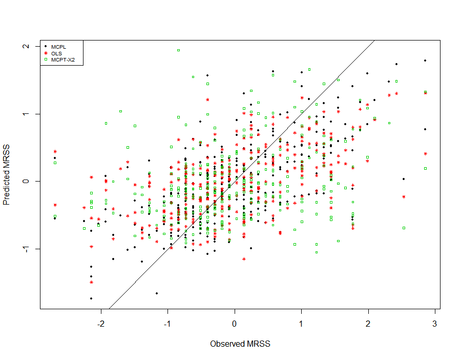
Figure 4: The scatter plot of the fitted $Y$ by each method for BCCT data. MCPL stands for multiple threshold change-plane, MCPT-$X_{2}$, stands for the MCPT method with threshold variable $X_{2}$ and OLS stands for the ordinary least square estimate.

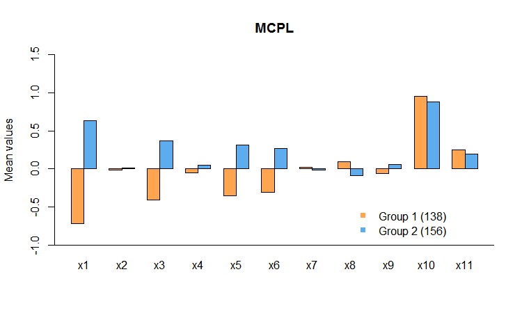
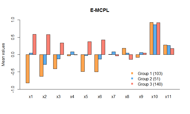
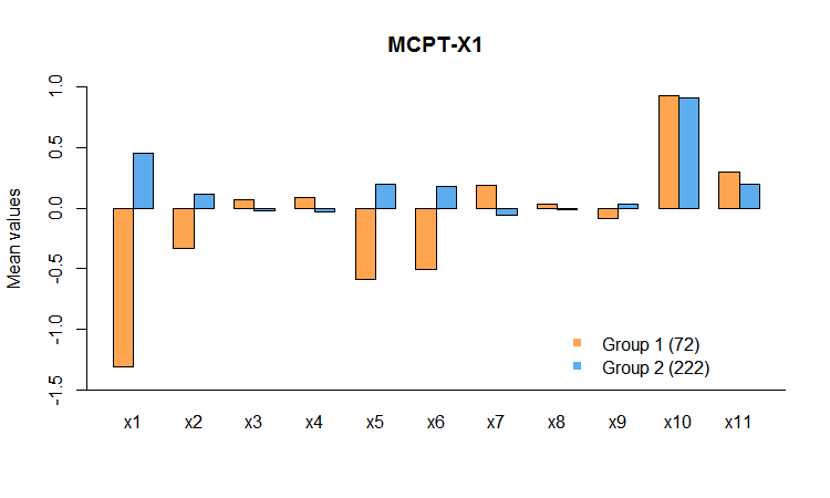
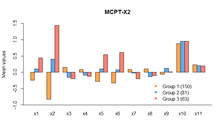
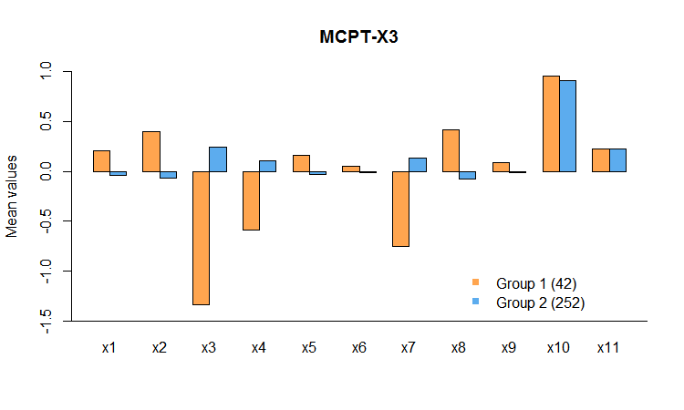
Figure 5: The mean value of predoctors for different detected subgroups for BCCT data. MCPL stands for multiple change-plane model, E-MCPL stands for multiple change plane with equal weight, MCPT-$X_{1}$, MCPT-$X_{2}$, MCPT-$X_{3}$ stands for the MCPT method with threshold $X_{1}$, $X_{2}$ and $X_{3}$ respectively. $X_{1}=$ haq; $X_{2}=$ pga; $X_{3}=$ dlcop; $X_{4}=$ fvcp; $X_{5}=$ over; $X_{6}=$ pain; $X_{7}=$ fev1p; $X_{8}=$ durdis; $X_{9}=$ age $X_{10}=$ ethnic (non-hispanic); $X_{11}=$ sex (male). Group sizes are given in parentheses.

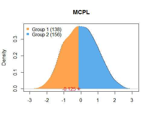
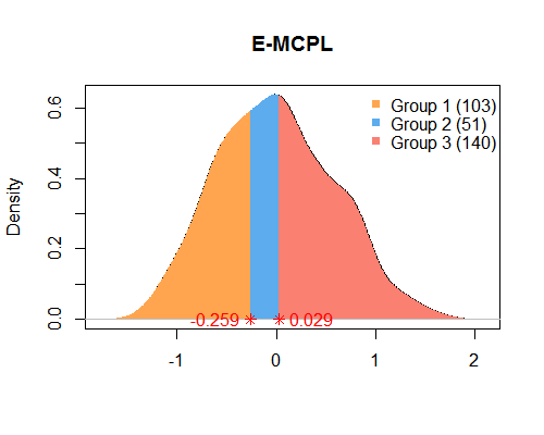
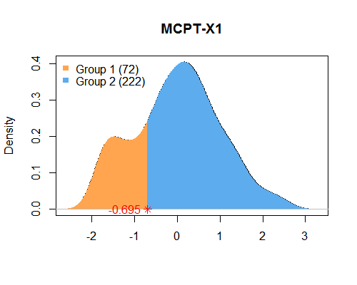
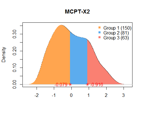
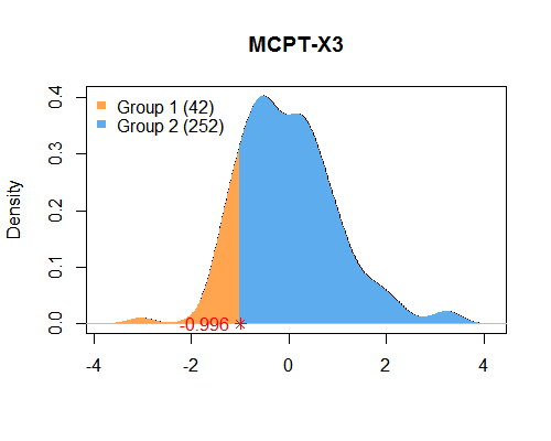
Figure 6: The density plots of thresholding varibles estimated by each method for BCCT data, the red mark points in x-axis disply the cut-off points. MCPL stands for multiple change-plane, SCPL stands for single change-plane, E-MCPL stands for multiple change plane with equal weight, MCPT-$X_{1}$, MCPT-$X_{2}$, MCPT-$X_{3}$ stands for the MCPT method with threshold $X_{1}$, $X_{2}$ and $X_{3}$ respectively. Group sizes are given in parentheses.

5.2 AIDS Clinical Trials

We apply our method to the AIDS Clinical Trials Group Study 175 (ACTG175), which contains 2139 HIV-infected subjects. This randomized clinical trial compares zidovudine (ZDV) monotherapy (treatment 0) with other three therapies including ZDV and didanosine (ddI) (treatment 1), ZDV and zalcitabine (zal) (treatment 2), and ddI monotherapy (treatment 3) in adults infected with the human immunodeficiency virus type I (Tsiatis et al. 2008; Lu et al. 2013). Our interest is to conduct subgroup analysis to produce more satisfactory predicted value of CD4 counts (cells/mm³) at $20\pm 5$ weeks. We consider the following covariates: $X_{1}=$ hemophilia (0 =no, 1 =yes); $X_{2}=$ gender (0 =female, 1 =male); $X_{3}=$ CD4 counts at baseline; $X_{4}=$ antiretroviral history (0 =naive, 1 =experienced); $X_{5}=$ age (years); $X_{6}=$ weight (kg); $X_{7}=$ Karnofsky score; $X_{8}=$ CD8 counts at baseline; $X_{9}=$ homosexual activity (0 =no, 1 =yes); $X_{10}=$ history of intravenous drug use (0 =no, 1 =yes); $X_{11}=$ race (0 =white, 1 =white); $X_{12}=$ symptomatic status (0 =asymptomatic, 1 =symptomatic) and $X_{13}=$ treatment arm (0=zidovudine, 1=zidovudine and didanosine, 2=zidovudine and zalcitabine, 3=didanosine).

We first fit a linear regression model with $\bm{X}_{i}=(1,X_{i1},\ldots,X_{i,14})^{\mathrm{T}}$ without subgroups, and denote $\hat{\bm{\beta}}^{\textup{ols}}$ the OLS estimation. We then fit the MCPL model (5), and choose $\bm{Z}_{i}=(X_{i1},X_{i2},X_{i3},X_{i4},X_{i5})^{\mathrm{T}}$ as the threshold variables. Similarly, the tuning parameters in (10) were chosen via the GCV. The estimated change-plane parameter $\hat{\bm{\theta}}^{*}=(-0.268,-0.199,0.876,-0.268,0.223)^{\mathrm{T}}$. We detect two change planes by our method where the estimated threshold locations are $\hat{\bm{a}}^{*}=(-0.309,0.201)^{\mathrm{T}}$, thus producing three subgroups with group sizes $1162$, $394$, and $583$ respectively. Table 13 reports the estimated coefficients $\bm{\beta}$ and $\bm{\delta}$, their standard errors (S.E.), and the $p$-values for testing the significance of the coefficients.

We also compared the prediction performance of our MCPL models with the single-threshold change-plane (SCPL) models (1), with the multiple change-points (MCPT) models proposed in Li and Jin (2017) with single threshold covariate being $X_{3}$ and $X_{5}$ respectively and also with a version of MCPL with equally weighted plane multiple variables $\bm{Z}_{i}=(X_{1}+\cdots+X_{5})/5$ (E-MCPL). In this case, $X_{1}$, $X_{2}$ and $X_{4}$ are not continuous and cannot be applied in MCPT model. The MSE results from all these methods are summarized in table 14 and we can see that MCPL achieves the smallest MSE. Furthermore, we display the scatter plots of predicted CD4 counts versus observed CD4 counts in Figure 7. We can draw similar conclusion as in the first example. To study the subgroups, we summarize the means of all the covariates for the subgroup in Figure 8. We also plot the kernel density plots of the thresholding variables for all methods in Figure 9.

Table 13: Estimated results for AIDS Clinical Trials Group Study 175 (ZDV vs. the other three treatments), along with standard errors (S.E.) and P-values by t test. $X_{0}=$ Intercept; $X_{1}=$ hemophilia (yes); $X_{2}=$ gender (male); $X_{3}=$ CD4 counts at baseline; $X_{4}=$ antiretroviral history (experienced); $X_{5}=$ age; $X_{6}=$ weight; $X_{7}=$ Karnofsky score; $X_{8}=$ CD8 counts at baseline; $X_{9}=$ homosexual activity (yes); $X_{10}=$ history of intravenous drug use (yes); $X_{11}=$ race (white); $X_{12}=$ symptomatic status (symptomatic), $X_{13}=$ treatment arm¹ (zidovudine and didanosine), $X_{14}=$ treatment arm² (zidovudine and zalcitabine) and $X_{15}=$ treatment arm³ (didanosine).

	$\bm{\beta}$			$\bm{\delta}_{1}$			$\bm{\delta}_{2}$			$\bm{\beta}^{\textup{ols}}$
	Coef.	S.E.	P-value	Coef.	S.E.	P-value	Coef.	S.E.	P-value	Coef.	S.E.	P-value
$X_{0}$	-0.087	0.059	0.143	0.171	0.078	0.029	0.286	0.092	0.002	-0.001	0.061	0.981
$X_{1}$	-0.169	0.062	0.007	0	-	-	0	-	-	-0.184	0.080	0.021
$X_{2}$	0	-	-	0	-	-	0	-	-	-0.032	0.066	0.632
$X_{3}$	0.568	0.041	$<0.001$	0	-	-	-0.269	0.058	$<0.001$	0.571	0.017	$<0.001$
$X_{4}$	-0.247	0.035	$<0.001$	0	-	-	0	-	-	-0.281	0.035	$<0.001$
$X_{5}$	0	-	-	-0.117	0.025	$<0.001$	0	-	-	0.021	0.017	0.234
$X_{6}$	0	-	-	0	-	-	0	-	-	-0.003	0.018	0.846
$X_{7}$	0.085	0.021	$<0.001$	-0.233	0.047	$<0.001$	0.187	0.055	0.001	0.040	0.017	0.019
$X_{8}$	-0.109	0.024	$<0.001$	0.085	0.034	0.012	0	-	-	-0.066	0.017	$<0.001$
$X_{9}$	0	-	-	-0.064	0.057	0.257	0	-	-	0.003	0.059	0.957
$X_{10}$	0.092	0.058	0.111	0	-	-	-0.167	0.109	0.128	0.052	0.052	0.319
$X_{11}$	-0.101	0.043	0.020	0	-	-	-0.128	0.083	0.123	-0.128	0.040	0.002
$X_{12}$	-0.135	0.055	0.015	0.103	0.120	0.390	-0.110	0.145	0.450	-0.130	0.045	0.004
$X_{13}$	0.452	0.061	$<0.001$	0.164	0.107	0.125	-0.124	0.121	0.309	0.488	0.048	$<0.001$
$X_{14}$	0.251	0.062	$<0.001$	0.008	0.086	0.927	0	-	-	0.252	0.048	$<0.001$
$X_{15}$	0.228	0.052	$<0.001$	0	-	-	0.261	0.096	0.007	0.294	0.047	$<0.001$

Table 14: Estimated Comparison for AIDS Clinical Trials Group Study 175 data (ZDV vs. the other three treatments). MCPL stands for multiple change-plane, SCPL stands for single change-plane, MCPT-$X_{3}$, MCPT-$X_{5}$stands for the MCPT method with threshold $X_{3}$ and $X_{5}$ respectively, E-MCPL stands for multiple change plane with equal weight and OLS stands for the ordinary least square estimate.

Method	MSE	$\hat{s}$	Threshold $\hat{a}$	Group Sizes
MCPL	0.567	2	$(-0.309,0.201)$	$1162:394:583$
SCPL	0.578	1	0	$489:1650$
MCPT-$X_{3}$	0.575	2	$(-1.758,1.210)$	$21:1889:229$
MCPT-$X_{5}$	0.595	0	-	-
E-MCPL	0.595	0	-	-
OLS	0.595	0	-	-

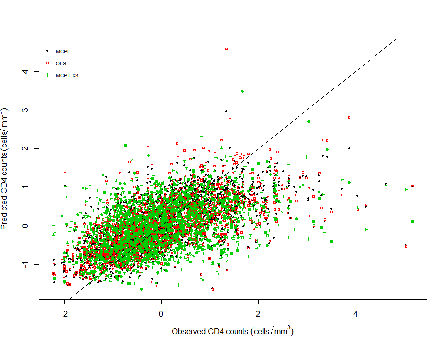
Figure 7: The scatter plot of the fitted $Y$ by each method for ACTG 175 data. MCPL stands for multiple change-plane, MCPT-$X_{3}$, stands for the MCPT method with threshold $X_{3}$ and OLS stands for the ordinary least square estimate.

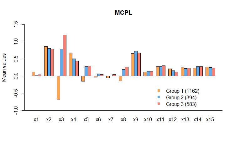
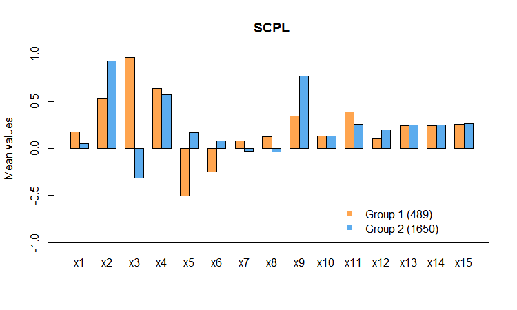
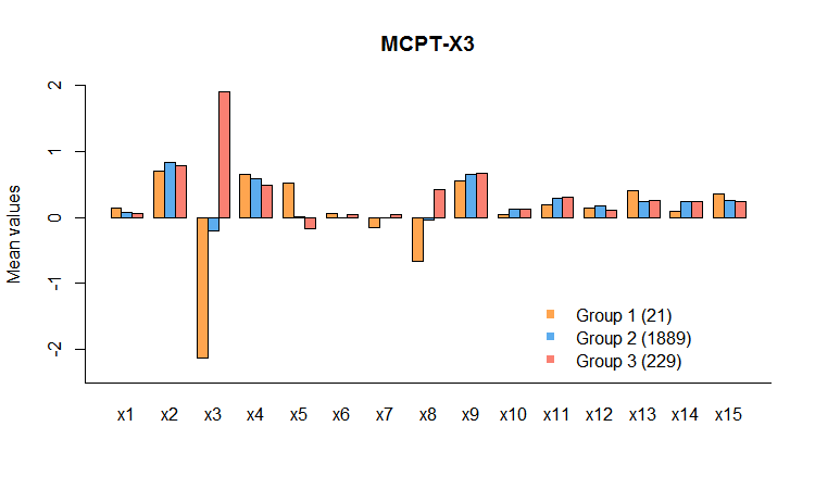
Figure 8: The mean value of predoctors for different detected subgroups for ACTG 175 data. MCPL stands for multiple change-plane, SCPL stands for single change-plane, MCPT-$X_{3}$ stands for the MCPT method with threshold $X_{3}$. $X_{1}=$ hemophilia (yes); $X_{2}=$ gender (male); $X_{3}=$ CD4 counts at baseline; $X_{4}=$ antiretroviral history (experienced); $X_{5}=$ age; $X_{6}=$ weight; $X_{7}=$ Karnofsky score; $X_{8}=$ CD8 counts at baseline; $X_{9}=$ homosexual activity (yes); $X_{10}=$ history of intravenous drug use (yes); $X_{11}=$ race (white); $X_{12}=$ symptomatic status (symptomatic), $X_{13}=$ treatment arm¹ (zidovudine and didanosine), $X_{14}=$ treatment arm² (zidovudine and zalcitabine) and $X_{15}=$ treatment arm³ (didanosine). Group sizes are given in parentheses.

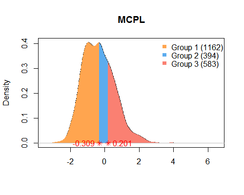
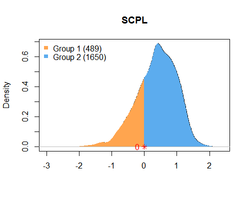
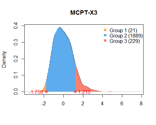
Figure 9: The density plots of thresholding varibles estimated by each method for ACTG 175 data, the red mark points in x-axis disply the cut-off points. MCPL stands for multiple change-plane, SCPL stands for single change-plane, MCPT-$X_{3}$ stands for the MCPT method with threshold $X_{3}$. Group sizes are given in parentheses.

6 Discussion

In our theoretical results, we allow the coefficients of the covariates to be sparse, but require their dimension to be much smaller than $n$. A high or ultra-high dimensional situation can be further investigated (Shi et al. 2017). Our proposed method can be extended to other models including generalized linear models and hazard regression models to incorporate non-Gaussian response variables. Although these extensions appear to be conceptually straightforward, it is a nontrivial task to develop computational algorithms and establish theoretical properties in these more complicated models.

Supplementary Materials

The supplementary materials contain technical proofs for Theorems 1-3.

References

- Ana and Jain (2003) Ana, L. and A. K. Jain (2003). Robust data clustering. In Computer Vision and Pattern Recognition, 2003. Proceedings. 2003 IEEE Computer Society Conference on, Volume 2, pp. II–II. IEEE.
- Bai (1997) Bai, J. (1997). Estimation of a change point in multiple regression models. Review of Economics and Statistics 79(4), 551–563.
- Breheny and Huang (2011) Breheny, P. and J. Huang (2011). Coordinate descent algorithms for nonconvex penalized regression, with applications to biological feature selection. The Annals of Applied Statistics 5(1), 232–253.
- Cai et al. (2011) Cai, T., L. Tian, P. H. Wong, and L. Wei (2011). Analysis of randomized comparative clinical trial data for personalized treatment selections. Biostatistics 12(2), 270–282.
- Chen et al. (2017) Chen, S., L. Tian, T. Cai, and M. Yu (2017). A general statistical framework for subgroup identification and comparative treatment scoring. Biometrics 73(4), 1199–1209.
- Fan et al. (2017) Fan, A., R. Song, and W. Lu (2017). Change-plane analysis for subgroup detection and sample size calculation. Journal of the American Statistical Association, 1–10.
- Fan et al. (2017) Fan, C., W. Lu, R. Song, and Y. Zhou (2017). Concordance-assisted learning for estimating optimal individualized treatment regimes. Journal of the Royal Statistical Society: Series B (Statistical Methodology) 79(5), 1565–1582.
- Fan and Li (2001) Fan, J. and R. Li (2001). Variable selection via nonconcave penalized likelihood and its oracle properties. Journal of the American statistical Association 96(456), 1348–1360.
- Fan and Tang (2013) Fan, Y. and C. Y. Tang (2013). Tuning parameter selection in high dimensional penalized likelihood. Journal of the Royal Statistical Society: Series B (Statistical Methodology) 75(3), 531–552.
- Foster et al. (2011) Foster, J., J. Taylor, and S. Ruberg (2011). Subgroup identification from randomized clinical trial data. Statistics in Medicine 30, 2867–2880.
- Goldberg and Kosorok (2012) Goldberg, Y. and M. R. Kosorok (2012). Q-learning with censored data. Annals of statistics 40(1), 529.
- Golub and Pereyra (2003) Golub, G. and V. Pereyra (2003). Separable nonlinear least squares: the variable projection method and its applications. Inverse problems 19(2), R1.
- Gonzalo and Pitarakis (2002) Gonzalo, J. and J.-Y. Pitarakis (2002). Estimation and model selection based inference in single and multiple threshold models. Journal of Econometrics 110(2), 319–352.
- Hansen (2000) Hansen, B. E. (2000). Sample splitting and threshold estimation. Econometrica 68(3), 575–603.
- Horowitz (1992) Horowitz, J. L. (1992). A smoothed maximum score estimator for the binary response model. Econometrica: journal of the Econometric Society, 505–531.
- Horowitz (2002) Horowitz, J. L. (2002). Bootstrap critical values for tests based on the smoothed maximum score estimator. Journal of Econometrics 111(2), 141–167.
- Jiang et al. (2017) Jiang, R., W. Lu, R. Song, and M. Davidian (2017). On estimation of optimal treatment regimes for maximizing t-year survival probability. Journal of the Royal Statistical Society: Series B (Statistical Methodology) 79(4), 1165 C1185.
- Jin et al. (2013) Jin, B., X. Shi, and Y. Wu (2013). A novel and fast methodology for simultaneous multiple structural break estimation and variable selection for nonstationary time series models. Statistics and Computing 23(2), 221–231.
- Johnson and Strawderman (2009) Johnson, L. M. and R. L. Strawderman (2009). Induced smoothing for the semiparametric accelerated failure time model: asymptotics and extensions to clustered data. Biometrika 96(3), 577–590.
- Kourtellos et al. (2016) Kourtellos, A., T. Stengos, and C. M. Tan (2016). Structural threshold regression. Econometric Theory 32(4), 827–860.
- Lee et al. (2016) Lee, S., M. H. Seo, and Y. Shin (2016). The lasso for high dimensional regression with a possible change point. Journal of the Royal Statistical Society: Series B (Statistical Methodology) 78(1), 193–210.
- Li and Ling (2012) Li, D. and S. Ling (2012). On the least squares estimation of multiple-regime threshold autoregressive models. Journal of Econometrics 167(1), 240–253.
- Li and Jin (2017) Li, J. and B. Jin (2017). Multi-threshold accelerate failure time model. The Annals of Statistics, (in press).
- Li and Wong (2009) Li, J. and W. K. Wong (2009). A semi-parametric analysis for identifying scleroderma patients responsive to an anti-fibrotic agent. Contemporary clinical trials 30(2), 105–113.
- Loh (2002) Loh, W. (2002). Regression trees with unbiased variable selection and interaction detection. Statistica Sinica 12, 361–386.
- Lu et al. (2013) Lu, W., H. H. Zhang, and D. Zeng (2013). Variable selection for optimal treatment decision. Statistical methods in medical research 22(5), 493–504.
- Messenger and Mandell (1972) Messenger, R. and L. Mandell (1972). A modal search technique for predictive nominal scale multivariate analysis. Journal of the American Statistical Association 67, 768–772.
- Morgan and Sonquist (1963) Morgan, J. and J. Sonquist (1963). Problems in the analysis of survey data and a proposal. Journal of the American Statistical Association 58, 415–434.
- Murphy (2003) Murphy, S. A. (2003). Optimal dynamic treatment regimes. Journal of the Royal Statistical Society: Series B (Statistical Methodology) 65(2), 331–355.
- Postlethwaite et al. (2008) Postlethwaite, A. E., W. K. Wong, P. Clements, S. Chatterjee, B. J. Fessler, A. H. Kang, J. Korn, M. Mayes, P. A. Merkel, J. A. Molitor, et al. (2008). A multicenter, randomized, double-blind, placebo-controlled trial of oral type i collagen treatment in patients with diffuse cutaneous systemic sclerosis: I. oral type i collagen does not improve skin in all patients, but may improve skin in late-phase disease. Arthritis & Rheumatology 58(6), 1810–1822.
- Qian and Murphy (2011) Qian, M. and S. A. Murphy (2011). Performance guarantees for individualized treatment rules. Annals of statistics 39(2), 1180.
- Robins (2004) Robins, J. M. (2004). Optimal structural nested models for optimal sequential decisions. In Proceedings of the second seattle Symposium in Biostatistics, pp. 189–326. Springer.
- Schulte et al. (2014) Schulte, P. J., A. A. Tsiatis, E. B. Laber, and M. Davidian (2014). Q-and a-learning methods for estimating optimal dynamic treatment regimes. Statistical science: a review journal of the Institute of Mathematical Statistics 29(4), 640.
- Seo and Linton (2007) Seo, M. H. and O. Linton (2007). A smoothed least squares estimator for threshold regression models. Journal of Econometrics 141(2), 704 – 735.
- Shen and He (2015) Shen, J. and X. He (2015). Inference for subgroup analysis with a structured logistic-normal mixture model. Journal of the American Statistical Association 110(509), 303–312.
- Shi et al. (2017) Shi, C., A. Fan, R. Song, and W. Lu (2017). High-dimensional a-learning for dynamic treatment regimes. The Annals of Statistics, (in press).
- Song et al. (2015) Song, R., M. Kosorok, D. Zeng, Y. Zhao, E. Laber, and M. Yuan (2015). On sparse representation for optimal individualized treatment selection with penalized outcome weighted learning. Stat 4(1), 59–68.
- Tong (1990) Tong, H. (1990). Non-linear time series: a dynamical system approach. Oxford University Press.
- Tsiatis et al. (2008) Tsiatis, A. A., M. Davidian, M. Zhang, and X. Lu (2008). Covariate adjustment for two-sample treatment comparisons in randomized clinical trials: A principled yet flexible approach. Statistics in medicine 27(23), 4658–4677.
- Wager and Athey (2017) Wager, S. and S. Athey (2017). Estimation and inference of heterogeneous treatment effects using random forests. Journal of the American Statistical Association (just-accepted).
- Xu et al. (2015) Xu, Y., M. Yu, Y.-Q. Zhao, Q. Li, S. Wang, and J. Shao (2015). Regularized outcome weighted subgroup identification for differential treatment effects. Biometrics 71(3), 645–653.
- Zhang et al. (2012) Zhang, B., A. A. Tsiatis, E. B. Laber, and M. Davidian (2012). A robust method for estimating optimal treatment regimes. Biometrics 68(4), 1010–1018.
- Zhang et al. (2013) Zhang, B., A. A. Tsiatis, E. B. Laber, and M. Davidian (2013). Robust estimation of optimal dynamic treatment regimes for sequential treatment decisions. Biometrika 100(3), 681–694.
- Zhang (2010) Zhang, C.-H. (2010). Nearly unbiased variable selection under minimax concave penalty. The Annals of statistics 38(2), 894–942.
- Zhao et al. (2013) Zhao, L., L. Tian, T. Cai, B. Claggett, and L.-J. Wei (2013). Effectively selecting a target population for a future comparative study. Journal of the American Statistical Association 108(502), 527–539.
- Zhao et al. (2012) Zhao, Y., D. Zeng, A. J. Rush, and M. R. Kosorok (2012). Estimating individualized treatment rules using outcome weighted learning. Journal of the American Statistical Association 107(499), 1106–1118.
- Zhao et al. (2015) Zhao, Y.-Q., D. Zeng, E. B. Laber, and M. R. Kosorok (2015). New statistical learning methods for estimating optimal dynamic treatment regimes. Journal of the American Statistical Association 110(510), 583–598.