Multiplicity of disc-bearing stars in Upper Scorpius and Upper Centaurus-Lupus

Abstract

We present observations of disc-bearing stars in Upper Scorpius (US) and Upper Centaurus-Lupus (UCL) with moderate resolution spectroscopy in order to determine the influence of multiplicity on disc persistence after $\sim 5-20\,\mathrm{Myr}$. Discs were identified using infra-red (IR) excess from the Wide-field Infra-red Survey Explorer (WISE) survey. Our survey consists of 55 US members and 28 UCL members, using spatial and kinematic information to assign a probability of membership. Spectra are gathered from the ANU 2.3m telescope using the Wide Field Spectrograph (WiFeS) to detect radial velocity variations that indicate the presence of a companion. We identify 2 double-lined spectroscopic binaries, both of which have strong IR excess. We find the binary fraction of disc-bearing stars in US and UCL for periods up to 20 years to be $0.06^{0.07}_{0.02}$ and $0.13^{0.06}_{0.03}$ respectively. Based on the multiplicity of field stars, we obtain an expected binary fraction of $\sim 0.12^{0.02}_{0.01}$. The determined binary fractions for disc-bearing stars does not vary significantly from the field, suggesting that the overall lifetime of discs may not differ between single and binary star systems.

1 Introduction

In the age of Kepler and other planet finding surveys a number of planets have been discovered around binary star systems. Some of these planets are in S-Type orbits where the planet orbits one star in the binary system (e.g. $\gamma$ Cephei Ab (Neuhäuser et al., 2007) and HD 196885 Ab (Chauvin et al., 2007)) and others are in P-Type, or circumbinary orbits, where the planet orbits both stars (e.g. Kepler-47b and c (Orosz et al., 2012), PH-1 (Schwamb et al., 2013) and ROXs 42Bb (Kraus et al., 2014)). When considering planet formation, current models mostly focus on single star systems. This picture is, however, insufficient, given that a large fraction of stars are in binary star systems (Raghavan et al., 2010) and therefore a complete understanding of planet formation must take these environments into account.

Current planet occurrence rates around binary stars show that the frequency drops for systems with separations $a\sim 40\,\mathrm{AU}$ (Kraus et al., 2016), which might indicate that it is difficult for planets to form around binaries of this separation. Could this be because the disc material from which the planets would form is destroyed faster in binary star systems than around single stars? There are various mechanisms that contribute to the dispersal of protoplanetary discs such as accretion, photo-evaporation and outflows. How these mechanisms change and affect the discs in binary star systems has been investigated using simulations (e.g. Artymowicz & Lubow 1994; Kuruwita et al. 2017) which find that circumstellar discs are truncated to $r_{disc}\sim a/3$ and outflows from binary star systems are less efficient at carrying away mass and momentum compared to single star counterparts.

Harris et al. (2012) and Cox et al. (2017) found that circumstellar discs in binaries were smaller and fainter, suggesting that they may be dispersed faster. On the surface it seems that discs have a shorter lifetime around stars in binary systems, and as a result shorten the time in which planets may form. However, they also found that circumbinary discs have at least an order of magnitude higher millimetre flux densities compared to circumstellar discs around binaries of the same separation, suggesting they are larger and have more material in the circumbinary disc to form planets. There is also a handful of other considerably old circumbinary discs (e.g. AK Sco ($18\pm 1\,\mbox{Myr}$, Czekala et al., 2015), HD 98800 B ($10\pm 5\,\mathrm{Myr}$, Furlan et al., 2007), V4046 Sgr ($12$–$23\,\mathrm{Myr}$, Rapson et al., 2015) and St 34 (also known as HBC 425, $\sim$25$\,\mathrm{Myr}$, Hartmann et al., 2005) compared to the typical lifetime of protoplanetary discs of $3\,\mathrm{Myr}$ (Haisch et al. 2001; Mamajek 2009). If circumbinary discs always have a significantly longer lifetime than discs around single stars, it would provide a greater opportunity for planets to form in these systems.

In this work we aim to determine what fraction of disc-bearing stars are in binary star systems in the OB associations Upper Scorpius (US) and Upper Centaurus-Lupus (UCL). These OB associations are part of the larger Scorpius-Centaurus-Lupus-Crux (Sco-Cen) association which is the nearest region of recent massive star formation at a distance of $\sim 140$ pc (Zeeuw et al., 1999). The subgroups of the Sco-Cen association show a well known age gradient from $\sim 5$ Myr at high galactic latitudes to $\sim 26$ Myr in the galactic plane (Pecaut & Mamajek, 2016), making this region an ideal place to study evolution of pre-main sequence stars and protoplanetary discs. The ages of US and UCL sub-groups in the Sco-Cen association are $\sim$11$\,\mathrm{Myr}$ (Pecaut et al., 2012) and $\sim$17$\,\mathrm{Myr}$ (Mamajek et al., 2002) respectively. These regions are expected to have $\sim 10^{4}$ G/K/M pre-main sequence stars based on any IMF. Many studies have looked to discover and characterise this low mass population (e.g. Zeeuw et al. 1999; Preibisch & Zinnecker 1999; Mamajek et al. 2002; Rizzuto et al. 2011, 2015). Previous work on the presence of discs around these members (Luhman & Mamajek 2012; Rizzuto et al. 2012; Pecaut & Mamajek 2016) show a general increase in disc fraction with later spectral types. This is consistent with previous studies showing that protoplanetary disc lifetime is short around higher mass stars (Ribas et al., 2015). However, none of these works investigated the binary fraction of these disc-bearing members. Work on binary fractions in the Sco-Cen region have primarily focused on the the higher mass B/A/F stars (Kouwenhoven et al. 2005, 2007) finding binary fractions of $>70\%$.

In order to investigate the influence of binarity on disc lifetime, we look for radial velocity variation in selected disc-bearing stars in US and UCL to determine the binary fraction. The Upper Scorpius and Upper Centaurus-Lupus regions are relatively old considering the typical protoplanetary disc lifetime, but it is at these older ages that we believe any variation in disc fractions between single and binary stars would be amplified. Section 2 describes identification of US and UCL members, the target selection criteria, observations and how radial velocities are determined. In Section 3 we discuss our estimated binary fractions and Bayesian analysis. In Section 4 we discuss our results and caveats of our work.

2 Method and observations

Section 2.1 and 2.2 describe how the targets for our survey are selected. The observations and instrument specifications are detailed in Section 2.3. 2.3.3 describes how radial velocities are obtained from the observations.

2.1 Upper Scorpius and Upper Centaurus-Lupus membership probability

We selected candidate Upper Scorpius and Upper Centaurus-Lupus members using kinematic and photometric data from UCAC4, 2MASS, USNO-B and APASS (Zacharias et al. 2013; Skrutskie et al. 2006; Monet et al. 2003; Henden et al. 2012) using the Bayesian membership selection method of Rizzuto et al. (2011) and Rizzuto et al. (2015), which uses kinematic and spatial information to assign membership probabilities. We took the proper motions from the UCAC4 catalogue (Zacharias et al., 2013) and photometry from 2MASS and APASS (Skrutskie et al. 2006; Henden et al. 2012, summarised in Table 5), and used the photometry and a 15 Myr pre-main sequence isochrone (Siess et al., 2000) to estimate each candidate member’s distance. We then treated the proper-motion and estimated distance together to calculate the membership probability by comparing to both the model association velocity (Rizzuto et al., 2011) and Galactic thin disc velocity distributions (Robin et al., 2003). This selection was magnitude limited, and covered all stars in the UCAC4 catalogue with $10<V<16$, and comprised of several thousand candidate members with membership probability greater than 25%. These candidates were then searched for disc-indicating IR excesses at 12 and 24 um (see Section 2.2). While a purely kinematic selection on the UCAC4 proper motions and photometric distances alone would not be sufficient to assign membership to G,K and M-type stars, in combination with an infrared excess indicating the presence of a primordial or debris circumstellar disc these members can be considered robust.

2.2 IR excess to identify discs

Discs around young stars are often identified with IR observations, as an excess emission at these wavelengths can be detected when compared with the expected stellar photosphere flux of the star alone. The wavelength of IR emission correlates with the distance from the central star/stars with shorter wavelength emission originating at smaller radii and longer wavelengths originating from larger radii. This is due to the thermal profile of the discs (Lada & Wilking, 1984).

The Wide-field Infra-red Survey Explorer (WISE) telescope carried out an all-sky survey in 4 wavelength bands: W1 ($3.4\,\mu$m), W2 ($4.6\,\mu$m), W3 ($12\,\mu$m) and W4 ($22\,\mu$m) (Wright et al., 2010). We cross-matched our objects with WISE IR objects from the AllWISE Source Catalogue. IR excesses in the W2 and W3 bands can indicate the presence of an inner disc and excess in the W4 band would indicate the presence of a colder outer disc. An excess is determined relative to the 2MASS (Skrutskie et al., 2006) K-band magnitude. The expected $K-W4$ colours based on photospheric sequence of stars without discs is taken to be $(K-W4)=2.08(J-K)-0.48$, where the $J$ and $K$ magnitudes are taken from the 2MASS catalogue (Rizzuto et al., 2015). An object is taken to have an excess if the $K-W4$ colour is at least $3\sigma$ greater than the expected value. These colours are plotted for our targets in Figure 1 and their W4 magnitudes are tabulated in Table 5.

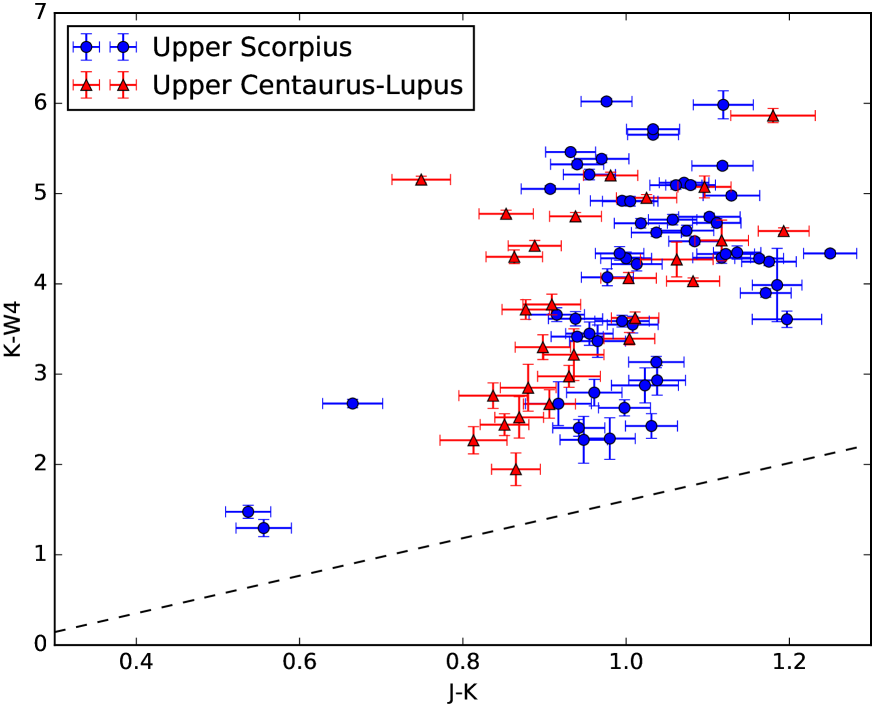
Figure 1: Colour-colour plot of $K-W4$ against the $J-K$ colours. The dashed lines show the expected $K-W4$ colour based on the photospheric sequence.

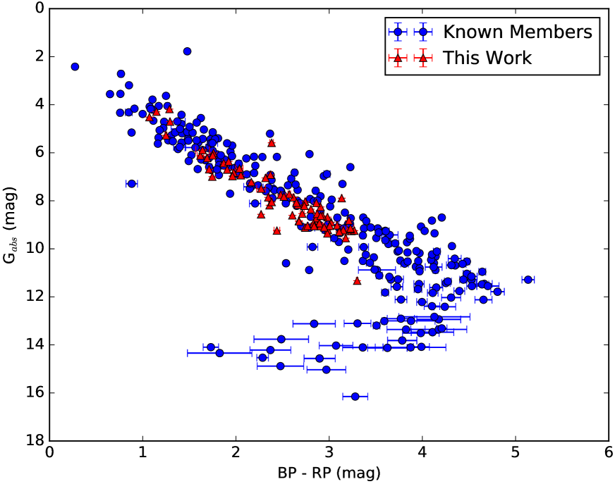
Figure 2: Colour-magnitude of our targets (red) against previously known members of the Scorpio-Centaurus star forming region (blue). Magnitudes are taken from Gaia (G Mag) and the color is determined from the Gaia Blue band (BP) and Red band (RP) photometry (Gaia Collaboration et al. 2016; Gaia Collaboration et al. 2018). Known members are shown in blue and are taken from Pecaut & Mamajek (2016); Luhman & Mamajek (2012); Aarnio et al. (2008); Preibisch et al. (1998); Chen et al. (2011); Martín et al. (2004); Meyer et al. (1993); Köhler et al. (2000); Martín et al. (1998); Bouvier & Appenzeller (1992); Kraus & Hillenbrand (2009); Lodieu et al. (2006); Erickson et al. (2011); Slesnick et al. (2006); Wilking et al. (2005); Oliveira et al. (2010); Cieza et al. (2010); Luhman & Rieke (1999); Doppmann et al. (2003); Natta et al. (2002); Elias (1978); Walter et al. (1994); Ardila et al. (2000); Lodieu et al. (2011); Martín et al. (1998); Lodieu et al. (2008); Preibisch et al. (2002); Herbig & Bell (1988); Vieira et al. (2003). The targets observed in our work is shown in red.

IR excess is searched for in our target members of Upper Scorpius and Upper Centaurus-Lupus. These targets were visually inspected on the IRSA WISE image service to check for obscuration by a cloud or contamination by a nearby IR bright object. Some objects were discarded and the final survey used 55 US targets and 28 of UCL targets were found to exhibit IR excesses. The targets are plotted in a colour-magnitude diagram against other known Scorpio-Centaurus members in Figure 2. The color-magnitude diagram is produced using magnitudes from Gaia (Gaia Collaboration et al. 2016; Gaia Collaboration et al. 2018) and summarised in Table 5. This shows that our targets are likely to be members of the Sco-Cen star forming region. The positions of our targets are also plotted in Figure 3 and are summarised in Table 6. Our targets have large angular separations from the Lupus star-forming clouds. Therefore we believe it is unlikely that we have interlopers from this significantly younger association in our sample. After our disc-bearing targets had been identified they were observed to search for radial velocity (RV) variation which may indicate the presences of a companion.

2.3 Spectroscopic observations to obtain radial velocities

2.3.1 WiFeS observations

To obtain spectroscopic data to determine the radial velocities of our targets, we used the Wide Field Spectrograph (WiFeS) (Dopita et al., 2007). WiFeS is an integral field spectrograph on the Australian National University 2.3m Telescope at Siding Spring Observatory. We use this instrument to search for radial velocity variation over time for our targets. The instrument consists of a blue camera with spectral range $329-558\,\mathrm{nm}$ and red camera with spectral range $529-912\,\mathrm{nm}$.

Data for our targets was collected from June of 2013 to July of 2017. Our observations include Ne-Ar arc exposures every 15-30 minutes to characterise the wavelength scale variation of the instrument over the night due to temperature fluctuations. The WiFeS $R\sim 7000$ grating is used to perform radial velocity measurements. We observe radial velocity standards with well characterised velocities of various spectral types. Radial velocity standards are selected from Nidever et al. (2002) and Soubiran et al. (2013) (detailed in Table 1). Observations of radial velocity standards are bracketed by arc lamp exposures and further correction to the calibrations is applied using oxygen B-band atmospheric absorption lines (static with respect to the observer). The calibration using the oxygen B-band lines is dependent on stellar type and signal-to-noise of each individual target. Data are reduced using the PyWiFeS pipeline (Childress et al., 2013).

2.3.2 Radial velocity precision based on RV standards

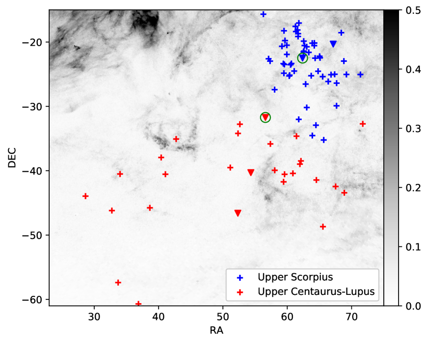
Figure 3: A map of the candidate disc-bearing stars in Upper Scorpius (US, the blue markers) and Upper Centaurus-Lupus (UCL, the red markers) that we consider in this study. The background image is an extinction map compiled by Schlafly et al. (2014). The triangle markers indicate objects that we believe to be binary star systems because they have Bayes factor (described by Equation 7 in Section 3.2) greater than 300. The circled triangles highlight two double-lined spectroscopic binaries found in this work (described in 2.3.3)

RV Standard	$v_{r}$ (km/s)	Sp. Typ.	Approx. Mass (M⊙)
HD35974	76.683	G1Va	1.40
HD144585	-14.067	G2Vb	1.38
HD145809	21.146	G2Vc	1.38
HD141885	-16.160	G3Va	1.37
HD1461	-10.166	G3Vb	1.37
HD189625	-28.218	G5Vd	1.35
HD19034	-20.344	G5Ve	1.35
HD198802	-3.171	G5Ve	1.35
HD153458	0.641	G5Ve	1.35
HD37213	12.464	G5Va	1.35
HD128428	-42.074	G6IVe	1.34
HD196761	-41.987	G7.5IV-Vb	1.32
HD283	-43.102	G9.5Vc	1.29
HD156826	-32.634	K0Ve	1.26
HD114783	-12.012	K1Ve	1.23
HD32147	21.552	K3+Vc	1.15
HD2025	3.241	K3Vc	1.15
HD130992	-57.160	K3.5Vc	1.12
HD170493	-54.752	K4Ve	1.10
HD120467	-37.806	K6Vab	0.90
GJ173	-6.768	M1Vg	0.55
GJ433	17.973	M1.5f	0.50
GJ2066	62.205	M2Vh	0.45
GJ382	7.932	M2Vi	0.45
GJ357	-34.581	M2.5Vc	0.40
GJ273	18.216	M3.5Vi	0.20
GJ729	-10.499	M3.5Vej	0.20

Table 1: Radial velocity standards used as templates to obtain radial velocities of our observed targets. Standards are selected from the Nidever et al. (2002) and Soubiran et al. (2013) catalogues. ^aHouk (1982), ^bKeenan & McNeil (1989), ^cGray et al. (2006), ^dHouk & Smith-Moore (1988), ^eHouk & Swift (1999), ^fHenry et al. (2002), ^gStephenson (1986), ^hAlonso-Floriano et al. (2015), ⁱKirkpatrick et al. (1991), ^jDavison et al. (2015). The approximate masses are derived from the Baraffe et al. (2015) pre-main sequence evolution models based on spectral type at age log${}_{10}($t${}_{age})\sim 7.1$.

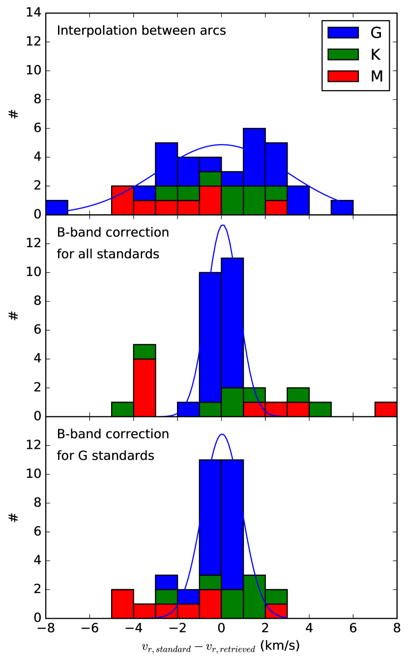
Figure 4: Precision in retrieving the radial velocity of RV standards. $\Delta v_{r}$ is the difference between the radial velocity of the RV standard and the retrieved radial velocity using our pipeline. The blue, green, red and magenta histograms show the precision of the G-, K- and M-type RV standards respectively. Top: precision when only using the wavelength solutions produced by linear interpolation between arcs (as produced by PyWiFeS). Middle: precision when the oxygen B-band absorption lines are also used to further calibrate the wavelength scale. Bottom: precision when the oxygen B-band absorption lines are only used for further calibration on the G-type RV standards.

Radial velocity standards of spectral types varying from G1 through to M3.5 (see Table 1) were observed with WiFeS to create spectral templates. These templates are cross-correlated with our targets to determine their radial velocity using the post-processing tools developed for WiFeS. Obtained radial velocities are correct to be in heliocentric velocity frame.

The radial velocity standards were observed using the settings described in Section 2.3. After the observations of the RV standards were reduced, their wavelength scale was shifted to the rest frame. This product was used as the template from which the radial velocity of the targets is obtained.

Tests of retrieving the radial velocity of the RV standards after creating templates of the observed spectra were run. This was done by cross-correlating the reduced spectra of the observed RV standards with created templates, ensuring that the standard was not cross-correlated with itself. We found that the retrieved radial velocities had a relatively large spread from the actual radial velocity of the RV standards with standard deviation of $3.0\,\mathrm{km/s}$ (top panel of Figure 4). We believe this is because the WiFeS instrument may vary on a shorter time-scale than 15-30 minutes. The wavelength scale solution is the linear interpolation between that derived from nearby arcs, as done by the PyWiFeS pipeline, was therefore not accurate enough for the purposes of our work.

In order to improve our radial velocity precision we use the oxygen B-band atmospheric absorption lines and sky emission. Using the oxygen B-band absorption lines we could determine the offset from the wavelength solution derived from PyWiFeS. The precision of retrieving the radial velocity of the RV standards with the added correction from the B-band is shown in the middle panel of Figure 4. We see that the precision is increased significantly for the G standards, but is decreased for K and M standards. This is not surprising as K and M type stars have emission in the wavelength region of the oxygen B-band absorption, which makes it difficult to determine a velocity. The overall standard deviation of the precision when applying the correction from the B-band absorption reduced to $0.7\,\mathrm{km/s}$.

In addition to using oxygen B-Band absorption lines to improve radial velocity precision, emission from skylines was also tested. This proved to not be useful because the RV standards are very bright, therefore not enough signal-to-noise is obtained to confidently retrieve a radial velocity.

RV standard spectral type	$\sigma$ (km/s)
G	0.7
K	1.4
M	2.3

Table 2: Precision of retrieving RV standard radial velocity per spectral type

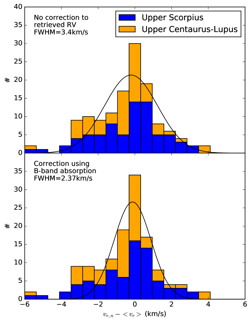
Figure 5: Radial velocity variation distributions for observed objects calculated as the difference between the radial velocity of the objects last, nth, epoch ($v_{r,n}$) and the objects mean radial velocity over all epochs ($<v_{r}>$). Top: shows the distribution without correction from the absorption lines. The full-width-half-maximum of the fitted gaussian is $3.40$ km/s. Bottom: shows the radial velocity variation with the added correction from the absorption lines. The full-width-half-maximum of the fitted gaussian is $2.37$ km/s

Based on the results of this investigation, we decided to only apply calibrations to the G type RV standards by correcting the radial velocity from the shift measured in the B-band absorption. The resulting precision is shown in the bottom panel of Figure 4. The overall standard deviation of the precision using this combination of velocity calibrations is $0.9\,\mathrm{km/s}$, which is a slight increase from applying the B-band absorption correction to all RV standards, but the standard deviation per spectral type is improved. The standard deviation per spectral type is summarised in Table 2.

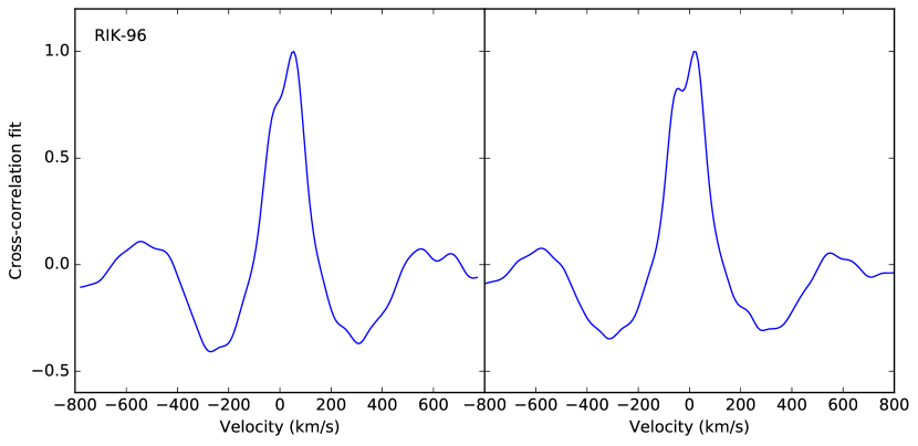
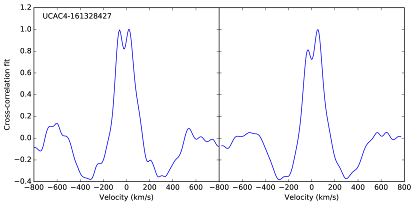
Figure 6: Cross-correlations of the two SB2s found. The y-axis has arbitrary units of a measure of fit. The top two panels show cross-correlations for RIK-96 and the bottom two show cross-correlations for UCAC4-161328427 at two different epochs.

2.3.3 Obtaining radial velocity of targets

To obtain the radial velocity of our targets, observations are cross-correlated with all the RV standards in an initial step. In order to cross-correlate the target spectra with the template spectra the H$\alpha$ region had to be masked out as most of our targets have strong H$\alpha$ emission (discussed further in Section 2.4). Each object is then set a preferred RV standard template to make sure all epochs are cross-correlated with the same template. In the initial step an object will mostly cross-correlate the best with the same template over all epochs or with templates of similar spectral type. An object’s preferred template is the template that it correlates the best with over most of the epochs.

After a preferred template is selected, radial velocities are determined again, with all epochs cross-correlating with the same template. Correction using the oxygen B-band absorption is also applied to the obtained radial velocities. The added correction from the absorption lines does show an improvement on the radial velocities precision. When plotting a histogram of radial velocity variation, we expect a large fraction of objects to possess a variation near $0\,\mathrm{km/s}$, which are the objects that are single stars. From our observations, the radial velocity variation is taken to be the difference between the objects last, nth, epoch ($v_{r,n}$) and the objects mean radial velocity over all epochs ($<v_{r}>$), i.e.

$$\Delta v_{r}=v_{r,n}-<v_{r}>.$$ (1)

A histogram of radial velocity variation for our targets is shown in Figure 5. The full-width-half-maximum (FWHM) of this histogram can be taken as a precision of the radial velocity measurements. We see that the reduces from $3.40\,\mathrm{km/s}$ to $2.37\,\mathrm{km/s}$ when corrections using the oxygen B-band absorption is applied (Figure 5).

We identify two double-lined spectroscopic binaries (SB2s). RIK-96 is found in Upper Scorpius and UCAC4-161328427 in Upper Centaurus-Lupus. Cross-correlations at two epochs for each of the SB2s are shown in Figure 6. Both objects show very strong IR excesses, which likely indicate the presences of a large circumbinary disc. We carried out two dimensional cross-correlations with templates for these objects to estimate the spectral type and flux ratio of the components. We find for RIK-96 the primary and secondary to be of spectral type M1.5 and M2.5 respectively, with a flux ratio of $\sim 0.71$. We find for UCAC4-161328427 that both components fit best to M2.5 templates, with a flux ratio of $\sim 0.98$. Information about these two objects is summarised in Table 3.

2.4 H$\alpha$ as a youth indicator

As mentioned in 2.3.3 the observed targets showed H$\alpha$ emission that hindered cross-correlations with template spectra. The H$\alpha$ emission is believed to be caused by accretion of disc material onto the stars. In Figure 7, we display the measured H$\alpha$ equivalent widths for the targets. The majority of the targets members show some level, of H$\alpha$ emission, with a clear sequence of increasing emission with spectral type. Rizzuto et al. (2015) uses the combination of lithium and H$\alpha$ emission as indicator of youth for the identified RIK objects. Of our 55 US and 28 UCL targets, $\sim 82\%$ and $\sim 70\%$ show H$\alpha$ emission with ($\mathrm{EW(H\alpha)}<-1\AA$). Of the members that do not show or show weak H$\alpha$ emission, most are earlier than M0 spectral type based on the template spectra used for cross-correlation.

3 Results and Statistical Analysis

Using a hard cut of $5\sigma$ significance on the radial velocity variation for the fraction of binaries in Upper Scorpius and Upper Centaurus-Lupus we get 15$\%$ and 10$\%$ respectively. The fractions produced from this criterion only find the closest binaries, which produce the greatest radial velocity variation. In order to better characterise the binaries that we do not detect we must use Bayesian statistics to explore the parameter space.

3.1 Simulating Systems

The radial velocity ($v_{r}$) of the primary star in a binary system can be described by:

$$v_{r}=K[\cos(\omega+\Omega)+e\cos\omega]+v_{sys},$$ (2)

where $K$ is a constant described below, $\omega$ is the longitude of periastron, $\Omega$ is the position angle of the line of nodes, $e$ is the eccentricity of the system and $v_{sys}$ is the system velocity. $K$ is described by:

$$K\equiv\frac{2\pi}{P}\frac{a_{1}\sin i}{(1-e^{2})^{1/2}},$$ (3)

where $P$ is the period of the system, $a_{1}$ is the semi-major axis of the primary star from the barycentre of the system and $i$ is the inclination of the binary. $a_{1}$ for a system can be calculated for a binary when the period and component masses are known. From the primary mass and mass ratio, the semi-major axis can be determined from Kepler’s third law:

$$a=(M_{1}(1+q)P^{2})^{1/3},$$ (4)

where $a$ is the semi-major axis of the system, $M_{1}$ is the mass of the primary star and $q$ is the mass ratio between the secondary and primary components, i.e. $q=M_{2}/M_{1}$. From the binary mass function the semi-major axis of the primary component can be determined from:

$$a_{1}=a\frac{q}{1+q}.$$ (5)

In our Bayesian analysis, we simulate radial velocity curves using $\omega$, $\Omega$, $i$, $e$, $P$, $T_{0}$, $v_{sys}$, $M_{p}$ and $q$ sampled from appropriate parameter spaces described in the next section.

3.2 Bayesian Statistics

	RIK-96	UCAC4-161328427
RA	16 09 31.66	15 46 25.81
DEC	-22 29 22.4	-31 43 19.3
$J-K$	0.995	0.863
$K-W4$	4.922	4.305
SpT of Primary	M1.5	M2.5
SpT of Secondary	M2.5	M2.5
Flux ratio	0.71	0.98
Epoch 1
$v_{\mathrm{r,left}}$(km/s)	$-57.5\pm 0.3$	$-63.4\pm 0.9$
$v_{\mathrm{r,right}}$(km/s)	$26.5\pm 0.2$	$24.3\pm 1.0$
$v_{\mathrm{heliocentre}}$(km/s)	16.9	23.1
Epoch 2
$v_{\mathrm{r,left}}$(km/s)	$-31.3\pm 1.0$	$-39.5\pm 0.7$
$v_{\mathrm{r,right}}$(km/s)	$57.9\pm 0.7$	$56.7\pm 0.7$
$v_{\mathrm{heliocentre}}$(km/s)	-10.2	-5.9

Table 3: Summary of the SB2s found. The assigned spectral type of the components is based on the best fitting template.

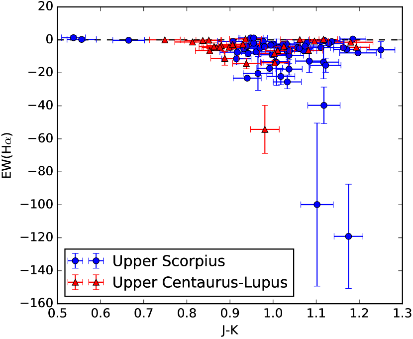
Figure 7: Mean H$\alpha$ equivalent width for our targets measured over all epochs. The error bars is the standard deviation of the measured equivalent width over all epochs.

Symbol	Parameter	Lower Bound	Upper Bound	Distribution
$\omega$	Longitude of periastron	$0^{\circ}$	$360^{\circ}$	Uniform
$\Omega$	pos. ang. of the line of nodes	$0^{\circ}$	$360^{\circ}$	Uniform
$i$	Inclination	$0^{\circ}$	$90^{\circ}$	Sinusoidal
$e$	Eccentricity	$0$	$0.95$	Uniform
$P$	Period	$1\,\mathrm{day}$	$7300\,\mathrm{days}$	Log normal
$T_{0}$	Time of Periastron Passage	$0\,\mathrm{days}$	$P$	Uniform
$v_{sys}$	system velocity	$<v_{r}>-4\,\mathrm{km/s}$	$<v_{r}>+4\,\mathrm{km/s}$	Gaussian
$M_{p}$	Mass of Primary	$M_{template}-0.1M_{template}$	$M_{template}+0.1M_{template}$	Uniform
$q$	mass ratio	$0.05$	$1.0$	Uniform

Table 4: Priors for Bayesian analysis.

Some of these priors are independent from the physical characteristics of the system, such as $\omega$, $\Omega$ and $i$, therefore the parameter space from which these quantities are sampled is the same for all objects. The parameter spaces that the period, time of periastron passage and eccentricity are sampled from also remain the same for all objects because these quantities directly influence the shape of the radial velocity curve. The parameter space sampled for the system velocity is dependent on the observed radial velocities, therefore this space is redefined for each object, as described in Section 3.3.

Initially all random orbits are given an amplitude of $1\,\mathrm{km/s}$, but this is scaled when considering the possible mass of the primary star and the mass ratios. For each object $\omega$, $\Omega$, $i$, $P$, $T_{0}$, $e$ and $v_{sys}$ are sampled $10^{5}$ times to produce radial velocity curves with normalised amplitudes. Then for each of these orbits $M_{p}$ and $q$ are sampled $10^{2}$ times to scale these normalised radial velocity curves. The parameter space that the primary mass is sampled is dependent on the template that the object cross-correlates with. The parameter space that the mass ratio is sampled from is the same for all objects.

Once a radial velocity curve is simulated, a likelihood of fit is calculated for each simulated orbit given by:

$$L\propto e^{-\frac{(v_{r,obs}-v_{r,sim})^{2}}{2\sigma_{obs}^{2}}},$$ (6)

where $v_{r,obs}$ is the observed radial velocity, $v_{r,sim}$ is the simulated radial velocity, and $\sigma_{obs}$ is the error on the measured radial velocity. The error of the measured radial velocity is the error derived from the cross-correlation, the error from the precision of the template used and a standard astrophysical error added in quadrature. The standard astrophysical error accounts for variations caused by stellar activity or rotation and is set to $1\,\mathrm{km/s}$. Our results are shown not to vary significantly for an astrophysical error over the range of $0.5-2.0\,\mathrm{km/s}$. The error on the precision of the RV standard template is taken from Table 2.

Likelihoods are also calculated for fitting a single star i.e. a constant radial velocity. The velocity for a single star fit is taken to be the system velocity ($v_{sys}$) that is sampled for the simulated binary star orbit.

After all the radial velocity curves for the simulated orbits have likelihoods calculated, we calculate the mean likelihood of the data given our two models, $P(D|S)$ and $P(D|B)$. From these, the Bayes factor is calculated, which is given by:

$$\Upsilon=\frac{P(D|B)}{P(D|S)},$$ (7)

From this we see that the Bayes factor is simply the ratio of the mean likelihoods of being a binary star to a being a single star. A binary model is preferred if $\Upsilon\gg 1$ and a single star model is preferred if $\Upsilon\ll 1$. Where $\Upsilon\approx 1$, either model is equally probable. We take objects with Bayes factors $>300$ to be binary stars as this is near the $3\sigma$ confidence level assuming a Gaussian probability distribution. Using this threshold we find five objects to be binary stars, including the two double-lined binaries shown in Figure 6 and listed in Table 3. The Bayes factors for every target can be found in Table 6

Once the Bayes factor is calculated for each target we calculate the binary fraction. The likelihood of being a binary or multiple star system, $P(B)$, is complimentary to the likelihood of being a single star, $P(S)$. Therefore, if we take the likelihood of being a binary to be $\gamma$, then $P(B)=\gamma$ and $P(S)=1-\gamma$. This is described statistically like a Bernoulli trial. The Jeffreys’ prior to this case states that the probability of $\gamma$ can be described by:

$$P(\gamma)\propto\frac{1}{\gamma(1-\gamma)}.$$ (8)

We are trying to find what the probability density function of $\gamma$ is for Upper Scorpius and Upper Centaurus-Lupus. Following Bayes’ Theorem, the probability of $\gamma$ given our data is:

$$P(\gamma|D)=\frac{P(\gamma)}{P(D)}P(D|\gamma).$$ (9)

We can expand out the probability of the data given $\gamma$, $P(D|\gamma)$, into constituents of the probability of being a single or binary star given $\gamma$, $P(S|\gamma)$ and $P(B|\gamma)$ respectively, giving:

$$P(\gamma|D)=\frac{P(\gamma)}{P(D)}[P(D|B)P(B|\gamma)+P(D|S)P(S|\gamma)].$$ (10)

As $\gamma$ is defined as the multiplicity, $P(B|\gamma)\equiv\gamma$ and $P(S|\gamma)\equiv 1-\gamma$ as described previously. This gives us:

$$P(\gamma|D)=\frac{P(\gamma)}{P(D)}[P(D|B)\gamma+P(D|S)(1-\gamma)].$$ (11)

We can express Equation 11 in terms of our Bayes’ factor, which we calculate from our observations. The probably of $\gamma$ given the data is now:

$$P(\gamma|D)=\frac{P(\gamma)}{P(D)}P(D|S)[\Upsilon\gamma+(1-\gamma)].$$ (12)

Or to simplify:

$$P(\gamma|D)\propto P(\gamma)[\Upsilon\gamma+(1-\gamma)].$$ (13)

Where $P(\gamma)$ is our prior on the probability distribution of the binary fraction. Our initial guess is that the probability distributions of $\gamma$ is uniform, meaning that every possible binary fraction is equally likely. This prior is updated with the Bayes’ factor of each object. For the first object, the probability of $\gamma$ given the data is:

$$P(\gamma|D)_{1}\propto P(\gamma)_{0}[\Upsilon_{1}\gamma+(1-\gamma)].$$ (14)

Where $P(\gamma)_{0}$ is our initial guess of a uniform distribution. This is saying that we believe this object has an equal probability of being a single or binary star and it is updated with the Bayes factor of the first object. This updated prior becomes the prior for the next object. Expanding this to $nobjects$ we get:

$$P(\gamma|D)\propto P(\gamma){\displaystyle\prod_{i=1}^{n}}[\Upsilon_{i}\gamma+(1-\gamma)].$$ (15)

3.3 Bayesian priors

The priors for our Bayesian analysis are summarised in Table 4. $\omega,\Omega$ and $i$ are all independent of physical characteristics of the binary star system. These quantities account for projection effects on the observed radial velocity and may have any orientation, i.e. are isotropic. We sample inclination $i$ from a distribution proportional to sin($i$), and sample the position angle of the line of nodes, $\Omega$, and longitude of periastron, $\omega$, from 0^∘ to 360^∘ in order to uniformly sample the three-dimensional orientation of orbits.

The eccentricity of an object may be $e=0$ for a circular orbit, up to $e=1$ for a parabolic orbit. We sample the eccentricity from a uniform distribution as Raghavan et al. (2010) find that eccentricity follows a mostly uniform distribution up to $e=0.6$. The lower bound for our eccentricity parameter space is $e=0$ and the upper bound is $e=0.95$.

The largest baseline our observations have is $\sim$4$\,\mathrm{yrs}$. With this baseline we take the largest binary orbital period that we should be able to detect to be $7300\,\mathrm{days}$ or $\sim$20$\,\mathrm{yrs}$. We take the shortest possible period to be $1\,\mathrm{day}$. The periods are sampled from a log-normal distribution with a mean of $\mu_{P}=5.03$ and standard deviation $\sigma_{P}=2.28$ as found by Raghavan et al. (2010). The time of periastron passage, $T_{0}$, is essentially the phase of the radial velocity curve and is dependent on the period. All values of $T_{0}$ are equally likely, so this value is sampled from a uniform distribution from $0$ days to $P$ in days.

We aim to marginalise our probability distributions over all possible values of the centre of mass velocity, because the dispersion of velocities within our association is larger than our typical velocity precision. For computational speed, we only sample values of $v_{sys}$ from a normal distribution centred on the mean radial velocity over all epochs of an object and with a standard deviation of 4$\,\mathrm{km/s}$ (larger than our typical uncertainties). Sampling from a wider distribution would lower both the single and binary star probabilities roughly equally and would not noticeably affect our results.

It is reasonable to assume that the best fitting spectral template corresponds to the brighter component of a binary star system. From this assumption we sample the mass of the primary, $M_{p}$, based on the template that was used to derive radial velocities. The typical mass of a main sequence star for the spectral type of the template is used as a guide for $M_{p}$. The typical spectral type mass for each template can be found in Table 1. $M_{p}$ is sampled from a uniform distribution with lower and upper bounds being $\pm 10\%$ of the typical mass of the template. The mass ratio, $q$, is sampled from a uniform distribution as this is what observations have shown (Raghavan et al., 2010). For our work we set a minimum mass ratio of $q=0.05$.

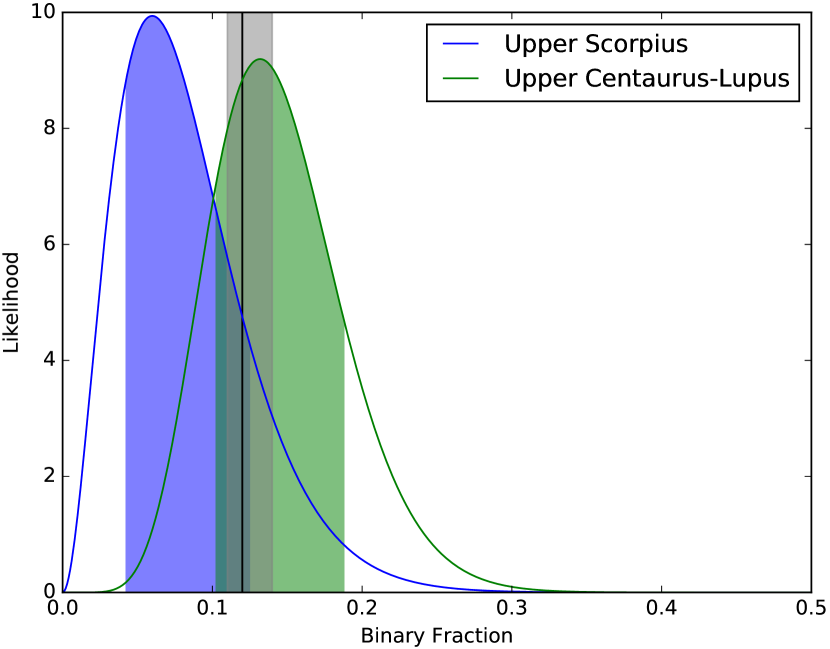
Figure 8: The normalised probability distribution of multiplicity for our disc-bearing stars in Upper Scorpius and Upper Centaurus-Lupus. The y-axis is in arbitrary units. The vertical line and shaded region highlights our expected binary fraction of $\sim 0.12^{0.02}_{0.01}$ based on the multiplicity of field stars irrespective of whether they have discs or not. The mean likelihood fractions of US and UCL are $0.06^{0.07}_{0.02}$ and $0.13^{0.06}_{0.03}$ respectively.

When carrying out this calculation for our objects in Upper Scorpius and Upper Centaurus-Lupus, we find that the maximum likelihood binary fractions to be $0.06^{0.07}_{0.02}$ and $0.13^{0.06}_{0.03}$ respectively. The mean likelihoods for Upper Scorpius and Upper Centaurus-Lupus are $0.08$ and $0.14$ respectively. The normalised posterior density functions are shown in Figure 8. The error bars are the 16th and 84th percentile, and are highlighted in Figure 8.

4 Discussion

4.1 Binary fraction and implication on disc lifetime

From our work we find that approximately one fifth of disc-bearing stars of spectral types F and later in Upper Scorpius (US) and Upper Centaurus-Lupus (UCL) are in binary star systems with periods less than 20 years.

Raghavan et al. (2010) find the multiplicity of $\sim 1.25-1.02$ M_⊙ stars to be $54\%\pm 4\%$ and $\sim 1.02-0.78$ M_⊙ stars to be $41\%\pm 3\%$. Shan et al. (2017) find a raw multiplicity of $\sim 0.9-0.07$ M_⊙ dwarfs to be $35\%\pm 3\%$. From these multiplicities found in the literature and the masses of our targets (based on the template fitted to the target, see 2.3.3) we calculate an expectation value for the binary fraction based on the field population. Based on the templates fit to our targets we have 6 US and 4 UCL objects $\geq 1.02$ M_⊙, 7 US and 8 UCL objects between $1.02-0.78$ M_⊙ and 42 US and 16 UCL objects below $\sim 0.78$ M_⊙. Under the assumption that binary stars of all spectral types follow the same log-normal orbital period distribution as described by Raghavan et al. (2010), we are able to detect up to $31\%$ of all binary systems (because $31\%$ of the log-normal period distribution is below a period of 20 years). Based on the binary fractions and the fraction of detectable binary star systems, we expect $\sim$1 US and UCL target $\geq 1.02$ M_⊙, $\sim$1 US and UCL between $1.02-0.78$ M_⊙ targets, and $5\pm 0.5$ of our US and $\sim 2$ of our UCL objects below $0.78$ M_⊙ to be binaries. This gives a total expectation value of $7\pm 0.5$ out of the 55 US targets and $3.5\pm 0.5$ out of the 28 UCL targets to be binaries, or an expected fraction of $\sim 0.12^{0.02}_{0.01}$ for both regions if they followed the same binary statistics as the field stars in Raghavan et al. (2010). This is consistent with our fractions obtained from the Bayesian analysis.

Our results show that the binary fraction of our targets showing IR excess is tentatively consistent with the binary fraction of the general stellar population implying that the overall the lifetime of discs in binary star systems is comparable to single stars. Our work does not discriminate between circumbinary discs and circumstellar discs around individual components in a binary star system. There may be variations in disc lifetime depending on the configuration of the system. Damjanov et al. (2007) and Harris et al. (2012) find that binaries of separation $\mathrel{\hbox{\hbox to0.0pt{\hbox{\lower 3.0pt\hbox{${\sim}$}}\hss}\hbox{\raise 2.0pt\hbox{$<$}}}}$30$\,\mathrm{AU}$ have significantly smaller IR excess compared to other binary stars with discs, which may indicate that a close companion leads to faster disc dispersal. This is in contrast to many massive, bright circumbinary discs (Harris et al. 2012; Cox et al. 2017) which could indicate the opposite. A binary star has more angular momentum compared to a single star of the same total mass, so one would expect a binary star system to host a larger disc than it’s single star counterpart. The primary of a binary star system would also accrete less rapidly than a single star of the combined mass of binary components, which would lead to a slower photo-evaporation process, leading towards a longer lifetime. Daemgen et al. (2016) find that the fraction of accretion discs around binary stars is a factor of $\sim 2$ lower than accretion discs around single stars in the Chamaeleon I region. This may be because circumbinary discs have the gas evacuated from the inner region by a close companion, leading to lower accretion rates. This could contribute to circumbinary discs having a longer typical lifetime and explain some very old circumbinary discs. These various factors could average out over the long term leading to similar disc lifetimes in single star and binary star systems.

4.2 Caveats

In this work we use Bayesian statistics to account for the limited set of observations on this study. As such, we must discuss some of the caveats associated with our conclusions.

Only the two double-lined spectroscopic binaries presented in Figure 6 can be conclusively identified as binaries. For the remainder of our objects, binarity is determined from a combination of a detected radial velocity variation and Monte-Carlo simulations. This is because no single object has had a sufficient number of radial velocity observations to resolve a full orbit, with only 2-7 epochs, with a median of 4 epochs per target.

Additionally, given we have only two conclusively identified binary systems, our work gives a raw binary fraction which is consistent with no multiplicity in the sample. Therefore, the suggestion that discs in binary star systems are heavily hindered leading to the quick dispersal of discs in binaries of periods up to 20 years is also valid based on our data.

The $22\mu$m emission detected by the WISE W4 band traces disc emission out to a few AU, whereas millimetre surveys from Harris et al. (2012) and Cox et al. (2017) trace regions that are further out. This makes comparison with previous work difficult as the infrared emission measured in this work probes a different region of the IR spectrum. Our work looks at the survival time of the inner region of discs, which may be truncated in circumbinary discs. But these same circumbinary discs would, nevertheless, exhibit millimetre emission.

Our target sample is also biased against massive stars (i.e. greater than $\sim 1.4$ M_⊙). This is mainly due to a lack of absorption lines needed for precise cross-correlation with a template. This may be problematic in the context of determining multiplicity as many surveys (Raghavan et al., 2010) show that multiplicity increases with primary star mass. But the overall multiplicity of disc-bearing objects would be more sensitive to the initial mass function used and the populations of lower-mass stars. Therefore we believe that excluding massive stars is unlikely to change our results significantly.

5 Summary and Conclusion

We determine the multiplicity of disc-bearing stars in the $\sim$11$\,\mathrm{Myr}$ Upper Scorpius (US) and $\sim$17$\,\mathrm{Myr}$ Upper Centaurus-Lupus (UCL) for periods up to 20 years. Our sample consists of 55 US members and 38 UCL members that are shown to have an IR excess, indicating the presence of a disc. Targets are observed with the Wide Field Spectrograph (WiFeS) on the Australian National University 2.3m telescope to search for radial velocity variation.

Using Bayesian statistics we determine the binary fraction of our disc-bearing stars in Upper Scorpius and Upper Centaurus-Lupus to be $0.06^{0.07}_{0.02}$ and $0.13^{0.06}_{0.03}$ respectively. When compared to the expected binary fraction of $\sim 0.12^{0.02}_{0.01}$ based on our observational limits and the multiplicity of field stars, these results are consistent with disc lifetime around binary stars being similar to single stars. This implies that planet formation is equally likely around binary stars as around single stars.

Appendix A Targets

Listed in Table 5 is the $J$ and $K$ magnitudes for our targets taken from the 2MASS survey (Skrutskie et al., 2006). The W4 magnitude is take from the AllWISE source catalogue (Wright et al., 2010). We use Gaia (Gaia Collaboration et al. 2016; Gaia Collaboration et al. 2018) to obtain Gaia magnitudes (G Mag) as well as Blue band (BP) and Red band (RP) photometry.

Listed in Table 6 is the full list of targets observed in this survey.

The probability of membership, P(M), is calculated based on the calculations of Rizzuto et al. (2011) and Rizzuto et al. (2015) which uses kinematic and spatial information to assign a probability (see Section 2.1).

$\Delta v_{r}$ is the observed radial velocity variation over all epochs. The radial velocity variation is taken to be the difference between the epoch with the highest radial velocity and the epoch with the lowest radial velocity, (see Equation 1).

$\Upsilon$ is the Bayes factor calculated as described in Section 3.2. A binary star model is preferred if $\Upsilon\gg 1$ and a single star model is preferred if $\Upsilon\ll 1$. Where $\Upsilon\approx 1$, either model is equally probable. We take objects with Bayes factors $>300$ to be binary stars as this is near the $3\sigma$ confidence level assuming a Gaussian probability distribution.

Table 5: Magnitudes of our targets. J and K magnitudes are taken from the 2MASS survey. W4 magnitude is taken from the AllWISE source catalogue. The G, BP and RP magnitudes are taken from the Gaia survey.

Object	RA	DEC	$J$	$K$	$W4$	$G$	$BP$	$RP$
UCAC4-827387234	13 54 35.61	-43 56 48.1	11.638	10.708	7.732	14.46715	15.951675	13.276466
UCAC4-467124593	14 10 59.69	-46 11 33.8	11.196	10.343	5.567	14.351444	16.073818	13.087802
UCAC4-947158099	14 14 52.40	-57 22 54.0	13.262	12.2	7.93	15.941499	17.134708	14.865117
UCAC4-382098779	14 16 03.10	-40 30 34.2	11.014	10.149	8.202	13.938769	15.460843	12.718367
UCAC4-945204860	14 27 30.11	-60 42 18.0	12.588	11.492	6.418
UCAC4-442012351	14 34 36.62	-45 45 59.9	11.725	10.845	7.995	14.812784	16.228548	13.460551
UCAC4-371257082	14 41 37.66	-37 56 34.4	11.746	10.837	7.065	14.544952	15.975403	13.370145
UCAC4-371337294	14 44 15.62	-40 32 27.3	11.654	10.766	6.344
UCAC4-21594717	14 50 55.74	-35 04 22.9	10.892	10.055	7.293	12.948328	13.802399	12.056115
UCAC4-365499547	15 24 35.62	-39 30 43.3	11.56	10.691	8.169	14.581901	16.145092	13.340626
UCAC4-445278523	15 29 17.48	-46 36 28.7	12.51	11.574	8.358	13.758428	14.996365	12.6358185
UCAC4-23251943	15 29 23.88	-34 11 54.5	11.535	10.637	7.338
UCAC4-23288203	15 30 33.57	-32 46 19.1	11.08	10.174	7.504
UCAC4-447414452	15 37 22.69	-40 17 59.6	8.796	7.771	2.818	10.21763	10.68769	9.616082
UCAC4-333669217	15 45 09.50	-15 40 29.0	11.808	10.795	6.576	15.126357	17.03052	13.792687
UCAC4-161328427	15 46 25.81	-31 43 19.3	11.468	10.605	6.305	14.510724	16.173733	13.265781
UCAC4-30196323	15 48 24.44	-22 35 49.7	11.868	10.732	6.385	15.303416	17.155664	13.978409
UCAC4-30231541	15 49 19.76	-22 57 29.7	10.534	9.536	6.909	13.884282	15.718709	12.584246
UCAC4-1297314504	15 49 30.74	-35 49 51.4	10.96	10.022	5.274	13.875682	15.305055	12.686407
UCAC4-408863727	15 52 08.84	-27 23 45.8	11.996	11.019	6.946	15.29399	16.951279	14.044705
UCAC4-1019544336	15 52 13.44	-39 56 08.2	11.705	10.828	7.112	14.595463	16.07941	13.4024315
RIK-23	15 56 42.45	-20 39 34.2	11.313	10.28	4.628	14.495734	16.086412	13.223093
RIK-30	15 57 34.31	-23 21 12.3	9.932	8.992	5.576	12.7145195	13.970277	11.600752
UCAC4-519496506	15 57 43.61	-41 43 37.8	9.825	8.743	4.713	12.037338	12.895082	11.136776
UCAC4-426579903	15 57 54.45	-24 50 42.4	9.51	8.578	3.118	11.776407	12.5178175	10.898948
UCAC4-404438620	15 57 58.92	-18 14 59.6	9.991	8.92	3.8	12.300475	13.221161	11.352783
RIK-34	15 58 12.70	-23 28 36.4	8.574	8.018	6.722	10.07295	10.586112	9.43927
UCAC4-519508031	15 58 20.40	-40 33 05.8	10.563	9.582	4.381	13.720713	14.981765	12.501845
RIK-38	15 58 36.20	-19 46 13.5	11.697	10.721	4.701	14.877639	16.626127	13.604954
RIK-43	15 59 44.27	-20 29 23.4	11.522	10.405	6.116	14.968601	16.911917	13.642211
UCAC4-404466245	15 59 44.59	-21 55 25.1	11.975	11.01	7.644	15.461256	17.393635	14.093049
RIK-56	16 01 13.99	-25 16 28.2	11.357	10.419	6.805	14.797748	15.560816	13.121471
RIK-58	16 01 29.03	-25 09 06.9	11.186	10.084	5.341
UCAC4-4552391	16 02 05.18	-23 31 06.9	11.73	10.673	5.962	15.057345	16.919445	13.7677355
RIK-65	16 02 35.89	-23 20 17.1	11.163	10.202	7.406	14.319887	15.939925	13.069498
UCAC4-423900944	16 03 30.72	-40 24 34.0	11.027	10.016	6.393	14.096236	15.72044	12.857787
RIK-77	16 04 18.93	-24 30 39.3	9.975	8.853	4.522
UCAC4-1264898768	16 05 06.46	-17 34 02.1	11.755	10.785	5.4	15.192967	16.892452	13.807232
RIK-78	16 05 21.57	-18 21 41.2	9.263	8.134	3.156	11.744559	12.398394	10.756141
UCAC4-39082833	16 05 44.04	-34 37 59.0	10.572	9.721	7.28	12.630634	13.44426	11.752831
UCAC4-415825814	16 06 23.82	-18 07 18.4	11.441	10.38	5.287	14.609817	16.326954	13.345088
RIK-80	16 06 43.86	-19 08 05.5	10.137	9.195	6.79	12.624823	13.601917	11.626397
RIK-81	16 06 47.94	-18 41 43.8	9.886	8.979	3.927	12.061529	12.911606	11.1612835
UCAC4-39156047	16 07 08.52	-32 01 01.1	11.22	10.141	5.047	13.704388	14.950171	12.603363
RIK-82	16 07 14.02	-17 02 42.7	11.754	10.754	6.471	14.857619	16.504723	13.609353
UCAC4-853813426	16 07 52.31	-38 58 06.1	11.012	10.009	5.945	14.028573	15.560053	12.817073
UCAC4-853849672	16 08 30.70	-38 28 26.8	8.974	8.225	3.07	10.670469	11.257574	9.964868
RIK-96	16 09 31.66	-22 29 22.4	10.143	9.148	4.228	13.07967	14.475168	11.903089
RIK-102	16 10 05.02	-21 32 31.9	10.069	8.951	3.643	12.503063	13.434556	11.528659
UCAC4-415948957	16 10 14.46	-19 51 37.5	11.214	10.234	7.947	14.400462	16.073004	13.143824
UCAC4-415950015	16 10 19.04	-21 24 25.0	11.743	10.738	5.823	15.097035	17.00309	13.775255
UCAC4-415970246	16 10 43.92	-20 32 02.6	11.401	10.204	6.596	15.141113	16.810104	13.581232
RIK-111	16 11 26.03	-26 31 55.9	10.563	9.568	5.98	12.988873	14.228143	11.845519
RIK-112	16 12 05.05	-20 43 40.5	10.102	9.065	5.931	12.580939	13.55433	11.591411
RIK-113	16 12 06.68	-30 10 27.1	10.35	9.317	3.604	14.028227	15.49386	12.829292
RIK-124	16 13 21.91	-21 36 13.7	11.014	9.977	5.409
RIK-138	16 14 52.41	-25 13 52.4	11.492	10.454	7.522	15.036407	16.464985	13.45865
RIK-146	16 15 32.20	-20 10 23.7	10.158	8.908	4.571
UCAC4-39632762	16 15 35.05	-34 32 01.4	11.082	10.167	6.508	13.573205	14.608051	12.555316
UCAC4-416216449	16 16 46.89	-20 33 32.4	11.585	10.511	5.921	14.955278	16.765795	13.657503
UCAC4-416217728	16 16 50.82	-20 09 08.2	10.604	9.429	5.183	13.776228	15.260837	12.5272455
UCAC4-416239730	16 17 18.90	-22 30 01.7	11.327	10.309	5.638
UCAC4-39740614	16 17 49.05	-32 55 14.6	10.107	9.023	4.551	13.331557	14.181413	11.911238
UCAC4-1056352275	16 18 06.62	-41 26 32.5	10.67	9.666	6.273

Object	RA	DEC	$J$	$K$	$W4$	$G$	$BP$	$RP$
UCAC4-160914413	16 19 10.09	-24 32 08.9	11.345	10.234	5.559	14.792324	16.690454	13.478447
RIK-183	16 20 06.16	-22 12 38.5	11.608	10.653	7.204	14.685614	16.286549	13.45464
UCAC4-416359472	16 20 22.91	-22 27 04.1	11.189	10.181	6.632	14.309035	15.80167	13.09051
UCAC4-1253626396	16 21 57.69	-24 29 43.5	8.124	7.587	6.111	9.890488	10.465755	9.178918
UCAC4-1253629107	16 22 01.97	-25 22 20.4	13.334	12.215	6.232
UCAC4-599700591	16 22 11.00	-48 41 38.5	12.53	11.413	6.932
UCAC4-64946760	16 22 39.58	-35 13 06.0	11.882	10.89	6.553	15.00873	16.723364	13.742043
RIK-223	16 25 28.81	-26 07 53.8	10.885	9.854	7.428	13.848455	15.308706	12.659194
RIK-239	16 27 12.74	-25 04 01.8	10.553	9.382	5.483	13.545703	14.904157	12.389707
UCAC4-450968247	16 28 34.97	-20 19 11.1	11.444	10.496	8.223	14.231308	15.337696	13.172604
UCAC4-379613161	16 29 28.82	-25 00 25.0	13.099	11.914	7.927	16.288717	17.511415	15.127983
UCAC4-455511949	16 30 03.71	-42 26 58.7	10.021	8.828	4.243	12.534797	13.566977	11.528833
UCAC4-496722210	16 30 37.96	-29 54 22.4	9.05	8.385	5.71	10.566731	11.138648	9.889597
UCAC4-60335445	16 30 42.12	-26 23 03.9	11.703	10.68	7.804	15.005119	16.632168	13.6854
RIK-250	16 33 34.97	-18 32 53.9	11.314	10.397	7.724	14.444289	16.047361	13.208809
UCAC4-31196367	16 35 11.73	-22 57 28.1	12.127	11.172	5.961	14.711923	15.647959	13.726332
UCAC4-456216791	16 35 27.22	-43 25 27.9	13.843	12.663	6.799
UCAC4-60621830	16 36 46.51	-25 02 03.3	10.062	8.899	4.618	12.824942	14.049942	11.732743
UCAC4-1067529427	16 45 28.96	-25 02 47.7	11.214	10.274	4.95	14.422803	16.055206	13.146103
UCAC4-431964534	16 46 56.03	-32 42 54.0	10.283	9.47	7.202	12.390285	13.218088	11.505731

Table 6: Full list of objects observed in this survey. P(M) indicates the probability of membership to the listed region, based on Rizzuto et al. (2015) which uses proper motion and Bayesian analysis to determine a probability. An object has is given the label: $N_{Obs}$ lists the number of observations obtained over the course of this survey. Temp. SpT. lists the spectral type of preferred template used to obtain radial velocities (see Section 2.3.3).$<v_{r}>$ is the mean radial velocity over all epochs. $\Delta v_{r}$ is the radial velocity variation taken to be the difference between epochs with the highest and lowest radial velocity. The Bayes’ factor calculated from the Bayesian analysis described in Section 3.3. is the ratio of likelihoods of being a binary star to being a single star.

Object	Region	RA	DEC	P(M)	Disc?	$N_{Obs}$	Temp. SpT.	$<v_{r}>$	$\Delta v_{r}$	Bayes’ Factor(binary?)
UCAC4-827387234	UCL	13 54 35.61	-43 56 48.1	77	YY	5	M2.5V	11.22	3.52	0.53(N)
UCAC4-467124593	UCL	14 10 59.69	-46 11 33.8	45	YY	5	M2.5V	9.99	4.61	0.52(N)
UCAC4-947158099	UCL	14 14 52.40	-57 22 54.0	72	YY	3	K6Va	-18.43	9.52	1.62(N)
UCAC4-382098779	UCL	14 16 03.10	-40 30 34.2	67	YY	4	M2.5V	5.42	6.06	0.65(N)
UCAC4-945204860	UCL	14 27 30.11	-60 42 18.0	73	YY	2	K3+V	-19.61	1.8	0.59(N)
UCAC4-442012351	UCL	14 34 36.62	-45 45 59.9	53	YY	4	M2.5V	13.02	7.42	0.94(N)
UCAC4-371257082	UCL	14 41 37.66	-37 56 34.4	58	NY	3	M2.5V	6.94	6.98	0.58(N)
UCAC4-371337294	UCL	14 44 15.62	-40 32 27.3	68	YY	3	M2.5V	8.51	2.26	0.54(N)
UCAC4-21594717	UCL	14 50 55.74	-35 04 22.9	25	YY	4	K6Va	5.08	2.39	0.4(N)
UCAC4-365499547	UCL	15 24 35.62	-39 30 43.3	55	YY	4	M2.5V	8.06	4.28	0.61(N)
UCAC4-445278523	UCL	15 29 17.48	-46 36 28.7	69	YY	3	G5V	2.46	70.28	3.87e+89(Y)
UCAC4-23251943	UCL	15 29 23.88	-34 11 54.5	85	YY	4	M2.5V	6.48	2.22	0.52(N)
UCAC4-23288203	UCL	15 30 33.57	-32 46 19.1	57	YY	4	M1.5	8.36	2.82	0.51(N)
UCAC4-447414452	UCL	15 37 22.69	-40 17 59.6	70	YY	5	K0V	6.12	12.95	10101.62(Y)
UCAC4-333669217	US	15 45 09.50	-15 40 29.0	83	YY	4	M2.5V	0.15	6.99	0.58(N)
UCAC4-161328427	UCL	15 46 25.81	-31 43 19.3	41	YY	4	M2.5V	5.2	76.67	2.36e+66(Y)
UCAC4-30196323	US	15 48 24.44	-22 35 49.7	93	YY	4	M2.5V	-0.89	3.21	0.53(N)
UCAC4-30231541	US	15 49 19.76	-22 57 29.7	97	YY	4	M2.5V	0.25	4.65	0.5(N)
UCAC4-1297314504	UCL	15 49 30.74	-35 49 51.4	84	YY	4	M2.5V	3.14	4.34	0.5(N)
UCAC4-408863727	US	15 52 08.84	-27 23 45.8	87	YY	4	M2.5V	4.8	8.5	0.6(N)
UCAC4-1019544336	UCL	15 52 13.44	-39 56 08.2	81	YY	4	M2.5V	8.39	1.17	0.51(N)
RIK-23	US	15 56 42.45	-20 39 34.2	98	YY	5	M2.5V	-2.24	3.76	0.44(N)
RIK-30	US	15 57 34.31	-23 21 12.3	-1	NY	4	M1.5	-0.97	6.83	0.56(N)
UCAC4-519496506	UCL	15 57 43.61	-41 43 37.8	63	YY	4	K6Va	-0.09	2.42	0.34(N)
UCAC4-426579903	US	15 57 54.45	-24 50 42.4	85	YY	5	K3.5V	-5.24	4.73	0.37(N)
UCAC4-404438620	US	15 57 58.92	-18 14 59.6	91	YY	4	K6Va	-4.24	1.88	0.3(N)
RIK-34	US	15 58 12.70	-23 28 36.4	82	NY	6	G7.5IV-V	-4.86	1.72	0.15(N)
UCAC4-519508031	UCL	15 58 20.40	-40 33 05.8	38	YY	5	M2.5V	3.38	2.14	0.42(N)
RIK-38	US	15 58 36.20	-19 46 13.5	95	YY	4	M2.5V	0.02	5.36	0.49(N)
RIK-43	US	15 59 44.27	-20 29 23.4	88	YY	7	M2.5V	-3.14	9.08	0.54(N)
UCAC4-404466245	US	15 59 44.59	-21 55 25.1	90	YY	2	M2.5V	-2.55	2.15	0.62(N)
RIK-56	US	16 01 13.99	-25 16 28.2	-1	YY	6	M2.5V	1.27	2.76	0.41(N)
RIK-58	US	16 01 29.03	-25 09 06.9	-1	YY	6	M2.5V	-2.8	3.58	0.41(N)
UCAC4-4552391	US	16 02 05.18	-23 31 06.9	97	YY	4	M2.5V	0.18	3.56	0.53(N)
RIK-65	US	16 02 35.89	-23 20 17.1	94	YY	4	M2.5V	-1.42	0.39	0.47(N)
UCAC4-423900944	UCL	16 03 30.72	-40 24 34.0	29	YY	5	M2.5V	5.6	1.83	0.45(N)
RIK-77	US	16 04 18.93	-24 30 39.3	-1	YY	4	M2.5V	-2.42	5.28	0.5(N)
UCAC4-1264898768	US	16 05 06.46	-17 34 02.1	94	YY	3	M2.5V	0.91	5.15	0.64(N)
RIK-78	US	16 05 21.57	-18 21 41.2	79	YY	4	K6Va	-3.99	2.51	0.32(N)
UCAC4-39082833	UCL	16 05 44.04	-34 37 59.0	51	YY	4	K6Va	3.87	1.16	0.37(N)
UCAC4-415825814	US	16 06 23.82	-18 07 18.4	86	YY	4	M2.5V	-2.76	6.54	0.53(N)
RIK-80	US	16 06 43.86	-19 08 05.5	85	YY	5	K6Va	-4.83	2.53	0.27(N)
RIK-81	US	16 06 47.94	-18 41 43.8	72	YY	5	K6Va	-3.24	4.21	0.45(N)
UCAC4-39156047	US	16 07 08.52	-32 01 01.1	87	YY	4	M1.5	5.32	8.88	0.86(N)
RIK-82	US	16 07 14.02	-17 02 42.7	97	YY	4	M2.5V	-0.42	4.77	0.52(N)
UCAC4-853813426	UCL	16 07 52.31	-38 58 06.1	74	YY	4	M2.5V	2.56	3.99	0.46(N)
UCAC4-853849672	UCL	16 08 30.70	-38 28 26.8	29	NY	4	K3.5V	1.58	0.88	0.29(N)
RIK-96	US	16 09 31.66	-22 29 22.4	92	YY	6	M1.5	14.62	42.37	7.84e+50(Y)
RIK-102	US	16 10 05.02	-21 32 31.9	91	YY	4	K6Va	-5.43	1.92	0.38(N)
UCAC4-415948957	US	16 10 14.46	-19 51 37.5	78	NY	3	M2.5V	-0.14	2.97	0.56(N)
UCAC4-415950015	US	16 10 19.04	-21 24 25.0	92	YY	3	M2.5V	-4.3	1.87	0.65(N)
UCAC4-415970246	US	16 10 43.92	-20 32 02.6	83	YY	2	M2.5V	0.16	2.18	0.71(N)
RIK-111	US	16 11 26.03	-26 31 55.9	96	YY	4	M2.5V	0.8	1.75	0.43(N)
RIK-112	US	16 12 05.05	-20 43 40.5	95	YY	4	M1.5	-1.87	4.36	0.46(N)
RIK-113	US	16 12 06.68	-30 10 27.1	73	YY	5	M1.5	1.75	2.64	0.41(N)
RIK-124	US	16 13 21.91	-21 36 13.7	93	YY	4	M2.5V	-0.61	2.41	0.49(N)
RIK-138	US	16 14 52.41	-25 13 52.4	97	YY	3	M2.5V	-0.36	2.58	0.55(N)
RIK-146	US	16 15 32.20	-20 10 23.7	-1	YY	7	M2.5V	-2.3	13.12	0.39(N)

Object	Region	RA	DEC	P(M)	Disc?	$N_{Obs}$	Temp. SpT.	$<v_{r}>$	$\Delta v_{r}$	Bayes’ Factor(binary?)
UCAC4-39632762	US	16 15 35.05	-34 32 01.4	83	NY	4	K6Va	5.55	2.53	0.42(N)
UCAC4-416216449	US	16 16 46.89	-20 33 32.4	97	YY	3	M2.5V	-0.03	3.45	0.63(N)
UCAC4-416217728	US	16 16 50.82	-20 09 08.2	73	YY	3	M2.5V	-2.79	1.62	0.63(N)
UCAC4-416239730	US	16 17 18.90	-22 30 01.7	94	YY	3	M2.5V	-2.89	4.81	0.66(N)
UCAC4-39740614	US	16 17 49.05	-32 55 14.6	94	YY	5	M1.5	4.37	9.87	3.84(N)
UCAC4-1056352275	UCL	16 18 06.62	-41 26 32.5	82	YY	4	M2.5V	3.02	3.51	0.48(N)
UCAC4-160914413	US	16 19 10.09	-24 32 08.9	95	YY	3	M2.5V	2.05	4.09	0.6(N)
RIK-183	US	16 20 06.16	-22 12 38.5	96	YY	4	M2.5V	1.25	3.88	0.46(N)
UCAC4-416359472	US	16 20 22.91	-22 27 04.1	91	YY	3	M2.5V	-2.72	8.62	0.96(N)
UCAC4-1253626396	US	16 21 57.69	-24 29 43.5	80	NY	5	M1V	11.13	26.3	462000000000.0(Y)
UCAC4-1253629107	US	16 22 01.97	-25 22 20.4	57	YY	3	K0V	0.67	15.0	6.31(N)
UCAC4-599700591	UCL	16 22 11.00	-48 41 38.5	77	YY	2	K3+V	-57.93	9.28	1.42(N)
UCAC4-64946760	US	16 22 39.58	-35 13 06.0	88	YY	2	M2.5V	3.32	2.1	0.62(N)
RIK-223	US	16 25 28.81	-26 07 53.8	97	NY	3	M2.5V	0.37	1.22	0.51(N)
RIK-239	US	16 27 12.74	-25 04 01.8	-1	YY	3	M1.5	-1.41	1.15	0.49(N)
UCAC4-450968247	US	16 28 34.97	-20 19 11.1	92	NY	3	G7.5IV-V	-22.0	43.28	3.18e+42(Y)
UCAC4-379613161	US	16 29 28.82	-25 00 25.0	86	YY	3	K3V	22.72	4.87	0.58(N)
UCAC4-455511949	UCL	16 30 03.71	-42 26 58.7	59	YY	3	K6Va	-0.83	2.06	0.37(N)
UCAC4-496722210	US	16 30 37.96	-29 54 22.4	30	YY	3	K3+V	-1.53	1.48	0.36(N)
UCAC4-60335445	US	16 30 42.12	-26 23 03.9	97	YY	2	M2.5V	0.62	1.32	0.67(N)
RIK-250	US	16 33 34.97	-18 32 53.9	96	YY	2	M2.5V	-1.17	4.39	0.7(N)
UCAC4-31196367	US	16 35 11.73	-22 57 28.1	63	YY	3	G5V	3.1	5.77	1.3(N)
UCAC4-456216791	UCL	16 35 27.22	-43 25 27.9	56	YY	3	K6Va	-26.65	5.66	0.56(N)
UCAC4-60621830	US	16 36 46.51	-25 02 03.3	89	YY	4	M1.5	-1.28	3.15	0.48(N)
UCAC4-1067529427	US	16 45 28.96	-25 02 47.7	94	YY	3	M2.5V	-3.29	3.45	0.63(N)
UCAC4-431964534	UCL	16 46 56.03	-32 42 54.0	61	YY	3	K6Va	0.13	1.57	0.53(N)

References

- Aarnio et al. (2008) Aarnio A. N., Weinberger A. J., Stassun K. G., Mamajek E. E., James D. J., 2008, The Astronomical Journal, 136, 2483
- Alonso-Floriano et al. (2015) Alonso-Floriano F. J., Morales J. C., Caballero J. A., Montes D., Klutsch A., Mundt R., Cortés-Contreras M., Ribas I., Reiners A., Amado P. J., Quirrenbach A., Jeffers S. V., 2015, A&A, 577, A128
- Ardila et al. (2000) Ardila D., Martín E., Basri G., 2000, AJ, 120, 479
- Artymowicz & Lubow (1994) Artymowicz P., Lubow S. H., 1994, The Astrophysical Journal, 421, 651
- Baraffe et al. (2015) Baraffe I., Homeier D., Allard F., Chabrier G., 2015, A&A, 577, A42
- Bouvier & Appenzeller (1992) Bouvier J., Appenzeller I., 1992, Astronomy and Astrophysics Supplement Series, 92, 481
- Chauvin et al. (2007) Chauvin G., Lagrange A.-M., Udry S., Mayor M., 2007, A&A, 475, 723
- Chen et al. (2011) Chen C. H., Mamajek E. E., Bitner M. A., Pecaut M., Su K. Y. L., Weinberger A. J., 2011, ApJ, 738, 122
- Childress et al. (2013) Childress M. J., Vogt F. P. A., Nielsen J., Sharp R. G., 2013, Astrophys Space Sci, 349, 617
- Cieza et al. (2010) Cieza L. A., Schreiber M. R., Romero G. A., Mora M. D., Merin B., Swift J. J., Orellana M., Williams J. P., Harvey P. M., Evans II N. J., 2010, The Astrophysical Journal, 712, 925
- Cox et al. (2017) Cox E. G., Harris R. J., Looney L. W., Chiang H.-F., Chandler C., Kratter K., Li Z.-Y., Perez L., Tobin J. J., 2017, arXiv:1711.03974 [astro-ph]
- Czekala et al. (2015) Czekala I., Andrews S. M., Jensen E. L. N., Stassun K. G., Torres G., Wilner D. J., 2015, ApJ, 806, 154
- Daemgen et al. (2016) Daemgen S., Meyer R. E., Jayawardhana R., Petr-Gotzens M. G., 2016, A&A, 586, A12
- Damjanov et al. (2007) Damjanov I., Jayawardhana R., Scholz A., Ahmic M., Nguyen D. C., Brandeker A., Kerkwijk M. H. v., 2007, ApJ, 670, 1337
- Davison et al. (2015) Davison C. L., White R. J., Henry T. J., Riedel A. R., Jao W.-C., III J. I. B., Quinn S. N., Cantrell J. R., Subasavage J. P., Winters J. G., 2015, AJ, 149, 106
- Dopita et al. (2007) Dopita M., Hart J., McGregor P., Oates P., Bloxham G., Jones D., 2007, Astrophys Space Sci, 310, 255
- Doppmann et al. (2003) Doppmann G. W., Jaffe D. T., White R. J., 2003, AJ, 126, 3043
- Elias (1978) Elias J. H., 1978, The Astrophysical Journal, 224, 453
- Erickson et al. (2011) Erickson K. L., Wilking B. A., Meyer M. R., Robinson J. G., Stephenson L. N., 2011, AJ, 142, 140
- Furlan et al. (2007) Furlan E., Sargent B., Calvet N., Forrest W. J., D’Alessio P., Hartmann L., Watson D. M., Green J. D., Najita J., Chen C. H., 2007, ApJ, 664, 1176
- Gaia Collaboration et al. (2018) Gaia Collaboration Brown A. G. A., Vallenari A., Prusti T., de Bruijne J. H. J., Babusiaux C., Bailer-Jones C. A. L., 2018, ArXiv e-prints, 1804, arXiv:1804.09365
- Gaia Collaboration et al. (2016) Gaia Collaboration Prusti T., de Bruijne J. H. J., Brown A. G. A., Vallenari A., Babusiaux C., Bailer-Jones C. A. L., Bastian U., Biermann M., Evans D. W., al e., 2016, aap, 595, A1
- Gray et al. (2006) Gray R. O., Corbally C. J., Garrison R. F., McFadden M. T., Bubar E. J., McGahee C. E., O’Donoghue A. A., Knox E. R., 2006, AJ, 132, 161
- Haisch et al. (2001) Haisch E. Jr K., Lada E. A., Lada C. J., 2001, ApJ, 553, L153
- Harris et al. (2012) Harris R. J., Andrews S. M., Wilner D. J., Kraus A. L., 2012, ApJ, 751, 115
- Hartmann et al. (2005) Hartmann L., Calvet N., Watson D. M., D’Alessio P., Furlan E., Sargent B., Forrest W. J., Uchida K. I., Green J. D., Sloan G. C., Chen C. H., Najita J., Kemper F., Herter T. L., Morris P., Barry D. J., P. Hall 2005, ApJ, 628, L147
- Henden et al. (2012) Henden A. A., Levine S. E., Terrell D., Smith T. C., Welch D., 2012, Journal of the American Association of Variable Star Observers (JAAVSO), 40, 430
- Henry et al. (2002) Henry T. J., Walkowicz L. M., Barto T. C., Golimowski D. A., 2002, AJ, 123, 2002
- Herbig & Bell (1988) Herbig G. H., Bell K. R., 1988, Third Catalog of Emission-Line Stars of the Orion Population : 3 : 1988
- Houk (1982) Houk N., 1982, Michigan Catalogue of Two-dimensional Spectral Types for the HD stars. Volume_3. Declinations -40_\fnof0 to -26_\fnof0.
- Houk & Smith-Moore (1988) Houk N., Smith-Moore M., 1988, Michigan Catalogue of Two-dimensional Spectral Types for the HD Stars. Volume 4, Declinations -26\deg.0 to -12\deg.0.
- Houk & Swift (1999) Houk N., Swift C., 1999, in Michigan Spectral Survey, Ann Arbor, Dep. Astron., Univ. Michigan, Vol. 5, p. 0 (1999) Vol. 5, Michigan catalogue of two-dimensional spectral types for the HD Stars, Vol. 5. p. 0
- Keenan & McNeil (1989) Keenan P. C., McNeil R. C., 1989, \apjs, 71, 245
- Kirkpatrick et al. (1991) Kirkpatrick J. D., Henry T. J., McCarthy Jr. D. W., 1991, \apjs, 77, 417
- Köhler et al. (2000) Köhler R., Kunkel M., Leinert C., Zinnecker H., 2000, Astronomy and Astrophysics, 356, 541
- Kouwenhoven et al. (2005) Kouwenhoven M. B. N., Brown A. G. A., Zinnecker H., Kaper L., Zwart S. F. P., 2005, A&A, 430, 137
- Kouwenhoven et al. (2007) Kouwenhoven M. B. N., Brown A. G. A., Zwart S. F. P., Kaper L., 2007, A&A, 474, 77
- Kraus & Hillenbrand (2009) Kraus A. L., Hillenbrand L. A., 2009, ApJ, 704, 531
- Kraus et al. (2014) Kraus A. L., Ireland M. J., Cieza L. A., Hinkley S., Dupuy T. J., Bowler B. P., Liu M. C., 2014, ApJ, 781, 20
- Kraus et al. (2016) Kraus A. L., Ireland M. J., Huber D., Mann A. W., Dupuy T. J., 2016, The Astronomical Journal, 152, 8
- Kuruwita et al. (2017) Kuruwita R. L., Federrath C., Ireland M., 2017, Mon Not R Astron Soc, 470, 1626
- Lada & Wilking (1984) Lada C. J., Wilking B. A., 1984, The Astrophysical Journal, 287, 610
- Lodieu et al. (2011) Lodieu N., Dobbie P. D., Hambly N. C., 2011, A&A, 527, A24
- Lodieu et al. (2006) Lodieu N., Hambly N. C., Jameson R. F., 2006, Mon Not R Astron Soc, 373, 95
- Lodieu et al. (2008) Lodieu N., Hambly N. C., Jameson R. F., Hodgkin S. T., 2008, Mon Not R Astron Soc, 383, 1385
- Luhman & Mamajek (2012) Luhman K. L., Mamajek E. E., 2012, ApJ, 758, 31
- Luhman & Rieke (1999) Luhman K. L., Rieke G. H., 1999, ApJ, 525, 440
- Mamajek (2009) Mamajek E. E., 2009, arXiv:0906.5011 [astro-ph], pp 3–10
- Mamajek et al. (2002) Mamajek E. E., Meyer M. R., Liebert J., 2002, The Astronomical Journal, 124, 1670
- Martín et al. (2004) Martín E. L., Delfosse X., Guieu S., 2004, AJ, 127, 449
- Martín et al. (1998) Martín E. L., Montmerle T., Gregorio-Hetem J., Casanova S., 1998, Monthly Notices of the Royal Astronomical Society, 300, 733
- Meyer et al. (1993) Meyer M. R., Wilking B. A., Zinnecker H., 1993, The Astronomical Journal, 105, 619
- Monet et al. (2003) Monet D. G., Levine S. E., Canzian B., Ables H. D., Bird A. R., Dahn C. C., Guetter H. H., Harris H. C., Henden A. A., Leggett S. K., Levison H. F., 2003, AJ, 125, 984
- Natta et al. (2002) Natta A., Testi L., Comerón F., Oliva E., D’Antona F., Baffa C., Comoretto G., Gennari S., 2002, A&A, 393, 597
- Neuhäuser et al. (2007) Neuhäuser R., Mugrauer M., Fukagawa M., Torres G., Schmidt T., 2007, A&A, 462, 777
- Nidever et al. (2002) Nidever D. L., Marcy G. W., Butler R. P., Fischer D. A., Vogt S. S., 2002, ApJS, 141, 503
- Oliveira et al. (2010) Oliveira C. A. d., Moraux E., Bouvier J., Bouy H., Marmo C., Albert L., 2010, A&A, 515, A75
- Orosz et al. (2012) Orosz J. A., Welsh W. F., Carter J. A., Fabrycky D. C., Cochran W. D., Endl M., Ford E. B., Haghighipour N., MacQueen P. J., Mazeh T., Sanchis-Ojeda R., Koch D. G., Borucki W. J., 2012, Science, 337, 1511
- Pecaut & Mamajek (2016) Pecaut M. J., Mamajek E. E., 2016, Mon Not R Astron Soc, 461, 794
- Pecaut et al. (2012) Pecaut M. J., Mamajek E. E., Bubar E. J., 2012, ApJ, 746, 154
- Preibisch et al. (2002) Preibisch T., Brown A. G. A., Bridges T., Guenther E., Zinnecker H., 2002, The Astronomical Journal, 124, 404
- Preibisch et al. (1998) Preibisch T., Guenther E., Zinnecker H., Sterzik M., Frink S., Roeser S., 1998, Astronomy and Astrophysics, 333, 619
- Preibisch & Zinnecker (1999) Preibisch T., Zinnecker H., 1999, AJ, 117, 2381
- Raghavan et al. (2010) Raghavan D., McAlister H. A., Henry T. J., Latham D. W., Marcy G. W., Mason B. D., Gies D. R., White R. J., Brummelaar T. A. t., 2010, ApJS, 190, 1
- Rapson et al. (2015) Rapson V. A., Sargent B., Sacco G. G., Kastner J. H., Wilner D., Katherine Rosenfeld Andrews S., Herczeg G., Marel N. v. d., 2015, ApJ, 810, 62
- Ribas et al. (2015) Ribas Á., Bouy H., Merín B., 2015, A&A, 576, A52
- Rizzuto et al. (2015) Rizzuto A. C., Ireland M. J., Kraus A. L., 2015, MNRAS, 448, 2737
- Rizzuto et al. (2011) Rizzuto A. C., Ireland M. J., Robertson J. G., 2011, MNRAS, 416, 3108
- Rizzuto et al. (2012) Rizzuto A. C., Ireland M. J., Zucker D. B., 2012, Monthly Notices of the Royal Astronomical Society, 421, L97
- Robin et al. (2003) Robin A. C., Reylé C., Derrière S., Picaud S., 2003, A&A, 409, 523
- Schlafly et al. (2014) Schlafly E. F., Green G., Finkbeiner D. P., Jurić M., Rix H.-W., Martin N. F., Burgett W. S., Chambers K. C., Draper P. W., Hodapp K. W., Kaiser N., Kudritzki R.-P., Magnier E. A., Metcalfe N., Morgan J. S., Price P. A., Stubbs C. W., Tonry J. L., Wainscoat R. J., Waters C., 2014, ApJ, 789, 15
- Schwamb et al. (2013) Schwamb M. E., Orosz J. A., Carter J. A., Welsh W. F., Fischer D. A., Torres G., Howard A. W., Crepp J. R., Keel W. C., Lintott C. J., Kaib N. A., Terrell D., Gagliano R., Jek K. J., Parrish M., Smith A. M., Lynn S., Simpson R. J., Giguere M. J., Schawinski K., 2013, ApJ, 768, 127
- Shan et al. (2017) Shan Y., Yee J. C., Bowler B. P., Cieza L. A., Montet B. T., Héctor Cánovas Liu M. C., Close L. M., Hinz P. M., Males J. R., Morzinski K. M., Amali Vaz Bailey V. P., Follette K. B., Team M., 2017, ApJ, 846, 93
- Siess et al. (2000) Siess L., Dufour E., Forestini M., 2000, \aap, 358, 593
- Skrutskie et al. (2006) Skrutskie M. F., Cutri R. M., Stiening R., Weinberg M. D., Schneider S., Carpenter J. M., Beichman C., R. Capps Chester T., Elias J., Huchra J., Liebert J., Lonsdale C., Monet D. G., Price S., 2006, AJ, 131, 1163
- Slesnick et al. (2006) Slesnick C. L., Carpenter J. M., Hillenbrand L. A., 2006, AJ, 131, 3016
- Soubiran et al. (2013) Soubiran C., Jasniewicz G., Chemin L., Crifo F., Udry S., Hestroffer D., Katz D., 2013, A&A, 552, A64
- Stephenson (1986) Stephenson C. B., 1986, \aj, 92, 139
- Vieira et al. (2003) Vieira S. L. A., Corradi W. J. B., Alencar S. H. P., Mendes L. T. S., Torres C. A. O., Quast G. R., Guimarães M. M., Silva L. d., 2003, AJ, 126, 2971
- Walter et al. (1994) Walter F. M., Vrba F. J., Mathieu R. D., Brown A., Myers P. C., 1994, The Astronomical Journal, 107, 692
- Wilking et al. (2005) Wilking B. A., Meyer M. R., Robinson J. G., Greene T. P., 2005, AJ, 130, 1733
- Wright et al. (2010) Wright E. L., Eisenhardt P. R. M., Mainzer A. K., Ressler M. E., Cutri R. M., Jarrett T., Kirkpatrick J. D., Padgett D., McMillan R. S., Skrutskie M., 2010, The Astronomical Journal, 140, 1868
- Zacharias et al. (2013) Zacharias N., Finch C. T., Girard T. M., Henden A., Bartlett J. L., Monet D. G., Zacharias M. I., 2013, AJ, 145, 44
- Zeeuw et al. (1999) Zeeuw P. T. d., Hoogerwerf R., Bruijne J. H. J. d., Brown A. G. A., Blaauw A., 1999, AJ, 117, 354