TRIQS/SOM: Implementation of the Stochastic Optimization Method for Analytic Continuation

Abstract

We present the TRIQS/SOM analytic continuation package, an efficient implementation of the Stochastic Optimization Method proposed by A. Mishchenko et al [Phys. Rev. B 62, 6317 (2000)]. TRIQS/SOM strives to provide a high quality open source (distributed under the GNU General Public License version 3) alternative to the more widely adopted Maximum Entropy continuation programs. It supports a variety of analytic continuation problems encountered in the field of computational condensed matter physics. Those problems can be formulated in terms of response functions of imaginary time, Matsubara frequencies or in the Legendre polynomial basis representation. The application is based on the TRIQS C++/Python framework, which allows for easy interoperability with TRIQS-based quantum impurity solvers, electronic band structure codes and visualization tools. Similar to other TRIQS packages, it comes with a convenient Python interface.

PROGRAM SUMMARY

Program Title: TRIQS/SOM
Project homepage: http://krivenko.github.io/som/
Program Files doi: http://dx.doi.org/10.17632/fcjzyhrwpw.1
Journal Reference: http://dx.doi.org/10.1016/j.cpc.2019.01.021
Operating system: Unix, Linux, macOS
Programming language: C++/Python
Computers: any architecture with suitable compilers including PCs and clusters
RAM: Highly problem-dependent
Distribution format: GitHub, downloadable as zip
Licensing provisions: GNU General Public License (GPLv3)
Classification: 4.8, 4.9, 4.13, 7.3
Keywords: Quantum Monte Carlo, Analytic continuation, Stochastic optimization, Python
External routines/libraries: TRIQS 1.4.2[1], Boost >=1.58, cmake.
Nature of problem: Quantum Monte Carlo methods (QMC) are powerful numerical techniques widely used to study quantum many-body effects and electronic structure of correlated materials. Obtaining physically relevant spectral functions from noisy QMC  results in the imaginary time/Matsubara frequency domains requires solution of an ill-posed analytic continuation problem as a post-processing step.
Solution method: We present an efficient C++/Python open-source implementation of the stochastic optimization method for analytic continuation.

1 Introduction

Quantum Monte Carlo methods (QMC)[2] are one of the most versatile classes of numerical tools used in quantum many-body theory and adjacent fields. When applied in combination with the dynamical mean field theory (DMFT)[3, 4, 5] and an electronic structure calculation method, such as the density functional theory (DFT), they also allow to assess diverse effects of electronic correlations in real materials[6].

In spite of a considerable progress in development of real time quantum Monte Carlo solvers [7, 8, 9, 10, 11], QMC methods formulated in the imaginary time [12, 13, 14, 15, 16, 17, 18] remain a more practical choice in most situations. Such algorithms have a fundamental limitation as they calculate dynamical response functions in the imaginary time/Matsubara frequency representation, or in a basis of orthogonal polynomials in more recent implementations[19]. Getting access to the spectral functions that are directly observable in the experiment requires solution of the infamous analytic continuation problem. The precise mathematical statement of the problem varies between response functions in question and representations chosen to measure them. However, all formulations amount to the solution of an inhomogeneous Fredholm integral equation of the first kind w.r.t. to the spectral function $A(\epsilon)$ and with an approximately known left hand side $O(\xi)$,

$$O(\xi)=\int\limits_{\epsilon_{\mathrm{min}}}^{\epsilon_{\mathrm{max}}}d\epsilon\ K(\xi,\epsilon)A(\epsilon).$$ (1)

Such equations are known to be ill-posed by Hadamard, i.e. neither existence nor uniqueness of their solutions is guaranteed [20]. Moreover, behaviour of the solution is unstable w.r.t. the changes in the LHS. This last feature makes the numerical treatment of the problem particularly hard as the LHS is known only up to the stochastic QMC noise. There is little hope that a general solution of the problem of numerical analytic continuation can be attained. Nonetheless, the ongoing effort to develop useful continuation tools has given rise to dozens of diverse methods.

One of the earliest continuation methods, which is still in use, is based on construction of Padé approximants of the input data[21, 22, 23]. In general, its applicability is strongly limited to the cases with high signal-to-noise ratio of the input.

Variations of the Maximum Entropy Method (MEM) currently represent the de facto standard among tools for numerical analytic continuation [24, 25]. While not being computationally demanding, they allow to obtain reasonable results for realistic input noise levels. There are high quality open source implementations of MEM available to the community, such as TRIQS/maxent [26, 27], $\Omega$Maxent [28] together with its compatibility layer OmegaMaxEnt_TRIQS [29], and a package based on the ALPSCore library [30]. The typical criticism of the MEM targets its bias towards the specified default model [31].

Another group of approaches, collectively dubbed stochastic continuation methods, exploit the idea of random sampling of the ensemble of possible solutions (spectral functions). The method of A. Sandvik is one of the most well-known members of this family [32]. It can be shown that the MEM is equivalent to the saddle-point approximation of the statistical ensemble considered by Sandvik [33].

The Stochastic Optimization Method (SOM) [34, 35], also referred to as Mishchenko method, is a stochastic algorithm that demonstrates good performance in practical tests [36]. It is bias-free in the sense that it does not favour solutions close to a specific default model, or those possessing special properties beyond the standard non-negativity and normalization requirements. It also features a continuous-energy representation of solutions, which is more natural than the traditional projection on a fixed energy mesh. The price to pay for SOM’s advanced features is its relatively high CPU time demands. In some cases, running SOM simulations may require as much time as running a QMC solver for producing input data.

The lack of a high quality open source implementation of such a well-established and successful method urged us to write the program package called SOM. Besides, until the very recent releases of TRIQS/maxent and OmegaMaxEnt_TRIQS there were no good analytic continuation tool compatible with otherwise powerful Toolbox for Research on Interacting Quantum Systems (TRIQS) [1], so we decided to fill this gap. (TRIQS Green’s function library features only a simplistic and very limited implementation of the Padé method).

There are other continuation methods that are worth mentioning. Among these are the average spectrum method [37], the method of consistent constraints (MCC) [38], stochastic methods based on the Bayesian inference [31, 39], the Stochastic Optimization with Consistent Constraints protocol (SOCC, a hybrid between SOM and MCC that allows for characterization of the result accuracy) [35], and finally the recent and promising sparse modelling approach [40].

This paper is organized as follows. In Section 2 we recapitulate the Stochastic Optimization Method. Section 3 gives a brief description of the performance optimizations devised in our implementation of SOM. We proceed in Section 4 with instruction on how to use the program. Section 5 contains some illustrational results of analytic continuation with SOM. Practical information on how to obtain and install the program is given in Section 6. Section 7 summarizes and concludes the paper. Some technical details, which could be of interest to authors of similar codes, can be found in the appendices.

2 Stochastic Optimization Method

We will now briefly formulate the analytic continuation problem, and summarize Mishchenko’s algorithm [41] as implemented in SOM.

2.1 Formulation of problem

Given a function $O(\xi)$ (referred to as observable throughout the text), whose numerical values are approximately known at $M$ discrete points $\xi_{m}$, we seek to solve a Fredholm integral equation of the first kind,

$$O(\xi_{m})=\int\limits_{\epsilon_{\mathrm{min}}}^{\epsilon_{\mathrm{max}}}d\epsilon\ K(\xi_{m},\epsilon)A(\epsilon),$$ (2)

w.r.t. spectral function $A(\epsilon)$ defined on interval $[\epsilon_{\mathrm{min}};\epsilon_{\mathrm{max}}]$. The observable $O$ is usually obtained as a result of QMC accumulation, and therefore known with some uncertainty. It is also assumed that values of $O(\xi_{m})$ for different $m$ are uncorrelated. The definition domain of $A(\epsilon)$ as well as the explicit form of the integral kernel $K(\xi,\epsilon)$ vary between different kinds of observables and their representations (choices of $\xi$). The sought spectral function is required to be smooth, non-negative within its domain, and is subject to normalization condition

$$\int\limits_{\epsilon_{\mathrm{min}}}^{\epsilon_{\mathrm{max}}}d\epsilon\ A(\epsilon)=\mathcal{N},$$ (3)

where $\mathcal{N}$ is a known normalization constant.

Currently, SOM supports four kinds of observables. Each of them can be given as a function of imaginary time points on a regular grid $\tau_{m}=\beta\frac{m}{M-1}$ ($\beta$ is the inverse temperature), as Matsubara components, or as coefficients of the Legendre polynomial expansion [19]. This amounts to a total of 12 special cases of equation (2). Here is a list of all supported observables.

1. Finite temperature Green’s function of fermions, $G_{\alpha\alpha}(\tau)=-\langle\mathbb{T}_{\tau}c_{\alpha}(\tau)c_{\alpha}^{\dagger}(0)\rangle$.

   $G(\tau)$ must fulfil the anti-periodicity condition $G(\tau+\beta)=-G(\tau)$. The off-diagonal elements $G_{\alpha\beta}(\tau)$ are not supported, since they are not in general representable in terms of a non-negative $A(\epsilon)$. It is possible to analytically continue similar anti-periodic functions, such as fermionic self-energy $\Sigma$. For the self-energies, it is additionally required that (a) the constant contribution $\Sigma(i\infty)$ is subtracted from $\Sigma(i\omega_{n})$, and (b) the zeroth spectral moment $\mathcal{N}$ is known a priori (for an example of how $\mathcal{N}$ can be computed, see [42]).

2. Finite temperature correlation function of boson-like operators $B$ and $B^{\dagger}$, $\chi_{B}(\tau)=\langle\mathbb{T}_{\tau}B(\tau)B^{\dagger}(0)\rangle$.

   $\chi_{B}(\tau)$ must be $\beta$-periodic, $\chi_{B}(\tau+\beta)=\chi_{B}(\tau)$. Typical examples of such functions are Green’s function of bosons $G_{b}(\tau)=\langle\mathbb{T}_{\tau}b(\tau)b^{\dagger}(0)\rangle$ and the transverse spin susceptibility $\chi_{+-}(\tau)=\langle\mathbb{T}_{\tau}S_{+}(\tau)S_{-}(0)\rangle$.

3. Autocorrelator of a Hermitian operator.

   The most widely used observables of this kind are the longitudinal spin susceptibility $\chi_{zz}(\tau)=\langle S_{z}(\tau)S_{z}(0)\rangle$ and the charge susceptibility $\chi(\tau)=\langle N(\tau)N(0)\rangle$. This is a special case of the previous observable kind with $B=B^{\dagger}$, and its use is in general preferred due to the reduced $A(\epsilon)$ definition domain (see below).

4. Correlation function of operators at zero temperature.

   Strictly speaking, the imaginary time argument $\tau$ of a correlation function is allowed to grow to positive infinity in the limit of $\beta\to\infty$. Therefore, one has to choose a fixed cutoff $\tau_{\mathrm{max}}$ up to which the input data is available. Similarly, in the zero temperature limit spacing between Matsubara frequencies vanishes. Neither periodicity nor antiperiodicity property makes sense for observables at $\beta\to\infty$, so one can opt to use fictitious Matsubara frequencies with any of the two possible statistics and with the spacing equal to $2\pi/\tau_{\mathrm{max}}$.

The spectral function $A(\epsilon)$ is defined on $(-\infty,\infty)$ for observables (1)–(2), and on $[0,\infty)$ for observables (3)–(4).

The Matsubara representation of an imaginary time function $F(\tau)$ is assumed to be

$$F(iz_{n})=\int_{0}^{\tilde{\beta}}d\tau e^{iz_{n}\tau}F(\tau),$$ (4)

with $\tilde{\beta}$ being $\beta$ in the cases (1)–(3) and $\tau_{\mathrm{max}}$ in the case (4). $z_{n}$ are fermionic Matsubara frequencies $\omega_{n}=\pi(2n+1)/\beta$ in the case (1), bosonic Matsubara frequencies $\nu_{n}=2\pi n/\beta$ in the cases (2)–(3), and fictitious frequencies $\pi(2n+1)/\tau_{\mathrm{max}}$ (or $2\pi n/\tau_{\mathrm{max}}$) in the case (4). The Legendre polynomial representation is similar for all four observables.

$$F_{\ell}=\sqrt{2\ell+1}\int_{0}^{\tilde{\beta}}d\tau P_{\ell}[x(\tau)]F(\tau),\quad x(\tau)=2\tau/\tilde{\beta}-1.$$ (5)

Supported observables and their respective integral kernels $K(\xi,\epsilon)$ are summarized in Table 1.

	Kernel in representation $\xi$
Observable kind	Imaginary time, $\tau$	Matsubara frequency, $\omega_{n}$/$\nu_{n}$	Legendre polynomials, $P_{\ell}$
Green’s function of fermions	$-\frac{e^{-\tau\epsilon}}{1+e^{-\beta\epsilon}}$	$\frac{1}{i\omega_{n}-\epsilon}$	-$\frac{\beta\sqrt{2\ell+1}(-\mathrm{sgn}(\epsilon))^{\ell}i_{\ell}(\beta|\epsilon|/2)}{2\cosh(\beta\epsilon/2)}$
Correlator of boson-like operators	$\frac{1}{\pi}\frac{\epsilon e^{-\tau\epsilon}}{1-e^{-\beta\epsilon}}$	$\frac{1}{\pi}\frac{-\epsilon}{i\nu_{n}-\epsilon}$	$\frac{1}{\pi}\frac{\beta\epsilon\sqrt{2\ell+1}(-\mathrm{sgn}(\epsilon))^{\ell}i_{\ell}(\beta|\epsilon|/2)}{2\sinh(\beta\epsilon/2)}$
Autocorrelator of a Hermitian operator	$\frac{1}{\pi}\frac{\epsilon(e^{-\tau\epsilon}+e^{-(\beta-\tau)\epsilon})}{1-e^{-\beta\epsilon}}$	$\frac{1}{\pi}\frac{2\epsilon^{2}}{\nu_{n}^{2}+\epsilon^{2}}$	$\frac{1+(-1)^{\ell}}{2\pi}\frac{\beta\epsilon\sqrt{2\ell+1}i_{\ell}(\beta\epsilon/2)}{\sinh(\beta\epsilon/2)}$
Zero temperature correlator	-$e^{-\tau\epsilon}$, $\tau\in[0;\tau_{\mathrm{max}}]$	$\begin{array}[]{l}\frac{1}{i\pi(2n+1)/\tau_{\mathrm{max}}-\epsilon}\\ \frac{1}{i2\pi n/\tau_{\mathrm{max}}-\epsilon}\end{array}$	$\begin{array}[]{l}\tau_{\mathrm{max}}(-1)^{\ell+1}\sqrt{2\ell+1}\times\\ i_{\ell}\left(\frac{\epsilon\tau_{\mathrm{max}}}{2}\right)\exp\left(-\frac{\epsilon\tau_{\mathrm{max}}}{2}\right)\end{array}$

Table 1: List of supported integral kernels $K(\xi,\epsilon)$. The zero temperature correlator admits two frequency representations. $i_{\ell}(x)$ is the modified spherical Bessel function of the first kind.

2.2 Method

The main idea of the Stochastic Optimization Method is to use Markov chain sampling to minimize an objective function

$$D[A]=\sum_{m=1}^{M}|\Delta(m)|,\quad\Delta(m)=\frac{1}{S(m)}\left[\int\limits_{\epsilon_{\mathrm{min}}}^{\epsilon_{\mathrm{max}}}d\epsilon\ K(\xi_{m},\epsilon)A(\epsilon)-O(\xi_{m})\right]$$ (6)

with respect to the spectrum $A(\epsilon)$. $\Delta(m)$ is the deviation function for the $m$-th component of the observable. The weight factor $S(m)$ can be set to QMC error-bar estimates (if available) to stress importance of some input data points $O(\xi_{m})$. In contrast to most other analytic continuation methods, $S(m)$ should not, however, be identified with the error-bars. Multiplication of all $S(m)$ by a common scalar would result in an equivalent objective function, i.e. only the relative magnitude of different components of $S(m)$ matters.

The integral equation (2) is not guaranteed to have a unique solution, which means $D[A]$ has in general infinitely many minima. Most of these minima correspond to non-smooth spectra containing strong sawtooth noise. SOM addresses the issue of the sawtooth instability in the following way. At first, it generates $L$ particular solutions $\tilde{A}$ using a stochastic optimization procedure. Each generated solution $\tilde{A}_{j}$ is characterized by a value of the objective function $D[\tilde{A}_{j}]$. A subset of relevant, or “good” solutions is then isolated by picking only those $\tilde{A}_{j}$ that satisfy $D[\tilde{A}_{j}]/D_{\mathrm{min}}\leq\alpha_{\text{good}}$. $D_{\mathrm{min}}$ is the absolute minimum among all computed particular solutions, and $\alpha_{\text{good}}$ is a deviation threshold factor (usually set to 2). The final solution is constructed as a simple average of all good solutions, and has the sawtooth noise approximately cancelled out from it. In mathematical form, this procedure summarizes as

$$A(\epsilon)=\frac{1}{L_{\mathrm{good}}}\sum_{j=1}^{L}\theta(\alpha_{\text{good}}\min\{D[\tilde{A}_{j}]\}-D[\tilde{A}_{j}])\tilde{A}_{j}(\epsilon),$$ (7)

$$L_{\mathrm{good}}=\sum_{j=1}^{L}\theta(\alpha_{\text{good}}\min\{D[\tilde{A}_{j}]\}-D[\tilde{A}_{j}]).$$

SOM features a special way to parametrize spectra $\tilde{A}(\epsilon)$ as a sum of possibly overlapping rectangles with positive weights.

$$\tilde{A}(\epsilon) =\sum_{k=1}^{K}R_{\{c_{k},w_{k},h_{k}\}}(\epsilon),$$ (8)

$$R_{\{c_{k},w_{k},h_{k}\}}(\epsilon) =h_{k}\theta(\epsilon-(c_{k}-w_{k}/2))\theta((c_{k}+w_{k}/2)-\epsilon).$$ (9)

$\{c_{k},w_{k},h_{k}\}$ stand for centre, width and height of the $k$-th rectangle, respectively. The positivity constraint is enforced by requiring $w_{k}>0$, $h_{k}>0$ for all $k$, while the normalization condition (3) translates into

$$\sum_{k=1}^{K}h_{k}w_{k}=\mathcal{N}.$$ (10)

Sums of rectangles offer more versatility as compared to fixed energy grids and sums of delta-peaks (as in [33]). They are well suited to represent both large scale structures, as well as narrow features of the spectra.

The optimization procedure used to generate each particular solution is organized as follows. In the beginning, a random configuration $\mathcal{C}_{0}$ (sum of $K>0$ rectangles) is generated and height-normalized to fulfil Eq. (10). Then, a fixed number $F$ of global updates $\mathcal{C}_{f}\to\mathcal{C}_{f+1}$ are performed. Each global update is a short Markov chain of elementary updates governed by the Metropolis-Hastings algorithm[43, 44] with acceptance probability

$$P_{t\to t+1}=\begin{cases}1,&D[\mathcal{C}_{t+1}]\leq D[\mathcal{C}_{t}],\\ (D[\mathcal{C}_{t}]/D[\mathcal{C}_{t+1}])^{d+1},&D[\mathcal{C}_{t+1}]>D[\mathcal{C}_{t}].\end{cases}$$ (11)

The global update is only accepted if $D[\mathcal{C}_{f+1}]<D[\mathcal{C}_{f}]$. SOM implements all seven types of elementary updates proposed by Mishchenko et al [41].

1. Shift of rectangle;

2. Change of width without change of weight;

3. Change of weight of two rectangles preserving their total weight;

4. Adding a new rectangle while reducing weight of another one;

5. Removing a rectangle while increasing weight of another one;

6. Splitting a rectangle;

7. Glueing two rectangles.

To further improve ergodicity, the Markov chain of $T$ elementary updates is split into two stages. During the first $T_{1}$ elementary updates, large fluctuations of the deviation measure are allowed by setting $d=d_{1}\in(0;1]$. $d$ is then changed to $d_{2}\in[1;d_{\text{max}}]$ for the rest of the Markov chain, so that chances to escape a local minimum are strongly suppressed during the second stage. $T_{1}\in[0;T]$, $d_{1}$ and $d_{2}$ are chosen randomly and anew at the beginning of a global update. Introduction of global updates helps accelerate convergence towards a deep minimum of the objective function $D$, whereas MC evolution within each global update ensures possibility to escape a shallow local minimum.

An insufficient amount of global updates may pose a serious problem and result in particular solutions $\tilde{A}$ that fit (2) poorly. Mishchenko suggested a relatively cheap way to check whether a given $F$ is large enough to guarantee good fit quality [41] (see Appendix F for a detailed description of this recipe for real- and complex-valued observables). Although SOM can optionally try to automatically adjust $F$, this feature is switched off by default. From practical calculations, we have found that the $F$-adjustment procedure may fail to converge for input data with a low noise level.

Another important calculation parameter is the number of particular solutions to be accumulated. Larger $L$ lead to a smoother final solution $A(\epsilon)$ but increases computation time as $O(L)$. Setting $L$ manually to some value from a few hundred to a few thousand range gives reasonably smooth spectral functions in most cases. Nonetheless, SOM can be requested to dynamically increase $L$ until a special convergence criterion is met. This criterion can be formulated in terms of a frequency distribution (histogram) of the objective function $D[A]$. $L$ is considered sufficient if the histogram is peaked near $D_{\text{min}}=\min\{D[\tilde{A}_{j}]\}$. In addition to $\alpha_{\text{good}}$ we define $\alpha_{\text{very good}}<\alpha_{\text{good}}$ (4/3 by default), and count those good solutions, which also satisfy $D[\tilde{A}_{j}]/D_{\text{min}}<\alpha_{\text{very good}}$. If nearly all good solutions (95% or more) are very good, the histogram is well localized in the vicinity of $D_{\text{min}}$, and all $\tilde{A}_{j}$ included in the final solution provide a good fit. It is worth noting, however, that simple increase of $L$ does not in general guarantee localization of the histogram.

3 Performance optimizations

The most computationally intensive part of the algorithm is evaluation of integral (2) for a given configuration $\mathcal{C}=\{c_{k},w_{k},h_{k}\}$,

$$\int\limits_{\epsilon_{\mathrm{min}}}^{\epsilon_{\mathrm{max}}}d\epsilon\ K(\xi_{m},\epsilon)\tilde{A}(\epsilon) =\sum_{k=1}^{K}\int\limits_{\epsilon_{\mathrm{min}}}^{\epsilon_{\mathrm{max}}}d\epsilon\ K(\xi_{m},\epsilon)R_{\{c_{k},w_{k},h_{k}\}}(\epsilon)=$$

$$=\sum_{k=1}^{K}h_{k}[\Lambda(\xi_{m},c_{k}+w_{k}/2)-\Lambda(\xi_{m},c_{k}-w_{k}/2)],$$ (12)

where an integrated kernel $\Lambda(\xi_{m},\Omega)=\int_{\epsilon_{\mathrm{min}}}^{\Omega}K(\xi_{m},\epsilon)d\epsilon$ has been introduced. The integral over one rectangle runs from $c_{k}-w_{k}/2$ to $c_{k}+w_{k}/2$, but is computed as a difference of two integrals: from some fixed constant ($\epsilon_{min}$) to $c_{k}+w_{k}/2$ and from the same constant to $c_{k}-w_{k}/2$. The lower integration limit in the definition of $\Lambda(\xi_{m},\Omega)$ is irrelevant and can be set to an arbitrary number, e.g. 0. This has the benefit that only one integral needs to be known/evaluated for all possible upper limits.

In the Matsubara representation, the integrated kernels $\Lambda(\xi_{m},\Omega)$ are simple analytic functions (see Appendix B). For the imaginary-time and Legendre representations, however, there are no closed form expressions for $\Lambda(\xi_{m},\Omega)$. Doing the integrals with a numerical quadrature method for each rectangle and upon each proposed elementary update would be prohibitively slow. SOM boasts two major optimizations that strongly alleviate the problem.

At first, it uses pre-computation and special interpolation schemes to quickly evaluate $\Lambda(\xi_{m},\Omega)$. As an example, let us consider the kernel for the fermionic GF in the imaginary time (for definition of kernel $K(\tau,\epsilon)$ see the upper left cell of Table 1),

$$\Lambda(\tau;\Omega)=-\frac{1}{\beta}\int\limits_{0}^{\beta\Omega}\frac{e^{-(\tau/\beta)x}}{1+e^{-x}}dx$$ (13)

($\epsilon$ has been substituted by $x/\beta$, the lower integration limit is set to 0). The integral on the right hand side is analytically doable only for a few values of $\alpha=\tau/\beta$, namely $\alpha=0,1/2,1$. For all other $\alpha\in(0;1/2)\cup(1/2;1)$ it has to be done numerically and approximated using a cubic spline interpolation. The spline interpolation would be easy to construct if the integrand were localized near $x=0$ for all $\alpha$. Unfortunately, this is not the case. The integrand develops a long “tail” on the positive/negative half-axis as $\alpha$ approaches 0/1 respectively. The length of this tail scales as $\alpha^{-1}$ (or $(1-\alpha)^{-1}$), which would require an excessively large number of spline knots needed to construct a reliable approximation. This issue is solved by subtracting an exponential tail contribution $t_{\alpha}(x)$ from the integrand, such that the difference is well localized, and an integral of $t_{\alpha}(x)$ is trivial (Fig. 1).

$$\Lambda(\tau;\Omega)=-\frac{1}{\beta}\left[\theta(-\Omega)S^{-}_{\alpha}(\beta\Omega)+\theta(\Omega)S^{+}_{\alpha}(\beta\Omega)+T_{\alpha}(\beta\Omega)\right],$$ (14)

$$S^{-}_{\alpha}(z)=-\int\limits_{z}^{0}\left[\frac{e^{-\alpha x}}{1+e^{-x}}-t_{\alpha}(x)\right]dx,\quad S^{+}_{\alpha}(z)=\int\limits_{0}^{z}\left[\frac{e^{-\alpha x}}{1+e^{-x}}-t_{\alpha}(x)\right]dx,$$ (15)

$$T_{\alpha}(z)=\int\limits_{0}^{z}t_{\alpha}(x)dx.$$ (16)

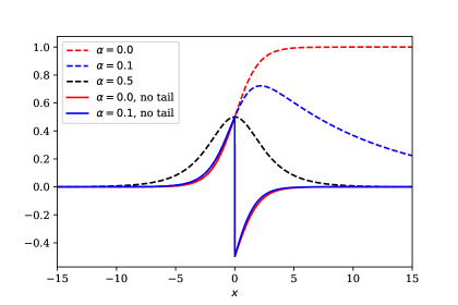
Figure 1: Illustration of $\Lambda(\tau,\Omega)$ evaluation problem. Dashed lines: Integrand from (13) for different values of $\alpha=\tau/\beta$. Solid lines: The same integrand with the tail contribution $t_{\alpha}(x)$ subtracted.

For each $\alpha_{m}=\tau_{m}/\beta$, the integrals $S^{-}_{\alpha}(z)$ and $S^{+}_{\alpha}(z)$ are expressed in terms of special functions or rapidly convergent series and are precomputed on a uniform grid with a fixed number of $z$-points. The precomputed values provide data to construct the cubic spline interpolation between those points, and $T_{\alpha}(z)$ are simple analytical functions that are quick to evaluate. The length of the segment, on which the splines are defined, is chosen such that functions $S^{\pm}_{\alpha}(z)$ can be considered constant outside it. Appendix C contains relevant expressions and necessary implementation details for all observable kinds.

A somewhat similar approach is taken to evaluate integrated Legendre kernels. Once again, let us take the fermionic GF as an example (upper right cell of Table 1),

$$\Lambda(\ell;\Omega)=-\int\limits_{0}^{\Omega}\frac{\beta\sqrt{2\ell+1}(-\mathrm{sgn}(\epsilon))^{\ell}i_{\ell}\left(\frac{\beta|\epsilon|}{2}\right)}{2\cosh(\beta\epsilon/2)}d\epsilon=(-\mathrm{sgn}(\Omega))^{\ell+1}\sqrt{2\ell+1}\int\limits_{0}^{|\Omega|\beta/2}\frac{i_{\ell}(x)}{\cosh(x)}dx,$$ (17)

where $i_{\ell}(x)$ is the modified spherical Bessel function of the first kind [45]. The integrand $\frac{i_{\ell}(x)}{\cosh(x)}$ is rather inconvenient for numerical evaluation, because both the Bessel function and the hyperbolic cosine grow exponentially. Moreover, the integral itself grows logarithmically for $|\Omega|\beta\to\infty$, which makes naive pre-computation and construction of a spline infeasible. This time, our evaluation scheme is based on the following expansion of the integrand,

$$\frac{i_{\ell}(x)}{\cosh(x)}=\frac{e^{x}}{e^{x}+e^{-x}}\sum_{n=0}^{\ell}(-1)^{n}\frac{a_{n}(\ell+1/2)}{x^{n+1}}+\frac{e^{-x}}{e^{x}+e^{-x}}\sum_{n=0}^{\ell}(-1)^{\ell+1}\frac{a_{n}(\ell+1/2)}{x^{n+1}},$$ (18)

with $a_{n}(\ell+1/2)$ being coefficients of the Bessel polynomials [46],

$$a_{n}(\ell+1/2)=\frac{(\ell+n)!}{2^{n}n!(\ell-n)!}.$$ (19)

For large $x$ (high-energy region), the integrand can be approximated as

$$\frac{i_{\ell}(x)}{\cosh(x)}\approx\sum_{n=0}^{\ell}(-1)^{n}\frac{a_{n}(\ell+1/2)}{x^{n+1}}.$$ (20)

In the low-energy region we do the integral $F^{<}(z)\equiv\int_{0}^{z}\frac{i_{\ell}(x)}{\cosh(x)}dx$ on a fixed $z$-mesh, $z\in[0;x_{0}]$, using the adaptive Simpson’s method. Results of the integration are used to construct a cubic spline interpolation of $F^{<}(z)$. For each $\ell$ the boundary value $x_{0}$ between the low- and high-energy regions is found by comparing values of (18) and (20). In the high-energy region we use the asymptotic form (20) to do the integral,

$$F^{>}(z)|_{z>x_{0}}=F^{<}(x_{0})+\left.\left\{\log(x)+\sum_{n=1}^{\ell}(-1)^{n+1}\frac{a_{n}(\ell+1/2)}{x^{n}n}\right\}\right|_{x_{0}}^{z}.$$ (21)

Implementation details for other Legendre kernels can be found in Appendix D.

The second optimization implemented in SOM consists in aggressive caching of rectangles’ contributions to the integral (2). As it is seen from (3), the integral is a simple sum over all rectangles in a configuration. Thanks to the fact that elementary updates affect at most two rectangles at once, it makes sense to store values of every individual term in the sum. In the proposal phase of an update, evaluation of the integrated kernel is then required only for the affected rectangles. If the update is accepted, contributions of the added/changed rectangles are stored in a special cache and can be reused in a later update. Since the size of a configuration does not typically exceed 100, and $M\leq 1000$, the cache requires only a moderate amount of memory.

Besides the two aforementioned optimizations, SOM can take advantage of MPI parallel execution. Generation of particular solutions is “embarrassingly parallel”, because every solution is calculated in a completely independent manner from the others. When a SOM calculation is run in the MPI context, the accumulation of particular solutions is dynamically distributed among available MPI ranks.

4 Usage

4.1 Basic usage example

Running SOM to analytically continue input data requires writing a simple Python script. This usage method is standard for TRIQS applications. We refer the reader to Sec. 9.3 of [1] for instructions on how to execute Python scripts in the TRIQS environment. Details of the script will vary depending on the physical observable to be continued, and its representation. Nonetheless, a typical script will have the following basic parts.

• Import TRIQS and SOM Python modules.

  ⬇

  from pytriqs.gf.local import *

  # HDFArchive interface to HDF5 files.

  from pytriqs.archive.hdf_archive import HDFArchive, HDFArchiveInert

  # HDF5 archives must be modified only by one MPI rank.

  # is_master_node() checks we are on rank 0.

  from pytriqs.utility.mpi import is_master_node

  # bcast() broadcasts its argument from the master node to all others

  from pytriqs.utility.mpi import bcast

  # Main SOM class.

  from pytriqs.applications.analytical_continuation.som import Som

• Load the observable to be continued from an HDF5 archive.

  ⬇

  arch = HDFArchive(’input.h5’, ’r’) if is_master_node() else HDFArchiveInert()

  # Read input Green’s function and broadcast it to all nodes.

  # arch[’g’] must be an object of type GfImTime, GfImFreq or GfLegendre.

  g = bcast(arch[’g’])

  This step can be omitted or modified if the input data comes from a different source. For instance, it could be loaded from text files or generated in the very same script by a quantum Monte-Carlo impurity solver, such as TRIQS/CTHYB [47]. Only the values stored in the g.data array will be used by SOM, while any high frequency expansion information (g.tail) will be disregarded. If g is matrix-valued (or, in TRIQS’s terminology, has a target shape bigger than 1x1), SOM will only construct analytic continuation of the diagonal matrix elements.

• Set the importance function $S(m)$

  ⬇

  S = g.copy()

  # Set all elements of ’S’ to a constant.

  S.data[:] = 1.0

  In this example we assume that all elements of $g(m)$ are equally important. Alternatively, one could read the importance function from an HDF5 archive or another source.

• Construct Som object.

  ⬇

  cont = Som(g, S, kind = "FermionGf", norms = 1.0)

  The argument kind must be used to specify the kind of the physical observable in question. Its recognized values are FermionGf (Green’s function of fermions), BosonCorr (correlator of boson-like operators), BosonAutoCorr (autocorrelator of a Hermitian operator), ZeroTemp (zero temperature correlator). The optional argument norms is a list containing expected norms $\mathcal{N}$ (Eq. 3) of the spectral functions to be found, one positive real number per one diagonal element of g. Instead of setting all elements of norms to the same constant x, one may simply pass norms = x. By default, all norms are set to 1, which is correct for the fermionic Green’s functions. However, adjustments would normally be needed for self-energies and bosonic correlators/autocorrelators.

• Set simulation parameters.

  ⬇

  params = {}

  # SOM will construct a spectral function

  # within this energy window (mandatory)

  params[’energy_window’] = (-5.0,5.0)

  # Number of particular solutions to accumulate (mandatory).

  params[’l’] = 1000

  # Set verbosity level to the maximum on MPI rank 0,

  # and silence all other ranks

  params[’verbosity’] = 3 if is_master_node() else 0

  # Do not auto-adjust the number of particular solutions to accumulate

  # (default and recommended).

  params[’adjust_l’] = False

  # Do not auto-adjust the number of global updates (default and recommended).

  params[’adjust_f’] = False

  # Number of global updates per particular solution.

  params[’f’] = 200

  # Number of local updates per global update.

  params[’t’] = 500

  # Accumulate histogram of the objective function values,

  # useful to analyse quality of solutions.

  params[’make_histograms’] = True

  In Section 4.2 we provide a table of main accepted simulation parameters.

• Run simulation.

  This function call is normally the most expensive part of the script.

• Extract solution and reconstructed input.

  ⬇

  g_w = GfReFreq(window = (-5.0, 5.0), n_points = 1000, indices = g.indices)

  g_w << cont

  # Imaginary time/frequency/Legendre data reconstructed from the solution.

  g_rec = g.copy()

  g_rec << cont

  g_w is the retarded fermionic Green’s function of the real frequency corresponding to the input g. Its imaginary part is set to $-\pi A(\epsilon)$, whereas the real part is computed semi-analytically using the Kramers–Kronig relations (there are closed form expressions for a contribution of one rectangle to the real part). The relation between g_w and $A(\epsilon)$ slightly varies with the observable type; relevant details are to be found in the online documentation.

  The high frequency expansion coefficients will be computed from the sum-of-rectangles representation of $A(\epsilon)$ and written into g_w as well. If g_w is constructed with a wider energy window compared to that from params, $A(\epsilon)$ is assumed to be zero at all “excessive” energy points.

  The reconstructed function g_rec is the result of the substitution of $A(\epsilon)$ back into the integral equation (2). The correctness of results should always be controlled by comparing g with g_rec.

• Save results to an HDF5 archive.

  ⬇

  if mpi.is_master_node():

  with HDFArchive("results.h5",’w’) as ar:

  ar[’g’] = g

  ar[’g_w’] = g_w

  ar[’g_rec’] = g_rec

  # Save histograms for further analysis

  ar[’histograms’] = cont.histograms

The output archive can be read by other TRIQS scripts and outside utilities, in order to analyse, post-process and visualize the resulting spectra. More elaborate examples of SOM Python scripts can be found on the official documentation page, http://krivenko.github.io/som/documentation.html.

4.2 Simulation parameters

Table (2) contains main simulation parameters understood by run() method of class Som. More advanced parameters intended for experienced users are listed in Appendix A.

Parameter Name	Python type	Default value	Meaning
energy_window	(float,float)	N/A	Lower and upper bounds of the energy window. Negative values of the lower bound will be reset to 0 in BosonAutoCorr and ZeroTemp modes.
max_time	int	-1 (unlimited)	Maximum run() execution time in seconds.
verbosity	int	2 on MPI rank 0, 0 otherwise	Verbosity level (maximum level — 3).
t	int	50	Number of elementary updates per global update ($T$). Bigger values may improve ergodicity.
f	int	100	Number of global updates ($F$). Bigger values may improve ergodicity. Ignored if adjust_f=True.
adjust_f	bool	False	Adjust the number of global updates automatically.
l	int	2000	Number of particular solutions to accumulate ($L$). Bigger values reduce the sawtooth noise in the final solution. Ignored if adjust_l=True.
adjust_l	bool	False	Adjust the number of accumulated particular solutions automatically.
make_histograms	bool	False	Accumulate histograms of objective function values.

Table 2: Main run() parameters.

5 Illustrational results

5.1 Testing methodology

We apply SOM to a few synthetic test cases where the exact spectral function is known. These tests serve as an illustration of SOM’s capabilities and as guidance to the prospective users. Being based on a Markov chain algorithm with a fair number of adjustable parameters, SOM may suffer from ergodicity problems and produce characteristic spectral artefacts if the parameters are not properly chosen. It is therefore instructive to consider analytic continuation problems that can potentially pose difficulty to SOM, and study the effect of the various input parameters on the quality of the solution. Throughout this section, we use arbitrary units for all energies and frequencies ($\hbar=1$), while imaginary time $\tau$ and inverse temperature $\beta$ are measured in $[a.u.^{-1}]$.

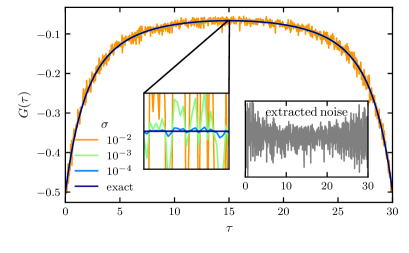
Figure 2: Extraction of noise from the imaginary time Green’s function $G(\tau)$ computed by TRIQS/CTHYB QMC solver, and its subsequent rescaling.

To perform most of the tests, we have devised a special procedure allowing to model stochastic noise characteristic to fermionic Green’s functions $G(\tau)$ measured by QMC solvers. The procedure involves running a single-loop DMFT[5] calculation for a non-interacting single-band tight-binding model on a Bethe lattice using the TRIQS/CTHYB solver. The exact Green’s function of this model $G_{\text{Bethe}}^{\text{ex}}(\tau)$ is easily computed from the well known semi-elliptic spectral function. The impurity solver will introduce some noise $\tilde{\eta}(\tau)$ that can easily be estimated from the accumulation result $G_{\text{Bethe}}^{\text{MC}}(\tau)$ as

$$\tilde{\eta}(\tau)=G_{\text{Bethe}}^{\text{MC}}(\tau)-G_{\text{Bethe}}^{\text{ex}}(\tau),$$ (22)

and normalized according to

$$\eta(\tau)=\tilde{\eta}(\tau)\left/\sqrt{\frac{1}{M}\sum_{m}\left(\tilde{\eta}(\tau_{m})-\frac{1}{M}\sum_{m^{\prime}}\tilde{\eta}(\tau_{m^{\prime}})\right)^{2}}\right..$$ (23)

We ensure that values of the noise are uncorrelated between different time slices $\tau_{m}$ by taking a sufficiently large number of Monte Carlo updates per measurement. Eventually, the extracted and normalized noise is rescaled and added to a model Green’s function to be continued with SOM (Fig. 2),

$$G^{\text{noisy}}_{\sigma}(\tau)=G^{\text{ex}}(\tau)+\sigma\eta(\tau).$$ (24)

By using the described procedure, we hope to reproduce a more realistic noise distribution and its dependence on $\tau$ observed in QMC runs, as compared to a synthetically generated Gaussian noise with a fixed dispersion.

In the case of a susceptibility (two-pole model, see below), we simply add Gaussian noise to $\chi(i\nu_{m})$. It is independently generated for each $\nu_{m}$ with zero mean and equal dispersion $\sigma$.

5.2 Comparison of model spectra

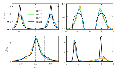
Figure 3: Spectral functions produced by SOM with $F=1500$ depending on the input noise level $\sigma$. The corresponding models are the Hubbard atom (top left), the double Bethe lattice (top right), an asymmetric metal (bottom left), and the zero-temperature Fermi polaron (bottom right). The frequency positions of the asymmetric metal’s superposed Lorentzians are marked by dashed lines.

Results of tests with four model spectra and various levels of added noise are shown in Fig. 3. In all tests presented in that figure, the inverse temperature has been set to $\beta=30$ ($\tau_{max}=30$ for the zero-temperature kernel). All curves have been calculated from the imaginary time input data on a grid with $500$ $\tau$-points ($G^{\text{ex}}(\tau)$ are computed from analytically known spectral functions via (2)). The importance function has been chosen to be a constant in all simulations. The number of global updates is set to $F=1500$ and the number of elementary updates is $T=250$. The remaining parameters are set to SOM defaults, if not stated otherwise.

The model studied first is the single Hubbard atom with the Coulomb repulsion strength $U=2$ at half-filling. Its spectral function comprises two discrete levels at $\pm U/2$ corresponding to excitations through empty and doubly occupied states. For a general complex frequency $z$, the Green’s function of the Hubbard atom reads

$$G(z)=\frac{1/2}{z+U/2+i\delta}+\frac{1/2}{z-U/2+i\delta},$$ (25)

where $\delta=0.1$ is the resonance broadening term. The analytic continuation with SOM shows that strong noise smears the calculated spectral function, the peak height is diminished and the spectral weight is spread asymmetrically around the peak. The smearing at large frequencies is more pronounced. The peak position converges correctly to the exact solution as $\sigma$ decreases.

The second model is the non-interacting double Bethe lattice [48],

$$G(z)=\zeta(z-t_{\perp})+\zeta(z+t_{\perp}),$$ (26)

$$\zeta(z)=\frac{z-i\operatorname{sign}\Im(z)\sqrt{4t_{b}^{2}-z^{2}}}{2t_{b}^{2}}.$$ (27)

The specific feature of this model is a gapped symmetric spectrum with sharp band edges. Splitting between the semi-elliptic bands is given by $|2t_{\perp}|=2$, and their bandwidths are $4t_{b}=1$. Top right part of Fig. 3 shows that at large $\sigma$ the particle–hole asymmetry introduced by the noise can also break the symmetry of the solution. As the noise level goes down, the SOM solution approaches the exact one, but the shape of the bands remains somewhat Lorentzian-like, which leads to an underestimated gap.

As an example of a gapless spectrum (Fig. 3, bottom left), we take a Green’s function that produces a sum of four Lorentzian peaks, i.e.

$$G(z)=\sum_{i}\frac{c_{i}}{z-b_{i}+i\delta}$$ (28)

with $c=\left(0.1,0.4,0.4,0.1\right)$, $b=\left(-0.3,0,0.05,0.3\right)$ and $\delta=0.1$. The Lorentzians overlap and form a single peak that has two shoulders. The peak doesn’t have a mirror symmetry with respect to the vertical axis and its centre is not at the Fermi level. The shoulders are not resolved for the largest noise level of $\sigma=10^{-2}$, but for smaller noise levels $\sigma\in\{10^{-3},10^{-4}\}$ both shoulders are correctly detected by SOM. The spectra with $\sigma\in\{10^{-3},10^{-4}\}$ look notably more noisy. The origin of this effect is SOM’s ability to find the best particular solution that is a very good fit to the input data (with a very small $D_{\text{min}}$). With a fixed $D[A]/D_{\text{min}}$ threshold, only a few particular solutions are considered for inclusion in the final solution. Hence, the less smooth curves.

The fourth model (Fig. 3, bottom right) appears in the context of the Fermi polaron problem, and it has previously been used in [35] to assess performance of other continuation methods. It consists of two peaks modelled via Gaussians,

$$G(z)=\frac{1}{N}\sum_{i}c_{i}e^{-\frac{(z-a_{i})^{2}}{b_{i}}}$$ (29)

with $c=\left(0.62,0.41\right)$, $a=\left(0.74,2.93\right)$ and $b=\left(0.12,0.064\right)$. $N$ is used to set the spectral norm to $1$. Here, we apply the zero-temperature imaginary time kernel with $\tau_{max}=30$. This case is difficult as it contains sharp features over a broad energy range. We observe that the low-energy peak can be relatively well resolved. However, the high-energy peak is strongly broadened with the width dependent of the noise level. Positions of both peaks are reproduced with a reasonable accuracy of $\sim 5\%$.

5.3 Effect of $F$

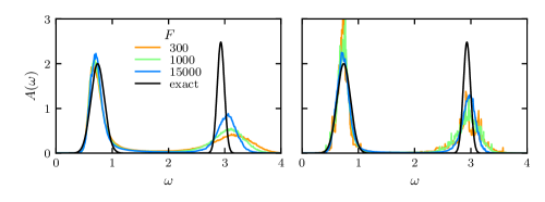
Figure 4: Effect of the number of global updates $F$ on the spectral functions produced by SOM. Shown are spectral functions for the Fermi polaron model obtained from the imaginary time (left) and Legendre (right) input data.

We have observed in practical calculations that the choice of the amount of global updates $F$ can drastically affect ergodicity of SOM Markov chains and, eventually, the output spectra. Fig. 4 shows evolution of SOM spectral functions with $F$ for the Fermi polaron model. Parameters other than $F$ are kept at their default values, i.e. $T=50$, $L=2000$, and the noise level is set to $\sigma=10^{-4}$. The Fermi polaron spectra obtained from the imaginary time representation (Fig. 4, left) demonstrates that SOM has generally no problem resolving the low-energy peak regardless of $F$. The high-energy peak, however, significantly changes its shape and position as $F$ grows, slowly approaching the reference curve.

The situation is rather different, when the Legendre representation is used (Fig. 4, right). As before, the noise is created and added to the Green’s function in the imaginary time representation. Subsequently, it is transformed to the Legendre basis and passed to SOM. The number of Legendre coefficients used here is $N_{\ell}=50$. Positions of both peaks do not change much with $F$. For sufficiently large $F$, their width and height are visibly closer to the exact solution as compared to the imaginary time results. A likely cause of this difference is the truncation of the Legendre expansion and the corresponding noise filtering. In contrast, for small $F$ the peaks contain relatively strong noise. This effect has been found with the asymmetric metal model for large $\sigma$, too. It occurs when the final solution is dominated by a few particular solutions with very small $D$, i.e. when Markov chains suffer from poor ergodicity and struggle to escape an isolated deep minimum of the objective function.

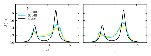
Figure 5: Effect of the number of global updates $F$ on the spectral functions produced by SOM. Shown are spectral functions for the two-pole model obtained from the Matsubara frequency (left) and Legendre (right) input data.

In Fig. 5, a similar comparison is presented for the two-pole susceptibility model[36],

$$\chi(z)=\frac{1}{\chi_{0}}\sum_{i}\frac{c_{i}}{z^{2}-b^{2}_{i}},$$ (30)

$$\chi_{0}=-\sum_{i}\frac{c_{i}}{b^{2}_{i}},$$

with $c=\left(0.1,0.335663\right)$, $b=\left(0.7,1.2\right)$. We use the Hermitian autocorrelator kernel for Matsubara frequencies and add uncorrelated Gaussian noise with the standard deviation $\sigma=10^{-4}$. Other parameters are $\beta=50$, $T=50$ and $L=2000$. For the same number of global updates, we obtain a double-peak structure (Fig. 5, left) similar to that shown in Fig. 2 of [36]. Additionally, we transform the same set of noisy input data into the Legendre representation ($N_{\ell}=50$) and apply the corresponding kernel (Fig. 5, right). As in the case of the Fermi polaron, use of the Legendre basis results in slightly more pronounced peaks. However, their positions are reproduced slightly better by the Matsubara kernel.

5.4 Diagnostics

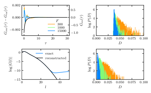
Figure 6: Top, left: Colourful lines/left axis show the difference of the SOM-reconstructed Green’s function and the exact Green’s function of the Fermi polaron model, continued using the imaginary time kernel. Black curve/right axis shows the exact Green’s function itself. Bottom, left: The reconstructed Green’s function and the exact Green’s function in the Legendre basis (same model, $F=15000$). Right: Corresponding histograms of objective function values.

After a solver run, SOM does not only provide the continued function, but also the reconstructed input function as well as a histogram of the objective function. These features are mainly for debugging purposes and for an estimation of result’s quality. It is obvious that the reconstructed Green’s function should ideally be a smooth version of the input Green’s function. In the upper left part of Fig. 6 we plot the difference between the exact Green’s function of the Fermi polaron model and its SOM reconstruction after an imaginary time simulation (the corresponding spectrum is shown in Fig. 4). First of all, we observe that the difference shrinks with increasing $F$. Furthermore, the main difference comes from the small imaginary times. The Green’s function has its largest values there, and so does the noise. At larger $\tau$-points it has less pronounced features or is even featureless. However, $\tau_{\text{max}}$ has to be set sufficiently large, i.e. the result should converge and be independent of its actual value.

The Legendre basis has been identified as a useful tool to filter noise by cutting off large expansion coefficients.[19] In Fig. 6 (bottom left) we provide a similar comparison of exact and reconstructed Green’s functions in the Legendre representation. They lie on top of each other everywhere except for large-order Legendre coefficients. This kind of plots may give a hint at how many Legendre polynomial coefficients should be retained to filter out the noise without losing relevant information in the input data.

The objective function histogram helps determine whether the choice of $F$ and $T$ is adequate. The histogram is usually stretched when $T$ and/or $F$ are too small, and should converge to a sharper peak shape for larger values. Objective function histograms for both used kernels are plotted in the right part of Fig. 6. It is clearly seen that increased $F$ lead to localization of the histograms and, as a result, to more efficient accumulation of particular solutions.

5.5 Final remarks

In conclusion, we would like to make some remarks about the rest of the main simulation parameters. The energy window must be chosen such that the entire spectral weight fits into it, but within the same order of magnitude with the bandwidth. Extremely wide energy windows may be wasteful as they are likely to cause low acceptance rates in the Markov chains. The effect of increased $L$ has not been explicitly studied here, but it is similar to that of a moving average noise filter. It is, however, not recommended to post-process (smoothen) SOM-generated spectra using such a filter, because it can cause artefacts that also depend on the moving frame size. Regarding efficiency, it is worth noting that simulations with the Legendre kernels typically require less CPU time, mainly because of the different dimensions of the input data arrays (a few dozen Legendre coefficients versus $10^{2}-10^{3}$ $\tau$-points/Matsubara frequencies). To give the reader a general idea of how expensive SOM simulations are, we roughly estimated the CPU time required to produce some plots in this section. It took 136 core-hours to obtain one spectral curve for the Hubbard atom, the double Bethe lattice, and the asymmetric metal (Fig. 3). The Fermi polaron simulations were a lot cheaper, 19 core-hours. The most expensive curve ($F=15000$) in Fig. 4 took 20 core-hours with the imaginary time kernel, and 8 core-hours with the Legendre kernel. Similarly, the $F=60000$ curve of Fig. 5 required $25$ and $14$ core-hours with the imaginary time and the Legendre kernels respectively. The required run time scales nearly linearly with $F$.

6 Getting started

6.1 Obtaining SOM

The SOM source code is available publicly and can be obtained from a GitHub repository located at https://github.com/krivenko/som. It is recommended to always use the ‘master’ branch of the repository, as it contains the most recent bug fixes and new features being added to SOM.

6.2 Installation

The current version of SOM requires the TRIQS library 1.4.2 as a prerequisite. An installation procedure of TRIQS is outlined in Sec. 9.2 of [1]. More detailed step-by-step instructions are available on the TRIQS documentation website (https://triqs.github.io/triqs/1.4/install.html). It is of crucial importance to check out the version tag 1.4.2 before compiling and installing TRIQS. This can be done by running the following shell command

$ git checkout 1.4.2

in the cloned source directory of the TRIQS library. It is also important to make sure that TRIQS is compiled against a recent version of the Boost C++ libraries, 1.58 or newer.

Installing SOM is similar to that of other TRIQS-based applications. Assuming that TRIQS 1.4.2 has been installed at /path/to/TRIQS/install/dir SOM is simply installed by issuing the following commands at the shell prompt:

$ git clone https://github.com/krivenko/som som_src
$ mkdir som_build && cd som_build
$ cmake -DTRIQS_PATH=/path/to/TRIQS/install/dir ../som_src
$ make
$ make test
$ make install

This will install SOM in the same location as TRIQS. Further installation instructions are given in the online documentation.

6.3 Citation policy

TRIQS/SOM is provided free of charge. We kindly ask to help us with its continued maintenance and development by citing the present paper, as well as the accompanying paper to the TRIQS library [1], in any published work using the SOM package. We also strongly recommend to cite [34] as the original work where the Stochastic Optimization Method was first introduced.

6.4 Contributing

TRIQS/SOM is an open source project and we encourage feedback and contributions from the user community. Issues should be reported via the GitHub website at https://github.com/krivenko/som/issues. For contributions, we recommend to use the pull requests on the GitHub website. It is recommended to coordinate with the TRIQS/SOM developers before any major contribution.

7 Summary

We have presented the open-source TRIQS/SOM package that implements the Stochastic Optimization Method for analytic continuation. On a set of practical examples, we demonstrated the versatility of TRIQS/SOM, as well as its potential to become a viable alternative to various implementations of the Maximum Entropy Method, the current de facto standard in the field of computational condensed matter physics. The algorithm contains a number of performance optimizations that significantly reduce overall computation costs.

Our plans for future releases include porting the code base to more recent versions of the TRIQS library and adding support for more integral kernels, such as kernels for superconducting correlators [30]. Another interesting addition would be the ability to compute the two-point correlators of particular solutions $\sigma_{mm^{\prime}}$ as defined in [35]. Following the methodology of Goulko et al, one could use the accumulated correlators to characterize the accuracy of the output spectral functions.

8 Acknowledgements

Authors are grateful to Alexander Lichtenstein and Olga Goulko for fruitful discussions, to Roberto Mozara for his valuable comments on the usability of the code, and to Andrey Mishchenko for giving access to the original FORTRAN implementation of the SOM algorithm. We would also like to thank Vladislav Pokorný and Hanna Terletska, who stimulated writing of this paper. I.K. acknowledges support from Deutschen Forschungsgemeinschaft (DFG) via project SFB668 (subproject A3, “Electronic structure and magnetism of correlated systems”). M.H. acknowledges financial support by the DFG in the framework of the SFB925. The computations were performed with resources provided by the North-German Supercomputing Alliance (HLRN).

Appendix A Advanced simulation parameters

Parameter Name	Python type	Default value	Meaning
random_seed	int	34788+928374*MPI.rank	Seed for pseudo-random number generator.
random_name	str	"mt19937" (Mersenne Twister 19937 generator)	Name of pseudo-random number generator. Other supported values are mt11213b, ranlux3 and variants of lagged_fibonacci PRNG (see documentation of Boost.Random for more details).
max_rects	int	60	Maximum number of rectangles to represent a configuration ($K$).
min_rect_width	float	1e-3	Minimal allowed width of a rectangle, in units of the energy window width.
min_rect_weight	float	1e-3	Minimal allowed weight of a rectangle, in units of the requested solution norm $\mathcal{N}$.
distrib_d_max	float	2.0	Maximal parameter of the power-law distribution function for the Metropolis algorithm ($d_{\text{max}}$).
gamma	float	2.0	Proposal probability parameter $\gamma$ (see Appendix E).
adjust_l_good_d	float	2.0	Maximal ratio $D/D_{\text{min}}$ for a particular solution to be considered good, $\alpha_{\text{good}}$ (see Section 2.2).
hist_max	float	2.0	Right boundary of the histograms, in units of $D_{\text{min}}$ (left boundary is always set to $D_{\text{min}}$).
hist_n_bins	int	100	Number of bins for the histograms.

Table 3: Fine tuning run() parameters.

Parameter Name	Python type	Default value	Meaning
adjust_f_range	(int,int)	(100,5000)	Search range for the $F$-adjustment procedure (see Appendix F).
adjust_f_l	int	20	Number of particular solutions used in the $F$-adjustment procedure (see Appendix F).
adjust_f_kappa	float	0.25	Limiting value of $\kappa$ used in the $F$-adjustment procedure (see Appendix F).
adjust_l_range	(int,int)	(100,2000)	Search range for the $L$-adjustment procedure (see Section 2.2).
adjust_l_verygood_d	float	4.0/3	Maximal ratio $D/D_{\text{min}}$ for a particular solution to be considered very good, $\alpha_{\text{very good}}$(see Section 2.2).
adjust_l_ratio	float	0.95	Critical ratio $L_{\text{very good}}/L_{\text{good}}$ that stops the $L$-adjustment procedure (see Section 2.2).

Table 4: run() parameters for $F$- and $L$-adjustment procedures (see Appendix F and Section 2.2 respectively).

Appendix B Evaluation of integrated Matsubara kernels

Observable kind, $O$	Integrated kernel, $\int_{\epsilon_{\mathrm{min}}}^{\epsilon_{\mathrm{max}}}d\epsilon\ K(\xi_{n},\epsilon)R_{\{c,w,h\}}(\epsilon)$
Green’s function of fermions	$h\log\left(\frac{i\omega_{n}-c+w/2}{i\omega_{n}-c-w/2}\right)$
Correlator of boson-like operators	$\frac{hw}{\pi}+\frac{hi\nu_{n}}{\pi}\log\left(\frac{i\nu_{n}-c-w/2}{i\nu_{n}-c+w/2}\right)$
Autocorrelator of a Hermitian operator	$\frac{2hw}{\pi}+\frac{2h\nu_{n}}{\pi}\left(\operatorname{atan}\left(\frac{c-w/2}{\nu_{n}}\right)-\operatorname{atan}\left(\frac{c+w/2}{\nu_{n}}\right)\right)$
Zero temperature correlator	$h\log\left(\frac{iz_{n}-c+w/2}{iz_{n}-c-w/2}\right)$, with $z_{n}=\pi(2n+1)/\tau_{\text{max}}$ or $2\pi n/\tau_{\text{max}}$

Table 5: Integrated kernels in the Matsubara representation. Respective kernels $K(\xi_{n},\epsilon)$ are defined in the second column of Table 1. $R_{\{c,w,h\}}(\epsilon)$ is the rectangle function defined in (9).

Appendix C Evaluation of integrated imaginary time kernels

The spline interpolation procedure used to evaluate the integrated kernels is outlined in Sec. 3. Here we only give the observable-specific details. Throughout this Appendix, we denote dimensionless imaginary time and energy arguments by $\alpha=\tau/\beta=1-\bar{\alpha}$ and $z=\Omega\beta$ respectively. $T_{\alpha}(z)=\int_{0}^{z}t_{\alpha}(x)dx$ denotes the integrated tail contribution. All series found in the tables below are rapidly (exponentially) convergent. $\mathrm{Li}_{2}(x)$ is the dilogarithm (Spence’s function), $\psi(x)=\frac{d}{dx}\log\Gamma(x)$ is the digamma function, $\psi^{(1)}(x)=\frac{d^{2}}{dx^{2}}\log\Gamma(x)$ is the trigamma function, $\Psi(x)=\frac{1}{2}[\psi(\frac{1+x}{2})-\psi(\frac{x}{2})]$.

C.1 Green’s function of fermions

$$\Lambda(\tau;\Omega)=-\frac{1}{\beta}\int\limits_{0}^{z}\frac{e^{-\alpha x}}{1+e^{-x}}dx=-\frac{1}{\beta}\left[\theta(-z)S^{-}_{\alpha}(z)+\theta(z)S^{+}_{\alpha}(z)+T_{\alpha}(z)\right],$$ (31)

$$S^{-}_{\alpha}(z)=-\int\limits_{z}^{0}\left[\frac{e^{-\alpha x}}{1+e^{-x}}-t_{\alpha}(x)\right]dx,\quad S^{+}_{\alpha}(z)=\int\limits_{0}^{z}\left[\frac{e^{-\alpha x}}{1+e^{-x}}-t_{\alpha}(x)\right]dx.$$ (32)

Segments to construct the splines on:

$$S^{-}_{\alpha}(z):z\in[-z_{0},0],\quad S^{+}_{\alpha}(z):z\in[0;z_{0}],\quad z_{0}=-2\log(\mathtt{tolerance}).$$ (33)

$\alpha$	$t_{\alpha}(x)$	$T_{\alpha}(z)$	$S_{\alpha}^{-}(z)$	$S_{\alpha}^{+}(z)$
$0$	$\theta(x)$	$\theta(z)z$	$\log(1+e^{z})-\log(2)$	$\log(1+e^{-z})-\log(2)$
$(0;1/2)$	$\theta(x)e^{-\alpha x}$	$\theta(z)\frac{e^{-\alpha z}-1}{-\alpha}$	$\begin{aligned} \sum_{n=0}^{\infty}(-1)^{n}\frac{e^{(n+\bar{\alpha})z}}{(n+\bar{\alpha})}\\ -\Psi(\bar{\alpha})\end{aligned}$	$\begin{aligned} -\sum_{n=0}^{\infty}(-1)^{n}\frac{e^{-(n+1+\alpha)z}}{-(n+1+\alpha)}\\ -\Psi(1+\alpha)\end{aligned}$
$1/2$	$0$	$0$	$2\operatorname{atan}(e^{z/2})-\pi/2$	$-2\operatorname{atan}(e^{-z/2})+\pi/2$
$(1/2;1)$	$\theta(-x)e^{\bar{\alpha}x}$	$\theta(-z)\frac{e^{\bar{\alpha}z}-1}{\bar{\alpha}}$	$\begin{aligned} -\sum_{n=0}^{\infty}(-1)^{n}\frac{e^{(n+1+\bar{\alpha})z}}{(n+1+\bar{\alpha})}\\ +\Psi(1+\bar{\alpha})\end{aligned}$	$\begin{aligned} \sum_{n=0}^{\infty}(-1)^{n}\frac{e^{-(n+\alpha)z}}{-(n+\alpha)}\\ +\Psi(\alpha)\end{aligned}$
$1$	$\theta(-x)$	$\theta(-z)z$	$-\log(1+e^{z})+\log(2)$	$-\log(1+e^{-z})+\log(2)$

C.2 Correlator of boson-like operators

$$\Lambda(\tau;\Omega)=\frac{1}{\pi\beta^{2}}\int\limits_{0}^{z}\frac{xe^{-\alpha x}}{1-e^{-x}}dx=\frac{1}{\pi\beta^{2}}\left[\theta(-z)S^{-}_{\alpha}(z)+\theta(z)S^{+}_{\alpha}(z)+T_{\alpha}(z)\right],$$ (34)

$$S^{-}_{\alpha}(z)=-\int\limits_{z}^{0}\left[\frac{xe^{-\alpha x}}{1-e^{-x}}-t_{\alpha}(x)\right]dx,\quad S^{+}_{\alpha}(z)=\int\limits_{0}^{z}\left[\frac{xe^{-\alpha x}}{1-e^{-x}}-t_{\alpha}(x)\right]dx.$$ (35)

Segments to construct the splines on:

$$S^{-}_{\alpha}(z):z\in[-z_{0},0],\quad S^{+}_{\alpha}(z):z\in[0;z_{0}].$$ (36)

Factor $x$ in the kernel tends to strengthen its delocalization, so it makes sense to choose $z_{0}$ slightly larger, for instance, $z_{0}=-2.3\log(\mathtt{tolerance})$.

$\alpha$	$t_{\alpha}(x)$	$T_{\alpha}(z)$	$S_{\alpha}^{-}(z)$	$S_{\alpha}^{+}(z)$
$0$	$\theta(x)x$	$\theta(z)z^{2}/2$	$\begin{aligned} -\pi^{2}/6+z\log(1-e^{z})\\ +\mathrm{Li}_{2}(e^{z})\end{aligned}$	$\begin{aligned} \pi^{2}/6+z\log(1-e^{-z})\\ -\mathrm{Li}_{2}(e^{-z})\end{aligned}$
$(0;1/2)$	$\theta(x)xe^{-\alpha x}$	$\theta(z)\frac{1-e^{-\alpha z}(1+z\alpha)}{\alpha^{2}}$	$\begin{aligned} \sum_{n=0}^{\infty}\frac{e^{(n+\bar{\alpha})z}[1-z(n+\bar{\alpha})]}{(n+\bar{\alpha})^{2}}\\ -\psi^{(1)}(\bar{\alpha})\end{aligned}$	$\begin{aligned} -\sum_{n=1}^{\infty}\frac{e^{-(n+\alpha)z}[1+z(n+\alpha)]}{(n+\alpha)^{2}}\\ +\psi^{(1)}(1+\alpha)\end{aligned}$
$1/2$	$0$	$0$	$\begin{aligned} -\pi^{2}/2+z\log(\tanh(-z/4))\\ -\mathrm{Li}_{2}(e^{z})+4\mathrm{Li}_{2}(e^{z/2})\end{aligned}$	$\begin{aligned} \pi^{2}/2+z\log(\tanh(z/4))\\ +\mathrm{Li}_{2}(e^{-z})-4\mathrm{Li}_{2}(e^{-z/2})\end{aligned}$
$(1/2;1)$	$\theta(-x)(-x)e^{\bar{\alpha}x}$	$\theta(-z)\frac{e^{\bar{\alpha}z}(1-z\bar{\alpha})-1}{(\bar{\alpha})^{2}}$	$\begin{aligned} \sum_{n=1}^{\infty}\frac{e^{(n+\bar{\alpha})z}[1-z(n+\bar{\alpha})]}{(n+\bar{\alpha})^{2}}\\ -\psi^{(1)}(1+\bar{\alpha})\end{aligned}$	$\begin{aligned} -\sum_{n=0}^{\infty}\frac{e^{-(n+\alpha)z}[1+z(n+\alpha)]}{(n+\alpha)^{2}}\\ +\psi^{(1)}(\alpha)\end{aligned}$
$1$	$\theta(-x)(-x)$	$\theta(-z)(-z^{2}/2)$	$\begin{aligned} -\pi^{2}/6+z\log(1-e^{z})\\ +\mathrm{Li}_{2}(e^{z})\end{aligned}$	$\begin{aligned} \pi^{2}/6+z\log(1-e^{-z})\\ -\mathrm{Li}_{2}(e^{-z})\end{aligned}$

C.3 Autocorrelator of a Hermitian operator

$$\Lambda(\tau;\Omega)=\frac{1}{\pi\beta^{2}}\int\limits_{0}^{z}\frac{x(e^{-\alpha x}+e^{-\bar{\alpha}x})}{1-e^{-x}}dx=\frac{1}{\pi\beta^{2}}\left[S_{\alpha}(z)+T_{\alpha}(z)\right],$$ (37)

$$S_{\alpha}(z)=\int\limits_{0}^{z}\left[\frac{x(e^{-\alpha x}+e^{-(1-\alpha)x})}{1-e^{-x}}-t_{\alpha}(x)\right]dx.$$ (38)

(The upper integration limit can be only positive, which eliminates the need for two splines). Segment to construct the spline on is $z\in[0;z_{0}]$, $z_{0}=-2.3\log(\mathtt{tolerance})$.

$\alpha$	$t_{\alpha}(x)$	$T_{\alpha}(z)$	$S_{\alpha}(z)$
$0,1$	$x(1+e^{-x})$	$1+z^{2}/2-e^{-z}(1+z)$	$\begin{aligned} -1+\pi^{2}/3+2z\log(1-e^{-z})\\ -2\mathrm{Li}_{2}(e^{-z})+e^{-z}(1+z)\end{aligned}$
$(0;1/2)\cup(1/2;1)$	$x(e^{-\alpha x}+e^{-\bar{\alpha}x})$	$\begin{array}[]{c}\frac{1-e^{-\alpha z}(1+z\alpha)}{\alpha^{2}}\\ +\frac{1-e^{-\bar{\alpha}z}(1+z\bar{\alpha})}{(\bar{\alpha})^{2}}\end{array}$	$\begin{aligned} -\sum_{n=1}^{\infty}\frac{e^{-(n+\alpha)z}[1+z(n+\alpha)]}{(n+\alpha)^{2}}+\psi^{(1)}(1+\alpha)\\ -\sum_{n=1}^{\infty}\frac{e^{-(n+\bar{\alpha})z}[1+z(n+\bar{\alpha})]}{(n+\bar{\alpha})^{2}}+\psi^{(1)}(1+\bar{\alpha})\end{aligned}$
$1/2$	$2xe^{-x/2}$	$4(2-e^{-z/2}(2+z))$	$\begin{aligned} -8+\pi^{2}+4e^{-z/2}(2+z)+2z\log\tanh(z/4)\\ -8\mathrm{Li}_{2}(e^{-z/2})+2\mathrm{Li}_{2}(e^{-z})\end{aligned}$

C.4 Zero temperature correlator

$$\int\limits_{0}^{+\infty}d\epsilon\ K(\tau,\epsilon)R_{\{c,w,h\}}(\epsilon)=\begin{cases}-hw,&\tau=0,\\ \frac{h}{\tau}(e^{-\tau(c+w/2)}-e^{-\tau(c-w/2)}),&\mathrm{otherwise}.\end{cases}$$ (39)

Appendix D Evaluation of integrated Legendre kernels

The spline interpolation procedure used to evaluate the integrated kernels is outlined in Sec. 3.

D.1 Green’s function of fermions

$$\Lambda(\ell;\Omega)=(-\mathrm{sgn}(\Omega))^{\ell+1}\sqrt{2\ell+1}\int_{0}^{|\Omega|\beta/2}\frac{i_{\ell}(x)}{\cosh(x)}dx.$$ (40)

Asymptotic form of the integrand ($x\to\infty$),

$$\frac{i_{\ell}(x)}{\cosh(x)} =\frac{e^{x}}{e^{x}+e^{-x}}\sum_{n=0}^{\ell}(-1)^{n}\frac{a_{n}(\ell+1/2)}{x^{n+1}}+\frac{e^{-x}}{e^{x}+e^{-x}}\sum_{n=0}^{\ell}(-1)^{\ell+1}\frac{a_{n}(\ell+1/2)}{x^{n+1}}$$

$$\approx\sum_{n=0}^{\ell}(-1)^{n}\frac{a_{n}(\ell+1/2)}{x^{n+1}}.$$ (41)

Integral $F(z)=\int_{0}^{z}\frac{i_{\ell}(x)}{\cosh(x)}dx$ in the high-energy limit,

$$F^{>}(z)|_{z>x_{0}}=F^{<}(x_{0})+\left.\left\{\log(x)+\sum_{n=1}^{\ell}(-1)^{n+1}\frac{a_{n}(\ell+1/2)}{x^{n}n}\right\}\right|_{x_{0}}^{z}.$$ (42)

D.2 Correlator of boson-like operators

$$\Lambda(\ell;\Omega)=-(-\mathrm{sgn}(\Omega))^{\ell+1}\frac{2\sqrt{2\ell+1}}{\pi\beta}\int_{0}^{|\Omega|\beta/2}\frac{i_{\ell}(x)x}{\sinh(x)}dx.$$ (43)

Asymptotic form of the integrand ($x\to\infty$),

$$\frac{i_{\ell}(x)x}{\sinh(x)} =\frac{e^{x}}{e^{x}-e^{-x}}\sum_{n=0}^{\ell}(-1)^{n}\frac{a_{n}(\ell+1/2)}{x^{n}}+\frac{e^{-x}}{e^{x}-e^{-x}}\sum_{n=0}^{\ell}(-1)^{\ell+1}\frac{a_{n}(\ell+1/2)}{x^{n}}$$

$$\approx\sum_{n=0}^{\ell}(-1)^{n}\frac{a_{n}(\ell+1/2)}{x^{n}}.$$ (44)

Integral $F(z)=\int_{0}^{z}\frac{i_{\ell}(x)x}{\sinh(x)}dx$ in the high-energy limit,

$$F^{>}(z)|_{z>x_{0}}=F^{<}(x_{0})+\left.\left\{x-\frac{\ell(\ell+1)}{2}\log(x)+\sum_{n=1}^{\ell-1}(-1)^{n}\frac{a_{n+1}(\ell+1/2)}{x^{n}n}\right\}\right|_{x_{0}}^{z}.$$ (45)

D.3 Autocorrelator of a Hermitian operator

$$\Lambda(\ell;\Omega)=(1+(-1)^{\ell})\frac{2\sqrt{2\ell+1}}{\pi\beta}\int_{0}^{\Omega\beta/2}\frac{i_{\ell}(x)x}{\sinh(x)}dx.$$ (46)

This integral is evaluated in full analogy with the previous kernel.

D.4 Zero temperature correlator

$$\Lambda(\ell;\Omega)=(-1)^{\ell+1}\sqrt{2\ell+1}\int_{0}^{\Omega\tau_{max}/2}2e^{-x}i_{\ell}(x)dx.$$ (47)

Asymptotic form of the integrand ($x\to\infty$),

$$2e^{-x}i_{\ell}(x)=\sum_{n=0}^{\ell}(-1)^{n}\frac{a_{n}(\ell+1/2)}{x^{n}}+e^{-2x}\sum_{n=0}^{\ell}(-1)^{\ell+1}\frac{a_{n}(\ell+1/2)}{x^{n}}\approx\sum_{n=0}^{\ell}(-1)^{n}\frac{a_{n}(\ell+1/2)}{x^{n}}.$$ (48)

Integral $F(z)=\int_{0}^{z}2e^{-x}i_{\ell}(x)dx$ in the high-energy limit,

$$F^{>}(z)|_{z>x_{0}}=F^{<}(x_{0})+\left.\left\{\log(x)+\sum_{n=1}^{\ell}(-1)^{n+1}\frac{a_{n}(\ell+1/2)}{x^{n}n}\right\}\right|_{x_{0}}^{z}.$$ (49)

Appendix E Probability density function for the parameter change

Every proposed elementary update is parametrized by a real number $\delta\xi\in[\delta\xi_{\mathrm{min}};\delta\xi_{\mathrm{max}}]$. A concrete meaning of $\delta\xi$ depends on the elementary update in question. For instance, $\delta\xi$ can be a shift of the centre of an existing rectangle, or the weight of a rectangle to be added. In general, $\delta\xi$ are defined so that larger $|\delta\xi|$ correspond to more prominent changes in the configuration. SOM randomly generates values of $\delta\xi$ according to the following probability density function,

$$\mathcal{P}(\delta\xi)=N\exp\left(-\gamma\frac{|\delta\xi|}{X}\right),\quad X\equiv\max(|\delta\xi_{\mathrm{min}}|,|\delta\xi_{\mathrm{max}}|),$$ (50)

$$N=\frac{\gamma}{X}\left[\operatorname{sign}(\delta\xi_{\mathrm{min}})(e^{-\gamma|\delta\xi_{\mathrm{min}}|/X}-1)+\operatorname{sign}(\delta\xi_{\mathrm{max}})(1-e^{-\gamma|\delta\xi_{\mathrm{max}}|/X})\right]^{-1}.$$ (51)

User can change parameter $\gamma>0$ to control non-uniformity of the PDF (50).

Appendix F Fit quality criterion and choice of $F$

Mishchenko introduced a special quantity $\kappa$ that characterizes the fit quality of a given particular solution $A(\epsilon)$ [41].

$$\kappa=\frac{1}{M-1}\sum_{m=2}^{M}\theta(-\Delta(m)\Delta(m-1)).$$ (52)

The observable $O$ and, therefore, deviation $\Delta(m)$ (Eq. (6)) are assumed to be real-valued here. $\kappa$ measures the degree to what adjacent deviation values $\Delta(m)$ are anti-correlated. Since input data points $O(\xi_{m})$ are expected to be statistically independent, deviations $\Delta(m)$ should rapidly fluctuate changing sign between adjacent points. Conversely, if the solution $A(\epsilon)$ gives a systematic deviation from the input points $O(\xi_{m})$, products $\Delta(m)\Delta(m-1)$ are more likely to be positive, which results in a smaller $\kappa$. Ideally, $\kappa$ must approach $1/2$, but in practice values as small as $1/4$ signal satisfactory fit quality.

A similar expression can be written for complex-valued observables, such as functions of Matsubara frequencies. Our generalization consists in replacing

$$\theta(-\Delta(m)\Delta(m-1))\mapsto\frac{1}{2}\left[1-\frac{\Re[\Delta(m)\Delta^{*}(m-1)]}{|\Delta(m)\Delta^{*}(m-1)|}\right]\\ =\frac{1}{2}\left[1-\cos[\arg(\Delta(m))-\arg(\Delta(m-1))]\right].$$ (53)

According to the modified definition, two adjacent values of $\Delta$ are considered anti-correlated, if the complex phase shift between them exceeds $\pm\pi/2$. In the case of real-valued quantities the phase shift is always either 0, or $\pi$.

SOM has an option to automatically adjust the number of global updates $F$ used in a calculation. Starting from $F=F_{\text{min}}$ it finds a few (20 by default) particular solutions $\tilde{A}(\epsilon)$ and checks that $\kappa\geq\kappa_{\text{min}}$ (1/4 by default) for at least a half of them. If this is not the case, the test is repeated with an increased $F$. This procedure stops upon a successful $\kappa$-test or when $F_{\text{max}}$ is reached, whichever happens first.

References

-
[1]
O. Parcollet, M. Ferrero, T. Ayral, H. Hafermann, I. Krivenko, L. Messio,
P. Seth,
Triqs:
A toolbox for research on interacting quantum systems, Computer Physics
Communications 196 (2015) 398 – 415.
doi:https://doi.org/10.1016/j.cpc.2015.04.023.
URL http://www.sciencedirect.com/science/article/pii/S0010465515001666 -
[2]
E. Gull, A. J. Millis, A. I. Lichtenstein, A. N. Rubtsov, M. Troyer, P. Werner,
Continuous-time
monte carlo methods for quantum impurity models, Rev. Mod. Phys. 83 (2011)
349–404.
doi:10.1103/RevModPhys.83.349.
URL https://link.aps.org/doi/10.1103/RevModPhys.83.349 -
[3]
W. Metzner, D. Vollhardt,
Correlated
Lattice Fermions in d=∞ Dimensions, Physical Review Letters 62 (3) (1989)
324–327.
doi:10.1103/PhysRevLett.62.324.
URL http://journals.aps.org/prl/abstract/10.1103/PhysRevLett.62.324 -
[4]
A. Georges, G. Kotliar,
Hubbard
model in infinite dimensions, Physical Review B 45 (12) (1992) 6479–6483.
doi:10.1103/PhysRevB.45.6479.
URL http://journals.aps.org/prb/abstract/10.1103/PhysRevB.45.6479 -
[5]
A. Georges, G. Kotliar, W. Krauth, M. Rozenberg,
Dynamical
mean-field theory of strongly correlated fermion systems and the limit of
infinite dimensions, Reviews of Modern Physics 68 (1) (1996) 13–125.
doi:http://dx.doi.org/10.1103/RevModPhys.68.13.
URL http://journals.aps.org/rmp/abstract/10.1103/RevModPhys.68.13 -
[6]
G. Kotliar, S. Savrasov, K. Haule, V. Oudovenko, O. Parcollet, C. Marianetti,
Electronic
structure calculations with dynamical mean-field theory, Reviews of Modern
Physics 78 (3) (2006) 865–951.
doi:10.1103/RevModPhys.78.865.
URL http://link.aps.org/doi/10.1103/RevModPhys.78.865 -
[7]
L. Mühlbacher, E. Rabani,
Real-time path
integral approach to nonequilibrium many-body quantum systems, Phys. Rev.
Lett. 100 (2008) 176403.
doi:10.1103/PhysRevLett.100.176403.
URL https://link.aps.org/doi/10.1103/PhysRevLett.100.176403 -
[8]
P. Werner, T. Oka, A. J. Millis,
Diagrammatic monte
carlo simulation of nonequilibrium systems, Phys. Rev. B 79 (2009) 035320.
doi:10.1103/PhysRevB.79.035320.
URL https://link.aps.org/doi/10.1103/PhysRevB.79.035320 -
[9]
P. Werner, T. Oka, M. Eckstein, A. J. Millis,
Weak-coupling
quantum monte carlo calculations on the keldysh contour: Theory and
application to the current-voltage characteristics of the anderson model,
Phys. Rev. B 81 (2010) 035108.
doi:10.1103/PhysRevB.81.035108.
URL https://link.aps.org/doi/10.1103/PhysRevB.81.035108 -
[10]
H.-T. Chen, G. Cohen, D. R. Reichman,
Inchworm monte carlo for exact
non-adiabatic dynamics. i. theory and algorithms, The Journal of Chemical
Physics 146 (5) (2017) 054105.
doi:10.1063/1.4974328.
URL https://doi.org/10.1063/1.4974328 -
[11]
H.-T. Chen, G. Cohen, D. R. Reichman,
Inchworm monte carlo for exact
non-adiabatic dynamics. ii. benchmarks and comparison with established
methods, The Journal of Chemical Physics 146 (5) (2017) 054106.
doi:10.1063/1.4974329.
URL http://dx.doi.org/10.1063/1.4974329 -
[12]
A. N. Rubtsov, V. V. Savkin, A. I. Lichtenstein,
Continuous-time
quantum monte carlo method for fermions, Phys. Rev. B 72 (2005) 035122.
doi:10.1103/PhysRevB.72.035122.
URL https://link.aps.org/doi/10.1103/PhysRevB.72.035122 -
[13]
P. Werner, A. J. Millis,
Hybridization
expansion impurity solver: General formulation and application to kondo
lattice and two-orbital models, Phys. Rev. B 74 (2006) 155107.
doi:10.1103/PhysRevB.74.155107.
URL https://link.aps.org/doi/10.1103/PhysRevB.74.155107 -
[14]
E. Gull, P. Werner, O. Parcollet, M. Troyer,
Continuous-time
auxiliary-field monte carlo for quantum impurity models, EPL (Europhysics
Letters) 82 (5) (2008) 57003.
URL http://stacks.iop.org/0295-5075/82/i=5/a=57003 -
[15]
J. Otsuki, H. Kusunose, P. Werner, Y. Kuramoto,
Continuous-time quantum monte
carlo method for the coqblinâschrieffer model, Journal of the Physical
Society of Japan 76 (11) (2007) 114707.
doi:10.1143/JPSJ.76.114707.
URL https://doi.org/10.1143/JPSJ.76.114707 -
[16]
N. Prokof’ev, B. Svistunov,
Bold
diagrammatic monte carlo technique: When the sign problem is welcome, Phys.
Rev. Lett. 99 (2007) 250201.
doi:10.1103/PhysRevLett.99.250201.
URL https://link.aps.org/doi/10.1103/PhysRevLett.99.250201 -
[17]
N. V. Prokof’ev, B. V. Svistunov,
Bold diagrammatic
monte carlo: A generic sign-problem tolerant technique for polaron models and
possibly interacting many-body problems, Phys. Rev. B 77 (2008) 125101.
doi:10.1103/PhysRevB.77.125101.
URL https://link.aps.org/doi/10.1103/PhysRevB.77.125101 -
[18]
R. Blankenbecler, D. J. Scalapino, R. L. Sugar,
Monte carlo
calculations of coupled boson-fermion systems. i, Phys. Rev. D 24 (1981)
2278–2286.
doi:10.1103/PhysRevD.24.2278.
URL https://link.aps.org/doi/10.1103/PhysRevD.24.2278 -
[19]
L. Boehnke, H. Hafermann, M. Ferrero, F. Lechermann, O. Parcollet,
Orthogonal
polynomial representation of imaginary-time green’s functions, Phys. Rev. B
84 (2011) 075145.
doi:10.1103/PhysRevB.84.075145.
URL https://link.aps.org/doi/10.1103/PhysRevB.84.075145 -
[20]
C. W. Groetsch, Integral
equations of the first kind, inverse problems and regularization: a crash
course, Journal of Physics: Conference Series 73 (1) (2007) 012001.
URL http://stacks.iop.org/1742-6596/73/i=1/a=012001 - [21] H. J. Vidberg, J. W. Serene, Solving the eliashberg equations by means of n-point padé approximants, Journal of Low Temperature Physics 29 (1977) 179–192. doi:10.1007/BF00655090.
-
[22]
X. Zhu, G. Zhu,
A
method for directly finding the denominator values of rational interpolants,
Journal of Computational and Applied Mathematics 148 (2) (2002) 341 – 348.
doi:https://doi.org/10.1016/S0377-0427(02)00554-X.
URL http://www.sciencedirect.com/science/article/pii/S037704270200554X -
[23]
K. S. D. Beach, R. J. Gooding, F. Marsiglio,
Reliable padé
analytical continuation method based on a high-accuracy symbolic computation
algorithm, Phys. Rev. B 61 (2000) 5147–5157.
doi:10.1103/PhysRevB.61.5147.
URL https://link.aps.org/doi/10.1103/PhysRevB.61.5147 -
[24]
M. Jarrell, J. Gubernatis,
Bayesian
inference and the analytic continuation of imaginary-time quantum monte carlo
data, Physics Reports 269 (3) (1996) 133 – 195.
doi:https://doi.org/10.1016/0370-1573(95)00074-7.
URL http://www.sciencedirect.com/science/article/pii/0370157395000747 -
[25]
R. K. Bryan, Maximum entropy analysis
of oversampled data problems, European Biophysics Journal 18 (3) (1990)
165–174.
doi:10.1007/BF02427376.
URL https://doi.org/10.1007/BF02427376 -
[26]
G. J. Kraberger, R. Triebl, M. Zingl, M. Aichhorn,
Maximum entropy
formalism for the analytic continuation of matrix-valued green’s functions,
Phys. Rev. B 96 (2017) 155128.
doi:10.1103/PhysRevB.96.155128.
URL https://link.aps.org/doi/10.1103/PhysRevB.96.155128 - [27] G. J. Kraberger, M. Zingl, MaxEnt, https://github.com/TRIQS/maxent.
-
[28]
D. Bergeron, A.-M. S. Tremblay,
Algorithms for
optimized maximum entropy and diagnostic tools for analytic continuation,
Phys. Rev. E 94 (2016) 023303.
doi:10.1103/PhysRevE.94.023303.
URL https://link.aps.org/doi/10.1103/PhysRevE.94.023303 - [29] D. Bergeron, TRIQS Interface to the OmegaMaxEnt Code, https://github.com/TRIQS/omegamaxent_interface.
-
[30]
R. Levy, J. LeBlanc, E. Gull,