A Simple Model for Radiative and Convective Fluxes in Planetary Atmospheres

Abstract

One-dimensional (vertical) models of planetary atmospheres typically balance the net solar and internal energy fluxes against the net thermal radiative and convective heat fluxes to determine an equilibrium thermal structure. Thus, simple models of shortwave and longwave radiative transport can provide insight into key processes operating within planetary atmospheres. Here, we develop a simple, analytic expression for both the downwelling thermal and net thermal radiative fluxes in a planetary troposphere. We assume that the atmosphere is non-scattering at thermal wavelengths and that opacities are grey at these same wavelengths. Additionally, we adopt an atmospheric thermal structure that follows a modified dry adiabat as well as a physically-motivated power-law relationship between grey thermal optical depth and atmospheric pressure. To verify the accuracy of our analytic treatment, we compare our model to more sophisticated “full physics” tools as applied to Venus, Earth, and a cloudfree Jupiter, thereby exploring a diversity of atmospheric conditions conditions. Next, we seek to better understand our analytic model by exploring how thermal radiative flux profiles respond to variations in key physical parameters, such as the total grey thermal optical depth of the atmosphere. Using energy balance arguments, we derive convective flux profiles for the tropospheres of all Solar System worlds with thick atmospheres, and propose a scaling that enables inter-comparison of these profiles. Lastly, we use our analytic treatment to discuss the validity of other simple models of convective fluxes in planetary atmospheres. Our new expressions build on decades of analytic modeling exercises in planetary atmospheres, and further prove the utility of simple, generalized tools in comparative planetology studies.

and

Proposed Running Head:
Planetary Radiative and Convective Fluxes

Please send Editorial Correspondence to:

Tyler D. Robinson
Northern Arizona University
Department of Physics and Astronomy
Box 6010
Flagstaff, AZ 86011-6010, USA.

Email: tyler.robinson@nau.edu
Phone: 928-523-0350
Fax: 928-523-1371

1 Introduction

The thermal structure of a planetary atmosphere is determined via complex energy and mass exchanges in radiative, advective, and diffusive processes. One-dimensional (vertical) models of planetary atmospheres seek to explain how radiative processes and the vertical convective transport of heat and condensible species combine to establish the average atmospheric structure of a world. In these one-dimensional planetary climate models, treatments of radiative transport vary in complexity. The most sophisticated radiation tools operate at high spectral resolution (Wordsworth et al., 2017) with full physics treatments of scattering processes (Robinson and Crisp, 2018), or may adopt lower-resolution correlated-$k$ techniques (Goody et al., 1989; Lacis and Oinas, 1991). Alternatively, the simplest models may use a semi-grey two-stream approach (e.g., McKay et al., 1999). Similarly, sophisticated treatments of convective transport can range from applications of planetary boundary layer physics (Mellor and Yamada, 1974) to mixing length models (e.g., Gierasch and Goody, 1968). Less-complex tools apply the relatively straightforward “convective adjustment” approach (Manabe and Strickler, 1964). Many of these topics are discussed in a recent review by Marley and Robinson (2014).

Semi-grey, windowed-grey, and banded-grey radiative transfer techniques have a long history of application to planetary atmospheres (Robinson, 2015). Semi-grey or windowed-grey radiative transfer models have been used to explore the climate of modern and ancient Earth (Hart, 1978; Weaver and Ramanathan, 1995; Frierson et al., 2006; Pelkowski et al., 2008). Similar semi-grey radiative approaches have been applied to studies of both the one-dimensional and three-dimensional structure of Titan’s atmosphere (McKay et al., 1999; Mitchell et al., 2006), as well as to runaway greenhouse worlds (Nakajima et al., 1992).

Beyond the Solar System, the limited atmospheric data available combined with the explosion of interest in exoplanets has driven the need for simple parameterized (Madhusudhan and Seager, 2009) or physically-based (Hubeny et al., 2003; Hansen, 2008) atmospheric thermal structure models. Building on the semi-grey radiative equilibrium solution applied to hot Jupiter exoplanets in Guillot (2010), Parmentier and Guillot (2014) developed a banded-grey “picket fence” radiative equilibrium model that can better reproduce the structure of hot Jupiter stratospheres (Parmentier et al., 2015), where semi-grey radiative equilibrium models tend to overestimate atmospheric temperatures (see explanation in Pierrehumbert, 2011, their Section 4.7). Heng et al. (2012) extensively investigated the application of semi-grey radiative equilibrium models to hot Jupiter atmospheres, and these concepts have subsequently been adapted to include scattering (Heng et al., 2014) and “picket fence” thermal opacities (Mohandas et al., 2018).

Markedly fewer studies have combined grey radiative transfer techniques with treatments of convection. This may seem striking as convection is known to be critical to driving vertical transport, and can be related to effective upwelling windspeeds in planetary tropospheres (Gierasch and Conrath, 1985). In a pair of early examples, Sagan (1969) and Weaver and Ramanathan (1995) investigated the onset of convective instability in semi-grey and windowed-grey atmospheres.

More recently, Ozawa and Ohmura (1997) (and also Wu and Liu, 2010; Herbert et al., 2013) used a semi-grey radiative transfer model to derive convective fluxes for Earth-like conditions under the “maximum entropy production” principle, wherein convective energy transport is postulated to maximize the local entropy production rate. Indeed, Ozawa and Ohmura (1997) showed that temperature profiles computed using the maximum entropy production principle were less steep and had lower surface temperatures than pure radiative equilibrium solutions, thus reproducing behaviors seen in models that adopt other treatments of convection (e.g., Manabe and Strickler, 1964). Lorenz and McKay (2003) used semi-grey radiative transport expressions to heuristically arrive at an analytic expression for the convective flux at a planetary surface, and showed that this expression could reproduce the convective fluxes computed by more complex models. Finally, Robinson and Catling (2012) produced analytic expressions for the thermal structure of a planetary atmosphere with a semi-grey radiative stratosphere overlying a convective troposphere whose structure follows a modified dry adiabat. These authors used this tool to understand the physics behind a common 0.1 bar tropopause pressure seen throughout the Solar System (Robinson and Catling, 2014).

In what follows, we extend the Robinson and Catling (2012) model to include an analytic treatment of downwelling thermal radiative fluxes in a semi-grey atmosphere that includes a convective troposphere, and also introduce more realistic lower boundary conditions to a previous solution for the upwelling thermal radiative flux. Taken together, these expressions for the upwelling and downwelling thermal radiative fluxes yield straightforward, physically-based expressions for both the net thermal flux and the convective heat flux in planetary tropospheres. We validate our net thermal flux treatment against more sophisticated climate and radiative transfer models, and we apply our derived convective heat flux profiles to compare Solar System worlds. Finally, we use our new model to comment on the maximum entropy production approach explored by Ozawa and Ohmura (1997) and on the heuristic convective flux expression given by Lorenz and McKay (2003).

2 Theory

In a one-dimensional, plane-parallel atmosphere, the grey two-stream Schwarzschild equations for non-scattering thermal radiative transport are (Andrews, 2010, p. 84),

$$\frac{dF^{+}}{d\tau}=D\left(F^{+}-\sigma T^{4}\right)\ ,$$ (1)

$$\frac{dF^{-}}{d\tau}=-D\left(F^{-}-\sigma T^{4}\right)\ ,$$ (2)

where $\tau$ is the vertical grey thermal optical depth, $T$ is the temperature, $\sigma$ is the Stefan-Boltzmann constant ($5.67\times 10^{-8}$ W m^-2 K^-4), $D$ is the so-called diffusivity factor, and $F^{+}$ and $F^{-}$ are the upwelling and downwelling thermal radiative fluxes, respectively. Recall that the diffusivity factor accounts for the integration of radiance over a hemisphere, and values spanning 1.5–2 are commonly adopted in the literature (Rodgers and Walshaw, 1966; Armstrong, 1968). Thus, given a temperature profile, $T\left(\tau\right)$, Equations 1 and 2 can be evaluated to yield the upwelling and downwelling thermal radiative flux profiles for an atmosphere. While more sophisticated treatments of closure used to derive the two-stream equations have been detailed (Heng et al., 2014), the extremely simple semi-grey approximation adopted in the present work argues against the need for moving to sophisticated two-stream models.

In the convective portion of a non-condensing atmosphere, the thermal structure follows Poisson’s adiabatic state equation (Catling and Kasting, 2017, their Equation 1.32),

$$T=T_{0}\left(\frac{p}{p_{0}}\right)^{(\gamma-1)/\gamma}\ ,$$ (3)

where $T_{0}$ is a reference temperature at $p_{0}$ (taken to be, e.g., the surface, or the 1 bar pressure level in the atmosphere of a gaseous world), and $\gamma$ is the ratio of specific heats. Following Sagan (1962), we modify the dry adiabat to account for latent heat release or non-constant specific heats by introducing a parameter, $\alpha$, into the adiabatic state equation, giving,

$$T=T_{0}\left(\frac{p}{p_{0}}\right)^{\alpha(\gamma-1)/\gamma}\ .$$ (4)

In the tropospheres of Solar System worlds above roughly the 1 bar pressure level, $\alpha$ is always of order unity, varying between 0.6 for Earth and 0.94 for Saturn.

To determine the upwelling and downwelling thermal radiative flux profiles in the convective portion of a planetary atmosphere, we wish to insert our adiabatic state equation into the radiative transfer expressions (Equations 1 and 2). A difficulty arises as the adiabatic equation is expressed with pressure (the natural vertical coordinate for planetary atmospheres) as the independent variable whereas the radiative flux expressions use grey thermal optical depth (the natural vertical coordinate for radiative transfer) as their independent variable. Following Pollack (1969), we relate pressure and grey thermal optical depth through a power law, with,

$$\tau=\tau_{0}\left(\frac{p}{p_{0}}\right)^{n}\ ,$$ (5)

where $\tau_{0}$ is a reference grey thermal optical depth at $p_{0}$, and $n$ typically varies between 1 and 2, corresponding to opacities dominated by Doppler broadening versus either pressure broadening or collision-induced absorption, respectively. Although larger values of $n$ have been proposed for scenarios where thermal opacity sources condense out of the atmosphere (e.g., water vapor in Earth’s atmosphere; Weaver and Ramanathan, 1995), models with $n=2$ have been shown to accurately reproduce spectrally-resolved models of thermal fluxes in Earth’s atmosphere (Robinson and Catling, 2014).

Combining the adjusted adiabatic state equation with our power law relationship between pressure and grey thermal optical depth yields,

$$T=T_{0}\left(\frac{\tau}{\tau_{0}}\right)^{\alpha(\gamma-1)/\gamma n}=T_{0}\left(\frac{\tau}{\tau_{0}}\right)^{\beta/n}\ ,$$ (6)

where we have defined $\beta=\alpha(\gamma-1)/\gamma$. Note that, with this definition,

$$\frac{d\ln T}{d\ln\tau}=\frac{\beta}{n}\ ,$$ (7)

indicating that $\beta/n$ controls the steepness of the $T$-$\tau$ relation. Inserting this into Equations 1 and 2, and adopting an integrating factor of the form $e^{-D\tau}$ for the upwelling thermal flux and $e^{D\tau}$ for the downwelling thermal flux enables us to write the integral form of the solutions to Equations 1 and 2 as,

$$\int d\left(F^{+}e^{-D\tau^{\prime}}\right)=-D\sigma T_{0}^{4}\int\left(\frac{\tau}{\tau_{0}}\right)^{4\beta/n}e^{-D\left(\tau^{\prime}-\tau\right)}d\tau^{\prime}\,$$ (8)

$$\int d\left(F^{-}e^{D\tau^{\prime}}\right)=D\sigma T_{0}^{4}\int\left(\frac{\tau}{\tau_{0}}\right)^{4\beta/n}e^{D\left(\tau^{\prime}-\tau\right)}d\tau^{\prime}\ .$$ (9)

We must specify a set of boundary conditions to further solve these relations. For the upwelling flux, we adopt a lower boundary condition of,

$$F^{+}\left(\tau_{0}\right)=(1+f)\sigma T_{0}^{4},$$ (10)

with,

$$f=\begin{cases}0,&\text{solid lower boundary}\\ \frac{4\beta}{n}\frac{1}{D\tau_{0}},&\text{diffuse lower boundary}\end{cases}\ ,$$ (11)

where the diffuse lower boundary scenario enables thermal flux from layers below $\tau_{0}$ to contribute to $F^{+}\left(\tau_{0}\right)$ and also ensures that the radiation diffusion limit is obeyed in opaque conditions. For the downwelling flux, at the top of the convective zone (i.e., at the so-called radiative-convective boundary, only below which does Equation 4 apply), located at $\tau_{\rm{rc}}$, we assume that the downwelling thermal flux is from an overlying radiative portion of the atmosphere, which we take as $F^{-}\left(\tau_{\rm{rc}}\right)$.

Inserting our boundary conditions, the integral solutions for the upwelling and downwelling thermal fluxes become,

$$\int_{(1+f)\sigma T_{0}^{4}e^{-D\tau_{0}}}^{F^{+}(\tau)e^{-D\tau}}d\left(F^{+}e^{-D\tau^{\prime}}\right)=-D\sigma T_{0}^{4}\int_{\tau_{0}}^{\tau}\left(\frac{\tau}{\tau_{0}}\right)^{4\beta/n}e^{-D\left(\tau^{\prime}-\tau\right)}d\tau^{\prime}\,$$ (12)

$$\int_{F^{-}(\tau_{\rm{rc}})e^{-D\tau_{\rm{rc}}}}^{F^{-}(\tau)e^{-D\tau}}d\left(F^{-}e^{D\tau^{\prime}}\right)=D\sigma T_{0}^{4}\int_{\tau_{\rm{rc}}}^{\tau}\left(\frac{\tau}{\tau_{0}}\right)^{4\beta/n}e^{D\left(\tau^{\prime}-\tau\right)}d\tau^{\prime}\ .$$ (13)

Or, after simplification,

$$F^{+}\left(\tau\right)=(1+f)\sigma T_{0}^{4}e^{-D\left(\tau_{0}-\tau\right)}+D\sigma T_{0}^{4}\int_{\tau}^{\tau_{0}}\left(\frac{\tau^{\prime}}{\tau_{0}}\right)^{4\beta/n}e^{-D\left(\tau^{\prime}-\tau\right)}d\tau^{\prime}\ ,$$ (14)

$$F^{-}\left(\tau\right)=F^{-}(\tau_{\rm{rc}})e^{-D\left(\tau-\tau_{\rm{rc}}\right)}+D\sigma T_{0}^{4}\int_{\tau_{\rm{rc}}}^{\tau}\left(\frac{\tau^{\prime}}{\tau_{0}}\right)^{4\beta/n}e^{-D\left(\tau-\tau^{\prime}\right)}d\tau^{\prime}\ ,$$ (15)

where, for $F^{+}$, the first term on the right hand side represents thermal flux that is exponentially attenuated away from the lower boundary and, for $F^{-}$, the first term on the right hand side represents thermal flux that is exponentially attenuated away from the upper boundary (i.e., the exponential attenuation of thermal flux from the overlying radiative portion of the atmosphere). For both expressions, the second term on the right hand side represents thermal flux emitted from an atmospheric layer at $\tau^{\prime}$ and exponentially attenuated to a layer at $\tau$.

By solving the integral in Equation 14, Robinson and Catling (2012) showed that the analytic solution for the upwelling thermal radiative flux is,

$$\begin{split}F^{+}\left(\tau\right)=&~{}(1+f)\sigma T_{0}^{4}e^{-D\left(\tau_{0}-\tau\right)}~{}~{}+\\ &~{}\frac{\sigma T_{0}^{4}e^{D\tau}}{\left(D\tau_{0}\right)^{4\beta/n}}\left[\Gamma\left(1+4\beta/n,D\tau\right)-\Gamma\left(1+4\beta/n,D\tau_{0}\right)\right],\end{split}$$ (16)

where $\Gamma(a,x)$ is the upper incomplete gamma function, and we have now included a boundary condition that allows for the treatment of a diffuse lower boundary. These authors, however, did not explore analytic solutions for the downwelling thermal radiative flux, which we now provide. Inspecting Equation 15, we seek a solution to integrals of the form,

$$D\int_{\tau_{\rm{rc}}}^{\tau}\left(\tau^{\prime}\right)^{4\beta/n}e^{D\tau^{\prime}}d\tau^{\prime}\ .$$ (17)

By substituting $u$ for $-D\tau^{\prime}$ in the integrand above, the corresponding indefinite integral takes the form of an upper incomplete gamma function. Thus, the solution to the integral in Equation 17 is the difference of two upper incomplete gamma functions,

$$\frac{e^{-i\pi 4\beta/n}}{D^{4\beta/n}}\left[\Gamma(1+4\beta/n,-D\tau)-\Gamma(1+4\beta/n,-D\tau_{\rm{rc}})\right]\ .$$ (18)

While evaluations of the upper incomplete gamma function with negative arguments produce complex numbers, we know that the integral in Equation 15 must yield real numbers for the downwelling thermal flux. Combining Equations 15 and 18, while taking the magnitude of the latter, gives an analytic expression for the downwelling thermal radiative flux as,

$$\begin{split}F^{-}\left(\tau\right)=&~{}F^{-}(\tau_{\rm{rc}})e^{-D\left(\tau-\tau_{\rm{rc}}\right)}~{}~{}+\\ &~{}\frac{\sigma T_{0}^{4}e^{-D\tau}}{\left(D\tau_{0}\right)^{4\beta/n}}\mathinner{\!\left\lvert\Gamma\left(1+4\beta/n,-D\tau\right)-\Gamma\left(1+4\beta/n,-D\tau_{\rm{rc}}\right)\right\rvert}.\end{split}$$ (19)

Combining our analytic expressions for the upwelling and downwelling thermal radiative fluxes allows us to express the net thermal radiative flux,

$$F_{\rm{net}}\left(\tau\right)=F^{+}\left(\tau\right)-F^{-}\left(\tau\right)\ ,$$ (20)

as,

$$\begin{split}F_{\rm{net}}\left(\tau\right)=&~{}\frac{\sigma T_{0}^{4}}{\left(D\tau_{0}\right)^{4\beta/n}}\Big{[}(1+f)\left(D\tau_{0}\right)^{4\beta/n}e^{-D(\tau_{0}-\tau)}~{}~{}+\\ &~{}\Gamma\left(1+4\beta/n,D\tau\right)e^{D\tau}-\Gamma\left(1+4\beta/n,D\tau_{0}\right)e^{D\tau}~{}~{}-\\ &~{}\mathinner{\!\left\lvert\Gamma\left(1+4\beta/n,-D\tau\right)e^{-D\tau}-\Gamma\left(1+4\beta/n,-D\tau_{\rm{rc}}\right)e^{-D\tau}\right\rvert}\Big{]}~{}~{}-\\ &~{}F^{-}(\tau_{\rm{rc}})e^{-D\left(\tau-\tau_{\rm{rc}}\right)}\ .\end{split}$$ (21)

Note that we have factored out $\sigma T_{0}^{4}/(D\tau_{0})^{4\beta/n}$ from all terms except for the term which represents downwelling thermal radiative flux attenuated away from the radiative-convective boundary. Critically, if the net solar flux profile, $F_{\rm{net}}^{\odot}$, can be expressed or parameterized in terms of the grey thermal optical depth, then the atmosphere of a world with an internal energy flux, $F_{\rm{i}}$, is in equilibrium when,

$$F_{\rm{net}}\left(\tau\right)+F_{\rm{c}}\left(\tau\right)=F_{\rm{net}}^{\odot}\left(\tau\right)+F_{\rm{i}}\ ,$$ (22)

where $F_{\rm{c}}$ is the convective energy flux, and all fluxes have been taken as non-negative.

In the optically thick limit, the net thermal radiative flux should obey the radiation diffusion limit, with,

$$F_{\rm{net}}\left(\tau\right)\approx\frac{8\beta}{n}\frac{\sigma T_{0}^{4}}{\left(D\tau_{0}\right)^{4\beta/n}}\cdot\left(D\tau\right)^{4\beta/n-1}\ .$$ (23)

Inspecting Equation 21, when $\tau_{\rm{rc}}\ll\tau\ll\tau_{0}$, we have,

$$\begin{split}F_{\rm{net}}\left(\tau\right)\approx&~{}\frac{\sigma T_{0}^{4}}{\left(D\tau_{0}\right)^{4\beta/n}}\Big{[}\Gamma\left(1+4\beta/n,D\tau\right)e^{D\tau}~{}~{}-\\ &\mathinner{\!\left\lvert\Gamma\left(1+4\beta/n,-D\tau\right)e^{-D\tau}\right\rvert}\Big{]}\ .\end{split}$$ (24)

Thus, evidently, we have,

$$\lim_{z\to\infty}\Big{[}\Gamma\left(1+a,z\right)e^{z}-\mathinner{\!\left\lvert\Gamma\left(1+a,-z\right)e^{-z}\right\rvert}\Big{]}=2az^{a-1}\ ,$$ (25)

which later numerical results will demonstrate.

3 Validation

The analytic expression for the net thermal radiative flux (Equation 21), while convenient, can only be shown to be useful through comparisons to observations or more sophisticated models. Here, we compare our analytic treatment to net thermal radiative fluxes derived from one-dimensional spectrally-resolved (“full physics”) models of Venus, Earth, and a cloudfree Jupiter. The Venus comparison tests our expression in very opaque conditions, while the Earth case tests applications in a relatively infrared-transparent atmosphere. The cloudfree Jupiter comparison spans both regimes, and also explores a scenario with a diffuse lower boundary.

In all three scenarios below, the approach to deriving key parameters in Equation 21 is the same. The known atmospheric composition and thermal structure enables straightforward calculation of $\beta$ as well as $T_{0}$, and an appropriate value of $n$ is adopted. The values of $\tau_{0}$, $\tau_{\rm{rc}}$, and $F^{-}\left(\tau_{\rm{rc}}\right)$ are obtained from application of the Robinson and Catling (2012) analytic radiative-convective thermal structure model, which self-consistently solves for each of these three parameters. To apply the Robinson and Catling (2012) model, the net solar radiative flux profile must be parameterized as a sum of two exponentials, with,

$$F_{\rm{net}}^{\odot}\left(\tau\right)=F^{\odot}_{1}e^{-k_{1}\tau}+F^{\odot}_{2}e^{-k_{2}\tau}\ ,$$ (26)

where $k_{i}$ controls the strength of attenuation of solar flux, $F^{\odot}_{i}$, in one of the two shortwave channels. We fit a function of this form to the net solar radiative flux profile computed by the spectrally-resolved models described below. This approach is different from that of Robinson and Catling (2014), who adopted parameters in Equation 26 appropriate for dividing the net solar radiative flux into a stratospheric and tropospheric channel, and, for the former channel, selected a value for $k$ designed to reproduce the temperature at the stratopause. In the validations below we do not distinguish between the solar radiative flux absorbed in the stratosphere versus troposphere, we merely seek well-fit reproductions of the net solar radiative flux profile using Equation 26.

3.1 Earth

Our validation against Earth adopts a widely-used representative one-dimensional thermal structure profile for our planet (McClatchey et al., 1972). To derive spectrally-resolved solar and thermal fluxes, we use the well-validated Spectral Mapping Atmospheric Radiative Transfer (SMART) model (developed by D. Crisp; Meadows and Crisp, 1996). We apply the SMART model to clearsky ocean, thick low-cloud, and thin high-cloud scenarios. A weighted combination of the radiative flux profiles from these simulations (with 25% clearsky ocean, 35% thick low-cloud, and 40% thin high-cloud) yields a top-of-atmosphere net solar radiative flux of 240 W m^-2 — consistent with Earth’s Bond albedo of 0.3 and insolation of 1360 W m^-2 — and a top-of-atmosphere net thermal radiative flux that is in equilibrium with this absorbed solar flux.

We adopt $n=2$ for our analytic models of Earth. While others have argued for a steeper $\tau$-$p$ relationship based on the decreasing mixing ratio of water vapor in Earth’s troposphere (e.g., Frierson et al., 2006, who adopt $n=4$), Robinson and Catling (2014) showed the $n=2$ offers the best reproduction of upwelling and downwelling thermal radiative fluxes for Earth’s atmosphere. Given this $\tau$-$p$ scaling, and the net solar radiative flux profile from the spectrally-resolved model, we find a best-fit of Equation 26 with $F^{\odot}_{1}=25$ W m^-2, $F^{\odot}_{2}=220$ W m^-2, $k_{1}=28$, and $k_{2}=0.13$. Applying the Robinson and Catling (2012) model yields yields $\tau_{0}=2.8$ and $\tau_{\rm{rc}}=0.16$, where we have adopted $p_{0}=1.013$ bar, $\gamma=1.4$, $T_{0}=294$ K, and $\alpha=0.6$, where the latter two parameters are designed to match the McClatchey et al. (1972) profile.

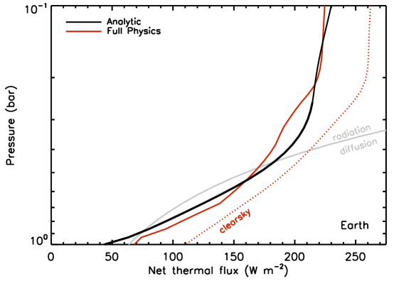
Figure 1: Comparison between the analytic expression for net thermal radiative flux (black; Equation 21) and the net thermal radiative flux computed from a full physics radiative transfer model (red). For the full physics model, weighted partially-cloudy (solid) and clearsky (dotted) cases are shown. For the analytic treatment, the thickened portion of the curve indicates the convective portion of the atmosphere. Also shown is the net thermal radiative flux computed in the radiative diffusion limit (grey; Equation 23).

A comparison between the net thermal radiative fluxes computed by the full physics model versus our analytic treatment is shown in Figure 1. For the full physics model, we include both the weighted partially cloudy scenario as well as a clearsky calculation. Also shown is a net thermal radiative flux profile in the radiation diffusion limit (Equation 23). Our analytic treatment reproduces both the shape and magnitude of the full physics partially cloudy model, whereas the shape of the radiation diffusion expression is a poor match. This latter finding simply stems from the grey Earth model not being particularly opaque to thermal radiation, with $\tau_{0}=2.8$.

3.2 Venus

To compare against Venus, we adopt thermal structure and radiative flux profiles from a new one-dimensional full physics radiative-convective model (Robinson and Crisp, 2018). Critically, this model has been shown to reproduce Venus’ observed thermal structure (Tellmann et al., 2009) as well as the Venus International Reference Atmosphere model (Moroz and Zasova, 1997). Additionally, this full physics tool reproduces probe-derived observations of the net thermal (Revercomb et al., 1985) and solar (Tomasko et al., 1980) radiative flux profiles in Venus’ atmosphere.

Robinson and Catling (2012) proposed that the $\tau$-$p$ relationship in the deep atmosphere of Venus is likely to be less steep than $n=2$ due to strong overlap of absorption lines. Indeed, here we find that adopting $n=2$ yields a surface net thermal flux that is over an order of magnitude smaller than the value from our full physics model. Thus, we explore a model with $n=1$.

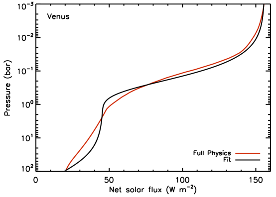
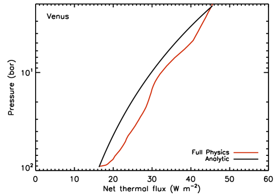
Figure 2: Top panel shows our parameterized fit (black) to the full physics net solar flux profile (red) for Venus using Equation 26. Bottom panel is the same as Figure 1 but for Venus, highlighting the atmosphere below the Cytherean clouds. The radiation diffusion limit is omitted as strongly opaque atmospheric conditions imply our analytic expression (Equation 21) completely overlaps this limit.

The net solar flux profile beneath the Cytherean clouds is only a weak function of pressure, decreasing by only about 50% over two orders of magnitude in pressure. While this profile is not well reproduced by an exponential function, Figure 2 shows a reasonable reproduction of the net solar flux profile using Equation 26. This reproduction adopts $F^{\odot}_{1}=110$ W m^-2, $F^{\odot}_{2}=50$ W m^-2, $k_{1}=0.5$, and $k_{2}=9\times 10^{-4}$. With our parameterized net solar flux profile and setting $p_{0}=92.1$ bar, $\gamma=1.3$, $\alpha=0.8$, and $T_{0}=730$ K, we find $\tau_{\rm{rc}}=20$ and $\tau_{0}=900$.

We compare our analytic models of the net thermal radiative flux to that computed by the full physics model in Figure 2. The radiation diffusion limit is not shown as the large thermal grey optical depths cause Equation 21 to completely overlap the radiation diffusion expression. Critically, our analytic model reproduces the shape of the full physics simulation, further justifying our choice of $n=1$. Additionally, the analytic model reproduces the magnitude of the net thermal flux throughout the deep atmosphere below the Venusian clouds.

3.3 Cloudfree Jupiter

Finally, to explore a scenario with a diffuse lower boundary, we compare Equation 21 to results from a widely-used one-dimensional climate model for gaseous Solar System planets and exoplanets (Marley et al., 1999; Fortney et al., 2008). For this spectrally-resolved climate model, we adopt appropriate modern Jupiter parameters from Fortney et al. (2011). We omit clouds from our model runs for two key reasons. First, and as discussed in Fortney et al. (2011), modeled clouds lack a treatment for the absorptive chromophores in Jupiter’s aerosols, thereby creating a simulated world with an unphysically large Bond albedo. Second, implementing clouds within this full physics model introduces a large number of free parameters, many of which are poorly constrained. As our primary goal is just to compare a simple analytic treatment with a more sophisticated numerical treatment of climate and radiation, we argue that clouds introduce unnecessary complexities.

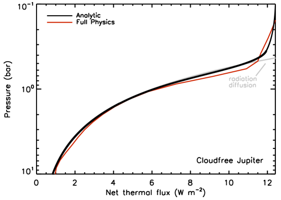
Figure 3: Same as Figure 1 but for a cloudfree Jupiter.

The convective portion of the cloudfree Jupiter atmosphere (where Equation 21 applies) is likely to be in the regime where pressure-broadening and pressure-induced absorption (especially due to H₂-H₂ and H₂-He pairs) will dominate the opacity, implying $n=2$ is appropriate. Adopting this value of $n$, the net solar radiative flux profile from our cloudfree Jupiter climate simulation is well reproduced with Equation 26, yielding $F^{\odot}_{1}=3.4$ W m^-2, $F^{\odot}_{2}=3.6$ W m^-2, $k_{1}=0.28$, and $k_{2}=2.3\times 10^{-3}$. Using these within the context of the Robinson and Catling (2012) model — adopting $p_{0}=1.1$ bar, $\gamma=1.4$, $\alpha=1$, and $T_{0}=160$ K, all taken from the equilibrium climate solution from the full physics model — yields $\tau_{0}=5.3$ and $\tau_{\rm{rc}}=0.58$. A comparison between the net thermal radiative fluxes from our analytic model versus the full physics model are shown in Figure 3. The analytic model follows the radiation diffusion limit below about $0.5$ bar (where $D\tau$ is roughly 2), and the result from Equation 21 is an excellent reproduction of the full physics model in both the convective portion of the atmosphere and the lower (radiative) portion of the stratosphere.

4 Model Behavior

Intuition for the shape of the profiles for the upwelling, downwelling, and net thermal radiative fluxes can be obtained by manipulating Equations 16, 19, and 21, and by exploring the resulting expressions for a range of physically-motivated values. Inspecting Equations 16 and 19, for $\tau_{\rm{rc}}\ll\tau\ll\tau_{0}$ we have,

$$F^{+}\left(\tau\right)\approx\frac{\sigma T_{0}^{4}}{\left(D\tau_{0}\right)^{4\beta/n}}\Gamma\left(1+4\beta/n,D\tau\right)e^{D\tau},$$ (27)

$$F^{-}\left(\tau\right)\approx\frac{\sigma T_{0}^{4}}{\left(D\tau_{0}\right)^{4\beta/n}}\mathinner{\!\left\lvert\Gamma\left(1+4\beta/n,-D\tau\right)\right\rvert}e^{-D\tau},$$ (28)

indicating that curves of the form $\Gamma\left(1+4\beta/n,D\tau\right)e^{D\tau}$ for the upwelling case, and $\mathinner{\!\left\lvert\Gamma\left(1+4\beta/n,-D\tau\right)\right\rvert}e^{-D\tau}$ for the downwelling case, help indicate the shape of the thermal radiative flux profiles. We refer to such functions as the “modified” upwelling or downwelling flux, and plot several such pairs of curves in Figure 4 for a range of physically-motivated values of $4\beta/n$. Recall that $\beta/n$ indicates the steepness of the $T$-$\tau$ relationship, so that $4\beta/n$ controls the gradient in the Stefan-Boltzmann emittance.

Regarding the net thermal radiative flux given in Equation 21, we can add $F^{-}\left(\tau_{\rm{rc}}\right)e^{-D\left(\tau-\tau_{\rm{rc}}\right)}$ from both sides and divide by $\sigma T_{0}^{4}$ to yield a “modified” net thermal radiative flux of the form,

$$\begin{split}\frac{F_{\rm{net}}\left(\tau\right)+F^{-}(\tau_{\rm{rc}})e^{-D\left(\tau-\tau_{\rm{rc}}\right)}}{\sigma T_{0}^{4}}=~{}~{}~{}~{}~{}~{}~{}~{}~{}~{}~{}~{}~{}~{}~{}\\ ~{}(1+f)e^{-D(\tau_{0}-\tau)}~{}~{}+\\ ~{}\left(D\tau_{0}\right)^{-4\beta/n}\Big{[}\Gamma\left(1+4\beta/n,D\tau\right)e^{D\tau}-\Gamma\left(1+4\beta/n,D\tau_{0}\right)e^{D\tau}~{}~{}-\\ \mathinner{\!\left\lvert\Gamma\left(1+4\beta/n,-D\tau\right)e^{-D\tau}-\Gamma\left(1+4\beta/n,-D\tau_{\rm{rc}}\right)e^{-D\tau}\right\rvert}\Big{]}\ .\end{split}$$ (29)

Thus, the function on the right-hand side of this expression (which depends only on $4\beta/n$, $\tau_{0}$, $\tau_{\rm{rc}}$, and $\tau$) indicates the shape of the net thermal radiative flux profile. Furthermore, this function will approach the true shape of the net thermal radiative flux profile for large $D\left(\tau-\tau_{\rm{rc}}\right)$, as the upper boundary condition flux term, $F^{-}\left(\tau_{\rm{rc}}\right)e^{-D\left(\tau-\tau_{\rm{rc}}\right)}$, is exponentially attenuated away from the radiative-convective boundary.

To understand the overall behavior of the net thermal radiative flux profile, we plot the function with nominal values ($\tau_{0}=5$, $\tau_{\rm{rc}}=.5$, and $4\beta/n=.45$) and compare them to profiles where a single parameter is varied. We consider scenarios with either a solid or diffuse lower boundary condition. Typically, scenarios with different lower boundary conditions only diverge from one another when $\tau$ approaches $\tau_{0}$.

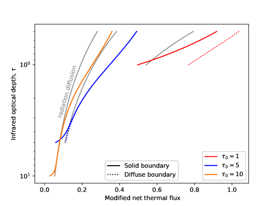
Figure 5: Comparison of the modified net thermal flux (Equation 29) with varying values of $\tau_{0}$ and fixed $\tau_{\rm{rc}}=0.45$ and $4\beta/n=0.45$. Each value is explored using both the solid boundary and the diffuse boundary. Each profile is plotted from $\tau_{\rm{rc}}$ to their respective value of $\tau_{0}$. The x-axis represents our modified net thermal flux on a linear scale while the y-axis shows the infrared optical depth on a logarithmic scale.

Modified net radiative flux profiles for cases where $\tau_{0}$ is varied to either $\tau_{0}=1$ or $\tau_{0}=10$ are shown in Figure 5. As the radiation diffusion limit is dependent on $\tau_{0}$, each profile also has a unique limit, that (for $\tau_{0}=5$ and $\tau_{0}=10$) meets with the modified net flux for the diffuse boundary at large values of $\tau$. The case where $\tau_{0}=1$ is not opaque enough for the atmosphere to reach the radiation diffusion limit. Furthermore, while the two larger values of $\tau_{0}$ have solid and diffuse profiles that match at small values of $\tau$, for $\tau_{0}=1$, the atmosphere is transparent enough that the lower boundary condition affects the entire modified net thermal flux profile.

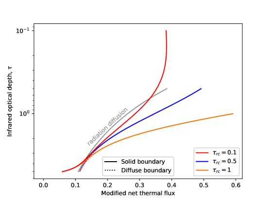
Figure 6: Same as Figure 5, except varying $\tau_{\rm{rc}}$. We fix $\tau_{0}=5$ and $4\beta/n=0.45$.

After returning to our nominal value of $\tau_{0}=5$, we modify $\tau_{\rm{rc}}$ from $\tau_{\rm{rc}}=0.5$ to values of $\tau_{\rm{rc}}=0.1$ and $\tau_{\rm{rc}}=1$, the profiles of which are seen in Figure 6. In this case, all values of $\tau_{\rm{rc}}$ share the same radiative diffusion limit as it is not dependent on $\tau_{\rm{rc}}$. We see that the modified net thermal flux curve for $\tau_{\rm{rc}}=0.1$ tends towards a constant value at low optical depths. This behavior stems from (1) our removing the downwelling thermal flux boundary condition in the modified net flux expression, and (2) the general inability of low-opacity regions of the atmosphere to strongly emit or absorb radiative flux. Finally note that, as $\tau$ approaches $\tau_{0}$, the modified net flux curves converge. This demonstrates that the dependence on $\tau_{\rm{rc}}$ is lost at large optical depths, which is expected as thermal fluxes are not sensitive to the radiative-convective boundary when this boundary is separated by many optical depths.

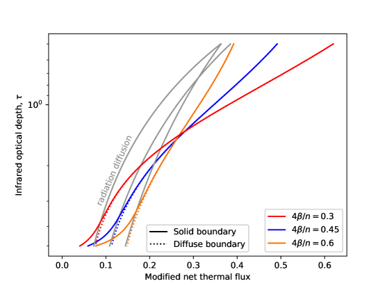
Figure 7: Same as Figure 5, except varying $4\beta/n$. We fix $\tau_{0}=5$ and $\tau_{\rm{rc}}=0.5$.

Lastly, we explore variations in $4\beta/n$ in Figure 7. We vary our nominal value ($4\beta/n=0.45$) to $4\beta/n=0.3$ and $4\beta/n=0.6$, which are motivated by values seen in the tropospheres of Solar System worlds. As mentioned earlier, $4\beta/n$ controls the gradient in the Stefan-Boltzmann emittance in the convective portion of the atmosphere, and incorporates a modified dry adiabat (adjusted due to, e.g., latent heat release from condensation). As can be seen in Figure 7, modified net thermal radiative flux models with different values of $4\beta/n$ approach their respective radiation diffusion limits at depth, and have distinct slopes (stemming from the different $T$-$\tau$ relationships) throughout the atmosphere.

5 Comparative Planetology

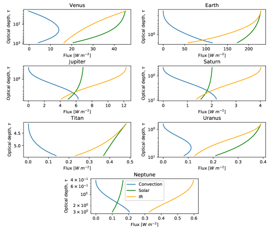
Figure 8: Net solar, thermal, and convective fluxes in Solar System planetary atmospheres from our analytic treatment and adopting model parameters from Table 1. For all plots, the convective flux is shown in blue, the net solar flux is shown in green, and the net infrared flux is shown in orange. All profiles are plotted for each world over their respective $\tau_{\rm{rc}}$–$\tau_{0}$ range, with the y-axis indicating $\tau$ (i.e., the grey thermal optical depth) on a log scale, with the exception of Titan which is plotted on a linear scale.

We can use our analytic treatments to explore energy balances for a variety of worlds across the Solar System. To accomplish this, we use Equation 26 to determine the net solar radiative flux, Equation 21 to compute the net thermal radiative flux, and Equation 22 to find the convective heat flux. Requisite model input parameters are taken from Table 1 of Robinson and Catling (2014), which were designed to reproduce the planetary average thermal structures of key Solar System worlds with thick atmospheres. These parameters, as well as our parameters for Venus derived in Section 3, are given in Table 1. In our analysis, we include Venus, Earth, Jupiter, Saturn, Titan, Uranus, and Neptune. These profiles of energy flux versus thermal optical depth are shown in Figure 8. We emphasize each world’s troposphere, highlighting the respective region between $\tau_{\rm{rc}}$–$\tau_{0}$ for each planet.

In our models and over the range of optical depths we investigate, Earth has the largest convective heat flux compared to any other world in our investigation. These large convective heat fluxes for Earth result from (1) our planet’s close proximity to the Sun paired with a moderately low albedo, leading to large amounts of absorbed solar radiation, and (2) Earth’s relatively high atmospheric transparency to shortwave radiation, which implies that a significant amount of the absorbed solar radiation is deposited at the surface where thermal radiative transport is impeded by larger atmospheric thermal opacities. The role that this transparency plays can be seen in particular when comparing the convective heat flux profiles of Earth and Venus. As Venus has a thick, cloudy atmosphere, relatively little solar radiation is reaches the surface and deep atmosphere, resulting in a weakly convective atmosphere despite being closer to the Sun.

Flux profiles for Jupiter and Saturn show overall similar shapes. Notice here that the net thermal radiative flux does not equal the net solar flux at the radiative-convective boundary, where the difference between these two quantities is simply the internal heat flux for each respective world. Near the bottom of the depicted profiles, the net solar flux is rapidly being attenuated and the net thermal radiative flux is approaching the radiation diffusion limit. Thus, at slightly larger optical depths than those shown here, the convective flux will simply approach the difference between the internal heat flux and the power-law radiation diffusion limit for the net thermal radiative flux. Neptune shows similar behaviors to Jupiter and Saturn, except that the net thermal radiative flux is driven to relatively large values near (and above) the radiative-convective boundary by an internal heat flux that is roughly 60% larger than the total absorbed solar flux.

Both Titan and Uranus demonstrate rather unique convective heat flux profiles. For the former, and like Venus, overall weak convective fluxes are attributed to Titan’s dense, opaque methane- and haze-rich atmosphere which absorbs a large amount of the incoming solar flux in the stratosphere, preventing solar energy from reaching the deep atmosphere and surface to drive convection. In the case of Uranus, a turn-over in the convective heat flux is caused by differences in the shapes of the net solar versus net thermal fluxes (i.e., exponential drop-off versus power-law) and the near-zero internal heat flux (Pearl et al., 1990).

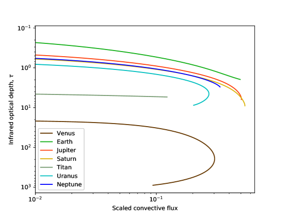
Figure 9: Scaled convective flux profiles for Solar System worlds, obtained by dividing the model-derived convective flux profile by the input deep atmosphere energy flux budget (i.e., $F_{2}^{\odot}+F_{\rm{i}}$). Here, both the x-axis and y-axis are on a logarithmic scale.

We can gain a greater intuition for similarities between convective profiles for Solar System worlds by scaling these profiles by the total tropospheric energy flux budget that must be carried by both convection and thermal radiative transport, $F^{\odot}_{2}+F_{\rm{i}}$. As in Robinson and Catling (2014), $F^{\odot}_{2}$ is the net solar flux absorbed in the deep atmosphere and at the surface (if applicable). Thus, $F_{\rm{c}}\left(\tau\right)$ scaled by $F^{\odot}_{2}+F_{\rm{i}}$ represents the fraction of the total deep atmosphere energy budget carried by convection. These scaled profiles are shown in Figure 9. Aside from Titan and Venus (discussed below), the scaled convective flux profiles show an overall similar shape, where the convective flux begins to carry a significant portion (i.e., larger than 10%) of the deep atmosphere energy budget when $D\tau$ reaches 0.7–2, which, intuitively, is where thermal radiative transport becomes inefficient due to increasingly opaque atmospheric conditions.

Regarding Titan and Venus, both have “deep” convective zones in the terminology of Sagan (1969), where “deep” convective zones have $D\tau_{\rm{rc}}$ larger than unity and “shallow” convective zones have $D\tau_{\rm{rc}}$ smaller than unity. As discussed in Robinson and Catling (2012) (their Section 3.2), the division between “deep” and “shallow” convective zones is largely controlled by $\beta/n$ and the shortwave attenuation parameter(s), $k$. The former parameter determines the critical lapse rate (in $T$-$\tau$ space) for the onset of convection. For smaller stellar attenuation parameter(s), solar flux is deposited rapidly in the deep atmosphere or at the surface, leading to convective instability. However, for larger stellar attenuation parameters (as in the case of Titan and Venus), the temperature profile is stabilized against convection by the absorption aloft of solar energy.

6 Discussion

Simple models of planetary thermal radiative transport and/or climate are only useful for understanding physical processes if such tools can be shown to reproduce observations or results from more-complex models. Critically, our grey analytic expression of the net thermal radiative flux in a planetary atmosphere, Equation 21, provides strong reproductions of results from sophisticated spectrally-resolved models, as shown in Section 3. For Venus, our comparisons indicate that the deep atmosphere likely follows a $\tau\propto p$ relationship. Also, our comparison to a cloudfree Jupiter shows that the grey assumption is an excellent approximation in the deep atmosphere, likely owing to the leading role played by H₂-H₂ and H₂-He pressure-induced absorption. Thus, grey assumptions are likely to hold in the H₂- and He-rich deep atmospheres of gas giant exoplanets.

Our Earth comparison indicates that a $\tau\propto p^{2}$ relationship yields a good reproduction of the net thermal radiative flux profile computed by a line-by-line model. Other authors have used the small scale height for water vapor in Earth’s troposphere to argue for a steeper relationship between optical depth and pressure, with $\tau\propto p^{4}$ (Weaver and Ramanathan, 1995; Frierson et al., 2006). While it is certainly true that water is the dominant thermal opacity source in the deep atmosphere of Earth, it might be that cooler temperatures 1–2 pressure scale heights above Earth’s surface shift the peak of the Planck function closer to the 15 $\mu$m CO₂ band, whose uniform mixing ratio through the atmosphere helps maintain $\tau\propto p^{2}$ in the deep atmosphere.

The uniform application of our analytic models to all Solar System worlds with thick atmospheres in Section 5 enables exploration of commonalities (and differences) in convective flux profiles. Owing to relatively strong shortwave attenuation, both Venus and Titan have “shallow” convective zones. All other worlds — Earth, Jupiter, Saturn, Uranus, and Neptune — have “deep” convective zones. These latter worlds also demonstrate a similar shape in their convective flux profiles (Figure 9), once scaled by the deep atmosphere input energy budget (i.e., $F_{2}^{\odot}+F_{\rm{i}}$). These scaled profiles show that convective transport rapidly increases when the grey thermal optical depth of the atmosphere reaches (roughly) unity. Other authors have explored convective fluxes using grey thermal radiative transport principles, and we compare our approach to these previous studies in greater detail below.

6.1 Ozawa and Ohmura

Ozawa and Ohmura (1997) adopted a grey thermal radiative transport model to explore the concept of “maximum entropy production,” wherein the steady-state radiative and convective energy fluxes are assumed to maximize the rate of entropy production. In their work, Ozawa and Ohmura (1997) varied the convective energy flux until entropy production was maximized, and thermal structures were derived from combining grey radiative transfer with an energy balance constraint (i.e., Equation 22). This approach does not require specification of a dry adiabatic lapse rate, and results in temperature profiles that are less-steep than their pure-radiative counterparts. Investigated cases all included an Earth-like net solar flux profile and total grey thermal optical depths (i.e., $\tau_{0}$) of between 1–5.

As is evident from Figure 2 in Ozawa and Ohmura (1997), equilibrium solutions for different values of $\tau_{0}$ are found to have distinct, non-constant $d\ln T/d\ln\tau$ values in the convective portion of an atmosphere, whereas this gradient is fixed as a constant ($\beta/n$) in our approach. For Ozawa and Ohmura (1997), $d\ln T/d\ln\tau$ is typically 0.08–0.1 beneath $\tau\sim 1$, falling to $<0.05$ in the less opaque regions of the atmosphere. By comparison, our simulations (which assume an adiabatic, power-law temperature-pressure relationship) have $d\ln T/d\ln\tau$ equal to 0.17, 0.09, and 0.04 for $n$ equal to 1, 2, and 4, respectively. Thus, our preferred Earth model (with $n=2$) has a markedly steeper $T-\tau$ relationship in the convective portion of the atmosphere than do solutions from Ozawa and Ohmura (1997).

Nevertheless, we can mimic solutions to equilibrium thermal structures in Ozawa and Ohmura (1997) using the Robinson and Catling (2012) model. Instead of the typical approach, where equilibrium thermal structures are determined using energy balance and thermal structure continuity constraints to solve for $\tau_{\rm{rc}}$ and $\tau_{0}$ once $T_{0}$ (the surface temperature) and $\beta/n$ are specified, we can specify $T_{0}$ and $\tau_{0}$ (both from Table 1 in Ozawa and Ohmura, 1997) and find the values of $\tau_{\rm{rc}}$ and $\beta/n$ that yield an equilibrium thermal structure. These models all have very “shallow” convective zones, with $\tau_{\rm{rc}}<0.1$ for $\tau_{0}$ ranging between 1–5, whereas the Earth model given in Robinson and Catling (2014) has $\tau_{\rm{rc}}=0.15$ and $\tau_{0}=2$. Our models with fitted $T$-$\tau$ relationships also have smaller $d\ln T/d\ln\tau$, indicating less steep thermal structures. This results in larger downwelling thermal radiative fluxes at the surface in our simulations, and, thus, larger convective convective fluxes at the planetary surface.

For a specific point of comparison, we investigate the Ozawa and Ohmura (1997) case with $\tau_{0}=3$ and $T_{0}=289$, as this most closely matches Earth’s mean surface temperature. This particular case has a downwelling thermal radiative flux at the surface of 337 W m^-2 and a convective flux at the surface of 89 W m^-2 (see Table 1 in Ozawa and Ohmura, 1997). By comparison, when we adopt a model that fits for $\tau_{\rm{rc}}$ and $\beta/n$ while using the same values of $\tau_{0}$ and $T_{0}$, we find a downwelling thermal radiative flux at the surface of 370 W m^-2 and a surface convective heat flux of 120 W m^-2. Estimates of Earth’s surface energy budget typically find a downwelling thermal radiative flux at the surface of roughly 330–340 W m^-2 and a surface convective heat flux (in both dry and moist processes) of 100–110 W m^-2 (Trenberth et al., 2009; Loeb et al., 2009). Thus our “fitted $\beta/n$” approach overestimates the downwelling thermal radiative flux at the surface by about 10%, resulting in a similar overestimate in the convective heat flux.

Our more realistic Earth model (adopted in Section 5) has 330 W m^-2 of downwelling thermal radiative flux and 110 W m^-2 of convective heat flux at the surface, which are quite close to the global average estimates and comparable to the Ozawa and Ohmura (1997) case. A key difference is that our adopted $d\ln T/d\ln\tau$ is motivated by the physics of (modified) dry adiabats and pressure-broadened opacities rather than maximizing the rate of entropy production. Energy flux agreements between our approach and the maximum entropy generation technique indicate that our analytic models could be used to explore physical underpinnings in maximum entropy generation models.

6.2 Lorenz and McKay

Lorenz and McKay (2003) used expressions for grey thermal radiative equilibrium and realistic data and models to propose an empirical expression for the convective flux at a planetary surface of the form,

$$F_{\rm{c}}=F_{\rm{net}}^{\odot}\left(\tau_{0}\right)\frac{\tau_{0}}{C+D\tau_{0}}\ ,$$ (30)

where $C$ and $D$ are free parameters (the latter is distinct from the diffusivity factor used above). Typical values for both $C$ and $D$ were in the range 1–2. Convective fluxes in giant planets is only briefly discussed by Lorenz and McKay (2003), who note that the deep atmospheres of gas giants will have large $\tau_{0}$ and $F_{\rm{c}}\approx F_{\rm{i}}$, indicating that replacing $F_{\rm{net}}^{\odot}\left(\tau_{0}\right)$ with $F_{\rm{i}}$ in the empirical expression and adopting $D=1$ would fit the deep atmospheres of giants.

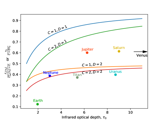
Figure 10: Variants of the heuristic convective flux expression given by Lorenz and McKay (2003) compared to the Solar System worlds explored with our analytic model.

We investigate the applicability of the empirical expression from Lorenz and McKay (2003) in Figure 10. Inclusion of the gas and ice giants is not straightforward, as these worlds lack a “surface” where the empirical expression is designed to apply. Nevertheless, as the convective flux in the tropospheres of these worlds must carry some fraction of the combined net solar and internal heat fluxes, we opt to plot $F_{\rm{c}}\left(\tau_{0}\right)/\left[F_{\rm{net}}^{\odot}\left(\tau_{0}\right)+F_{\rm{i}}\right]$ versus $\tau_{0}$ for the worlds in Section 5. For terrestrial worlds, the optical depth is referenced at the surface, while for gaseous worlds we use the 1 bar pressure level. Of course, adopting the 1 bar pressure level for gaseous worlds is arbitrary, and using other pressure levels would result in values of $F_{\rm{c}}\left(\tau_{0}\right)/\left[F_{\rm{net}}^{\odot}\left(\tau_{0}\right)+F_{\rm{i}}\right]$ that span from 0 at the radiative-convective boundary and unity at great depths. Focusing only on solid-surface planets, the shown variations of the Lorenz and McKay (2003) expression do not offer perfect fits, although the performance of this expression is surprising given its two-parameter simplicity.

7 Conclusions

Net thermal and convective energy fluxes are critically important to determining atmospheric thermal structure, especially in one-dimensional (vertical) planetary climate models. We derive a simple expression for the net downwelling thermal radiative flux in a planetary troposphere where the relationships between temperature, pressure, and optical depth are all expressed as power-laws. When combined with previous results, our new treatment yields an analytic expression for the net thermal radiative flux in a convective planetary troposphere. For appropriate, physically-based input parameters, our analytic net thermal radiative flux expression reproduces results from more-sophisticated, spectrally-resolved models applied to Earth, Venus, and a cloudfree Jupiter. Application of our model across the Solar System demonstrates common shapes and scalings in the convective flux profiles of Earth, Jupiter, Saturn, Uranus, and Neptune. Further applications of our model sheds new light on both “maximum entropy production” principles as well as other simple treatments of convection. Simple models remain an excellent tool for inter-comparing processes in planetary atmospheres both within and beyond the Solar System.

Radiative-Convective Model Parameters for Solar System Worlds World Venus Earth Jupiter Saturn Titan Uranus Neptune $p_{0}$ (bar) 92.1 1 1 1 1.5 1 1 $T_{0}$ (K) 730 288 166 135 94 76 72 $a$ 0.8 0.6 0.85 0.94 0.77 0.83 0.87 $\gamma$ 1.3 1.4 1.4 1.4 1.4 1.4 1.4 $n$ 1 2 2 2 2 2 2 $F_{1}^{\odot}$ (W m^-2) 110 7 1.3 0.41 1.49 0.24 0.09 $F_{2}^{\odot}$ (W m^-2) 46 233 7.0 2.04 1.12 0.41 0.18 $F_{\rm{i}}^{\odot}$ (W m^-2) 0 0 5.4 2.01 0 $\sim$ 0 0.43 $k_{1}$ 0.518 90 90 180 120 220 580 $k_{2}$ $9\times 10^{-4}$ 0.16 0.05 0.03 0.2 0.08 0.2 $\tau_{\rm{rc}}$ 20 0.15 0.34 0.44 4.4 0.63 0.42 $\tau_{0}$ 990 1.9 6.3 9.0 5.6 8.7 3.0

Table 1: Model parameters used in our analytic expressions. Venus parameters come from fits in Section 3. Parameters for all other worlds come from Robinson and Catling (2014) with an updated diffuse lower boundary condition for Jupiter, Saturn, Uranus, and Neptune.

Figure 4: Profiles of the “modified” upwelling (solid) and downwelling (dashed) thermal radiative flux profiles, obtained by dividing Equations 27 and 28 by $\sigma T_{0}^{4}/\left(D\tau_{0}\right)^{4\beta/n}$. Profiles are shown for a range of physically-motivated values of $4\beta/n$. Also shown are power-laws of the form $\left(D\tau\right)^{4\beta/n}$ (dashed), demonstrating that the modified upwelling and downwelling thermal radiative fluxes approach $\sigma T\left(\tau\right)^{4}$ in optically thick conditions.

References

- Andrews (2010) David G Andrews. An introduction to atmospheric physics. Cambridge University Press, 2010.
- Armstrong (1968) BH Armstrong. Theory of the diffusivity factor for atmospheric radiation. Journal of Quantitative Spectroscopy and Radiative Transfer, 8(9):1577–1599, 1968.
- Catling and Kasting (2017) D.C. Catling and J.F. Kasting. Atmospheric Evolution on Inhabited and Lifeless Worlds. Cambridge University Press, 2017. ISBN 9780521844123. URL https://books.google.com/books?id=dchoDgAAQBAJ.
- Fortney et al. (2008) J. J. Fortney, M. S. Marley, D. Saumon, and K. Lodders. Synthetic Spectra and Colors of Young Giant Planet Atmospheres: Effects of Initial Conditions and Atmospheric Metallicity. Astrophys J, 683:1104-1116, August 2008. doi: 10.1086/589942.
- Fortney et al. (2011) J. J. Fortney, M. Ikoma, N. Nettelmann, T. Guillot, and M. S. Marley. Self-consistent Model Atmospheres and the Cooling of the Solar System’s Giant Planets. Astrophys J, 729:32, March 2011.
- Frierson et al. (2006) D. M. W. Frierson, I. M. Held, and P. Zurita-Gotor. A Gray-Radiation Aquaplanet Moist GCM. Part I: Static Stability and Eddy Scale. Journal of Atmospheric Sciences, 63:2548–2566, October 2006. doi: 10.1175/JAS3753.1.
- Gierasch and Goody (1968) P. Gierasch and R. Goody. A study of the thermal and dynamical structure of the martian lower atmosphere. Planetary Space Sci, 16:615–646, May 1968.
- Gierasch and Conrath (1985) P. J. Gierasch and B. J. Conrath. Energy conversion processes in the outer planets. In G. E. Hunt, editor, Recent Advances in Planetary Meteorology, pages 121–146. Cambridge Univ. Press, Cambridge, 1985.
- Goody et al. (1989) Richard Goody, Robert West, Luke Chen, and David Crisp. The correlated-k method for radiation calculations in nonhomogeneous atmospheres. Journal of Quantitative Spectroscopy and Radiative Transfer, 42(6):539–550, December 1989. doi: 10.1016/0022-4073(89)90044-7.
- Guillot (2010) T. Guillot. On the radiative equilibrium of irradiated planetary atmospheres. Astron Astrophys, 520:A27, September 2010. doi: 10.1051/0004-6361/200913396.
- Hansen (2008) B. M. S. Hansen. On the Absorption and Redistribution of Energy in Irradiated Planets. Astrophys J Supp, 179:484–508, December 2008. doi: 10.1086/591964.
- Hart (1978) M. H. Hart. The evolution of the atmosphere of the earth. Icarus, 33:23–39, January 1978.
- Heng et al. (2012) K. Heng, W. Hayek, F. Pont, and D. K. Sing. On the effects of clouds and hazes in the atmospheres of hot Jupiters: semi-analytical temperature-pressure profiles. Mon Not Royal Astro Soc, 420:20–36, February 2012. doi: 10.1111/j.1365-2966.2011.19943.x.
- Heng et al. (2014) K. Heng, J. M. Mendonça, and J.-M. Lee. Analytical Models of Exoplanetary Atmospheres. II. Radiative Transfer via the Two-stream Approximation. Astrophys J Supp, 215:4, November 2014. doi: 10.1088/0067-0049/215/1/4.
- Herbert et al. (2013) C. Herbert, D. Paillard, and B. Dubrulle. Vertical Temperature Profiles at Maximum Entropy Production with a Net Exchange Radiative Formulation*. Journal of Climate, 26:8545–8555, November 2013. doi: 10.1175/JCLI-D-13-00060.1.
- Hubeny et al. (2003) I. Hubeny, A. Burrows, and D. Sudarsky. A Possible Bifurcation in Atmospheres of Strongly Irradiated Stars and Planets. Astrophys J, 594:1011–1018, September 2003. doi: 10.1086/377080.
- Lacis and Oinas (1991) A. A. Lacis and V. Oinas. A description of the correlated-k distribution method for modelling nongray gaseous absorption, thermal emission, and multiple scattering in vertically inhomogeneous atmospheres. J Geophys Res, 96:9027–9064, May 1991. doi: 10.1029/90JD01945.
- Loeb et al. (2009) N. G. Loeb, B. A. Wielicki, D. R. Doelling, G. L. Smith, D. F. Keyes, S. Kato, N. Manalo-Smith, and T. Wong. Toward Optimal Closure of the Earth’s Top-of-Atmosphere Radiation Budget. Journal of Climate, 22:748, 2009. doi: 10.1175/2008JCLI2637.1.
- Lorenz and McKay (2003) R. D. Lorenz and C. P. McKay. A simple expression for vertical convective fluxes in planetary atmospheres. Icarus, 165:407–413, October 2003. doi: 10.1016/S0019-1035(03)00205-7.
- Madhusudhan and Seager (2009) N. Madhusudhan and S. Seager. A Temperature and Abundance Retrieval Method for Exoplanet Atmospheres. Astrophys J, 707:24–39, December 2009.
- Manabe and Strickler (1964) S. Manabe and R. F. Strickler. Thermal Equilibrium of the Atmosphere with a Convective Adjustment. Journal of Atmospheric Sciences, 21:361–385, July 1964.
- Marley and Robinson (2014) M. S. Marley and T. D. Robinson. On the Cool Side: Modeling the Atmospheres of Brown Dwarfs and Giant Planets. Annual Review of Astronomy and Astrophysics, in review:279–323, August 2014. doi: 10.1146/annurev-astro-082214-122522.
- Marley et al. (1999) M. S. Marley, C. Gelino, D. Stephens, J. I. Lunine, and R. Freedman. Reflected Spectra and Albedos of Extrasolar Giant Planets. I. Clear and Cloudy Atmospheres. Astrophys J, 513:879–893, March 1999.
- McClatchey et al. (1972) R. A. McClatchey, R. W. Fenn, J. E. A. Selby, F. E. Volz, and J. S. Garing. Optical Properties of the Atmosphere (Third Edition). Technical report, Air Force Cambridge Research Labs, August 1972.
- McKay et al. (1999) C. P. McKay, R. D. Lorenz, and J. I. Lunine. Analytic Solutions for the Antigreenhouse Effect: Titan and the Early Earth. Icarus, 137:56–61, January 1999.
- Meadows and Crisp (1996) V. S. Meadows and D. Crisp. Ground-based near-infrared observations of the Venus nightside: The thermal structure and water abundance near the surface. J Geophys Res, 101:4595–4622, 1996.
- Mellor and Yamada (1974) G. L. Mellor and T. Yamada. A Hierarchy of Turbulence Closure Models for Planetary Boundary Layers. Journal of Atmospheric Sciences, 31:1791–1806, October 1974. doi: 10.1175/1520-0469(1974)031¡1791:AHOTCM¿2.0.CO;2.
- Mitchell et al. (2006) J. L. Mitchell, R. T. Pierrehumbert, D. M. W. Frierson, and R. Caballero. The dynamics behind Titan’s methane clouds. Proceedings of the National Academy of Science, 103:18421–18426, November 2006. doi: 10.1073/pnas.0605074103.
- Mohandas et al. (2018) G. Mohandas, M. E. Pessah, and K. Heng. Analytical Models of Exoplanetary Atmospheres. V. Non-gray Thermal Structure with Coherent Scattering. Astrophys J, 858:1, May 2018. doi: 10.3847/1538-4357/aab35d.
- Moroz and Zasova (1997) VI Moroz and LV Zasova. Vira-2: A review of inputs for updating the venus international reference atmosphere. Advances in Space Research, 19(8):1191–1201, 1997.
- Nakajima et al. (1992) S. Nakajima, Y.-Y. Hayashi, and Y. Abe. A study on the ’runaway greenhouse effect’ with a one-dimensional radiative-convective equilibrium model. Journal of Atmospheric Sciences, 49:2256–2266, December 1992. doi: 10.1175/1520-0469(1992)049¡2256:ASOTGE¿2.0.CO;2.
- Ozawa and Ohmura (1997) H. Ozawa and A. Ohmura. Thermodynamics of a Global-Mean State of the Atmosphere–A State of Maximum Entropy Increase. Journal of Climate, 10:441–445, March 1997. doi: 10.1175/1520-0442(1997)010¡0441:TOAGMS¿2.0.CO;2.
- Parmentier and Guillot (2014) V. Parmentier and T. Guillot. A non-grey analytical model for irradiated atmospheres. I. Derivation. Astron Astrophys, 562:A133, February 2014. doi: 10.1051/0004-6361/201322342.
- Parmentier et al. (2015) V. Parmentier, T. Guillot, J. J. Fortney, and M. S. Marley. A non-grey analytical model for irradiated atmospheres. II. Analytical vs. numerical solutions. Astron Astrophys, 574:A35, February 2015. doi: 10.1051/0004-6361/201323127.
- Pearl et al. (1990) J. C. Pearl, B. J. Conrath, R. A. Hanel, J. A. Pirraglia, and A. Coustenis. The albedo, effective temperature, and energy balance of Uranus, as determined from Voyager IRIS data. Icarus, 84:12–28, March 1990. doi: 10.1016/0019-1035(90)90155-3.
- Pelkowski et al. (2008) J. Pelkowski, L. Chevallier, B. Rutily, and O. Titaud. Exact results in modeling planetary atmospheres III: The general theory applied to the Earth’s semi-gray atmosphere. J Quant Spec Rad Trans, 109:43–51, January 2008. doi: 10.1016/j.jqsrt.2007.07.014.
- Pierrehumbert (2011) R.T. Pierrehumbert. Principles of planetary climate. Cambridge Univ Pr, 2011.
- Pollack (1969) J. B. Pollack. Temperature Structure of Nongray Planetary Atmospheres. Icarus, 10:301–313, March 1969. doi: 10.1016/0019-1035(69)90031-1.
- Revercomb et al. (1985) HE Revercomb, LA Sromovsky, VE Suomi, and RW Boese. Net thermal radiation in the atmosphere of venus. Icarus, 61(3):521–538, 1985.
- Robinson (2015) T. D. Robinson. Completely Colorblind: Advances in Gray Techniques and Applications to Planets Near and Far. ArXiv e-prints, November 2015.