Pointing optimization for IACTs on indirect dark matter searches

Abstract

We present a procedure to optimize the offset angle (usually also known as the wobble distance) and the signal integration region for the observations and analysis of extended sources by Imaging Atmospheric Cherenkov Telescopes (IACTs) such as MAGIC, HESS, VERITAS or (in the near future), CTA. Our method takes into account the off-axis instrument performance and the emission profile of the gamma-ray source. We take as case of study indirect dark matter searches (where an a priori knowledge on the expected signal morphology can be assumed) and provide optimal pointing strategies to perform searches of dark matter on a set of dwarf spheroidal galaxies with current and future IACTs.

1 Introduction

Imaging Atmospheric Cherenkov Telescopes (IACTs) are ground based instruments capable of detecting gamma rays with energies from $\sim$50 GeV to $\sim$100 TeV. IACT’s typical fields of view (FoVs) are of the order of $\sim$1-10^∘. Observations are often performed in the so called wobble mode (Fomin et al., 1994), in which the nominal pointing of the telescope has an offset (by a certain angle $w$, called the wobble distance) w.r.t. the position of the source under observation (or, for extended sources, to its center). Signal (or ON) region is integrated inside a circular region of angular size $\theta_{\text{c}}$ around the source while background control (or OFF) region can be defined equally around a ghost region placed symmetrically w.r.t. the pointing direction (in order to have equal acceptance). Under such wobble observation mode ON and OFF regions are observed simultaneously, what makes an efficient use of the limited duty cycles of IACTs while minimizing possible systematic differences in the acceptance for ON and OFF regions (due e.g. to atmospheric changes in the on-axis observation mode).

Unlike $\theta_{\text{c}}$ that is used in the analysis, $w$ is fixed during data taking (by fixing the pointing direction w.r.t. the center of the source). The value of $w$ can be optimized if one takes into account that for large $w$, ON and OFF regions are defined close to the edge of the FoV, where the performance of the instrument decreases while for low $w$, it may not be possible to define an appropriate signal-free OFF region. These effects become critical for moderately extended sources, as the case for instance of the expected gamma-ray signal coming from Dark Matter (DM) in nearby dwarf spheroidal galaxies (dSphs) or from pulsar wind nebulae from nearby pulsars.

Here we present a procedure to optimize the wobble distance $w$ and signal integration radius $\theta_{\text{c}}$, taking into account the off-axis performance of the instrument and the expected spatial morphology of the source. As a case study, we focus on indirect DM searches and provide optimal pointing configurations for a list of dSphs to be observed for current and future IACTs. We have implemented an open-source tool so that the procedure can be applied to optimize the pointing strategy of an arbitrary IACT observing an arbitrary circular symmetric moderate extended gamma-ray source.

The rest of this paper is structured as follows: in section 2 we introduce the IACT technique and define a set of quantities that allow us to quantify their off-axis performance; in section 3 we introduce the quality factor that we use as a figure of merit for the optimization of the pointing strategy; in section 4 we briefly discuss the DM paradigm and assess its framework, and apply the method for the case of indirect DM searches to provide optimal pointing strategies on a set of dSphs observed with current or future IACTs; finally, in section 5 we briefly discuss the current status of the software and its applicability.

2 Imaging Atmospheric Cherenkov Telescopes off-axis performance

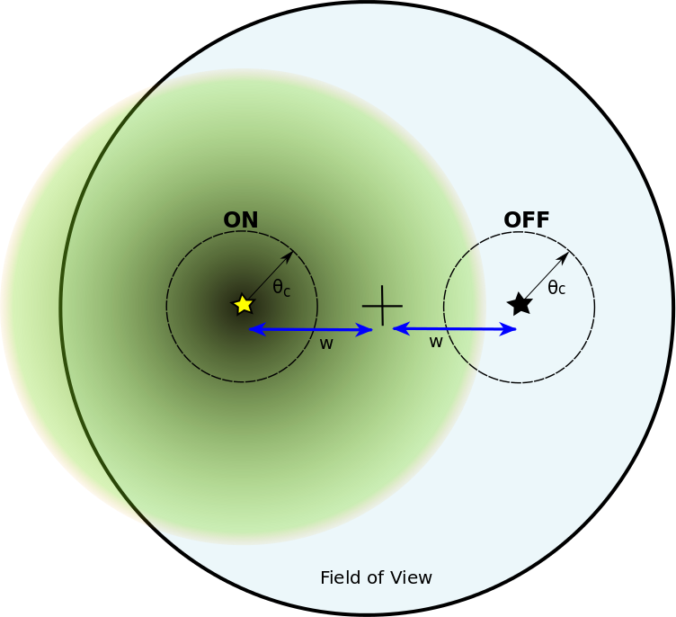
Figure 1: Schematic configuration of the FoV during wobble mode observations. The telescope pointing (black cross) has an offset distance w w.r.t. the center of the source under study (yellow star). Signal (ON) region is defined as a circle around the center of the source, with angular size $\theta_{\text{c}}$. One background control region (circular region around OFF, black star) is defined with same angular size, symmetrically w.r.t. the signal region. The leakage effect is schematically shown where, for moderately extended source (green area), signal events are also expected to be reconstructed inside OFF.

In wobble operation mode, a circular ON region of radius $\theta_{\text{c}}$ is defined centered at the source under study (observed at a distance $w$ from the center of the FoV, see Figure 1). One or several OFF regions are defined within the same FoV, in such a way that background statistical uncertainties are minimized and instrumental associated uncertainties are also kept low. For moderately extended sources, as the case we consider, typically only a single OFF region is considered in order not to overlap ON and/or OFF regions (circle ON and OFF in Figure 1).

Due to their optics and trigger strategy, IACTs have a decreasing performance for detecting gamma rays towards the edges of the FoV, w.r.t. its center (i.e. the pointing direction of the instrument). In order to characterize the off-axis performance of IACTs, we use the relative acceptance ($\epsilon$) w.r.t. the center of the FoV. This relative acceptance can be estimated as;

$$\epsilon(d)=\frac{\mathcal{R_{\text{ON}}}(d)}{\mathcal{R_{\text{ON}}}(d=0)},$$ (1)

where $\mathcal{R}_{\text{ON}}$ is the rate of events passing all the analysis cuts (i.e. gamma-ray candidates) inside the ON region, and $d$ the off-set distance w.r.t. the pointing direction (we assume $\epsilon$ to be circularly symmetric from the center of the FoV). Note that, in Equation 1, we are implicitly assuming $\theta_{\text{c}}$ to be much smaller than the scale of the FoV ($\theta_{\text{c}}\ll\sim 5^{\circ}$), otherwise, $\epsilon$ may vary from one point to another within the integration region. As it will be used later on, we could have equally written Equation 1 replacing $\mathcal{R}_{\text{ON}}$ for $\mathcal{R}_{\text{OFF}}$, with $\mathcal{R}_{\text{OFF}}$ being the rate of gamma-ray candidates inside the OFF region.

2.1 Relative acceptance for real Imaging Atmospheric Cherenkov Telescope

We compute now $\epsilon$ for the Florian Goebel Major Atmospheric Gamma-ray Imaging Cherenkov (MAGIC) telescopes and the future Cherenkov Telescope Array (CTA).

MAGIC is a system of two gamma-ray Cherenkov telescopes located at the Roque de los Muchachos Observatory in La Palma (Canary Islands, Spain), sensitive to gamma rays in the very high energy (VHE) domain, i.e. in the range between $\sim$50 GeV and $\sim$50 TeV (Aleksić et al., 2016). The MAGIC FoV is $\sim 3.5^{\circ}$ diameter. Standard point-like observations are performed in wobble mode, with $(w,\theta_{\text{c}})_{\text{MAGIC}}=(0.4^{\circ},\sim 0.1^{\circ})$. Figure 20 in Aleksić et al. (2016) shows the rate of gamma-like events detected from the direction of Crab-Nebula observed at different values of $w$, for two different stable hardware configurations of MAGIC. Using Equation 1, we compute the relative acceptance of the MAGIC telescopes ($\epsilon_{\text{MAGIC}}$) from the data from Aleksić et al. (2012) labeled as Crab Nebula post-upgrade, hereafter named MAGIC Point-like (see Figure 2).

CTA is the next generation ground-based observatory for gamma-ray astronomy at very-high energies. CTA will be the world’s largest and most sensitive high-energy gamma-ray observatory and will operate in both the northern and southern hemispheres (Acharya et al., 2017). We take CTA’s off-axis performance from https://www.cta-observatory.org/, where the relative off-axis sensitivity ($\delta$) normalized to the center of the FoV is given. In order to compute the relative acceptance of CTA ($\epsilon_{\text{CTA}}$), we need to consider that $\delta$ can be written as

$$\delta(d)= \frac{\mathcal{S}(d)}{\mathcal{S}(d=0)}\;,$$

where $\mathcal{S}$ is the sensitivity of the instrument,

i.e.: $$\mathcal{S}(d)\propto \left(\frac{N_{\text{ON}}(d)}{\sqrt{N_{\text{OFF}}(d)}}\right)^{-1}.$$ (3)

Based on subsection 2.1, Equation 1 can be re-written as:

$$\epsilon_{\text{CTA}}\left(d\right)=\frac{1}{\delta^{2}\left(d\right)}.$$ (4)

Figure 2 shows $\epsilon_{\text{CTA}}$, for the lower energy range from the northern CTA array shown in cta-observatory.org/science/cta-performance/cta-performance-archive1/ (labeled as CTA North 50-80 GeV). We assume here that $\epsilon$ for the “CTA North 50-80 GeV” is valid for the full CTA array. In reality CTA will be formed by IACTs of different kinds, with a different $\epsilon$ for each telescope type, where the method would still be valid to optimize the pointing of each telescope type individually.

We also stress that, based on $\epsilon$ in Figure 2, we cannot compare the absolute acceptances between MAGIC and CTA.

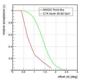
Figure 2: $\epsilon_{\text{MAGIC}}$ (red) and $\epsilon_{\text{CTA}}$ (green) as a function of $d$ recomputed from (Aleksić et al., 2016) and https://www.cta-observatory.org/ respectively.

3 Pointing optimization

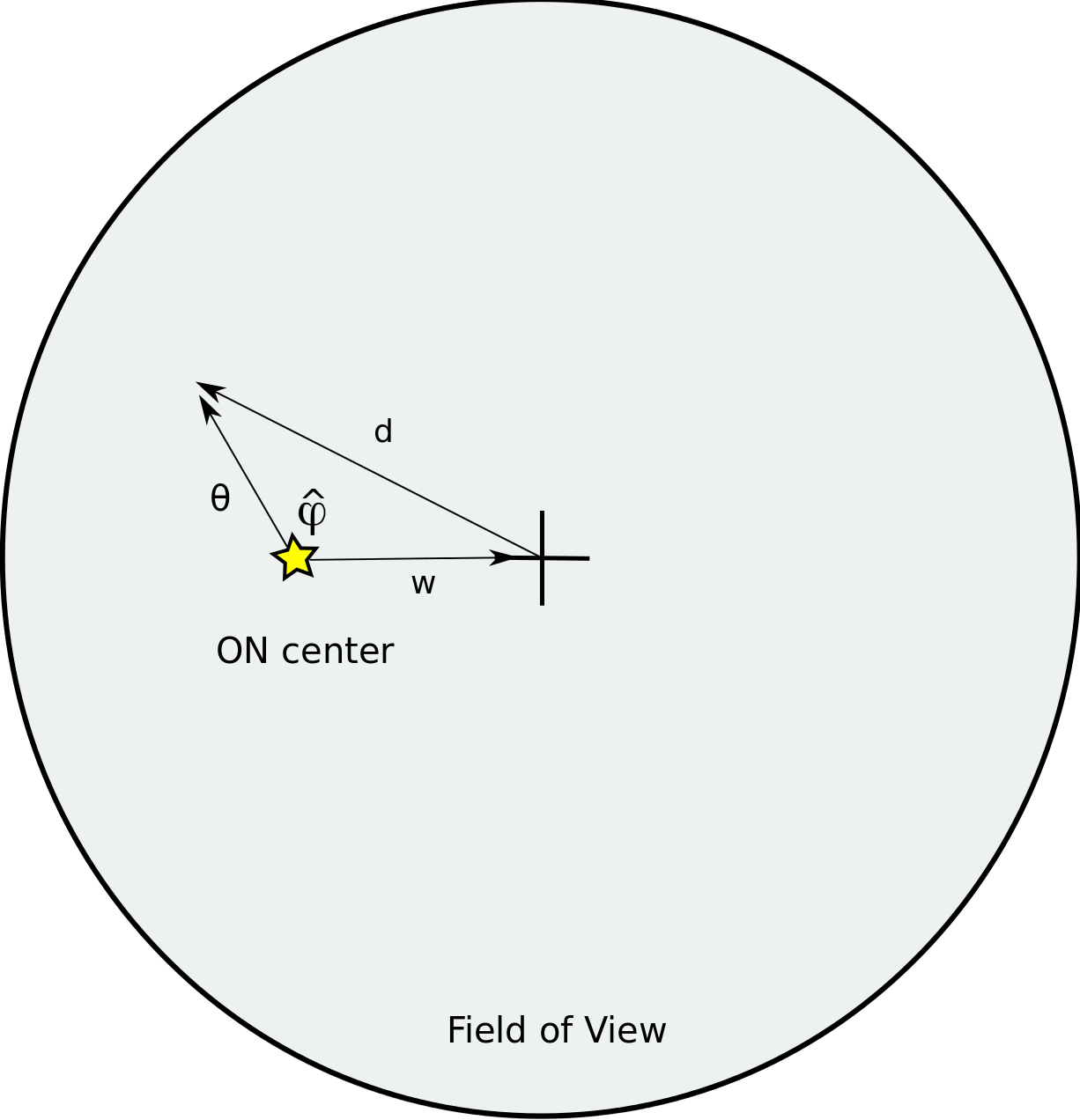
(a)

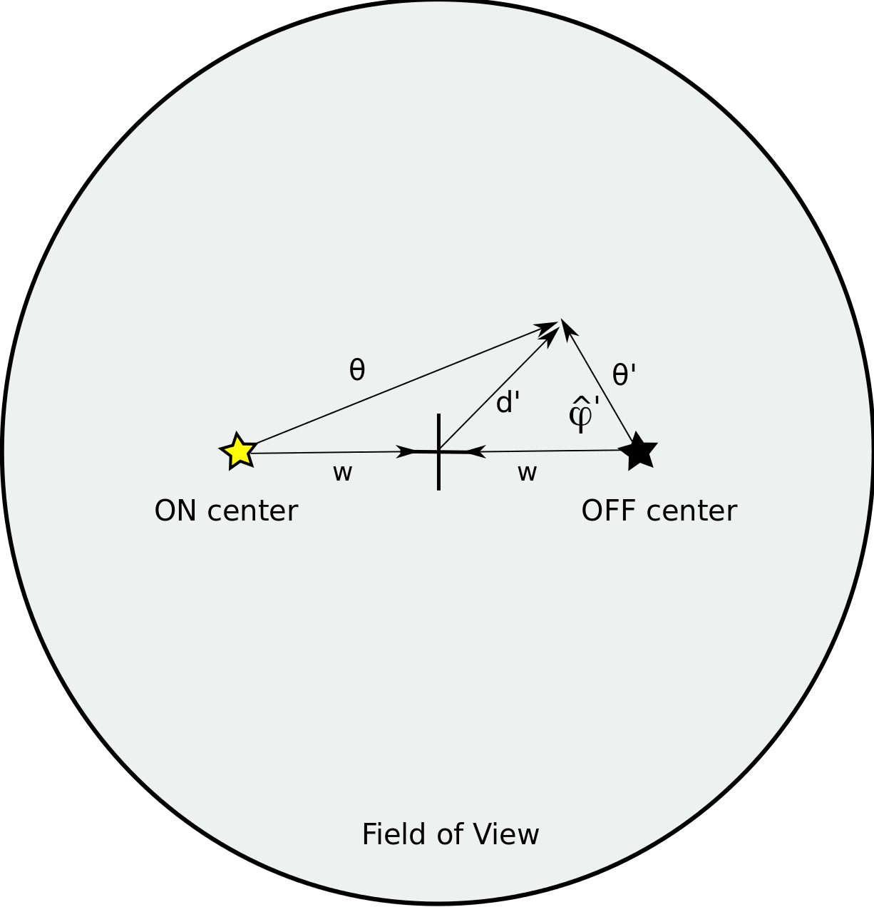
(b)

Figure 3: Definition of variables: (left) $w$ is the distance between the center of a source (yellow star) and the center of the FoV. $\theta$ is the distance between the center of the source and any point of the FoV (defined as the telescope nominal pointing direction). $d$ is the distance of any point in the FoV and the center of the FoV. The three quantities are related by $\varphi$, the angle formed by the vectors $\vec{\theta}$ and $\vec{w}$. (right) as for the case of (a) but $\theta^{\prime}$, $\varphi^{\prime}$ and $d^{\prime}$ defined w.r.t. the center of the OFF region, i.e. a direction mirroring the ON center w.r.t. the FoV center, i.e. is located at the same $w$ but at the opposite side of the FoV (black star). Note that $d(w,\theta,\varphi)=d^{\prime}(w,\theta^{\prime},\varphi^{\prime})$.

We define the quality factor $\mathscr{Q}$ ($Q$-factor) as the number of gamma rays from a given source in the ON region divided by the square-root of the number of background events within the same region. As an illustration, in the following lines we compute partial values of $\mathscr{Q}$, alternatively taking into account only one of the effects entering the global definition, shown at the end.

Assuming the main contribution of background to be flat along the FoV, $\mathscr{Q}$ can be written as:

$$\mathscr{Q}\left(\theta_{\text{c}}\right) = \frac{\int_{\theta=0}^{\theta_{\text{c}}}\int_{\varphi=0}^{2\pi}\theta d\theta d\varphi\hskip 2.84544pt\mathcal{P}\left(\theta\right)}{\sqrt{\int_{\theta=0}^{\theta_{\text{c}}}\int_{\varphi=0}^{2\pi}\theta d\theta d\varphi}}=\frac{\int_{\Delta\Omega_{\text{ON}}}d\Omega_{\text{ON}}\hskip 2.84544pt\mathcal{P}\left(\theta\right)}{\sqrt{\int_{\Delta\Omega_{\text{ON}}}d\Omega_{\text{ON}}}}\;,$$

where $$d\Omega_{\text{ON}}=\theta d\theta d\varphi,$$ (5)

$\theta$ and $\varphi$ are the circular coordinates w.r.t to the center of the ON region (see 3(a)), and the signal profile $\mathcal{P}$ is proportional to the number of gamma rays $N$ arriving from a given direction $d\Omega$ as:

$$\mathcal{P}=\mathcal{A}\cdot{dN}/{d\Omega}.$$ (6)

$\Delta\Omega_{\text{ON}}$ is the region defined by: $\theta$ between $0$ and $\theta_{\text{c}}$; and $\varphi$ between $0$ and $2\pi$. $\mathscr{Q}$ is maximal when the signal dominates the most over the background fluctuations and we can therefore optimize the sensitivity of our observations by maximizing $\mathscr{Q}$. Because we are interested only in maximizing $\mathscr{Q}$ and not in its absolute value, we fix the value of $\mathcal{A}$ such that $\mathscr{Q}_{\text{max}}=1$.

In general, given a signal profile $\mathcal{P}$, $\mathscr{Q}$ increases with $\theta_{\text{c}}$ up to a point where mostly background events start to be integrated, and $\mathscr{Q}$ decreases. We define $\theta_{\text{opt}}$ as the value of $\theta_{\text{c}}$ that maximizes $\mathscr{Q}$ ($\mathscr{Q}\left(\theta_{\text{opt}}\right)=\mathscr{Q}_{\text{max}}$). We also compute an interval around $\theta_{\text{opt}}$ for which $\mathscr{Q}$ is within 30% of the maximum (which corresponds to the assumed systematic uncertainty in the determination of absolute fluxes with MAGIC, see Aleksić et al., 2016).

3.1 $\mathscr{Q}_{Ac}$: Finite Acceptance

As introduced in section 2, the off-axis performance of IACTs degrades towards the edges of the FoV. For wobble mode observations, it is important to take into account $\epsilon$ in order to determine the optimal $w$ and $\theta_{\text{c}}$. We define $\mathscr{Q}_{Ac}$ as;

$$\mathscr{Q}_{Ac}\left(w,\theta_{\text{c}}\right) = \frac{\int_{\Delta\Omega_{\text{ON}}}\;d\Omega_{\text{ON}}\;\mathcal{P}\left(\theta\right)\epsilon\left(d\right)}{\sqrt{\int_{\Delta\Omega_{\text{ON}}}\;d\Omega_{\text{ON}}\;\epsilon\left(d\right)}};$$ (7)

where

$$d = \sqrt{\theta^{2}+w^{2}-2\cdot\theta\cdot w\cdot\cos(\varphi)}.$$

For large values of $w$ and/or $\theta_{\text{c}}$, $\epsilon$ is low, and hence $\mathscr{Q}_{Ac}$ decreases.

3.2 $\mathscr{Q}_{Le}$: Leakage Effect

Another effect to consider is that for low values of $w$, ON and OFF regions are close to each other, and depending on $\mathcal{P}$, it may not be possible to define a signal-free OFF region (i.e. signal events “leak” into the background region). This leakage effect is exemplified in Figure 1, where gamma-ray events from $\mathcal{P}$ (green circular area aligned with ON) are expected to be reconstructed inside OFF. In order to take this effect into account we define $\mathscr{Q}_{Le}$;

$$\mathscr{Q}_{Le}\left(w,\theta_{\text{c}}\right) = \frac{\int_{\Delta\Omega_{\text{ON}}}d\Omega_{\text{ON}}\;\mathcal{P}\left(\theta\right)-\int_{\Delta\Omega_{\text{OFF}}}d\Omega_{\text{OFF}}\;\mathcal{P}\left(\theta\right)}{\sqrt{\int_{\Delta\Omega_{\text{ON}}}d\Omega_{\text{ON}}}}$$

where $$d\Omega_{\text{OFF}}=\theta^{\prime}d\theta^{\prime}d\varphi^{\prime},$$

$$\theta=\sqrt{(2w)^{2}+\theta^{\prime 2}+2\cdot(2w)\cdot\theta^{\prime}\cdot\cos{\varphi^{\prime}}},$$

$\theta^{\prime}$ and $\varphi^{\prime}$ are the polar coordinates w.r.t. the OFF center, and $\Delta\Omega_{\text{OFF}}$ is the region defined by: $\theta$’ between $0$ and $\theta_{\text{c}}$; and $\varphi$’ between $0$ and $2\pi$ (see 3(b)). Note that even while integrating over $\Delta\Omega_{\text{OFF}}$, $\mathcal{P}$ has to be evaluated w.r.t. the ON (and source) center (yellow star and $\theta$ in 3(b)).

Large values of $w$ are favoured since the distance between ON and OFF regions gets larger with $w$ (and the leakage between both regions smaller).

Alternative

A more correct definition of $\mathscr{Q}_{Le}$ would be:

$$\mathscr{Q}_{Le}\left(w,\theta_{\text{c}}\right) = \frac{\int_{\Delta\Omega_{\text{ON}}}d\Omega_{\text{ON}}\;\mathcal{P}\left(\theta\right)}{\sqrt{\int_{\Delta\Omega_{\text{OFF}}}d\Omega_{\text{OFF}}\left(\mathcal{B}+\mathcal{P}\left(\theta\right)\right)}}$$ (9)

for which we would need to know the relative intensities of signal and background components (parametrized in Equation 9 by $\mathcal{B}$). Generally the intensity of the signal is unknown and this definition is of no practical use.

3.3 $\mathscr{Q}_{PSF}$: Point Spread Function

Finally, we also take into account the finite angular resolution of IACTs. We treat this effect convolving $\mathcal{P}$ with the point spread function (PSF) of the instrument, approximated here by a circular-symmetric two-dimensional Gaussian ($\mathcal{G}_{\text{2D}}$):

$$\mathcal{P}^{\prime}\left(\theta\right) = \int_{\Delta\Omega^{\prime\prime}}d\Omega^{\prime\prime}\;\mathcal{P}\left(\theta^{\prime\prime},\varphi^{\prime\prime}\right)\;\mathcal{G}_{\text{2D}}\left(\theta,\varphi,\theta^{\prime\prime},\varphi^{\prime\prime},\sigma\right)$$

$$= \int_{\theta^{\prime\prime}=0}^{\infty}\theta^{\prime\prime}d\theta^{\prime\prime}\int_{\varphi^{\prime\prime}=0}^{2\pi}d\varphi^{\prime\prime}\;\mathcal{P}\left(\theta^{\prime\prime},\varphi^{\prime\prime}\right)\;\frac{1}{2\pi\sigma^{2}}e^{-\frac{1}{2}\left[\frac{\left(\theta_{x}-\theta_{x}^{\prime\prime}\right)^{2}+\left(\theta_{y}-\theta_{y}^{\prime\prime}\right)^{2}}{\sigma^{2}}\right]}$$

where $\mathcal{P}^{\prime}$ is the differential gamma-ray rate smeared with the instrument PSF, $\theta^{\prime\prime}$ and $\varphi^{\prime\prime}$ are the coordinates w.r.t. the center of the source, $\sigma$ is the standard deviation, and in the integral, $\theta$ and $\varphi$ have been expressed in Cartesian coordinates as,

$$\theta_{x}=\theta\cos\;\left(\varphi\right), \theta_{y}=\theta\sin\;\left(\varphi\right);$$

$$\theta^{\prime\prime}_{x}=\theta^{\prime\prime}\cos\;\left(\varphi^{\prime\prime}\right), \theta^{\prime\prime}_{y}=\theta^{\prime\prime}\sin\;\left(\varphi^{\prime\prime}\right).$$ (10)

We define then $\mathscr{Q}_{PSF}$ as;

$$\mathscr{Q}_{PSF}\left(w,\theta_{\text{c}}\right) = \frac{\int_{\Delta\Omega_{\text{ON}}}d\Omega_{\text{ON}}\;\mathcal{P}^{\prime}\left(\theta,\varphi\right)}{\sqrt{\int_{\Delta\Omega_{\text{ON}}}d\Omega_{\text{ON}}}}.$$ (11)

The effect of the PSF is dominant for point-like sources (smaller than the instrument PSF) however, it may also have a small impact on moderately extended sources.

For the case considered in here, we set $\sigma$ (in subsection 3.3) to $0.09^{\circ}$ for MAGIC (Figure 14 left in Aleksić et al., 2016, evaluated at $100$ GeV), and to $0.07^{\circ}$ for CTA (Figure 5 in Hassan et al., 2017, evaluated at $100$ GeV and using the relation $\sigma_{68}\approx 1.5\sigma$, where $\sigma_{68}$ is the radius containing the $68$% gamma-ray candidates from a point-like source w.r.t. to its center).

3.4 $\overline{\mathscr{Q}}$: “Acceptance + Leakage + PSF” Effect

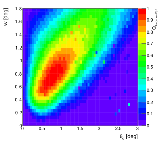
Figure 4: $\overline{\mathscr{Q}}$ as a function of $\theta_{\text{c}}$ and $w$, computed as an example from ${dN}/{d\Omega}$ from the Coma dSph defined in Bonnivard et al. (2015) and $\epsilon_{\text{MAGIC}}$.

In general, we want to compute the optimal pointing strategy taking all effects into account, the finite acceptance of the instrument, the leakage of signal between ON and OFF, and the finite angular resolution of the instrument. For that, we define $\overline{\mathscr{Q}}$

$$\overline{\mathscr{Q}}\left(w,\theta_{\text{c}}\right) = \mathscr{Q}_{Ac+Le+_{PSF}}\left(w,\theta_{\text{c}}\right)$$ (12)

$$= \frac{\int_{\Delta\Omega_{\text{ON}}}d\Omega_{\text{ON}}\;\mathcal{P}^{\prime}\left(\theta\right)\epsilon\left(d\right)-\int_{\Delta\Omega_{\text{OFF}}}d\Omega_{\text{OFF}}\;\mathcal{P}^{\prime}\left(\theta\right)\epsilon\left(d^{\prime}\right)}{\sqrt{\int_{\Delta\Omega_{\text{ON}}}d\Omega_{\text{ON}}\;\epsilon\left(d\right)}};$$

where $$d^{\prime}=\sqrt{\theta^{\prime 2}+w^{2}-2\cdot\theta^{\prime}\cdot w\cdot\cos(\varphi^{\prime})}\;\;\;\;(=d)$$

Figure 4 shows $\overline{\mathscr{Q}}$ as a function of the observational variables $w$ and $\theta_{\text{c}}$ for the Coma dSph (Bonnivard et al., 2015). $\overline{\mathscr{Q}}$ is a function of $\theta_{\text{c}}$ and $w$, and we define $w_{\text{opt}}$, $\theta_{\text{opt}}$ and their contour regions $\Delta w_{\text{opt}}$ and $\Delta\theta_{\text{opt}}$, as the values that maximize $\mathscr{Q}_{Ac}$ and that $\mathscr{Q}_{Ac}$ is within 30% of the maximum. The acceptance and the leakage effect have opposed tendencies w.r.t. $\theta_{\text{opt}}$ and $w_{\text{opt}}$, and the optimal region defined $\overline{\mathscr{Q}}$ defines a narrow region around them.

4 Optimized pointing strategy for indirect Dark Matter searches

IACTs core science is focused on the study of the cosmic ray origin in either Galactic or extragalactic targets, but it is well-known that cosmic gamma rays constitute also a probe for several fundamental physics investigations (including DM searches, see e.g. Doro et al., 2013). We can use Equation 12 to optimize the search of Weakly-Interacting Massive Particles  (WIMPs, generic massive particles postulated to solve the DM problem, see Boehm and Fayet, 2004; Griest and Kamionkowski, 1990) with Cherenkov telescopes.

The gamma-ray flux from annihilating (or decaying) WIMPs arriving at Earth from a given region of the sky ($\Delta\Omega$) can be factorized as

$$\frac{d\Phi(E,\Delta\Omega)}{dE}=\frac{d\overline{\Phi}^{\textrm{PP}}(E)}{dE}\cdot J(\Delta\Omega),$$ (13)

where $d\overline{\Phi}^{\textrm{PP}}/dE$ is called the particle-physics factor, and depends on the nature of DM, and $J(d\Omega)$ is called the astrophysics factor (or simply $J$-factor), and depends on the target distance and the DM distribution therein. These two factors read:

$$\frac{d\overline{\Phi}^{\textrm{PP}}(E)}{dE} = \frac{1}{4\pi}\frac{\alpha}{k\,m_{\mathrm{DM}}^{k}}\frac{dN}{dE}(E)$$

$$J(\Delta\Omega) = \int_{d\Omega}d\Omega\ \frac{dJ(l,\Omega)}{d\Omega}\;,$$ (14)

where $$\>\frac{dJ(l,\Omega)}{d\Omega}=\int_{\mathrm{l.o.s.}}dl\,\rho^{k}(l,\Omega)$$

respectively, with

$$\alpha=\langle\sigma\mathit{v}\rangle,k=2$$ , for annihilating DM,

$$\alpha=\tau^{-1},k=1$$ , for decaying DM;

$\langle\sigma\mathit{v}\rangle$, $\tau$ and $m_{\mathrm{DM}}$ are the DM particle velocity-averaged annihilation cross section, lifetime, and mass, respectively; $dN/dE$ is the average gamma-ray spectrum of a DM annihilation or decay event; and $\rho$ the DM density at a given sky direction $\Omega$ and distance from Earth $l$. The integrals in the astrophysical factor run over the region $\Delta\Omega$ and the line of sight, respectively; $\rho$ is typically assumed to be spherically symmetric, i.e. $\rho=\rho(r)$.

The DM signal profile $\mathcal{P}$ is determined by the $J$-factor:

$$\mathcal{P}\propto\frac{dJ}{d\Omega}.$$ (15)

The proportionality constant is absorbed in $\mathcal{A}$ (see Equation 6). Thus, using Equation 15 in Equation 12, we can optimize $w$ and $\theta_{\text{c}}$ for DM observations. Bonnivard et al. (2015) and Geringer-Sameth et al. (2015) provide the $J$-factor for two sets of DM halos hosting Milky Way dSphs, as a function of the signal integration angle ($\theta_{\text{c}}$). We apply the method to optimize the pointing strategy of annihilating and decaying DM for all available dSphs from both authors to be observed with MAGIC and CTA taking into account the three effects introduced in Equation 12 (acceptance, leakage and PSF).

	MAGIC				CTA
source	$\theta_{\text{opt}}$		$w_{\text{opt}}$		$\theta_{\text{opt}}$		$w_{\text{opt}}$
boo1	0.20	(0.10, 0.45)	0.30	(0.15, 0.60)	0.20	(0.10, 0.65)	0.55	(0.15, 1.16)
car	0.15	(0.10, 0.30)	0.25	(0.10, 0.55)	0.15	(0.10, 0.35)	0.40	(0.10, 1.16)
coma	0.25	(0.10, 0.60)	0.35	(0.20, 0.65)	0.35	(0.15, 0.95)	0.65	(0.30, 1.21)
cvn1	0.15	(0.10, 0.30)	0.25	(0.10, 0.55)	0.15	(0.10, 0.30)	0.40	(0.10, 1.16)
cvn2	0.15	(0.10, 0.35)	0.30	(0.10, 0.55)	0.15	(0.10, 0.35)	0.40	(0.10, 1.16)
dra	0.25	(0.10, 0.50)	0.35	(0.20, 0.65)	0.30	(0.10, 0.80)	0.60	(0.25, 1.16)
for	0.15	(0.10, 0.30)	0.25	(0.10, 0.55)	0.15	(0.10, 0.35)	0.45	(0.10, 1.16)
her	0.20	(0.10, 0.40)	0.30	(0.15, 0.55)	0.20	(0.10, 0.50)	0.50	(0.15, 1.16)
leo1	0.15	(0.10, 0.30)	0.25	(0.10, 0.55)	0.15	(0.10, 0.30)	0.35	(0.10, 1.16)
leo2	0.15	(0.10, 0.30)	0.25	(0.10, 0.55)	0.15	(0.10, 0.30)	0.35	(0.10, 1.16)
leo4	0.15	(0.10, 0.30)	0.25	(0.10, 0.55)	0.15	(0.10, 0.35)	0.45	(0.10, 1.16)
leo5	0.15	(0.10, 0.35)	0.30	(0.10, 0.55)	0.15	(0.10, 0.40)	0.45	(0.10, 1.16)
leot	0.15	(0.10, 0.30)	0.25	(0.10, 0.55)	0.15	(0.10, 0.30)	0.30	(0.10, 1.16)
scl	0.15	(0.10, 0.30)	0.25	(0.10, 0.55)	0.15	(0.10, 0.30)	0.35	(0.10, 1.16)
seg1	0.25	(0.10, 0.50)	0.35	(0.20, 0.60)	0.30	(0.10, 0.75)	0.55	(0.25, 1.16)
seg2	0.25	(0.10, 0.55)	0.35	(0.20, 0.65)	0.35	(0.15, 0.95)	0.65	(0.30, 1.21)
sex	0.25	(0.10, 0.55)	0.35	(0.20, 0.65)	0.35	(0.15, 0.85)	0.60	(0.25, 1.21)
uma1	0.15	(0.10, 0.30)	0.25	(0.10, 0.55)	0.15	(0.10, 0.35)	0.45	(0.10, 1.16)
uma2	0.35	(0.15, 0.75)	0.45	(0.25, 0.75)	0.50	(0.20, 1.10)	0.70	(0.35, 1.26)
umi	0.15	(0.10, 0.30)	0.25	(0.10, 0.55)	0.15	(0.10, 0.30)	0.40	(0.10, 1.16)
wil1	0.15	(0.10, 0.30)	0.25	(0.10, 0.55)	0.15	(0.10, 0.30)	0.40	(0.10, 1.16)

Table 1: List of optimal pointing wobble distance ($w_{\text{opt}}$) and signal region radius ($\theta_{\text{opt}}$), and their contour regions defined within 30% of the maximum of $\overline{\mathscr{Q}}$, for annihilating WIMP based on ${dJ}/{d\Omega}$ taken from Bonnivard et al. (2015). First column show the dSph name (taken from Bonnivard et al. (2015)). Second and third (fourth and fifth) show the optimal $\theta_{\text{c}}$ and $w$ for observations with MAGIC (CTA).

	MAGIC				CTA
source	$\theta_{\text{opt}}$		$w_{\text{opt}}$		$\theta_{\text{opt}}$		$w_{\text{opt}}$
boo	0.20	(0.10, 0.40)	0.30	(0.15, 0.55)	0.25	(0.10, 0.45)	0.35	(0.20, 1.16)
car	0.15	(0.10, 0.35)	0.30	(0.10, 0.55)	0.15	(0.10, 0.45)	0.45	(0.15, 1.16)
coma	0.15	(0.10, 0.30)	0.25	(0.10, 0.55)	0.15	(0.10, 0.30)	0.30	(0.10, 1.16)
cvn1	0.15	(0.10, 0.40)	0.30	(0.15, 0.55)	0.20	(0.10, 0.45)	0.35	(0.15, 1.16)
cvn2	0.15	(0.05, 0.25)	0.20	(0.10, 0.55)	0.15	(0.05, 0.20)	0.30	(0.10, 1.16)
dra	0.25	(0.10, 0.55)	0.35	(0.20, 0.65)	0.35	(0.15, 0.85)	0.60	(0.25, 1.16)
for	0.15	(0.10, 0.35)	0.25	(0.10, 0.55)	0.15	(0.10, 0.35)	0.35	(0.10, 1.16)
her	0.15	(0.05, 0.25)	0.25	(0.10, 0.55)	0.15	(0.05, 0.25)	0.30	(0.10, 1.16)
leo1	0.15	(0.10, 0.35)	0.25	(0.10, 0.55)	0.15	(0.10, 0.40)	0.35	(0.15, 1.16)
leo2	0.15	(0.05, 0.25)	0.25	(0.10, 0.55)	0.15	(0.05, 0.25)	0.30	(0.10, 1.16)
leo4	0.15	(0.05, 0.25)	0.20	(0.10, 0.55)	0.15	(0.05, 0.20)	0.30	(0.10, 1.16)
leo5	0.15	(0.05, 0.20)	0.20	(0.10, 0.55)	0.10	(0.05, 0.20)	0.35	(0.10, 1.16)
leot	0.15	(0.05, 0.20)	0.20	(0.10, 0.55)	0.10	(0.05, 0.20)	0.35	(0.10, 1.16)
scl	0.15	(0.10, 0.35)	0.30	(0.15, 0.55)	0.15	(0.10, 0.45)	0.40	(0.15, 1.16)
seg1	0.15	(0.10, 0.30)	0.25	(0.10, 0.55)	0.15	(0.10, 0.35)	0.30	(0.10, 1.16)
seg2	0.15	(0.05, 0.25)	0.25	(0.10, 0.55)	0.15	(0.05, 0.25)	0.30	(0.10, 1.16)
sex	0.30	(0.10, 0.65)	0.40	(0.20, 0.70)	0.50	(0.15, 1.10)	0.75	(0.35, 1.21)
uma1	0.15	(0.10, 0.35)	0.25	(0.15, 0.55)	0.20	(0.10, 0.40)	0.35	(0.15, 1.16)
uma2	0.25	(0.10, 0.45)	0.30	(0.20, 0.55)	0.30	(0.10, 0.50)	0.40	(0.20, 1.16)
umi	0.15	(0.05, 0.25)	0.25	(0.10, 0.55)	0.15	(0.05, 0.25)	0.35	(0.10, 1.16)

Table 2: List of optimal pointing wobble distance ($w_{\text{opt}}$) and signal region radius ($\theta_{\text{opt}}$) for annihilating WIMP based on ${dJ}/{d\Omega}$ Geringer-Sameth et al. (2015). Column description can be found in Table 1.

We focus first on the annihilation case, and provide the optimal values $w_{\text{opt}}$, $\theta_{\text{opt}}$, and their 30% variation ranges in Table 1 and 2.

For the case of MAGIC, we note how $w_{\text{opt}}$ is systematically lower than $w_{\text{MAGIC}}=0.4^{\circ}$. This is the case for most point-like sources, for which, in the case of the standard analysis of MAGIC, 3 different off regions are considered, and therefore, for the same $w$, the distance between these OFF regions and the ON is smaller. There are a few cases in which the source appears to be moderately extended for MAGIC, i.e. uma2 (in Bonnivard et al., 2015) or sex (in Geringer-Sameth et al., 2015). The discrepancies between the optimal values obtained (for the same source) from the two authors show the large uncertainties affecting the DM profiles. Finally, it should also be said that, for the sake of simplicity, the method does not take into account systematic effects that may affect the real analysis. For instance, the systematic error on the background estimation, is proportional to the number of OFF events. This means that for two different configurations (two different $w$ and $\theta_{\text{c}}$ pairs) with similar $\mathscr{Q}$, we should give priority to the one with lower $\theta_{\text{c}}$ (lower statistics).

For the case of CTA, our results can be taken as reference to schedule future observations. However two caveats should be considered: 1) CTA will be composed of two sites, one operating in the North (CTAN) hemisphere and one in the south (CTAS) however, we treated all dSphs with the same instrument acceptance regardless of their position in the sky; 2) Each CTA site (CTAN and CTAS) will be integrated by, up to, three different types of telescope and hence, once CTA analysis scheme is defined, a proper optimization could be performed for the pointing of each telescope using our code.

	MAGIC				CTA
source	$\theta_{\text{opt}}$		$w_{\text{opt}}$		$\theta_{\text{opt}}$		$w_{\text{opt}}$
boo1	0.50	(0.20, 0.85)	0.50	(0.30, 0.90)	0.65	(0.25, 1.30)	0.85	(0.45, 1.30)
car	0.30	(0.10, 0.65)	0.40	(0.20, 0.70)	0.50	(0.15, 1.10)	0.75	(0.35, 1.30)
coma	0.50	(0.25, 0.85)	0.50	(0.35, 0.90)	0.70	(0.30, 1.70)	0.91	(0.50, 1.40)
cvn1	0.25	(0.10, 0.65)	0.40	(0.20, 0.70)	0.45	(0.15, 1.10)	0.70	(0.35, 1.20)
cvn2	0.30	(0.15, 0.65)	0.40	(0.20, 0.70)	0.45	(0.15, 1.00)	0.70	(0.30, 1.20)
dra	0.50	(0.20, 0.95)	0.55	(0.35, 0.90)	0.75	(0.25, 1.20)	0.75	(0.50, 1.30)
for	0.35	(0.15, 0.70)	0.45	(0.25, 0.75)	0.50	(0.20, 1.10)	0.70	(0.35, 1.30)
her	0.50	(0.20, 0.95)	0.55	(0.30, 0.90)	0.65	(0.25, 1.20)	0.80	(0.45, 1.30)
leo1	0.25	(0.10, 0.55)	0.35	(0.20, 0.65)	0.35	(0.15, 1.00)	0.70	(0.30, 1.20)
leo2	0.20	(0.10, 0.50)	0.30	(0.15, 0.60)	0.25	(0.10, 0.75)	0.60	(0.20, 1.20)
leo4	0.30	(0.10, 0.65)	0.40	(0.20, 0.65)	0.50	(0.15, 1.00)	0.70	(0.35, 1.20)
leo5	0.30	(0.10, 0.65)	0.40	(0.20, 0.70)	0.50	(0.15, 1.10)	0.70	(0.35, 1.20)
leot	0.20	(0.10, 0.40)	0.30	(0.15, 0.60)	0.20	(0.10, 0.50)	0.50	(0.15, 1.20)
scl	0.25	(0.10, 0.50)	0.35	(0.20, 0.65)	0.30	(0.10, 0.90)	0.65	(0.25, 1.20)
seg1	0.50	(0.15, 0.95)	0.55	(0.30, 0.90)	0.65	(0.25, 1.30)	0.85	(0.45, 1.30)
seg2	0.70	(0.30, 1.10)	0.65	(0.40, 1.10)	0.70	(0.30, 1.30)	0.85	(0.45, 1.40)
sex	0.65	(0.30, 1.20)	0.70	(0.40, 1.00)	0.70	(0.30, 5.50)	0.85	(0.50, 1.40)
uma1	0.30	(0.15, 0.65)	0.40	(0.20, 0.70)	0.50	(0.20, 1.10)	0.70	(0.35, 1.30)
uma2	5.60	(1.10, 5.60)	1.20	(1.20, 1.20)	6.50	(0.60, 6.50)	1.40	(1.40, 1.40)
umi	0.30	(0.10, 0.65)	0.40	(0.20, 0.70)	0.50	(0.15, 1.10)	0.70	(0.35, 1.30)
wil1	0.30	(0.10, 0.70)	0.45	(0.20, 0.70)	0.50	(0.15, 1.10)	0.70	(0.35, 1.20)

Table 3: List of optimal pointing wobble distance ($w_{\text{opt}}$) and signal region radius ($\theta_{\text{opt}}$) for decaying WIMP based on ${dJ}/{d\Omega}$ based on Bonnivard et al. (2015). Column description can be found in Table 1.

	MAGIC				CTA
source	$\theta_{\text{opt}}$		$w_{\text{opt}}$		$\theta_{\text{opt}}$		$w_{\text{opt}}$
boo	0.25	(0.15, 0.45)	0.30	(0.20, 0.55)	0.30	(0.15, 0.50)	0.40	(0.20, 1.16)
car	0.30	(0.15, 0.65)	0.40	(0.25, 0.70)	0.45	(0.15, 0.95)	0.65	(0.35, 1.16)
coma	0.20	(0.10, 0.35)	0.25	(0.15, 0.55)	0.15	(0.10, 0.35)	0.30	(0.10, 1.16)
cvn1	0.25	(0.10, 0.45)	0.30	(0.20, 0.60)	0.30	(0.15, 0.50)	0.40	(0.20, 1.16)
cvn2	0.15	(0.05, 0.25)	0.25	(0.10, 0.55)	0.15	(0.05, 0.20)	0.30	(0.10, 1.16)
dra	0.80	(0.35, 1.15)	0.75	(0.45, 1.00)	0.65	(0.30, 1.15)	0.75	(0.45, 1.21)
for	0.25	(0.10, 0.50)	0.35	(0.20, 0.60)	0.30	(0.15, 0.65)	0.50	(0.20, 1.16)
her	0.15	(0.10, 0.30)	0.25	(0.10, 0.55)	0.15	(0.10, 0.30)	0.30	(0.10, 1.16)
leo1	0.25	(0.10, 0.45)	0.30	(0.20, 0.55)	0.25	(0.10, 0.45)	0.35	(0.20, 1.16)
leo2	0.15	(0.05, 0.25)	0.25	(0.10, 0.55)	0.15	(0.05, 0.25)	0.30	(0.10, 1.16)
leo4	0.15	(0.05, 0.25)	0.25	(0.10, 0.55)	0.15	(0.05, 0.25)	0.30	(0.10, 1.16)
leo5	0.15	(0.05, 0.25)	0.20	(0.10, 0.55)	0.10	(0.05, 0.20)	0.35	(0.10, 1.16)
leot	0.15	(0.05, 0.25)	0.20	(0.10, 0.55)	0.15	(0.05, 0.20)	0.30	(0.10, 1.16)
scl	0.30	(0.15, 0.65)	0.40	(0.20, 0.65)	0.40	(0.15, 0.90)	0.65	(0.30, 1.21)
seg1	0.20	(0.10, 0.35)	0.25	(0.15, 0.55)	0.20	(0.10, 0.35)	0.30	(0.15, 1.16)
seg2	0.15	(0.05, 0.25)	0.25	(0.10, 0.55)	0.15	(0.05, 0.25)	0.30	(0.10, 1.16)
sex	0.90	(0.45, 1.35)	0.85	(0.55, 1.20)	0.80	(0.35, 1.45)	0.91	(0.55, 1.31)
uma1	0.25	(0.10, 0.45)	0.30	(0.20, 0.55)	0.25	(0.10, 0.45)	0.35	(0.20, 1.16)
uma2	0.30	(0.15, 0.50)	0.35	(0.20, 0.60)	0.35	(0.15, 0.55)	0.40	(0.25, 1.16)
umi	0.20	(0.10, 0.45)	0.30	(0.15, 0.60)	0.25	(0.10, 0.60)	0.50	(0.20, 1.16)

Table 4: List of optimal pointing wobble distance ($w_{\text{opt}}$) and signal region radius ($\theta_{\text{opt}}$) for decaying WIMP based on ${dJ}/{d\Omega}$ based on Geringer-Sameth et al. (2015). Column description can be found in Table 1.

Tables 3 and 4 show the optimal values ($w_{\text{opt}}$, $\theta_{\text{opt}}$) for the decay case.

Most of these sources are considered to be rather extended (this is expected given the dependence on $\rho$ in section 4).

5 Summary and Discussion

In this work, we have proposed a method to optimize the pointing strategy and analysis for extended sources observed by IACTs. The method provides the optimal offset and signal integration distances ($w_{\text{opt}},\theta_{\text{opt}}$) taking into account: the off-axis performance and the angular resolution of the instrument, and the profile of the source under observation. The method has a potential use in scheduling new observations, but can also be used to optimize the analysis cut $\theta_{\text{c}}$ (typically used by the community as a cut on $\theta^{2}$) for data already taken. We focus on the case of indirect DM searches, and provide optimal pointing strategies for indirect DM searches on a set of dSph to be observed with MAGIC and CTA.

We have implemented the method in a tool that is freely distributed, open source software, accessible from:

• https://github.com/IndirectDarkMatterSearchesIFAE/

A released version (V1.0), with which the results shown in this paper were computed, can be accessed by:

• $ git clone https://github.com/IndirectDarkMatterSearchesIFAE/ObservationOptimization.git

• $ git checkout V1.0

The package is provided with tutorials in order to acquire the basic skills required to reproduce the results shown here. The software is flexible enough so that new sources (not necessary related to DM) or telescopes can be defined easily. This provides an easy, fast, and powerful tool for planning new observations with IACTs.

References

- Acharya et al. (2017) B. S. Acharya et al. Science with the Cherenkov Telescope Array. arXiv:1709.07997, 2017.
- Aleksić et al. (2012) J. Aleksić et al. Performance of the MAGIC stereo system obtained with Crab Nebula data. Astropart. Phys., 35:435–448, 2012. doi: 10.1016/j.astropartphys.2011.11.007.
- Aleksić et al. (2016) J. Aleksić et al. The major upgrade of the MAGIC telescopes, Part II: A performance study using observations of the Crab Nebula. Astropart. Phys., 72:76–94, 2016. doi: 10.1016/j.astropartphys.2015.02.005.
- Boehm and Fayet (2004) C. Boehm and P. Fayet. Scalar dark matter candidates. Nucl. Phys., B683:219–263, 2004. doi: 10.1016/j.nuclphysb.2004.01.015.
- Bonnivard et al. (2015) V. Bonnivard et al. Dark matter annihilation and decay in dwarf spheroidal galaxies: The classical and ultrafaint dSphs. Mon. Not. Roy. Astron. Soc., 453(1):849–867, 2015. doi: 10.1093/mnras/stv1601.
- Doro et al. (2013) M. Doro et al. Dark Matter and Fundamental Physics with the Cherenkov Telescope Array. Astropart. Phys., 43:189–214, 2013. doi: 10.1016/j.astropartphys.2012.08.002.
- Fomin et al. (1994) V. P. Fomin, A. A. Stepanian, R. C. Lamb, D. A. Lewis, M. Punch, and T. C. Weekes. New methods of atmospheric Cherenkov imaging for gamma-ray astronomy. I. The false source method. Astroparticle Physics, 2:137–150, May 1994. doi: 10.1016/0927-6505(94)90036-1.
- Geringer-Sameth et al. (2015) A. Geringer-Sameth, S. M. Koushiappas, and M. Walker. Dwarf galaxy annihilation and decay emission profiles for dark matter experiments. Astrophys. J., 801(2):74, 2015. doi: 10.1088/0004-637X/801/2/74.
- Griest and Kamionkowski (1990) K. Griest and M. Kamionkowski. Unitarity Limits on the Mass and Radius of Dark Matter Particles. Phys. Rev. Lett., 64:615, 1990. doi: 10.1103/PhysRevLett.64.615.
- Hassan et al. (2017) T. Hassan et al. Monte Carlo Performance Studies for the Site Selection of the Cherenkov Telescope Array. Astropart. Phys., 93:76–85, 2017. doi: 10.1016/j.astropartphys.2017.05.001.