Analyzing Diffusion and Flow-driven Instability
using Semidefinite Programming

Abstract

Diffusion and flow-driven instability, or transport-driven instability, is one of the central mechanisms to generate inhomogeneous gradient of concentrations in spatially distributed chemical systems. However, verifying the transport-driven instability of reaction-diffusion-advection systems requires checking the Jacobian eigenvalues of infinitely many Fourier modes, which is computationally intractable. To overcome this limitation, this paper proposes mathematical optimization algorithms that determine the stability/instability of reaction-diffusion-advection systems by finite steps of algebraic calculations. Specifically, the stability/instability analysis of Fourier modes is formulated as a sum-of-squares (SOS) optimization program, which is a class of convex optimization whose solvers are widely available as software packages. The optimization program is further extended for facile computation of the destabilizing spatial modes. This extension allows for predicting and designing the shape of concentration gradient without simulating the governing equations. The streamlined analysis process of self-organized pattern formation is demonstrated with a simple illustrative reaction model with diffusion and advection.

Keywords: reaction-diffusion-advection model, transport-driven instability, convex optimization, semidefinite programming, self-organized pattern formation

1 Introduction

Molecular transportation is a fundamental mechanism that couples spatially distributed chemical reaction networks and enables self-organized pattern formation in biology and chemistry. For example, in developmental biology, passive diffusion and advective flow of signaling molecules within and between cells are known to play a central role in identifying and regulating positions and shapes during embryo-genesis [1, 2, 3] and cell division [4, 5, 6, 7, 8]. In chemistry, diffusion-driven self-organized patterns were reconstituted in crafted reactors with commodity chemicals [9, 10]. More recently, synthetic biologists have been attempting to utilize quorum sensing, a mechanism of diffusion-based cell-to-cell signaling of E. coli, to regulate a population of synthetic biomolecular reaction systems that communicate [11, 12, 13, 14, 15] and synchronize with each other [16, 17, 18, 19].

The theoretical foundation of transport-driven self-organization was established by Turing [20], where he showed using a reaction-diffusion equation that molecular concentrations can form a spatially periodic gradient due to the interaction of reaction and diffusion despite the averaging nature of diffusion. Later, Rovinsky and Menzinger [21, 22] verified both mathematically and experimentally that differential flow, or advection, of molecules can also induce an oscillatory spatio-temporal concentration gradient. In these works, mathematical analyses revealed that the pattern formation was due to the destabilization of spatial oscillation modes, and the destabilization was induced by the difference of diffusion and flow rates between reactive molecules. Mathematically, this can be interpreted that molecular transportation caused spontaneous growth of some spatial Fourier modes and led to spatially periodic pattern formation at steady state.

Currently, a widely used approach to analyzing the transport-driven pattern formation is the linear stability/instability analysis of spatial Fourier components. Specifically, the Jacobian eigenvalues of the governing reaction-diffusion-advection equations are computed for different spatial Fourier modes to explore the existence of unstable harmonic components. Then, spatially periodic pattern formation is expected if an eigenvalue of the Jacobian resides in the right-half complex plane for some non-zero frequency components. For relatively simple reaction systems, analytic instability conditions were obtained using this approach, and the parameter space for pattern formation was thoroughly characterized [23, 1, 24]. For large-scale and complex reaction systems, on the other hand, instability analysis requires substantial computational efforts to iteratively compute Jacobian eigenvalues for each Fourier component. However, this approach is essentially incapable of drawing mathematically rigorous conclusion on the stability of reaction-diffusion-advection systems since the spatial gradient of chemical concentrations is represented with infinitely many Fourier modes.

Another approach to analyzing the stability/instability of reaction-diffusion equations is to use Lyapunov’s method, where the core idea is to guarantee the energy dissipation of certain Fourier components by constructing a Lyapunov function. The exploration of a Lyapunov function typically reduces to an algebraic optimization problem called semidefinite programming (SDP), which is an efficiently solvable class of convex optimization [25, 26]. Existing works presented sufficient conditions for the stability of reaction-diffusion equations, certifying non-existence of spatially inhomogeneous solutions [27, 28, 29]. A more general SDP based framework was also developed for the stability analysis of univariate nonlinear partial differential equations by exploring polynomial integral Lyapunov functions [30]. However, the focus of these works is spatially homogeneous behavior, and the conditions are not necessarily suitable for studying diffusion-driven instability that leads to spatially periodic pattern formation.

This paper presents computationally tractable necessary and sufficient conditions for the local stability/instability of reaction-diffusion-advection systems. The proposed approach is amenable to computational implementation and is particularly convenient for analyzing transport-driven instability. Specifically, we derive linear matrix inequality (LMI) conditions that certify the stability/instability of infinitely many Fourier components. This algebraic condition can be efficiently verified with semidefinite programming (SDP) [25, 26]. The derivation of these conditions is based on the linear stability analysis of Fourier components. Although the analysis essentially requires checking the roots of infinitely many characteristic polynomials with complex coefficients, we show that the local stability is equivalent to an existence of sum-of-squares (SOS) decomposition of certain Hurwitz polynomials, which can be formulated as a semidefinite optimization problem [31]. Based on this result, we further derive conditions for certifying the stability/instability of reaction-diffusion-advection systems for a prespecified set of spatial frequency. This extension allows for facile computation of the destabilizing spatial modes, enabling the prediction of spatial oscillations without simulating the governing equation. The proposed instability analysis helps not only better understanding of reaction-diffusion-advection kinetics but also engineering of chemical reactions in synthetic biology and chemistry.

The following notations are used in this paper. $\mathbb{N}$ is a set of positive integers. $\mathbb{Z}$ is a set of all integers. $\mathbb{R}$ is a set of real numbers. $\mathbb{R}^{{n}\times{n}}$ is a set of $n$ by $n$ matrices with real entries. $|A|$ is a determinant of the matrix $A$. $A\succeq O$ means that $A$ is positive semidefinite. $\mathrm{deg}(p(x))$ is the degree of a polynomial $p(x)$. $\lceil x\rceil$ is the ceiling function, that is, the smallest integer that is greater than or equal to $x$.

2 Model of reaction-diffusion-advection system

We consider a reaction-diffusion-advection process of $n$ molecular species defined in a finite spatial domain $\Omega$. For notational simplicity, we consider only one dimensional space $\Omega:=[0,L]$, whose coordinate is specified by the symbol $x$, but all theoretical results shown in this paper can be generalized to higher dimensions. Let $C_{i}(x,t)$ denote the concentration of the $i$-th molecule at position $x\in\Omega$ and time $t$ and ${\bm{C}}(x,t)$ be the vector of the molecular concentrations ${\bm{C}}(x,t):=[C_{1}(x,t),C_{2}(x,t),\cdots,C_{n}(x,t)]^{T}$. The spatio-temporal dynamics of the molecular concentrations are then described by the reaction-diffusion-advection equation

$$\frac{\partial{\bm{C}}(x,t)}{\partial t}={\bm{f}}({\bm{C}}(x,t))+D\frac{\partial^{2}{\bm{C}}(x,t)}{\partial x^{2}}+V\frac{\partial{\bm{C}}(x,t)}{\partial x},$$ (1)

where the function ${\bm{f}}(\cdot)$ is a $C^{1}$ vector-valued function governing local reactions, and $D:=\mathrm{diag}(d_{1},d_{2},\cdots,d_{n})$ and $V:=\mathrm{diag}(v_{1},v_{2},\cdots,v_{n})$ are the coefficients of diffusion and flow velocity, respectively. We assume $d_{i}>0$ and $v_{i}\geq 0$ in the following theoretical development $(i=1,2,\cdots,n)$.

The reaction-diffusion-advection system shows a variety of spatio-temporal dynamics ranging from spatially uniform steady state to spatio-temporal oscillations depending on the parameters and the stoichiometry of the reactions. As a motivating example, we consider the following set of reactions that consists of molecules $P$, $Q$, and a product $R$:

$$\ce{P+2Q->3Q},~{}~{}~{}~{}\ce{Q->R},$$ (2)

where the molecule $Q$ catalyzes its own production using the substrate $P$, and the product $R$ is inert to the reactions [32, 33]. The substrate $P$ is constantly supplied at a constant rate and all molecules are drained at the same rate as illustrated in Fig. 1(A). We assume that all molecules are spatially distributed in one dimensional space $\Omega:=[0,30\pi]$ with periodic boundary conditions, and they are transported by constant flow and passive diffusion. The spatio-temporal dynamics of the molecular concentrations are then modeled by

$$\begin{array}[]{l}\displaystyle\frac{\partial C_{1}}{\partial t}=-C_{1}C_{2}^{2}+a(1-C_{1})+d\frac{\partial^{2}C_{1}}{\partial x^{2}}+v_{1}\frac{\partial C_{1}}{\partial x},\\ \displaystyle\frac{\partial C_{2}}{\partial t}=C_{1}C_{2}^{2}-(a+b)C_{2}+\frac{\partial^{2}C_{2}}{\partial x^{2}}+v_{2}\frac{\partial C_{2}}{\partial x},\end{array}$$ (3)

where $C_{1}(x,t)$ and $C_{2}(x,t)$ denote the concentrations of $P$ and $Q$, respectively. In the model (3), the reaction rates are normalized by that of the autocatalytic reaction in (2). The constant $a$ and $b$ represent the normalized supply rate of the substrate $P$ and the production rate of $R$ (see Fig. 1(A)). The spatial coordinate $x$ is defined so that the diffusion coefficient of the molecule $Q$ becomes one.

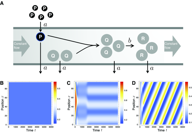
Figure 1: A reaction-diffusion-advection system inducing flow-driven instability (A) Schematics of the reaction model with diffusion and advection. (B-D) Spatio-temporal dynamics of concentration gradient for different values of parameters.

Fig. 1(B)-(D) illustrate qualitatively different spatio-temporal dynamics for the reaction-diffusion-advection system (3) for different choices of $b$, $v_{1}$ and $v_{2}$. Specifically, $(b,v_{1},v_{2})=(0.040,0,0)$ for Fig. 1(B), $(b,v_{1},v_{2})=(0.055,0,0)$ for Fig. 1(C), and $(b,v_{1},v_{2})=(0.040,1.897,0.3162)$ for Fig. 1(D) were used (see Method section for the other parameters and initial values). The concentration of $P$ forms spatially periodic oscillations as $b$ increases from $0.040$ to $0.055$ despite the averaging effect of the passive diffusion (Fig. 1(B), (C)). This pattern formation, which is widely known as Turing pattern formation, is caused by the destabilization of certain spatial oscillation modes due to the difference of the diffusion rates (diffusion instability) [2]. On the other hand, the spatio-temporal oscillations in Fig. 1(D) is induced by a different destabilization mechanism based on the advective transportation of the molecules.

In the following sections, we first review that these destabilizing effects can be explained by probing the local instability of Fourier modes of the reaction-diffusion-advection system. We then present novel algebraic stability conditions for the stability/instability analysis of infinitely many Fourier modes with semidefinite programming.

3 Stability analysis of spatial Fourier components

To analyze instability of spatial modes associated with spatial pattern formation, we linearize the equation (1) around a spatially homogeneous equilibrium point ${\bm{C}}(x,t)=\bar{{\bm{C}}}$. In other words, $\bar{{\bm{C}}}$ is an equilibrium of local reactions satisfying ${\bm{f}}(\bar{{\bm{C}}})=0$. Assuming the existence of such equilibrium point, we can write the evolution of the molecular concentrations around $\bar{{\bm{C}}}$ by

$$\frac{\partial{\bm{c}}(x,t)}{\partial t}=A{\bm{c}}(x,t)+D\frac{\partial^{2}{\bm{c}}(x,t)}{\partial x^{2}}+V\frac{\partial{\bm{c}}(x,t)}{\partial x},$$ (4)

where ${\bm{c}}(x,t):={\bm{C}}(x,t)-\bar{\bm{C}}$ is the vector of relative concentrations, and $A$ is the Jacobian of ${\bm{f}}(\cdot)$ evaluated at $\bar{{\bm{C}}}$.

The local behavior of ${\bm{c}}(x,t)$ can be characterized by its spatial Fourier components $\tilde{\bm{c}}(\zeta,t)$ when the boundaries of the spatial domain $\partial\Omega$ satisfy certain conditions. Specifically, let $\tilde{\bm{c}}(\zeta,t)$ be the Fourier coefficients of ${\bm{c}}(x,t)$ satisfying

$${\bm{c}}(x,t)=\sum_{\zeta\in\mathcal{Z}}\tilde{\bm{c}}(\zeta,t)e^{j\zeta x},$$ (5)

where $\mathcal{Z}$ is a set of discrete frequency variables that depends on the boundary conditions (see Remark 1). Multiplying by $e^{-j\zeta x}$ and taking the integral of both sides of (4), we have

$$\frac{d\tilde{{\bm{c}}}(\zeta,t)}{dt}=(A-\zeta^{2}D+j\zeta{V})\tilde{{\bm{c}}}(\zeta,t).$$ (6)

This equation represents the dynamics of frequency component $\tilde{{\bm{c}}}(\zeta,t)$. It should be noticed that, for each fixed $\zeta$, (6) is an $n$-th order linear time-invariant ordinary differential equation (ODE) with complex coefficients. Thus, the reaction-diffusion-advection equation is decomposed into a set of infinitely many ODEs.

Remark 1. The frequency variable $\zeta$ in (5) takes discrete values that depend on the boundary conditions. Specifically, let the set of all frequency variables for a given boundary condition be denoted by $\mathcal{Z}$. Then, $\mathcal{Z}=\{2k\pi/L\}_{k\in\mathbb{Z}}$ for periodic boundary conditions. When $V=O$, $\mathcal{Z}$ is defined by $\mathcal{Z}=\{k\pi/L\}_{k\in\mathbb{Z}}$ for the Neumann boundary condition and $\mathcal{Z}=\{k\pi/L\}_{k\in\mathbb{Z}\backslash\{0\}}$ for the Dirichlet boundary condition, respectively [34]. The reader is referred to [34] for other boundary conditions. It should also be noted that $\mathrm{Im}[\tilde{\bm{c}}(\zeta,t)]=0$ for the Neumann boundary with $V=0$ and $\mathrm{Re}[\tilde{\bm{c}}(\zeta,t)]=0$ for the Dirichlet boundary with $V=0$, implying that the Fourier cosine and sine transforms are used to obtain $\tilde{\bm{c}}(\zeta,t)$, respectively.

Since the equation (6) represents the dynamics of Fourier components, ${\bm{c}}(x,t)$ asymptotically converges to zero if the growth rate of $\tilde{{\bm{c}}}(\zeta,t)$ is negative for all frequency components $\zeta$. On the other hand, if there exists a frequency component $\tilde{{\bm{c}}}(\zeta,t)$ with non-zero frequency $\zeta$ whose growth rate is positive, the corresponding non-zero spatial mode is amplified around the spatially homogeneous equilibrium $\bar{{\bm{C}}}$. In the nonlinear reaction-diffusion-advection system (1), the unstable frequency component potentially induces periodic pattern formation in space. In other words, the existence of a growing frequency component with non-zero frequency is a necessary condition for the generation of spatially periodic pattern in the system (1).

More formally, this can be stated as local stability/instability of the nonlinear reaction-diffusion-advection system (1). The nonlinear system (1) is said to be locally stable around $\bar{{\bm{C}}}$ if the linear system (6) is asymptotically stable. For linear systems, asymptotic stability is determined from the eigenvalues of the matrix $A-\zeta^{2}D+j\zeta V$. More specifically, the following lemma holds (see Supplementary Information for the proof).

Lemma 1. Consider the linear reaction-diffusion-advection system (4). The system (4) is asymptotically stable if and only if all roots of the characteristic polynomial

$$\varphi(\zeta,s):=|sI-A+D\zeta^{2}-j\zeta V|=0$$ (7)

are in the open left-half complex plane $\{s\in\mathbb{C}~{}|~{}\mathrm{Re}[s]<0\}$ for all $\zeta\in\mathcal{Z}$, where $\mathcal{Z}$ is defined in Remark 1.

Thus, the stability analysis of the reaction-diffusion-advection system (4) reduces to finding the roots of the polynomial $\varphi(\zeta,s)=0$ for $\zeta\in\mathcal{Z}$. It should, however, be noted that verifying the stability condition requires solving infinitely many polynomial equations with complex coefficients (7), and analytic conditions are hardly obtained except for some special cases [21, 35]. Consequently, most of the existing works resort to approximate stability analysis by solving (7) for a finite range of quantized $\zeta$. In the next section, we propose a novel computational approach that overcomes this limitation. Specifically, we introduce a computationally tractable optimization problem that certifies the stability of the reaction-diffusion-advection system.

4 Linear matrix inequality condition for stability/instability analysis

In this section, we show matrix inequality conditions for computational verification of the stability/instability of the system (4). For theoretical development, we here consider a slightly modified condition of Lemma 1 that all roots of the polynomial (7) lie in the open left-half complex plane for $\zeta\in\mathbb{R}$ instead of $\zeta\in\mathcal{Z}$. Mathematically, this becomes only a sufficient condition for the asymptotic stability of the system (4). However, conventionally, this condition has been used for the stability/instability analysis of reaction-diffusion-advection systems [20, 21, 22] since the elements of $\mathcal{Z}$, which lie on the real axis $(-\infty,\infty)$ tend to be close to each other as the length of the domain $L$ becomes large, and the gap from the necessary condition becomes small enough in practical applications.

To this end, we first review an algebraic stability condition due to Hurwitz (Theorem 3.4.68 of [36]). Let $\varphi_{\rm Re}(\zeta,s)$ and $\varphi_{\rm Im}(\zeta,s)$ be real and imaginary parts of the complex polynomial $\varphi(\zeta,js)$, respectively. Specifically, we denote by

$$\varphi(\zeta,js)=\varphi_{\rm Re}(\zeta,s)+j\varphi_{\rm Im}(\zeta,s)$$ (8)

with

$$\varphi_{\rm Re}(\zeta,s)=p_{n}(\zeta)s^{n}+p_{n-1}(\zeta)s^{n-1}+p_{n-2}(\zeta)s^{n-2}+\cdots+p_{0}(\zeta),$$

$$\varphi_{\rm Im}(\zeta,s)=q_{n}(\zeta)s^{n}+q_{n-1}(\zeta)s^{n-1}+q_{n-2}(\zeta)s^{n-2}+\cdots+q_{0}(\zeta),$$

where $p_{i}(\zeta)$ and $q_{i}(\zeta)$ are polynomials of $\zeta$ with real coefficients. Note that $\varphi_{{\rm Re}}(\zeta,s)$ and $\varphi_{{\rm Im}}(\zeta,s)$ are not defined for $\varphi(\zeta,s)$ but for $\varphi(\zeta,js)$ in (8). Using these polynomials, we define the following $2n\times 2n$ Sylvester matrix

$$S:=\begin{bmatrix}q_{n}&q_{n-1}&q_{n-2}&\cdots&\cdots&q_{0}&0&\cdots&0\\ p_{n}&p_{n-1}&p_{n-2}&\cdots&\cdots&p_{0}&0&\cdots&0\\ 0&q_{n}&q_{n-1}&q_{n-2}&\cdots&\cdots&q_{0}&\cdots&0\\ 0&p_{n}&p_{n-1}&p_{n-2}&\cdots&\cdots&p_{0}&\cdots&0\\ \vdots&\ddots&\ddots&\ddots&\ddots&\ddots&\ddots&\ddots&\vdots\\ 0&\cdots&\cdots&\cdots&q_{n}&q_{n-1}&q_{n-2}&\cdots&q_{0}\\ 0&\cdots&\cdots&\cdots&p_{n}&p_{n-1}&p_{n-2}&\cdots&p_{0}\end{bmatrix}$$ (9)

and define $2i$-th order principal minors of the matrix by $\Delta_{i}(\zeta)~{}(i=1,2,\cdots,n)$. For example,

$$\Delta_{1}(\zeta)=\left|\begin{array}[]{cccc}q_{n}&q_{n-1}\\ p_{n}&p_{n-1}\end{array}\right|,~{}\Delta_{2}(\zeta)=\left|\begin{array}[]{cccc}q_{n}&q_{n-1}&q_{n-2}&q_{n-3}\\ p_{n}&p_{n-1}&p_{n-2}&p_{n-3}\\ 0&q_{n}&q_{n-1}&q_{n-2}\\ 0&p_{n}&p_{n-1}&p_{n-2}\end{array}\right|$$ (16)

and $\Delta_{n}=|S|$.

According to the Hurwitz criterion for complex polynomials (Theorem 3.4.68 of [36]), all roots of $\varphi(\zeta,s)=0$ lie in the open left-half complex plane for a given $\zeta$ if and only if the coefficients satisfy the polynomial inequalities $\Delta_{i}(\zeta)>0~{}(i=1,2,\cdots,n)$. Thus, for each fixed value of $\zeta$, we can check the stability of the corresponding Fourier mode using computationally tractable algebraic conditions. To analyze the stability of the reaction-diffusion-advection system (4), however, we need to guarantee the stability for all frequency $\zeta$, which is computationally intractable. As a result, the stability analysis of the reaction-diffusion-advection system often resorts to approximation by iteratively checking the sign of $\Delta_{i}(\zeta)$ for a finite range of discretized values of $\zeta$. To overcome this issue, we introduce a computationally tractable condition for certifying non-negativity of $\Delta_{i}(\zeta)$.

Proposition 1. Let $M_{i}\in\mathbb{R}^{(\ell_{i}+1)\times(\ell_{i}+1)}$ be any one of the matrices satisfying

$$\Delta_{i}(\zeta)={\bm{z}}_{i}^{T}M_{i}{\bm{z}}_{i},$$ (17)

where $\ell_{i}:=\lceil{\mathrm{deg}(\Delta_{i}(\zeta))/2}\rceil$ and ${\bm{z}}_{i}:=[1,\zeta,\zeta^{2},\cdots,\zeta^{\ell_{i}}]^{T}\in\mathbb{R}^{\ell_{i}+1}~{}(i=1,2,\cdots,n)$. Then, the following (i) and (ii) are equivalent.

1. $\Delta_{i}(\zeta)\geq 0$ for all $\zeta\in\mathbb{R}$ and $i=1,2,\cdots,n$.

2. There exists a symmetric matrix $N_{i}\in\mathbb{R}^{(\ell_{i}+1)\times(\ell_{i}+1)}$ such that

   $$M_{i}+N_{i}\succeq 0~{}~{}{\rm and}~{}~{}\sum_{(j,k)\in\Theta_{\ell}}\nu_{jk}^{(i)}=0$$ (18)

   for $\ell=2,3,\cdots,2\ell_{i}+2$ and $i=1,2,\cdots,n$, where $\nu_{jk}^{(i)}$ is the $(j,k)$-th entry of the matrix $N_{i}$, and

   $$\Theta_{\ell}:=\{(j,k)\in\mathbb{N}\times\mathbb{N}~{}|~{}j+k=\ell,1\leq j\leq\lceil\ell/2\rceil,1\leq k\leq\lceil\ell/2\rceil\}.$$ (19)

The core idea of this proposition is to find a sum of squares (SOS) decomposition of $\Delta_{i}(\zeta)$ (see Supplementary Information for the proof). That is, we certify non-negativity of $\Delta_{i}(\zeta)$ by showing that $\Delta_{i}(\zeta)$ can be represented as a sum of non-negative terms. In general, we can always find a constant matrix $M_{i}$ that makes the quadratic form (17) for a given polynomial $\Delta_{i}(\zeta)$. Thus, a sufficient condition for the non-negativity of the polynomial $\Delta_{i}(\zeta)$ is $M_{i}\succeq O$. However, this does not constitute a necessary condition since the choice of $M_{i}$ is not unique. In other words, we need to explore all possible quadratic expressions of $\Delta_{i}(\zeta)$ to show the necessary condition. The matrix $N_{i}$ satisfying ${\bm{z}}_{i}^{T}N_{i}{\bm{z}}_{i}=0$ is added to $M_{i}$ in the condition (ii) for this purpose.

The condition (ii) is amenable to computational implementation since it requires finding a single set of matrices $N_{i}~{}(i=1,2,\cdots,n)$ that satisfies (18) instead of verifying the non-negativity of $\Delta_{i}(\zeta)$ for all $\zeta$. In fact, the problem of finding $N_{i}$ in (18) can be reduced to semidefinite programming (SDP) [25, 26], which is a class of convex optimization program with a linear objective function and semidefinite constraints. Thus, we can utilize existing SDP solvers such as SeDuMi [37] and SDPT3 [38], which implement interior point methods [39] to efficiently search for the matrix $N_{i}$. It should be noted that the linear equality constraints in (18) can be equivalently transformed to semidefinite constraints $L\succeq O$ and $L\preceq O$ with a diagonal matrix $L$ whose entries are the left-hand side of the equality constraints, i.e., $L:=\mathrm{diag}(\sum_{(j,k)\in\Theta_{2}}\nu_{jk}^{(1)},\sum_{(j,k)\in\Theta_{3}}\nu_{jk}^{(1)},\cdots,\sum_{(j,k)\in\Theta_{2\ell_{n}}}\nu_{jk}^{(n)})$. Thus, all of the constraints in the condition (ii) can be reduced to semidefinite conditions.

Remark 2.  Proposition 1 can be also used for the stability analysis of reaction-diffusion-advection process in multi-dimensional space $\Omega$. To see this, we consider $m$ dimensional space $\Omega$, and define a vector of spatial frequency ${\bm{\zeta}}:=[\zeta_{1},\zeta_{2},\cdots,\zeta_{m}]^{T}$. Then, the dynamics of multi-dimensional Fourier components $\tilde{\bm{c}}({\bm{\zeta}},t)$ is obtained as

$$\frac{d\tilde{{\bm{c}}}({\bm{\zeta}},t)}{dt}=(A-\bar{\zeta}^{2}D+j\bar{\zeta}{V})\tilde{{\bm{c}}}({\bm{\zeta}},t),$$ (20)

where $\bar{\zeta}:=\sum_{i=1}^{m}{\zeta}_{i}$. This leads to the characteristic polynomial that determines the stability of the reaction-diffusion-advection system as $\varphi({\bm{\zeta}},s)=|sI-A+\bar{\zeta}^{2}D-j\bar{\zeta}V|$. Here, an important implication is that $\{A-\bar{\zeta}^{2}D+j\bar{\zeta}{V}~{}|~{}\bar{\zeta}:=\sum_{i=1}^{m}\zeta_{i},~{}~{}\zeta_{i}\in\mathbb{R}\}=\{A-\zeta^{2}D+j\zeta{V}~{}|~{}\zeta\in\mathbb{R}\}$. Thus, $\varphi({\bm{\zeta}},s)=0$ has all roots in the open left-half complex plane for all ${\bm{\zeta}}\in\mathbb{R}^{m}$ if and only if $\varphi(\zeta,s)=0$ does so for all $\zeta\in\mathbb{R}$. The latter condition boils down to checking the non-negativity of $\Delta_{i}(\zeta)$ as discussed in this section. Therefore, the matrix inequality conditions in Proposition 1 can be used for the stability analysis of multi-dimensional reaction-diffusion-advection systems.

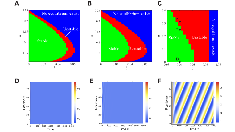
Figure 2: Parameter space analysis for reaction-diffusion-advection system (3). (A, B) Parameter maps showing stable and unstable regions without advection ($v=0$) and with advection ($v=0.3162$). (C) Parameter map showing the robustification of transport-driven instability. (D-F) Spatio-temporal profiles of the molecule $P$ for different values of parameters (see Fig. 2 (C)). The panels D and F are repeated from Fig. 1 (B) and Fig. 1 (D), respectively.

Example. We demonstrate the SDP based stability test using the reaction-diffusion-advection system (3). Let $[C_{1}^{*},C_{2}^{*}]^{T}$ be a spatially homogeneous equilibrium point of the system and consider the linearized system (4). It follows from (3) that

$$C_{1}^{*}=\frac{1}{2}(1-\sqrt{w}),\,C_{2}^{*}=\frac{a}{2(a+b)}(1+\sqrt{w})$$ (21)

is an equilibrium point, where $w:=1-4(a+b)^{2}/a$. The Jacobian linearization leads to

$$\frac{\partial}{\partial t}\begin{bmatrix}c_{1}\\ c_{2}\end{bmatrix}=\begin{bmatrix}-a-C_{2}^{*2}&-2C_{1}^{*}C_{2}^{*}\\ C_{2}^{*2}&-(a+b)+2C_{1}^{*}C_{2}^{*}\end{bmatrix}\begin{bmatrix}c_{1}\\ c_{2}\end{bmatrix}+\begin{bmatrix}d&0\\ 0&1\end{bmatrix}\begin{bmatrix}\nabla^{2}c_{1}\\ \nabla^{2}c_{2}\end{bmatrix}+\begin{bmatrix}v_{1}&0\\ 0&v_{2}\end{bmatrix}\begin{bmatrix}\nabla c_{1}\\ \nabla c_{2}\end{bmatrix}.$$ (22)

To analyze the stability of the equilibrium point, we substitute the parameters into (7) and compute the polynomials $\varphi_{\rm Re}(\zeta,s)$ and $\varphi_{\rm Im}(\zeta,s)$, and define the Sylvester matrix $S$ defined in (9).

Here we first consider the parameter values used in Fig. 1(B), where $(b,v_{1},v_{2})=(0.040,0,0)$ (see Method section for the other parameters). The corresponding polynomials $\Delta_{i}(\zeta)~{}(i=1,2)$ are then obtained as

$$\Delta_{1}(\zeta)=7\zeta^{2}+0.184,$$ (23)

$$\Delta_{2}(\zeta)=294\zeta^{8}-0.0382\zeta^{6}+0.192\zeta^{4}+0.0315\zeta^{2}+0.000555.$$ (24)

Hurwitz’s stability condition implies that the equilibrium $[C_{1}^{*},C_{2}^{*}]$ is stable if and only if $\Delta_{1}(\zeta)>0$ and $\Delta_{2}(\zeta)>0$ for all $\zeta\in\mathbb{R}$. It is obvious that $\Delta_{1}(\zeta)>0$, but the sign of $\Delta_{2}(\zeta)$ needs further examination. Thus, we use the condition (ii) of Proposition 1 to derive conditions for non-negativity of $\Delta_{1}(\zeta)$ and $\Delta_{2}(\zeta)$. The positivity of $\Delta_{1}(\zeta)$ can be easily confirmed since $\Delta_{1}(\zeta)={\bm{z}}_{1}^{T}M_{1}{\bm{z}}_{1}$ with $M_{1}=\mathrm{diag}(0.184,7)\succ O$ and ${\bm{z}}_{1}=[1,\zeta]^{T}$. On the other hand, $\Delta_{2}(\zeta)$ is expressed as $\Delta_{2}(\zeta)={\bm{z}}_{2}^{T}M_{2}{\bm{z}}_{2}$ with monomials ${\bm{z}}_{2}:=[1,\zeta,\zeta^{2},\zeta^{3},\zeta^{4}]^{T}$ and $M_{2}=\mathrm{diag}(0.000555,0.0315,\allowbreak 0.192,-0.0382,294)$. Thus, we examine the existence of a matrix $N_{2}$ such that $M_{2}+N_{2}\succ O$ and $\sum_{(j,k)\in\Theta_{\ell}}\nu_{jk}^{(2)}=0~{}(\ell=2,3,\cdots,10)$ by solving the feasibility problem of the optimization program. The optimization solver yields

$$N_{2}=\begin{bmatrix}0&0&-0.0264&0&0.0710\\ 0&0.0528&0&-1.3655&0.0012\\ -0.0264&0&2.5889&-0.0012&-16.797\\ 0&-1.3655&-0.0012&33.595&0\\ 0.0710&0.0012&-16.797&0&0\end{bmatrix}$$ (25)

which indeed satisfies $M_{2}+N_{2}\succeq O$ and $\sum_{(j,k)\in\Theta_{\ell}}\nu_{jk}^{(2)}=0~{}(\ell=2,3,\cdots,10)$. This implies that $\Delta_{2}(\zeta)={\bm{z}}_{2}^{T}(M_{2}+N_{2}){\bm{z}}_{2}={\bm{z}}_{2}^{T}M_{2}{\bm{z}}\geq 0$ for all $\zeta\in\mathbb{R}$. Thus, the equilibrium point is locally stable, and the concentrations $[C_{1},C_{2}]^{T}$ converge to the equilibrium when they are perturbed in the vicinity of $[C_{1}^{*},C_{2}^{*}]$ (Fig. 1(B)).

To see an example of an unstable case, we next consider the parameter sets used in Fig. 1(C), that is, $(b,v_{1},v_{2})=(0.055,0,0)$ (see Method section for the other parameters). In this case,

$$\Delta_{1}(\zeta)=7\zeta^{2}+0.0679,$$ (26)

$$\Delta_{2}(\zeta)=294\zeta^{8}-19.141\zeta^{6}-0.0999\zeta^{4}+0.0045\zeta^{2}+0.000033.$$ (27)

Thus, the sign of $\Delta_{2}(\zeta)$ determines the stability of the equilibrium point. The SDP solver returns “infeasible”, implying that there is no $N_{2}$ satisfying the conditions (ii) in Proposition 1. This means that there exists a spatial frequency $\zeta$ for which the characteristic polynomial $\varphi(\zeta,s)=0$ has a root in the right-half complex plane. Thus, the system (6) is unstable for the frequency $\zeta$. In particular, the destabilization occurs for some non-zero spatial frequency $\zeta$ since $\Delta_{1}(\zeta)>0$ and $\Delta_{2}(\zeta)>0$ when $\zeta=0$. This observation is consistent with the simulation result in Fig. 1(C) in that the steady state solution converges to the spatial periodic oscillations with some non-negative frequency.

Using the SDP based stability test, we further investigate how the advective flow affects the formation of spatial patterns in the reaction system (3). Specifically, we first characterize the parameter space that induces transport-driven instability with and without flow (Fig. 2 (A) and (B), respectively). In Fig. 2(B), the flow rates of $P$ and $Q$ were set $(v_{1},v_{2})=(0.3162d,0.3162)=(1.897,0.3162)$, respectively. The difference of the flow rate is due to the Stokes-Einstein relation, where the difference of the molecular size results in the diffusion and advection rates. Figures 2(A) and (B) illustrate that the advective flow broadens the parameter region for instability, implying that the formation of periodic patterns becomes more robust when there is advective flow in the system.

To further analyze the relation between the velocity of the flow and the parameter region for transport-driven instability, we define the flow rate as $(v_{1},v_{2})=(dv,v)$ and vary $v$ between 0 and 0.3162. It should be noted that $v$ is the flow rate of $Q$ and is proportional to the velocity of the constant flow in the reactor (see Fig. 1(A)). Fig. 2(C) illustrates the parameter region for transport-driven instability for different values of $v$, where $v=0$ means that the transportation of the molecules is exclusively due to passive diffusion. The result suggests that the transport-driven instability is induced by advective flow once the speed of the flow reaches a threshold. In particular, the instability region increases almost linearly with the speed of the flow and becomes almost twice as large as the diffusion only case when $v=0.40$. The spatio-temporal simulations of the reaction-diffusion-advection system show that periodic pattern formation does occur by increasing the speed of advection (Fig. 2(D-F)). Although the link between diffusion-driven instability and biological pattern formation is often criticized due to the lack of robustness, these results suggest that the advective transportation of molecules could compensate for the fragility of the diffusion-driven pattern formation.

5 Pattern formation with specified spatial profiles

In the design and analysis of reaction-diffusion-advection systems, we are often interested in the shape of spatial patterns, which is roughly determined by the spatial frequency, or the characteristic wavelength, of the spatial oscillations. This requires identification of the destabilizing frequency, that is, the frequency $\zeta$ that makes the polynomials $\Delta_{i}(\zeta)$ negative. In what follows, we extend Proposition 1 to enable local stability analysis of reaction-diffusion-advection systems for a specified range of spatial frequency $\mathcal{I}\subset\mathbb{R}$. Using the extended theorem, we can specify a range of spatial frequency $\mathcal{I}$ that destabilizes the reaction-diffusion-advection system. This facilitates the analysis and design of the spatial profiles of transport-driven patterns.

According to the Hurwitz condition presented in Section 4, the reaction-diffusion-advection system (4) is stable for a given range of spatial frequency $\mathcal{I}\in\mathbb{R}$ if and only if the polynomials $\Delta_{i}(\zeta)~{}(i=1,2,\cdots,n)$ is positive for all $\zeta\in\mathcal{I}$. To check the sign of $\Delta_{i}(\zeta)$ for a given rage $\mathcal{I}$, we again introduce a set of linear matrix inequalities that is amenable to semidefinite programming.

Proposition 2. Let $\mathcal{I}$ denote an open interval on real numbers, i.e., $\mathcal{I}\subset\mathbb{R}$. The following (i)–(iii) are equivalent.

• $\Delta_{i}(\zeta)\geq 0$ for all $\zeta\in\mathcal{I}$ and $i=1,2,\cdots,n$.

• There exist polynomials $f(\zeta)$ and $g(\zeta)$ such that $f(\zeta)\geq 0$ and $g(\zeta)\geq 0$ for all $\zeta\in\mathbb{R}$, and $\Delta_{i}(\zeta)=f(\zeta)+h(\zeta)g(\zeta)$, where

  $$h(\zeta):=\begin{cases}-(\zeta-\underline{\zeta})(\zeta-\overline{\zeta})&{\rm when~{}}\mathcal{I}=[\underline{\zeta},\overline{\zeta}]\\ \zeta-\underline{\zeta}&{\rm when~{}}\mathcal{I}:=[\underline{\zeta},\infty)\\ -\zeta+\overline{\zeta}&{\rm when~{}}\mathcal{I}:=(-\infty,\overline{\zeta}]\end{cases}.$$ (28)

• The following conditions are satisfied.

  • In the case of a finite interval $\mathcal{I}:=[\underline{\zeta},\overline{\zeta}]$, define $\delta_{\ell}^{(i)}$ as the coefficients of the polynomial

    $$\Delta_{i}\left(\frac{(\overline{\zeta}-\underline{\zeta})\zeta+(\overline{\zeta}+\underline{\zeta})}{2}\right)=\sum_{\ell}\delta_{\ell}^{(i)}\zeta^{\ell}.~{}~{}(i=1,2,\cdots,n)$$ (29)

    Then, there exists $K_{i}\in\mathbb{R}^{(\ell_{i}+1)\times(\ell_{i}+1)}$ and $L_{i}\in\mathbb{R}^{\ell_{i}\times\ell_{i}}$ such that

    $$K_{i}\succeq O,~{}~{}L_{i}\succeq O,$$ (30)

    $$\delta_{\ell}^{(i)}=\sum_{(j,k)\in\Theta_{\ell+2}}(\kappa_{jk}^{(i)}+\lambda_{jk}^{(i)})-\sum_{(j,k)\in\Theta_{\ell}}\lambda_{jk}^{(i)},$$ (31)

    where $\ell_{i}:=\lceil\mathrm{deg}(\Delta_{i}(\zeta))/2\rceil$, and $\kappa_{jk}^{(i)}$ and $\lambda_{jk}^{(i)}$ represent the $(j,k)$-th entry of the matrices $K_{i}$ and $L_{i}$, respectively. $\Theta_{\ell}$ is defined in Proposition 1.

  • In the case of a semi-infinite interval $\mathcal{I}:=[\underline{\zeta},\infty)$, define $\delta_{\ell}^{(i)}$ as the coefficients of the polynomial

    $$\Delta_{i}\left(\zeta+\underline{\zeta}\right)=\sum_{\ell}\delta_{\ell}^{(i)}\zeta^{\ell}.~{}~{}(i=1,2,\cdots,n),$$ (32)

    or in the case of $\mathcal{I}:=(-\infty,\overline{\zeta}]$, define $\delta_{\ell}^{(i)}$ as

    $$\Delta_{i}\left(-\zeta+\overline{\zeta}\right)=\sum_{\ell}\delta_{\ell}^{(i)}\zeta^{\ell}.~{}~{}(i=1,2,\cdots,n).$$ (33)

    Then, there exists $K_{i}\in\mathbb{R}^{(\ell_{i}+1)\times(\ell_{i}+1)}$ and a matrix $L_{i}$ such that

    $$K_{i}\succeq O,~{}~{}L_{i}\succeq O,$$ (34)

    $$\delta_{\ell}^{(i)}=\sum_{(j,k)\in\Theta_{\ell+2}}\kappa_{jk}^{(i)}+\sum_{(j,k)\in\Theta_{\ell+1}}\lambda_{jk}^{(i)},$$ (35)

    where $\ell_{i}:=\lceil\mathrm{deg}(\Delta_{i}(\zeta))/2\rceil$, and $\kappa_{jk}^{(i)}$ and $\lambda_{jk}^{(i)}$ represent the $(j,k)$-th entry of the matrices $K_{i}$ and $L_{i}$, respectively. The size of $L_{i}$ is $\ell_{i}+1$ by $\ell_{i}+1$ when $\mathrm{deg}(\Delta_{i}(\zeta))$ is odd, and $\ell_{i}$ by $\ell_{i}$ when $\mathrm{deg}(\Delta_{i}(\zeta))$ is even. $\Theta_{\ell}$ is defined in Proposition 1.

It should be noted that $\Theta_{\ell}$ is an empty set for $\ell=0,1$. Similar to Proposition 1, the basic idea is to explore the SOS decomposition of $\Delta_{i}(\zeta)$ to guarantee its non-negativity on the interval $\mathcal{I}$ (see Supplementary Information for the proof). This problem essentially boils down to finding $f(\zeta)$ and $g(\zeta)$ in the condition (ii). In the condition (iii) of Proposition 2, we convert the condition (ii) into the form of matrix inequalities by using the change of variable. That is, the interval $\mathcal{I}$ is converted into $[-1,1]$ and $[0,\infty)$. This leads to the simple LMI based formulation (30), (31), (34) and (35), where the existence of the matrices $K_{i}$ and $L_{i}$ is equivalent to the existence of non-negative polynomials $f(\zeta):={\bm{z}}_{i}^{T}K_{i}{\bm{z}}$ and $g(\zeta):={\bm{z}}_{i}^{T}L_{i}{\bm{z}}$ such that $\Delta_{i}(\zeta)=f(\zeta)+h(\zeta)g(\zeta)$ with $h(\zeta)=-(\zeta-1)(\zeta+1)$ for the finite interval and $h(\zeta)=\zeta$ for the infinite interval case. Since the existence problem of the matrices $K_{i}$ and $L_{i}$ can be implemented as a feasibility problem of a semidefinite program, it is possible to efficiently explore the matrices satisfying the constraints using existing solvers.

The condition (ii) of Proposition 2 enables identification of the stable and unstable spatial frequency of the reaction-diffusion-advection system. This is particularly helpful to find the parameter space of the reaction that leads to the formation of prespecified spatial patterns as demonstrated in the next example.

Remark 3.  When multi-dimensional space $\Omega$ is considered, the variable $\zeta$ in Proposition 2 is equal to the sum of the spatial frequency $\bar{\zeta}=\sum_{i=1}^{m}\zeta_{i}$ as shown in Remark 2. Thus, there can be multiple different combinations of frequency $\zeta_{i}~{}(i=1,2,\cdots,m)$ for a given destabilizing $\zeta$. This means that the growth rate of frequency components $\tilde{{\bm{c}}}({\bm{\zeta}},t)$ are equal between all combinations of $\zeta_{i}$ that sums to $\zeta$. Therefore, any of these frequency components could appear as the resulting spatial pattern depending on the initial perturbation to the homogeneous steady state $\bar{\bm{C}}$.

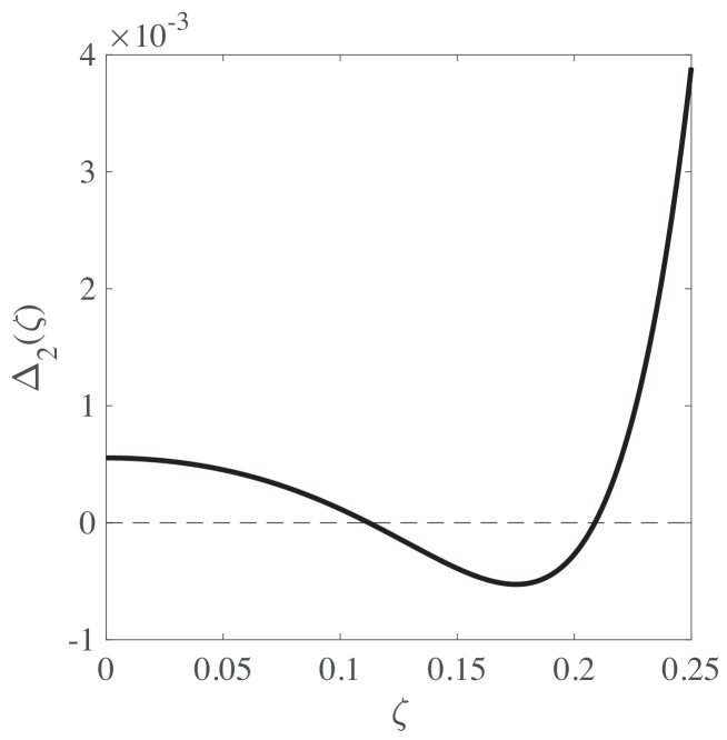
Figure 3: Value of $\Delta_{2}(\zeta)$. The reaction-diffusion-advection system is destabilized at the spatial frequency $\zeta$ satisfying $\Delta_{2}(\zeta)<0$.

Example. We consider the reaction-diffusion-advection system (3) and its linearized model (22). Let the parameters $a,b$ and $d$ be set as $(a,b,d)=(0.06,0.04,6.0)$ and $v=0.3162$, with which the equilibrium is unstable as illustrated in Fig. 2C (marked as “F”). As have already seen in the previous section, the matrix inequalities in Proposition 1(ii) are infeasible since $\Delta_{2}(\zeta)$ in (24) is negative for some $\zeta\in\mathbb{R}$. This implies that the equilibrium point of the reaction-diffusion-advection system is locally unstable, leading to the formation of the spatial pattern in Fig. 2F. To further analyze, we investigate the value of $\Delta_{2}(\zeta)$ as shown in Fig. 3. The figure implies that the reaction-diffusion-advection system is destabilized around $0.12\leq\zeta\leq 0.2$, whose wavelength corresponds to $31.4\leq 2\pi/\zeta\leq 48.3$. We observe that the wavelength of the periodic spatial pattern in Fig. 2F agrees with the destabilizing frequency.

Proposition 2 enables optimization-based analysis of the stabilizing/destabilizing frequency $\zeta$ without actually computing $\Delta_{i}(\zeta)$ unlike Fig. 3. As an example, we solve SDP with the condition (ii) in Proposition 2 by setting $\mathcal{I}=[0,0.1]$. Since $\Delta_{2}(\zeta)$ is positive on $\mathcal{I}$, the SDP is feasible and the solver finds

$$K_{2}=10^{-4}\times\begin{bmatrix}2.6498&0.5060&-11.327&-0.7936&9.7421\\ 0.5060&9.7828&-8.9253&-12.081&10.089\\ -11.327&-8.9253&79.539&11.580&-76.375\\ -0.7936&-12.081&11.580&15.730&-13.547\\ 9.7421&10.089&-76.375&-13.547&75.743\end{bmatrix}\succeq O,$$

$$L_{2}=10^{-4}\times\begin{bmatrix}1.8741&-1.5595&-4.2902&3.3575\\ -1.5595&22.153&4.7537&-38.461\\ -4.2902&4.7537&15.638&-13.547\\ 3.3575&-38.461&-13.547&75.743\end{bmatrix}\succeq O,$$

which verifies non-negativity of $\Delta_{2}(\zeta)$ for $0\leq\zeta\leq 0.1$. Similarly, for $\mathcal{I}=[0.25,\infty)$, the solver finds

$$K_{2}=\begin{bmatrix}0.0039&-0.1259&0.1373&0.1207&0.0830\\ -0.1259&8.2473&-22.293&-12.915&-10.193\\ 0.1373&-22.293&139.67&52.697&75.458\\ 0.1207&-12.915&52.697&264.83&166.16\\ 0.0830&-10.193&75.458&166.16&294.00\end{bmatrix}\succeq O,$$

$$L_{2}=\begin{bmatrix}0.4259&-2.9496&1.0891&0.9705\\ -2.9496&62.322&-11.063&12.481\\ 1.0891&-11.063&169.72&56.854\\ 0.9705&12.481&56.854&255.68\end{bmatrix}\succeq O.$$

On the other hand, the solver certifies that there is no $K_{i}$ and $L_{i}$ that satisfies conditions (ii) in Proposition 2 when $0.1<\zeta<0.25$. These results imply that $\Delta_{2}(\zeta)$ is positive for $\zeta\in[0,0.1]$ and $\zeta\in[0.25,\infty)$ and is negative for some $\zeta\in(0.1,0.25)$. Thus, the destabilizing frequency is identified as $0.1<\zeta<0.25$ without explicitly computing the value of $\Delta_{2}(\zeta)$. The SDP feasibility test introduced above allows the identification of the interval of destabilizing frequency. Using this feature, it is possible to further narrow down the parameter sets for diffusion/advection-driven instability (Fig. 2(A-C)) with the additional constraints of the wavelength of spatial patterns.

When there is a single connected interval of destabilizing frequency $\mathcal{I}$, we can also use a bisection-type algorithm to precisely estimate the destabilizing frequency. Specifically, we first solve the SOS program in Proposition 2 for some initial interval $[0,\underline{\zeta}]$ with sufficiently large $\underline{\zeta}$, and iteratively divide $\underline{\zeta}$ into a half until the SOS program in Proposition 2 returns a feasible solution. Once we find a frequency that gives a feasible solution, say $\zeta_{*}$, the lower bound of the destabilizing frequency is between $\zeta_{*}$ and $2\zeta_{*}$. Thus, we further solve the SOS program by setting $\underline{\zeta}=1.5\zeta_{*}$ and divide the domain into a half until it becomes small enough, which converges to the lower bound of the destabilizing frequency. The upper bound of the destabilizing frequency can be found by essentially the same idea, where we initially solve the SOS program in Proposition 2 for $[\overline{\zeta},\infty)$ with sufficiently small $\overline{\zeta}$, and iteratively narrow the domain by $[2\overline{\zeta},\infty)$. It should, however, be noted that this bisection-type algorithm gives only the upper and lower bounds of destabilizing frequency when there are multiple destabilizing frequency intervals. For example, $\zeta_{1}$ and $\zeta_{4}$ are obtained when there are two disconnected intervals of destabilizing frequency $\mathcal{I}_{1}=(\zeta_{1},\zeta_{2})$ and $\mathcal{I}_{2}=(\zeta_{3},\zeta_{4})$ with $\zeta_{2}<\zeta_{3}$.

6 Conclusion and Discussion

Self-organizing phenomena in spatially interacting chemical systems have been studied in biology and chemistry for a long time due to its link with biological developmental process. In microbiology, it is known that culture conditions may affect the spatial profile of bacterial colonies, and its link with reaction-diffusion systems have been extensively studied (see Chapter 11 of [2] for example). In developmental biology, experimental works revealed that spatio-temporal molecular patterning in embryos affects morphology, the structure of organisms [3, 40, 41]. This motivates spatio-temporal control of morphogen concentrations in tissue engineering [42]. In addition to the biological applications, there are potential engineering applications of molecular based communications, where spatially dispersed micro and nano-scale systems communicate with each other by small diffusible molecules [43]. Therefore, understanding the dynamics of transport-driven pattern formation will not only contribute to biological science but also helps open up new engineering applications.

This paper has proposed a novel computational approach to analyzing the local stability/instability of reaction-diffusion-advection systems. The proposed algebraic conditions in Propositions 1 and 2 bypass the iterative stability analysis of individual Fourier components and provide a route toward the direct characterization of the local behavior by a single run of mathematical optimization, speeding the analysis and synthesis of self-organizing chemical systems in biology and chemistry. The condition in Proposition 2 further allows the computation of the destabilizing spatial frequency. This helps detailed quantitative analysis of the spatio-temporal profile of the self-organizing chemical concentrations. We have numerically illustrated the optimization-based analysis process using the auto-catalytic reaction model with diffusion and advection.

From a theoretical viewpoint, our development hinges upon the sum-of-squares (SOS) optimization technique [31] to prove non-negativity of $\Delta_{i}(\zeta)$, which implies stability of the reaction-diffusion-advection systems. In the last decade, the SOS optimization was extensively studied in control engineering community to analyze the stability of nonlinear dynamical systems. Software packages were developed to facilitate the implementation of SOS optimization programs [44]. In general, the existence of SOS decomposition of a polynomial implies non-negativity, but the converse is not necessarily the case. In other words, not all non-negative polynomials can be represented as a sum of squares (see [31] for example). In our theoretical development, however, we have used the fact that the polynomial inequalities associated with the stability analysis are univariate, in which case there always exists an SOS decomposition if the polynomial is non-negative, leading to not only the sufficient but also the necessary condition for the stability of reaction-diffusion-advection systems. This is particularly useful for the study of transport-driven pattern formation since the condition can provide rigorous instability certificate of the reaction-diffusion-advection systems. It is also worth mentioning that the polynomial inequality conditions $\Delta_{i}(\zeta)\geq 0~{}(i=1,2,\cdots,n)$ are univariate even for multi-dimensional reaction-diffusion-advection systems as discussed in Remark 2. This is attractive from a viewpoint of computational burden since, in general, the size of the matrices involved in the SOS programs such as $M_{i},N_{i},K_{i}$ and $L_{i}$ grow in a combinatorial fashion with the number of variables and the degrees of polynomials, which is one of actively studied issues in recent years [45, 46, 47]. A limitation of the proposed approach is that it can only verify local properties around a given equilibrium point due to the linearization, and thus, it cannot rigorously guarantee the emergence of inhomogeneous spatial patterns in nonlinear reaction-diffusion-advection systems. To overcome this issue, an alternative approach would be to use Lyapunov’s approach to obtain sufficient conditions for global stability [27, 28, 29, 30].

A major criticism about Turing’s diffusion-driven instability is that the parameter space for the instability is too small to achieve even in engineered chemical systems although spatial pattern formation is quite a common phenomenon in biology. Recent theoretical works, on the other hand, presented that stochastic intrinsic noise of chemical reactions in biological cells enhances diffusion-driven instability, resulting in the increase of the instability parameter regime [48, 49, 50, 51]. Our transport-driven instability analysis in Fig. 2(A)-(C) suggests that advective flow is another factor that broadens the parameter space for transport-driven instability. In fact, Fig. 2F shows that the originally stable reaction-diffusion system (Fig. 2D) exhibits spatially inhomogeneous patterns by adding the flow. These results imply that the robustness of self-organization in nature could be guaranteed by circulatory systems in addition to intrinsic noise.

The idea of flow-driven instability was previously presented in [21, 52, 53, 54], where periodic spatial patterns were observed due to the destabilizing effect of advection. The theoretical prediction was also verified with engineered chemical and biological systems [22, 55]. Unlike the model (3) in this paper, the previous analyses were limited for systems where only one molecule could diffuse and flow while other molecules were immobilized. This assumption can be easily relaxed with the proposed stability analysis method as it is capable of dealing with arbitrarily many diffusing and flowing molecules in principle despite the complex eigenvalues of the advection operator. Although this paper has only shown a simple reaction example to focus on the verification and demonstration of the theoretical development, it will be helpful to examine more biologically relevant models, in future, to understand the underlying mechanisms of the flow-driven robustification of the spatial pattern formation. The authors also envision that there are potential extensions of the proposed SOS programs to robust stability analysis and (reaction) design problems, given that these topics are actively studied using SOS programs in control systems community [56].

Method

The spatio-temporal dynamics in Fig. 1(B)-(D) and Fig. 2(D)-(F) were simulated with the periodic boundary condition using Wolfram Mathematica 11.0.1.0 on macOS 10.12.6. These colormaps illustrate the concentration of $P$, or $C_{1}(x,t)$. In all simulations, $a=0.06$ and $d=6.0$ were used. The spatial length was $L=30\pi$. Figure 2(D) and (F) are repeated from Fig. 1(B) and (D), respectively, for the clarity of presentation. For Fig. 2(E), the parameters were set $a=0.06,b=0.04,d=6.0,v_{1}=1.518,v_{2}=0.2530$. For all spatio-temporal simulations, the initial values were set $C_{1}(x,0)=0.5+0.0025\sum_{k=1}^{20}\{\cos(2k\pi x/L)+\sin(2k\pi x/L)\}$ and $C_{2}(x,0)=0.2+0.0025\sum_{k=1}^{20}\{\cos(2k\pi x/L)+\sin(2k\pi x/L)\}$.

The semidefinite programs were run with SeDuMi 1.3 [57] and YALMIP toolbox [58] on MATLAB 2016b.

Data, codes and materials

The program codes used in this study are available at GitHub (https://github.com/hori-group/SDP_for_flow-driven_stability_analysis)

Competing interests

The authors have no competing interests.

Authors’ contributions

Y.H. conceived of and designed the study. Both authors performed the mathematical derivation and implemented the computational codes for optimization and simulations. Both authors drafted the manuscript and gave final approval for publication.

Funding

This work was supported in part by JSPS KAKENHI Grant Number JP18H01464 and 15J09841.

References

- [1] Koch AJ, Meinhardt H. Biological pattern formation: from basic mechanisms to complex structures. Reviews of Modern Physics. 1994;66(4):1481–1507.
- [2] Murray JD. Mathematical Biology II. 3rd ed. Springer; 2003.
- [3] Kondo S, Miura T. Reaction-diffusion model as a framework for understanding biological pattern formation. Science. 2010;329(5999):1616–1620.
- [4] Hu Z, Lutkenhaus J. Topological regulation of cell division in Escherichia coli involves rapid pole to pole oscillation of the division inhibitor MinC under the control of MinD and MinE. Molecular Microbiology. 1999;34(1):82–90.
- [5] Meinhardt H, de Boer PAJ. Pattern formation in Escherichia coli: A model for the pole-to-pole oscillations of Min proteins and the localization of the division site. Proceedings of National Academy of Sciences of the United States of America. 2001;98(25):14202–14207.
- [6] Lutkenhaus J. Assembly Dynamics of the Bacterial MinCDE System and Spatial Regulation of the Z Ring. Annual Review of Biochemistry. 2007;76:539–562.
- [7] Rudner DZ, Losick R. Protein subcellular localization in bacteria. Cold Spring Harbor Perspectives in Biology. 2010;2:a000307.
- [8] Vecchiarelli AG, Li M, Mizuuchi M, Hwang LC, Seol Y, Neuman KC, et al. Membrane-bound MinDE complex acts as a toggle switch that drives Min oscillation coupled to cytoplasmic depletion of MinD. Proceedings of National Academy of Sciences of the United States of America. 2016;113(11):E1479–E1488.
- [9] Castets VV, Dulos E, Boissonade J, Kepper PD. Experimental evidence of a sustained standing Turing-type nonequilibrium chemical pattern. Physical Review Letters. 1990;64(24):2953–2956.
- [10] Ouyang Q, Swinney HL. Transition from a uniform state to hexagonal and striped Turing patterns. Nature. 1991;352:610–612.
- [11] You L, III RSC, Weiss R, Arnold FH. Programmed population control by cell-cell communication and regulated killing. Nature. 2004;428(6985):868–871.
- [12] Basu S, Gerchman Y, Collins CH, Arnold FH, Weiss R. A synthetic multicellular system for programmed pattern formation. Nature. 2005;434(7037):1130–1134.
- [13] Liu C, Fu X, Liu L, Ren X, Chau CKL, Li S, et al. Sequential establishment of stripe patterns in an expanding cell population. Science. 2011;334(6053):238–241.
- [14] Moon TS, Lou C, Tamsir A, Stanton BC, Voigt CA. Genetic programs constructed from layered logic gates in single cells. Nature. 2012;491(7423):249–253.
- [15] Tamsir A, Tabor JJ, Voigt CA. Robust multicellular computing using genetically encoded NOR gates and chemical ‘wires’. Nature. 2011;469(7329):212–215.
- [16] Danino T, Mondragón-Palomino O, Tsimring L, Hasty J. A synchronized quorum of genetic clocks. Nature. 2010;463(7279):326–330.
- [17] Din MO, Danino T, Prindle A, Skalak M, Selimkhanov J, Allen K, et al. Synchronized cycles of bacterial lysis for in vivo delivery. 536. 2016;536:81–85.
- [18] Scott SR, Din MO, Bittihn P, Xiong L, Tsimring LS, Hasty J. A stabilized microbial ecosystem of self-limiting bacteria using synthetic quorum-regulated lysis. Nature Microbiology. 2017;2(12):17083.
- [19] Baumgart L, Mather W, Hasty J. Synchronized DNA cycling across a bacterial population. Nature genetics. 2017;49(8):1282–1285.
- [20] Turing AM. The chemical basis of morphogenesis. Philosophicals Transactions of the Royal Society of London B. 1952;237(641):37–72.
- [21] Rovinsky AB, Menzinger M. Chemical instability induced by a differential flow. Physical Review Letters. 1992;69(8):1193–1196.
- [22] Rovinsky AB, Menzinger M. Self-organization induced by the differential flow of activator and inhibitor. Physical Review Letters. 1993;70(6):778–781.
- [23] Gierer A, Meinhardt H. A theory of biological pattern formation. Kybernetik. 1972;12(1):30–39.
- [24] Hori Y, Miyazako H, Kumagai S, Hara S. Coordinated Spatial Pattern Formation in Biomolecular Communication Networks. IEEE Transactions on Molecular, Biological, and Multi-Scale Communications. 2015;1(2):111–121.
- [25] Boyd S, Ghaoui LE, Feron E, Balakrishnan V. Linear matrix inequalities in system and control theory. Society for Industrial and Applied Mathematics; 1994.
- [26] Boyd S, Vandenberghe L. Convex Optimization. Cambridge University Press; 2008.
- [27] Jovanović MR, Arcak M, Sontag ED. A Passivity-Based Approach to Stability of Spatially Distributed Systems With a Cyclic Interconnection Structure. IEEE Transactions on Automatic Control. 2008;53:75–86. (special issue).
- [28] Arcak M. Certifying spatially uniform behavior in reaction-diffusion PDE and compartmental ODE systems. Automatica. 2011;47(6):1219–1229.
- [29] Shafi SY, Aminzare Z, Arcak M, Sontag ED. Spatial uniformity in diffusively-coupled systems using weighted L2 norm contractions. In: Proceedings of American Control Conference; 2013. p. 5639–5644.
- [30] Valmorbida G, Ahmadi M, Papachristodoulou A. Stability analysis for a class of partial differential equations via semidefinite programming. IEEE Transactions on Automatic Control. 2016;61(6):1649–1654.
- [31] Parrilo PA. Semidefinite programming relaxations for semialgebraic problems. Mathematical Programming. 2003;96(2):293–320.
- [32] Gray P, Scott SK. Autocatalytic reactions in the isothermal continuous stirred tank reactor. Chemical Engineering Science. 1984;39(6):1087–1097.
- [33] Pearson JE. Complex patterns in a simple system. Science. 1993;261(5118):189–192.
- [34] Strauss WA. Partial differential equations: an introduction. 2nd ed. John Wiley & Sons, Inc.; 2007.
- [35] Bamforth JR, Merkin JH, Scott SK, Tóth R, Gáspár V. Flow-distributed oscillation patterns in the Oregonator model. Physical Chemistry Chemical Physics. 2001;3(8):1435–1438.
- [36] Hinrichsen D, Pritchard AJ. Mathematical Systems Theory I. 3rd ed. Springer; 2011.
- [37] Sturm JF. Using SeDuMi 1.02, a MATLAB toolbox for optimization over symmetric cones. Optimization Methods and Software. 1999;11–12:625–653.
- [38] Toh KC, Todd MJ, Tutuncu RH. SDPT3 — a Matlab software package for semidefinite programming. Optimization Methods and Software. 1999;11:545–581.
- [39] Forsgren A, Gill PE, Wright MH. Interior Methods for Nonlinear Optimization. SIAM review. 2002;44(4):525–597.
- [40] Palmeirim I, Henrique D, Ish-Horowicz D, Pourquie O. Avian hairy Gene Expression Identifies a Molecular Clock Linked to Vertebrate Segmentation and Somitogenesis. Cell. 1997;91(5):639–648.
- [41] Bessho Y, Sakata R, Komatsu S, Shiota K, Yamada S, Kageyama R. Dynamic expression and essential functions of Hes7 in somite segmentation. Genes and Development. 2001;15(20):2642–2647.
- [42] Biondi M, Ungaro F, Quaglia F, Netti PA. Controlled drug delivery in tissue engineering. Advanced Drug Delivery Reviews. 2008;60(2):229–242.
- [43] Nakano T, Suda T, Okaie Y, Moore MJ, Vasilakos AV. Molecular communication among biological nanomachines: a layered architecture and research issue. IEEE Transactions on NanoBioscience. 2014;13(3):169–197.
- [44] Papachristodoulou A, Anderson J, Valmorbida G, Prajna S, Seiler P, Parrilo PA. SOSTOOLS: Sum of squares optimization toolbox for MATLAB. http://arxiv.org/abs/1310.4716; 2013. Available from http://www.eng.ox.ac.uk/control/sostools, http://www.cds.caltech.edu/sostools and http://www.mit.edu/~parrilo/sostools.
- [45] Waki H, Kim S, Kojima M, Muramatsu M. Sums of squares and semidefinite program relaxations for polynomial optimization problems with structured sparsity. SIAM Journal on Control and Optimization. 2006;17(1):218–242.
- [46] Ahmadi AA, Majumdar A. DSOS and SDSOS optimization: more tractable alternatives to sum-of-squares and semidefinite optimization; 2017. ArXiv:1706.02586.
- [47] Weisser T, Lasserre JB, Toh KC. Sparse-BSOS: a bounded degree sos hierarchy for large scale polynomial optimization with sparsity. Mathematical Programming Computation. 2018;10(1):1–32.
- [48] Biancalani T, Fanelli D, Patti FD. Stochastic Turing patterns in the Brusselator model. Physical Review E. 2010;81(4):046215.
- [49] Butler T, Goldenfeld N. Fluctuation-driven Turing patterns. Physical Review E. 2011;84(1):011112.
- [50] Scott M, Poulin FJ, Tang H. Approximating intrinsic noise in continuous multispecies models. Proceedings of the Royal Society A. 2011;467(2127):718–737.
- [51] Hori Y, Hara S. Noise-induced spatial pattern formation in stochastic reaction-diffusion systems. In: Proceedings of the IEEE Conference on Decision and Control; 2012. p. 1053–1058.
- [52] Malchow H. Motional Instabilities in Prey-Predator Systems. Journal of Theoretical Biology. 2000;204(4):639–647.
- [53] Gholami A, Steinbock O, Zykov V, Bodenschatz E. Flow-driven instabilities during pattern formation of Dictyostelium discoideum. New Journal of Physics. 2015;17(6):063007.
- [54] Vidal-Henriquez E, Zykov V, Bodenschatz E, Gholami A. Convective instability and boundary driven oscillations in a reaction-diffusion- advection model. Chaos. 2017;27:103110.
- [55] Eckstein T, Vidal-Henriquez E, Bae A, Zykov V, Bodenschatz E, Gholami A. Influence of fast advective flows on pattern formation of Dictyostelium discoideum. PLoS ONE. 2018;13(3):e0194859.
- [56] Papachristodoulou A, Prajna S. A tutorial on sum of squares techniques for systems analysis. In: Proceedings of American Control Conference; 2005. p. 2686–2700.
- [57] Sturm JF. Using SeDuMi 1.02, a MATLAB toolbox for optimization over symmetric cones. Optimization Methods and Software. 1999;11–12:625–653.
- [58] Löfberg J. YALMIP : A Toolbox for Modeling and Optimization in MATLAB. In: In Proceedings of the CACSD Conference. Taipei, Taiwan; 2004. .