On the crack-driving force of phase-field models in linearized and finite elasticity

Abstract

The phase-field approach to fracture has been proven to be a mathematically sound and easy to implement method for computing crack propagation with arbitrary crack paths. Hereby crack growth is driven by energy minimization resulting in a variational crack-driving force. The definition of this force out of a tension-related energy functional does, however, not always agree with the established failure criteria of fracture mechanics. In this work different variational formulations for linear and finite elastic materials are discussed and ad-hoc driving forces are presented which are motivated by general fracture mechanical considerations. The superiority of the generalized approach is demonstrated by a series of numerical examples.

1 Introduction

A crack in a solid with domain $\Omega$ forms a new surface of a priori unknown size, position and evolution. In order to compute such moving boundary problems, phase-field simulations of fracture have gained enormous popularity recently, e.g., Henry and Levine (2004); Karma et al. (2001); Miehe et al. (2010); Verhoosel and de Borst (2013); Borden et al. (2012); Miehe and Schänzel (2014); Sargado et al. (2018). The basic idea behind this approach is to introduce an additional field -the phase field- which indicates the material’s state. The continuous phase field $z(\bm{x},t)$ describes the solid state by $z=0$ and the broken state by $z=1$ and evolves in space $\bm{x}\in\Omega$ and time $t\in[0,\mathcal{T}]$. Because the phase field is by definition a continuous field and the moving crack boundaries are ’smeared’ over a small but finite zone of width $l_{c}$, the phase-field fracture approach constitutes a diffuse-interface formulation.

In computational mechanics the phase-field simulations of fracture have basically started with the seminal work of Bourdin et al. (2008), who showed that the diffuse-interface formulation converges in the limit $l_{c}\to 0$ to the sharp interface model of the classical Griffith theory of brittle fracture. Since then, numerous applications and enhancements have been examined. Among others Teichtmeister et al. (2017); Bleyer and Alessi (2018) expanded the phase-field model to anisotropic brittle fracture, Ambati et al. (2015, 2016); Kuhn et al. (2016) investigated ductile fracture in more detail and Heider and Markert (2017); Ehlers and Luo (2017) address to hydraulic fracture explicitly, to name some of them.

Finite element simulations of fracture problems using the phase-field method have mainly been motivated by the fact, that a rigorous connection between the phase-field and the sharp crack approach has been proven, regarding convergence of energy, energy release and evolution as the internal length $l_{c}$ vanishes, cf. Bourdin et al. (2008); Freddi and Royer-Carfagni (2010); Negri (2013) and others. The link to Griffith’s theory of fracture is usually made by means of global minimization arguments using $\Gamma$-convergence theory for instance. Such analyses obviously presume a variational setting, like it is employed in finite element methods to determine phase-field and deformation field by energy optimization.

The propagation of a crack requires a state of tension at the crack tip. For mathematical analyses this state is typically presumed a priori, whereas for numerical simulations extra effort is needed to comply with this physical constraint. A common way to ensure a tensional state during crack growth is to split the body’s energy into a tension-related and a compressive energy functional and to optimize for the phase-field only the first. Thus, it results in a hybrid variational formulation, where the body’s displacement field is obtained from the optimum of the full energy and the phase-field is obtained from the optimum of the tension-related part of the energy. Of course, such a modification also allows for a mathematical rigorous treatment. The problem of the hybrid variational formulation is, however, the lacking connection to established theories of fracture mechanics.

The classical Griffith theory underlying the phase-field fracture approaches is a model which is valid for ideal elastic and brittle materials under tension. Its generalization, for example to ductile materials, is not covered by the original theory, just as little as the common extensions of phase-field fracture models to materials showing plastic behavior. Here we suggest to open the phase-field fracture approach to a wider range of applications by using physically motivated but not variationally determined crack-driving forces. Such driving forces do not minimize an energy potential because they are established ad-hoc, i.e. postulated from a failure criterion for brittle (or ductile) materials. In consequence, they allow to account for different types of fracture observed in the engineering practice. In this paper we show numerical examples computed with different physically motivated crack-driving forces and discuss their validity. We also show that some problems, like the compressive-split test of civil engineering, definitely require the use of a classical fracture mechanics strategy to obtain simulation results which match experimental observations.

The remaining of the paper is organized as follows: At next we will present the basic equations of the phase-field fracture approach for linear and finite elasticity in Section 2. In Section 3 the common energy splits for the linear and nonlinear models are described and different definitions of their tensile components, which establish the variational crack-driving forces, are compared. Additionally to the driving forces of the classical approach, a series of physically motivated ad-hoc driving forces are presented. Section 4 is devoted to the numerical examples. In the first part of this section we discuss various two-dimensional parametric studies, then follow two real-world problems. We show numerical simulations of a Brazilian test and a conchoidal fracture specimen and discuss different crack-driving forces of linear and nonlinear elasticity. A short summary closes the paper in Section 5.

2 The phase-field approach to fracture

Crack growth within a solid which of domain $\Omega\subset\mathbb{R}^{3}$ and with boundary $\partial\Omega\equiv\Gamma\subset\mathbb{R}^{2}$ corresponds to the creation of new boundary surfaces $\Gamma(t)$. Therefore, the total potential energy of a homogenous but cracking solid is composed of its material’s energy density $\Psi^{\text{mat}}$, and of a surface energy contribution from growing crack boundaries.

$$E=\int_{\Omega}\Psi^{\text{mat}}\,\mathrm{d}\Omega+\int_{\Gamma(t)}{\mathcal{G}}_{c}\,\mathrm{d}\Gamma$$ (1)

The material’s energy will be restricted within this investigation to an elastic free Helmholtz energy density, $\Psi^{\text{mat}}=\Psi^{e}$. The fracture-surface energy density $\mathcal{G}_{c}$ quantifies the material’s resistance to cracking; for brittle fracture it corresponds to Griffith’s critical energy release rate. Both depend on the body’s unknown displacement field $\bm{u}(\bm{x},t):\Omega\times[0,\mathcal{T}]\rightarrow\mathbb{R}^{3}$. In the course of solution $\bm{u}(\bm{x},t)$ can be found when the energy attains a minimum. Unfortunately, functional (1) cannot be optimized in general and even an time-incremental technique is challenging because of the moving boundaries $\Gamma(t)$.

In the phase-field approach to fracture, the set of evolving crack boundaries is approximated by a surface-density function $\gamma=\gamma(z(\bm{x},t))$ and

$$\int_{\Gamma(t)}\ \text{d}\Gamma\approx\int_{\Omega}\gamma(z(\bm{x},t))\ \text{d}\Omega$$ (2)

which allows to re-write the dissipative energy functional of a cracking solid and to formulate the optimization problem locally.

$$E=\int_{\Omega}\left(\Psi^{e}+{\mathcal{G}}_{c}\gamma\right)\,\mathrm{d}\Omega\ \rightarrow\ \text{ optimum}$$ (3)

The elastic energy density is a function of phase-field and displacement, $\Psi^{e}(z,\bm{u})$. By definition of the surface-density function $\gamma(z)$, the fracture energy contribution $\mathcal{G}_{c}\gamma(z)$ is only different from zero along cracks.

There are different ways to formulate the surface-density function, cf. Borden et al. (2014); Hesch et al. (2016); here we will refer only to the second-order form

$$\gamma(z,\nabla z)=\frac{1}{2l_{c}}z^{2}+\frac{l_{c}}{2}|\nabla z|^{2}\,.$$ (4)

The first term results in a jump at the crack whereas the gradient term regularizes the discontinuity; the length-scale parameter $l_{c}$ defines the width of the regularized, diffuse crack zone. Inserting the crack density function (4) in the total potential energy (3) result in the well-known Ambrosio-Tortorelli functional of continuum damage mechanics, cf. Ambrosio and Tortorelli (1990). One main difference between the phase-field model and gradient damage models is that the order parameter can be just interpreted in the limits, $z=0$ indicates the intact solid material and $z=1$ the broken state. Values $z\in(0,1)$ have no physical meaning.

2.1 Phase-field evolution equation

The minimization of potential (3) is in phase-field modeling typically restated as a gradient flow problem. This results in an evolution equation for the phase-field, $\dot{z}(\bm{x},t)=\delta_{z}\Psi$, with $\Psi$ being the entire integrand of the potential (3). For balancing the units, a mobility parameter $M$ [$\mathrm{m^{2}/N\,s}$] is introduced which can also be understood as an inverse viscosity. Collecting the driving forces and denoting their magnitude with $Y$ we may formulate the phase-field evolution as typical Allen-Cahn equation,

$$\dot{z}=MY(\bm{u},z)\,.$$ (5)

Normalizing the evolution equation gives a dimensionless effective driving force $\bar{Y}=\nicefrac{{l_{c}}}{{\mathcal{G}_{c}}}Y$,

$$\tau\dot{z}=\bar{Y}(\bm{u},z)\,,$$ (6)

where $\tau=l_{c}/(M\mathcal{G}_{c})$ is the retardation time [sec] of phase field evolution.

In the remaining of this paper we employ the normalized evolution equation (6). The corresponding driving force can be written for a general, non-variational approach as

$$\bar{Y} =\bar{Y}^{e}+l_{c}\delta\gamma\,$$ (7)

where $\bar{Y}$ is postulated as the difference of an effective crack-driving force $\bar{Y}^{e}$ and the geometrical crack resistance $l_{c}\delta\gamma$, i.e. the normalized regularizing term $\mathcal{G}_{c}\gamma$ in (3). For the variational approach the generalized driving force can be formulated as

$$\bar{Y}=\delta\bar{\Psi}=\delta\bar{\Psi}^{e}-(z+l_{c}^{2}\triangle z)$$ (8)

with $\bar{\Psi}^{e}=\nicefrac{{l_{c}}}{{{\mathcal{G}}_{c}}}\Psi^{e}(\bm{u},z)$.

In addition to that, in the cracked state the driving force has to vanish, $\bar{Y}(z=1)=0$, such that the phase-field parameter stays limited. This is symbolized by the Macaulay brackets. Now, inserting the driving force $\bar{Y}$ into eq. (6) the evolution equation can be re-written as

$$\tau\dot{z}=\langle\bar{Y}^{e}+l_{c}\delta\gamma\rangle_{+}.$$ (9)

The viscous regularization is determined by the choice of retardation time $\tau$, or, equivalently, mobility parameter $M$ in (5). If the retardation time $\tau=\nicefrac{{l_{c}}}{{M\mathcal{G}_{c}}}$ very small or the mobility is high, the phase-field changes suddenly and the effect of numerical regularization vanishes. If the mobility is too low and the retardation time too high, the phase-field evolution is suppressed and the structure stiffens artificially. Therefore, the retardation time has to be set is such a way, that the phase-field is allowed to significantly evolve within one step of time discretization. This is guaranteed, when it is in the order of magnitude of a time step, i.e.

$$\tau=O(\Delta t)$$ (10)

or $\tau\approx c\Delta t$ where a constant of $c=\nicefrac{{1}}{{10}}\dots 10$ still leads almost identical results. Translated into the mobility of eq.(5) this is $M\approx 2l_{c}/(c\Delta t\,\mathcal{G}_{c})$.

\psfrag{force}{\small{$F_{\text{max}}$ [N]}}\psfrag{displacement}[cc][cc]{\small{$\bar{u}$ [mm]}}\includegraphics[width=195.12767pt]{mobilityGc.eps}

\psfrag{force}{\small{$F_{\text{max}}$ [N]}}\psfrag{displacement}[cc][cc]{\small{$\bar{u}$ [mm]}}\includegraphics[width=195.12767pt]{mobilitySc.eps}

Figure 1: Load-displacement curves for a mode-I tension tension test computed with different relaxation times $\tau$ for an elastic energy driven crack growth (left) and for a principal stress driven crack growth (right)

Figure 1 shows load-displacement curves for a mode-I tension test calculated with different values of $\tau$. The specific setup of the test is described in Sect. 4.1.5, the details of the crack propagation criteria are discussed below. Nonetheless we see, that for both crack-driving forces a high retardation time results in a higher maximum loading before crack growth and, thus, an overrated load carrying capacity of the structure.

Please note that the effect of viscous regularization holds for the phase-field evolution in general. It is independent of the criterium of crack evolution, i.e. the specific crack-driving force on the right hand side of eq. (6). The strategy of Miehe et al. (2015b, a), where an extra mobility parameter was introduced for the complementary energy as crack-driving force, cannot be confirmed here.

2.2 Linear elasticity

In classical linear elasticity the strain-energy function is defined as a function of displacement $\bm{u}$,

$$\Psi^{e}=\frac{1}{2}\bm{\epsilon}(\bm{u}):\mathbb{C}:\bm{\epsilon}(\bm{u}),$$ (11)

where $\bm{\epsilon}(\bm{u})=\operatorname{sym}(\nabla\bm{u})$ is the strain tensor and $\mathbb{C}$ is the Hookean material tensor which, for an isotropic material with Lamé constants $\lambda$ and $\mu$, has the components $C_{ijkl}=\lambda\delta_{ij}\delta_{kl}+\mu\left(\delta_{ik}\delta_{jl}+\delta_{il}\delta_{jk}\right)$. Typically, we formulate (11) with the decomposition of the strain tensor into volumetric and deviatoric components, $\bm{\epsilon}=\nicefrac{{1}}{{3}}\operatorname{tr}\bm{\epsilon}\bm{I}+\operatorname{dev}\bm{\epsilon}$,

$$\Psi^{e}=\frac{1}{2}\lambda\left(\operatorname{tr}\bm{\epsilon}\right)^{2}+\mu\left|\bm{\epsilon}\right|^{2}=\frac{1}{2}K\left(\operatorname{tr}\bm{\epsilon}\right)^{2}+\mu\left|\operatorname{dev}\bm{\epsilon}\right|^{2},$$ (12)

where $K=\lambda+\nicefrac{{2}}{{3}}\mu$ is the bulk modulus and $|\bullet|^{2}$ denotes the natural Frobenius norm. The elastic stresses are conjugate to the strains.

$$\bm{\sigma}=\frac{\partial\Psi^{e}}{\partial\bm{\epsilon}}\stackrel{{\scriptstyle\phantom{\text{isotrop}}}}{{=}} \mathbb{C}:\epsilon(\bm{u})$$ (13)

$$\stackrel{{\scriptstyle\text{isotrop}}}{{=}} \lambda\operatorname{tr}\bm{\epsilon}\bm{I}+2\mu\bm{\epsilon}=K\operatorname{tr}\bm{\epsilon}\bm{I}+2\mu\operatorname{dev}\bm{\epsilon}\,.$$

2.3 Finite elasticity

The general concept of Griffith’s critical energy release rate and the corresponding potential energy (3) is limited to brittle fracture but does not presume small deformations. The approach is also valid in the finite deformation regime with deformation mapping $\mbox{\boldmath$\chi$}(\bm{X},t):\Omega\times[0,\mathcal{T}]\rightarrow\mathbb{R}^{3}$ and $\bm{X}+\bm{u}(\bm{x},t)=\mbox{\boldmath$\chi$}(\bm{X},t)$; the fields in capitals refer to the initial configuration. We define the deformation gradient and its determinant,

$$\bm{F}=\nabla_{\mbox{\scriptsize$\mathrm{\bm{X}}$}}\hskip 2.56073pt{\mbox{\boldmath$\chi$}}\quad\text{ and }\quad J=\det\bm{F}\,,$$ (14)

and also the right Cauchy-Green stress tensor $\bm{C}$ and its isochoric part,

$$\bm{C}=\bm{F}^{T}\bm{F}\quad\text{ and }\quad\bar{\bm{C}}=J^{2/3}\bar{\bm{C}}\,.$$ (15)

To formulate the elastic strain energy functions of different material models it is useful to work with the well-known principal invariants of the right Cauchy-Green deformation tensor for an isotropic elastic material, namely $I_{1}=\operatorname{tr}(\bm{C})$, $I_{2}=\operatorname{tr}(\operatorname{cof}\bm{C})$ and $I_{3}=\operatorname{det}\bm{C}$. They can be also be expressed with the principal eigenvalues $\lambda_{a}$, $a\in\{1,2,3\}$, e.g. $I_{1}=\lambda_{1}^{2}+\lambda_{2}^{2}+\lambda_{3}^{2}$.

Then, we define the elastic strain energy $\Psi^{e}=\Psi^{e}(I_{1},I_{2},I_{3})$, where an additional dependence on the phase-field enters in the presence of cracks. Exemplarily we state here the strain energy density function of a classical Mooney-Rivlin material,

$$\Psi^{e}=\frac{\mu}{2}[(I_{1}-3+k(I_{2}-3)]+\frac{K}{2}(J-1)^{2}$$ (16)

with initial shear modulus $\mu$, second shear modulus $\mu_{2}$ and $k=\mu_{2}/\mu$; $K$ is again the bulk modulus. Constitutive relation (16) implicitly requires an a priori incompressible material. For numerical computations (nearly) incompressible material behavior is commonly modeled by using a multiplicative decomposition of the deformation gradient into volume-changing and volume-preserving parts, $\bm{F}=J^{1/3}\bar{\bm{F}}$. For that reason, the adapted principal invariants are formulated with (15)₂ as

$$\bar{I}_{1} =\operatorname{tr}(\bar{\bm{C}})=\det(\bm{F})^{-2/3}\bm{F}:\bm{F},$$ (17)

$$\bar{I}_{2} =\operatorname{tr}(\text{cof}\bar{\bm{C}})=\det(\bm{F})^{4/3}\bm{F}^{-T}:\bm{F}^{-T},$$ (18)

$$\bar{I}_{3} =\text{det}\bar{\bm{C}}=J^{2}=1\,,$$ (19)

and the elastic strain energy can be decomposed in its volumetric and isochoric contributions,

$$\Psi^{e}=U(J)+\bar{\Psi}_{0}(\bar{I}_{1},\bar{I}_{2}).$$ (20)

For an incompressible Mooney-Rivlin material the isochoric part of the strain energy density function (20) reads

$$\bar{\Psi}_{0}(\bar{I}_{1},\bar{I}_{2})=\frac{\mu}{2}\left[\left(\bar{I}_{1}-3\right)+k\left(\bar{I}_{2}^{3/2}-3\sqrt{3}\right)\right]\,.$$ (21)

This model deviates from the classical version (16) due to constraints following from the enforced polyconvexity. In Hartmann and Neff (2003) it has been shown, that expressions $(\bar{I}_{1}-3)^{i}$ are convex in $\bm{F}$ for all $i\geq 1$, whereas convexity of the second invariant requires a form $(\bar{I}_{2}^{k}-3^{k})^{i}$ with exponent $k\geq 3/2$. The Neo-Hookean model results from model (21) with $k=0$. Concerning the volumetric contribution $U(J)$ there exist various approaches that have to fulfill a few conditions, cf. Doll and Schweizerhof (2000). In this paper the simplest version for the volumetric part is chosen as $U(J)=\frac{1}{2}K(J-1)^{2}$.

3 Crack-driving forces

The phase-field model introduced by Francfort and Marigo (1998) refers to Griffith fracture, i.e. brittle material with crack growth proportional to the total elastic strain energy. However, for the computational simulation of fracture we need to account for the fact, that crack growth requires a state of tension whereas a compressive state –with same energy density– does not result in crack growth. This asymmetry of tension and compression prevents the usage of the same variational functional for both fields, the deformation $\bm{u}$ and the phase-field $z$.

Instead, the variational formulation of the phase-field driving force (8) requires a split of the energy density into a tensile energy functional $\Psi^{e+}$ and a compressive energy functional $\Psi^{e-}$ whereby only the first interacts with the phase-field and drives the crack. To be a physically meaningful elastic split the identity

$$\Psi^{e}(\bm{u},z)=\Psi^{e+}(\bm{u},z)+\Psi^{e-}(\bm{u})\,.$$ (22)

must hold, i.e. the sum of tensile and compressive contribution must correspond to the total elastic energy. This is not always the case in phase-field fracture models as, in particular for non-linear elasticity, the decomposition is somewhat arbitrarily.

3.1 Variational crack-driving forces in linear elasticity

In linear elasticity the tension-compression asymmetry is typically modeled with a decomposition of the principal strains $\epsilon_{a}$, $a\in\{1,2,3\}$, into tensile and compressive components,

$$\left\langle\epsilon_{a}\right\rangle_{+}=\frac{1}{2}\left(\epsilon_{a}+|\epsilon_{a}|\right),\qquad\left\langle\epsilon_{a}\right\rangle_{-}=\frac{1}{2}\left(\epsilon_{a}-|\epsilon_{a}|\right),$$ (23)

and a spectral representation of the tensile and compressive strain tensors using the principal directions $\bm{n}_{a}$,

$$\bm{\epsilon}^{\pm}(\bm{u})=\sum_{a=1}^{3}\left\langle\epsilon_{a}\right\rangle_{\pm}\bm{n}_{a}\otimes\bm{n}_{a}\,.$$ (24)

The corresponding linear-elastic strain energy densities can be stated as

$$\Psi^{e\pm}_{0}(\bm{\epsilon}^{\pm})=\frac{1}{2}\bm{\epsilon}^{\pm}:\mathbb{C}:\bm{\epsilon}^{\pm}\,.$$ (25)

To see the validity of the decomposition (25), we consider the set of all possible elastic strain tensors $T$, i.e. $\bm{\epsilon}\in T$. The decomposed positive strain tensors (24) form a convex subset $\bm{\epsilon}^{+}\in T^{+}$, $T^{+}\subset T$. The stresses calculated with the negative strain tensors, $\mathbb{C}:\bm{\epsilon}^{-}\in T^{-}$, form a subset which is dual to $T^{+}$. The latter follows from the general variational approach where we require $\bm{\epsilon}^{+}$ to minimize $\bm{\epsilon}-\bm{\epsilon}^{+}$ in the sense of the energy norm, cf. Li et al. (2016). This results in an orthogonality condition, i.e. the products $\bm{\epsilon}^{+}:\mathbb{C}\bm{\epsilon}^{-}$ vanish and it holds

$$\Psi^{e}_{0}=\frac{1}{2}(\bm{\epsilon}^{+}+\bm{\epsilon}^{-}):\mathbb{C}:(\bm{\epsilon}^{+}+\bm{\epsilon}^{-})=\frac{1}{2}\bm{\epsilon}^{+}:\mathbb{C}:\bm{\epsilon}^{+}+\frac{1}{2}\bm{\epsilon}^{-}:\mathbb{C}:\bm{\epsilon}^{-}=\Psi^{e+}_{0}+\Psi^{e-}_{0}\,.$$

Hence the variation of $\Psi^{e+}_{0}$, which results from positive dilatation and positive principal strains only, can be used to drive the crack. The phase-field enters the variational driving force by means of a degradation function $g(z):[0,1]\rightarrow[\varepsilon,1]$,

$$\Psi^{e+} =g(z)\Psi^{e+}_{0}$$ (26)

which accounts for the loss of stiffness within the crack. Now the crack-driving force is

$$Y^{e}=\delta_{z}\Psi^{e+}\,.$$ (27)

The degradation function $g(z)$ is modeled with $g=1$ in the unbroken material and $g=0$ in the crack. The specific form of $g(z)$ is open to modeling as long as the conditions $g(0)=1$, $g(1)=0$, and reasonably $g^{\prime}(1)=0$, are fulfilled, cf. Weinberg et al. (2016). Here the common quadratic degradation function

$$g(z)=(1-z)^{2}+\varepsilon$$ (28)

is applied where the parameter $0<\varepsilon\ll 1$ is introduced to avoid numerical instabilities in the case of a fully broken state at $z=1$. For further discussions about the choice of degradation functions we refer to Sargado et al. (2018).

From the variational consistent decomposition $\Psi^{e}_{0}=\Psi^{e+}_{0}+\Psi^{e-}_{0}$ we derive with (13) the stresses

$$\bm{\sigma} =g(z)\frac{\partial\Psi^{e+}_{0}}{\partial\bm{\epsilon}}+\frac{\partial\Psi^{e-}_{0}}{\partial\bm{\epsilon}}$$

such that for the stresses the following decomposition remains

$$\bm{\sigma} =g(z)\bm{\sigma}^{+}_{0}+\bm{\sigma}^{-}_{0}\,.$$ (29)

The stress tensor is by definition $\bm{\sigma}=\partial\Psi/\partial\bm{\epsilon}$ where now, employing the energy function (25), derivatives of the decomposed strains $\bm{\epsilon}^{\pm}$ with respect to the total strain appear. These cannot be resolved in general and in order to apply decomposition (25), the unusual stress definition of $\bm{\sigma}^{\pm}=\partial\Psi^{\pm}/\partial\bm{\epsilon}^{\pm}$ has to be used, cf Dally and Weinberg (2017). Energy splits which allow to deduce the stress tensor from the classical definition go back to Amor et al. (2009); Miehe et al. (2010) and make use of the common split into volumetric and deviatoric components to state

$$\Psi^{e+}_{0}=\frac{1}{2}K\left\langle\operatorname{tr}\bm{\epsilon}\right\rangle_{+}^{2}+\mu\operatorname{dev}\bm{\epsilon}^{+}:\operatorname{dev}\bm{\epsilon}^{+}$$ (30)

or

$$\Psi^{e+}_{0}=\frac{1}{2}\lambda\left\langle\operatorname{tr}\bm{\epsilon}\right\rangle_{+}^{2}+\mu\bm{\epsilon}^{+}:\bm{\epsilon}^{+}\,.$$ (31)

For $g(z)=1$ both decompositions result, for an arbitrary symmetric tensor $\bm{\epsilon}\in T$ and formulation (13), in stresses $\bm{\sigma}=\bm{\sigma}^{+}+\bm{\sigma}^{-}$. Thus, both decompositions constitute variational approaches.

$$\bm{\sigma}^{\pm} =K\left\langle\operatorname{tr}\bm{\epsilon}\right\rangle_{\pm}\bm{I}+2\mu\operatorname{dev}\bm{\epsilon}^{\pm}\,$$ (32)

$$\bm{\sigma}^{\pm} =\lambda\left\langle\operatorname{tr}\bm{\epsilon}\right\rangle_{\pm}\bm{I}+2\mu\bm{\epsilon}^{\pm}\,$$ (33)

Please note that the energy splits (25), (30) and (31) are modeling assumptions to define a variational crack-driving force (27). However, there are only two ways to base the crack-driving force for $z$ on the same variational principle like the displacement field $\bm{u}$. The first way is to use the full strain-energy (11), which corresponds to the original model of Francfort and Marigo (1998) but generally does not match the physical restrictions. The second way would be to use a deviatoric model which is common in gradient damage mechanics, where damage is induced by elastic strain tensors that have zero trace. This, however, corresponds to a purely shear induced failure and not to brittle crack growth and so it also does not match the physics of the problem. Therefore, a hybrid variational approach, where $\bm{u}$ follows from the optimun of $\Psi^{e}(\bm{u},z)$ and $z$ follows from the optimum of $\Psi^{e+}(\bm{u},z)$, is inevitable.

\psfrag{nurtr}{\small{$\frac{1}{2}K\left\langle\operatorname{tr}\epsilon\right\rangle^{+}$}}\psfrag{fulldev}{\small{$\frac{1}{2}K\left\langle\operatorname{tr}\epsilon\right\rangle_{+}^{2}+\mu|\operatorname{dev}\epsilon|^{2}$}}\psfrag{Kmu}{\small{$\frac{1}{2}K\left\langle\operatorname{tr}\epsilon\right\rangle_{+}^{2}+\mu|\operatorname{dev}\epsilon|_{+}^{2}$}}\psfrag{lambda}{\small{$\frac{1}{2}\lambda\left\langle\operatorname{tr}\epsilon\right\rangle_{+}^{2}+\mu|\epsilon|_{+}^{2}$}}\psfrag{eCe}{\small{$\frac{1}{2}\bm{\epsilon}^{+}:\mathbb{C}:\bm{\epsilon}^{+}$}}\psfrag{eps}{$\epsilon_{11}$}\psfrag{Gc/lc}{$\mathcal{G}_{c}/lc$}\psfrag{psiplus}{$\Psi^{+}$}\includegraphics[width=338.22305pt]{1DZug_energies.eps}

Figure 2: Crack-driving energies $\Psi^{e+}$ for the case of uniaxial tension in $1$-direction. The material parameters are: $E=10000$MPa, $\nu=0.25$, $\mathcal{G}_{c}=10$N/mm, $l_{c}=1\,$mm.

The Figures 2 and 3 illustrate the variational energy split for simple uniaxial loading cases. It can be seen, that different decompositions result in different values for the crack-driving force. Only for pure shear the results of (30) and (31) lay on top of each other. Nonetheless a quantitative comparison is difficult because there is no ’reference energy split’ in fracture mechanics. Moreover, the maximum load depends on the choice of $\mathcal{G}_{c}$, which is a material parameter but also on $l_{c}$ which is basically prescribed by numerical conditions.

\psfrag{eps}{\tiny{$\epsilon_{11}$}}\psfrag{psiplus}{\tiny{$\Psi^{+}$}}\includegraphics[width=138.76157pt]{1DDruck_energies_noLeg.eps}

\psfrag{eps}{\tiny{$\epsilon_{11}$}}\psfrag{psiplus}{\tiny{$\Psi^{+}$}}\includegraphics[width=138.76157pt]{1Dshear_energies_noLeg.eps}

\psfrag{eps}{\tiny{$\epsilon_{11}$}}\psfrag{psiplus}{\tiny{$\Psi^{+}$}}\includegraphics[width=138.76157pt]{2Dzug_energies_noLeg.eps}

Figure 3: Crack-driving energies $\Psi^{e+}$ for the case of uniaxial compression (left), for pure shear (middle) and for biaxial tension (right). The material parameters are: $E=10000\,$MPa, $\nu=0.25$, $\mathcal{G}_{c}=10\,$N/mm, $l_{c}=1\,$mm; the legend is the same as in Fig. 3

3.2 Variational crack-driving forces in finite elasticity

Also for finite deformations the tension and compression asymmetry has to be regarded during the numerical simulations. Here we outline two different approaches. Both models will be introduced just shortly and for further information we refer to previous works, Weinberg and Hesch (2015); Hesch et al. (2017); Thomas et al. (2018).

First we use the analogy to the small strains theory and formulate a spectral decomposition of the deformation gradient,

$$\bm{F}=\sum_{a=1}^{3}\lambda_{a}\bm{n}_{a}\otimes\bm{N}_{a}\,,$$ (34)

where $\lambda_{a}$, $a\in\{1,2,3\}$, denote the principal stretches; $\bm{N}_{a}$ and $\bm{n}_{a}$ are the corresponding principal directions referring to the initial and current configuration, respectively. The principal stretches $\lambda_{a}$ are decomposed into tensile and compressive components,

$$\lambda_{a}^{\pm}=1+\frac{1}{2}\left((\lambda_{a}-1)\pm|\lambda_{a}-1|\right)=1+\langle\lambda_{a}-1\rangle_{\pm}$$ (35)

and it holds

$$\lambda_{a}=\lambda_{a}^{+}\lambda_{a}^{-}\,,$$ (36)

in such a way, that only the elastic stretches $\lambda_{a}^{e}$ are driving the crack growth. They are weighed with the phase field to separate into elastic (tensile) and inelastic (compressive/cracked) components,

$$\lambda_{a}^{e}=\left(\lambda_{a}^{+}\right)^{1-z},\qquad\lambda_{a}^{i}=\left(\lambda_{a}^{+}\right)^{z}\lambda_{a}^{-}.$$ (37)

The exponent $1-z$ controls the tensile weakening during cracking, i.e., $\lambda_{a}^{e}=1$ holds for a fully damaged material point with $z=1$. Because of the multiplicative form (37) the corresponding elastic strain energy density does not have an additive structure in the sense of identity (22),

$$\Psi^{e+}=\Psi^{e}(\lambda_{1}^{e},\lambda_{2}^{e},\lambda_{3}^{e},z),$$ (38)

but the stresses can be derived in the usual way. Specifically, the first Piola-Kirchhoff stress tensor is given by

$$\bm{P}=\sum_{a=1}^{3}\frac{\partial\Psi^{e}}{\partial\lambda_{a}^{e}}\frac{\partial\lambda_{a}^{e}}{\partial\lambda_{a}}\bm{n}_{a}\otimes\bm{N}_{a}\,.$$ (39)

A problem of this decomposition is its partial lack of convexity (as a results of exponent $0<z-1<1$) which might lead to problems during the numerical simulation, cf. Hesch et al. (2017). Modified degradation functions can reduce the problem but do not solve it.

Thus, we introduce at next an alternative decomposition which is numerically stable, cf. Hesch et al. (2017). This approach starts directly with the decomposition of the invariants (17). For a general material model of finite elasticity we split the compressible component $J$ and the incompressible invariants $\bar{I}_{1},\bar{I}_{2}$ into tensile and compressive parts to formulate

$$\bar{I}_{1}^{\pm} =3+J^{-2/3}\langle\bm{F}:\bm{F}-3\rangle_{\pm}\,$$ (40)

$$\bar{I}_{2}^{\pm} =3+J^{-4/3}\langle\operatorname{cof}\bm{F}:\operatorname{cof}\bm{F}-3\rangle_{\pm}\,$$ (41)

$$J^{\pm} =1+\langle\det\bm{F}-1\rangle_{\pm}\,.$$ (42)

The strain energy density (20) has now the form

$$\Psi^{e} =g_{0}(z)U(J^{+})+U(J^{-})+g_{1}(z)\Psi_{0}\left(\bar{I}_{1}^{+},\bar{I}_{2}^{+}\right)+\Psi_{0}\left(\bar{I}_{1}^{-},\bar{I}_{2}^{-}\right)$$ (43)

$$\equiv g_{0}(z)U^{+}_{0}+U^{-}_{0}+g_{1}(z)\Psi_{0}^{+}+\Psi^{-}_{0}\,,$$

where the degradation functions $g_{0}$, $g_{1}$ can differ from each other, in general. Our numerical experience has shown, however, that different functions are arbitrary and so we set $g_{0}=g_{1}$, which also enables a sound mathematical analysis of the positive part of (43), cf. Thomas et al. (2018). Energy function (43) can also be formulated with arguments $J$, $\operatorname{tr}(\bm{F})$ and $\operatorname{cof}(\bm{F})$ and, thus, it is polyconvex in the mechanical deformation for any value of phase-field $z$. The first Piola-Kirchhoff stress tensor results from the derivative of the strain energy function with respect to the deformation gradient $\bm{F}$ as follows

$$\bm{P}=\frac{\partial\Psi^{e}}{\partial\bm{F}}=\frac{\partial g_{0}U^{+}}{\partial\bm{F}}+\frac{\partial U^{-}}{\partial\bm{F}}+\frac{\partial g_{1}\Psi^{+}_{0}}{\partial\bm{F}}+\frac{\partial\Psi^{-}_{0}}{\partial\bm{F}}.$$ (44)

Again, the crack-driving force is given by the variational derivative of the strain energy function (43), i.e. $Y^{e}=\delta_{z}\Psi^{e}$.

3.3 Fracture mechanically motivated crack-driving forces

By now we have formulated the crack-driving forces in a variational way, and the variational principle has been modified to account for the tension-compression asymmetry. However, there is no general method to split the energy into tensile and compressive components. All decompositions are somewhat arbitrarily and at best justified by mathematical considerations. In particular, it is not possible to account for different fracture mechanical failure types, like rupture and tear, through a tension-compression energy split. Therefore we chose here an alternative approach and model ad-hoc the crack-driving force $\bar{Y}^{e}$ in eq. (7), motivated by specific fracture mechanical models.

To this end we first define the principal stresses $\sigma_{a}$, $a\in\{1,2,3\}$. They are determined by solving the eigenvalue problem of Cauchy stress tensor $\bm{\sigma}$ and will be ordered here, with $\sigma_{I}=\max(\sigma_{a})$, $\sigma_{III}=\min(\sigma_{a})$, and

$$\sigma_{I}\geq\sigma_{II}\geq\sigma_{III}$$ (45)

so that with $\sigma_{I}(\bm{x},t)$ the maximum normal stress field is known. For the principal strains we refer to Sect. 3.1.

3.3.1 Maximum principal stress

In classical mechanics failure is expected when the maximum tensile stress exceeds a critical value. Such considerations go back to Galilei, Navier and Rankine and others, cf. Gross and Selig (2011), and suggest to model crack growth to be driven by the maximum normal stress. As a threshold, given by a material parameter of critical strength, we introduce the decohesion stress $\sigma_{c}$. For brittle materials this decohesion stress is usually identified with the material’s tensile resistance $R_{m}^{t}$, reduced values can be justified for small-scale plasticity in the vicinity of the crack tip.

Now, assuming that the crack starts propagating when the normal stress exceeds the decohesion stress $\sigma_{c}$, we define the Rankine model for the crack-driving force

$$\bar{Y}^{e}=\left\langle\frac{\sigma_{I}}{\sigma_{c}}-1\right\rangle_{+}.$$ (46)

This model corresponds to the classical failure criterion of fracture mechanics and is displayed in the principal stress space in Fig. 4.

\psfrag{A}[cc]{a)}\psfrag{B}[cc]{b)}\psfrag{C}[cc]{c)}\psfrag{S1}[cc]{$\sigma_{1}$}\psfrag{S2}[cc]{$\sigma_{2}$}\psfrag{S3}[cc]{$\sigma_{3}$}\includegraphics[width=429.28616pt]{bruchflachen.eps}

Figure 4: Elastic limit stresses for (a) the Rankine model , (b) the Mohr-Coulomb model and (c) the Beltrami model of the crack-driving force

3.3.2 Maximum shear stress

While the normal stress is responsible for the crack growth in mode I direction, it might be possible that high shear stresses influence the crack propagation in mode II and III direction. Therefore, we state the maximum shear stress

$$\tau_{I}=\frac{1}{2}\max\left(|\sigma_{1}-\sigma_{2}|,|\sigma_{1}-\sigma_{3}|,|\sigma_{2}-\sigma_{3}|\right)\stackrel{{\scriptstyle\text{eq.}(\ref{sortierteHauptspannungen})}}{{=}}\frac{1}{2}\left(\sigma_{I}-\sigma_{III}\right)\,,$$ (47)

and formulate the crack-driving force in the sense of a Tresca model.

$$\bar{Y}^{e}=\left\langle\frac{\sigma_{I}-\sigma_{III}}{\sigma_{c}}-1\right\rangle_{+}$$ (48)

The crack-driving force may also be formulated with a critical shear stress $\tau_{c}$,

$$\bar{Y}^{e}=\left\langle\frac{\tau_{I}}{\tau_{c}}-1\right\rangle_{+}\,$$ (49)

and we may avoid the eigenvalue decomposition by calculating the maximum shear stress from the deviatoric stress components.

$$\tau_{I}=\sqrt{\frac{3}{8}\operatorname{dev}\bm{\sigma}:\operatorname{dev}\bm{\sigma}}$$ (50)

It remains to remark that, in general, the maximum shear stresses are responsible for plastic deformations and are not experimentally confirmed as crack growth criterion.

3.3.3 Extended principal stress

Because a multiaxial loading may affect crack propagation, an extended principal stress criterion is introduced which also takes the hydrostatic stress state into account. First we define the mean stress

$$\sigma_{m}=\frac{1}{3}\operatorname{tr}(\bm{\sigma})=\frac{1}{3}\left(\sigma_{I}+\sigma_{II}+\sigma_{III}\right)$$ (51)

and formulate the crack-driving force with the indicator function $\mathds{1}$

$$\bar{Y}^{e}=\mathds{1}_{\{\sigma_{m}>0\}}\left\langle\frac{\sigma_{I}}{\sigma_{c}}-1\right\rangle_{+}$$ (52)

In this case the crack growth is driven by the maximum principal stress but only if the material is under hydrostatic tension.

3.3.4 Frictional shear stress

As an example for a more involved failure criterion we chose here the Mohr-Coloumb frictional shear stress. It is developed for materials where the tensile material resistance $R_{m}^{t}$ differs from the compressive resistance $R_{m}^{c}$. Typically we have $R_{m}^{t}<R_{m}^{c}$ and an interplay of tension and shear induces, e.g. cracks in concrete and shear zones in rocks. Making use of the sorted principal stresses (45) and setting $\sigma_{c}=R_{m}^{t}$ the Mohr-Coloumb crack-driving force is:

$$\bar{Y}^{e} =\left\langle\frac{\sigma_{I}}{R_{m}^{t}}-\frac{\sigma_{III}}{R_{m}^{c}}-1\right\rangle_{+}$$ (53)

Alternatively, the effective Mohr-Coloumb stress can be written with the relation of tensile and compressive strength, $m={R_{m}^{c}}/{R_{m}^{t}}$, as

$$\sigma_{\text{eff}} =(m+1)\tau_{I}+(m-1)\sigma_{m}=m\sigma_{I}-\sigma_{III}$$ (54)

and then the driving force (53) reads simply

$$\bar{Y}^{e} =\left\langle\frac{\sigma_{\text{eff}}}{\sigma_{c}}-1\right\rangle_{+}\,.$$ (55)

Please note that the Mohr-Coloumb crack-driving force (55) is here understood as a place-holder for any alternative crack growth model. Other formulations of the effective stress are possible. There are numerous failure hypotheses, like the Drucker-Prager version, the Cam-Clay model or anisotropic criteria, which might be employed as well.

3.3.5 Maximum principal strain

By now we regard the stresses to induce cracks. However, also the strain state can be used to define a failure criterion, as well as a combination of both. According to the classical hypotheses of St. Vernant and Beltrami, failure occurs when the maximum principle strain reaches a material specific critical value. Thus we define the crack-driving force using the maximum principal strain as

$$\bar{Y}=\left\langle\frac{\epsilon_{I}}{\epsilon_{c}}-1\right\rangle_{+}$$ (56)

with the maximum principal strain $\epsilon_{I}=\max(\epsilon_{a})$, $a\in\{1,2,3\}$, and the critical decohesion strain $\epsilon_{c}$.

Let us remark, that ad-hoc crack-driving force models can be used in both, linear and finite, elasticity. Whereas the models (46-55) apply directly, model (56) has to be reformulated in principle stretches for finite deformations,

$$\bar{Y}=\left\langle\frac{\lambda_{I}}{\lambda_{c}}-1\right\rangle_{+}\,.$$ (57)

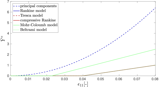
Figure 5: Various crack-driving forces $Y^{e}$ in uniaxial strain. The material parameters are: $E=10000\,$MPa, $\nu=0.25$, $\mathcal{G}_{c}=10\,$N/mm, $l_{c}=1\,$mm.

In Figure 5 all driving forces are plotted for the case of simple uniaxial tension. It can be seen that the driving force in the energy based criterion takes immediate effect whereas the stress-strain based crack-driving forces start from a threshold. Also, the ad-hoc crack-driving forces are smaller than the positive energy. This may require an adapted relaxation time $\tau$ in (6) or, correspondingly, a somewhat higher mobility parameter. The driving forces of maximum principal stress, maximum shear stress, extended principal stress and maximum principal strain coincide in the displayed loading case but not in general. Moreover, the slope of the driving force of the Mohr-Coloumb model depends on the choice of material parameter $m$.

In Table 1 all stated driving forces are summarized. Here we also define the short name of the models which will be referred to in our sample computations.

Table 1: Crack-driving forces for the phase-field evolution $\tau\dot{z}=\bar{Y}$ with $\bar{Y}=\bar{Y}^{e}+l_{c}\gamma$.

model	$\bar{Y}$	short name
elastic energy, $\delta_{z}\Psi^{e}$	$\bar{Y}^{e}=g^{\prime}\left(\frac{\lambda}{2}(\operatorname{tr}\bm{\epsilon})^{2}+\mu\bm{\epsilon}:\bm{\epsilon}\right)$	Griffith model
energy split (25), $\delta_{z}\Psi^{e}$	$\bar{Y}^{e}=g^{\prime}\left(\bm{\sigma}^{+}:\bm{\epsilon}^{+}\right)$	principal components
energy split (31), $\delta_{z}\Psi^{+}$	$\bar{Y}^{e}=g^{\prime}\left(\frac{\lambda}{2}\langle\operatorname{tr}\bm{\epsilon}\rangle_{+}^{2}+\mu(\bm{\epsilon}^{+})^{2}\right)$	$\lambda$-$\mu$ energy split
energy split (30), $\delta_{z}\Psi^{+}$	$\bar{Y}^{e}=g^{\prime}\left(\frac{K}{2}\langle\operatorname{tr}\bm{\epsilon}\rangle_{+}^{2}+\mu\operatorname{dev}(\bm{\epsilon}^{+})^{2}\right)$	$K$-$\mu$ energy split
maximum shear stress	$\bar{Y}^{e}=\left\langle\frac{\tau_{I}}{\tau_{c}}-1\right\rangle_{+}$	Tresca model
maximum principal stress	$\bar{Y}^{e}=\left\langle\frac{\sigma_{I}}{\sigma_{c}}-1\right\rangle_{+}$	Rankine model
extended principal stresses	$\bar{Y}^{e}=\mathds{1}_{\{\sigma_{m}>0\}}\left\langle\frac{\sigma_{I}}{\sigma_{c}}-1\right\rangle_{+}$	compressive Rankine
frictional shear stress	$\bar{Y}^{e}=\left\langle\frac{\sigma_{I}}{R_{m}^{t}}-\frac{\sigma_{III}}{R_{m}^{p}}-1\right\rangle_{+}$	Mohr-Coulomb model
maximum principal strain	$\bar{Y}^{e}=\left\langle\frac{\epsilon_{I}}{\epsilon_{c}}-1\right\rangle_{+}$	Beltrami model

4 Numerical examples

4.1 Plane mode-I tension and mode-II shear tests

\psfrag{U}[cc]{$\bar{u}$}\includegraphics[width=130.08731pt]{modeIsketch.eps}

\psfrag{U}[cc]{$\bar{u}$}\includegraphics[width=130.08731pt]{2017-10-26-LinearMiehe_PF_TS925.eps}

\psfrag{U}[cc]{$\bar{u}$}\includegraphics[width=130.08731pt]{2017-10-26-LinearMiehe_PF_TS984.eps}

Figure 6: Geometry and boundary conditions (left) of the mode-I tension test and the typical phase-field evolution after 925 and 984 uniform steps of loading (right)

At first we study a simple mode-I tension test and consider a $100\times 100\,$mm plate with a centered notch under plane stress condition; details of geometry and boundary conditions are shown in Fig. 6. If not mentioned otherwise, the plate is meshed uniformly with $100\times 100\times 4$ triangular finite elements with linear shape functions (P1 elements). Reference material data are an elastic modulus of ${E}=50\,400$N/mm², Poisson ratio $\nu=0.2$ and a critical Griffith energy of $\mathcal{G}_{c}=75\,{\text{N}}/{\text{m}}$; the critical length is $l_{c}=1\,$mm. From the one-dimensional crack solution (see Appendix A) the critical stress follows as

$$\sigma_{c}=\sqrt{\frac{E\mathcal{G}_{c}}{3l_{c}}}$$ (58)

which gives here $\sigma_{c}=35\,$N/mm². Vertical displacements are prescribed on the upper boundary with increments $\Delta\bar{u}=5\cdot 10^{-5}$mm.

4.1.1 Mode-I tension for different driving forces in linear elasticity

We start with a comparison of the energy driven crack growth, according to the Griffith and the $\lambda$-$\mu$ split model, and a stress driven crack growth according to the Rankine model. For all models the crack path is the same with the typical phase-field evolution shown in Fig. 6.

\psfrag{D}[cc]{\small{$\bar{u}$ [mm]}}\psfrag{F}[cc][cr]{\small{$F/F_{\text{max}}(\lambda$-$\mu\,\text{split})$ }}\includegraphics[width=195.12767pt]{20180529_TT_Linear_Energy.eps}

\psfrag{D}[cc]{\small{$\bar{u}$ [mm]}}\psfrag{F}[cc][cr]{\small{$F/F_{\text{max}}(\lambda$-$\mu\,\text{split})$ }}\includegraphics[width=195.12767pt]{20180518_Linear_EnergyVsStress_LVK.eps}

Figure 7: Load-displacement curve of the mode-I tension test for two energy based driving forces (left) and a comparison of the $\lambda$-$\mu$ energy split with the Rankine model (right).

From the load-displacement curve in Fig. 7 (left) it can be seen, that the crack starts propagating at a prescribed displacement of about $0.02\,$mm for both, the Griffith and $\lambda$-$\mu$ split model. Both curves almost coincide which can be explained by the overall tensile state in mode I. In Fig. 7 (right) the Rankine model is compared with the energy based approaches. They also show a very similar behavior and the crack starts propagating at a prescribed displacement of about $0.02$ mm. The remaining difference in maximum loading is caused by the definition of the critical stress via relation (58). Here the introduction of an additional weight for the Rankine model, as suggested in Miehe et al. (2015a), would allow to compute identical load-displacement curves for both, the energy and the stress driven crack. This only requires a careful calibration of the additional parameter, which, however, has no physical meaningful explanation.

4.1.2 Mode-I tension for different driving forces in finite elasticity

In a second step the tension test is computed in a finite deformation regime. We start with different energy based criteria, i.e. the multiplicative split of the eigenvalues (35) and the additive split of the invariants (40) are compared. Here we make use of a Neo-Hookean material model extended to the volumetric range with energy density (20-21) with $k=0$. The material data are the same as above; they result in $K=28\,000$N/mm² and $\mu=21\,000$N/mm².

\psfrag{D}[cc]{\small{$\bar{u}$ [mm]}}\psfrag{F}[cc][cr]{\small{$F/F_{\text{max}}(\text{energy (inv.)})$ }}\includegraphics[width=195.12767pt]{20180601_TT_Nonlinear_Energy.eps}

\psfrag{D}[cc]{\small{$\bar{u}$ [mm]}}\psfrag{F}[cc][cr]{\small{$F/F_{\text{max}}(\text{energy (inv.)})$ }}\includegraphics[width=195.12767pt]{20180524_TT_Nonlinear_EnergyVsStress.eps}

Figure 8: Load-displacement curve of the mode-I tension test for different anisotropic splits (left) and for the stress based criterion (right).

The phase-field simulation of the crack path is typical mode I. The related load-displacement curves are shown in Fig. 8. It can be seen that for the split of the invariants the crack starts propagating at about the same prescribed displacement as in the linear case. For the multiplicative split of the eigenvalues the load at crack initiation is about 20% lower. Although it runs numerically stable here, the eigenvalue split seems not to be the proper choice for the crack-driving force.

The load-displacement curves of the two different driving forces – energy split of the invariants and the Rankine model – are depicted in Fig. 8 (right). Here the behavior before crack initiation is linear in the stress-based approach whereas the energy based crack-driving force is sub-linear. For the Rankine model the crack starts propagating slightly earlier. The latter can be explained by the critical stress value $\sigma_{c}$ which is derived from linear elasticity and compared here with the Cauchy stress.

4.1.3 Effect of length scale parameter $l_{c}$

At next we study the influence of the regularization length $l_{c}$ on the fracture load. In the classical phase-field approach parameter $l_{c}$ has a two-fold effect. On the one hand, $l_{c}$ determines the diffusive crack width within the finite element discretization and is determined by the mesh size $h$. For crack evaluation $l_{c}>h$ is required and, depending on the approximation order, commonly $l_{c}=1.5\dots 3h$ is chosen. On the other hand, $l_{c}$ enters the fracture energy density by $\ \mathcal{G}_{c}/l_{c}$. Because in the classical approach the crack will grow when the elastic energy of the material exceeds the fracture energy, $l_{c}$ works here like a material parameter. In consequence, the classical phase-field approach is very sensitive against the choice of $l_{c}$.

The effect can be seen in the load-displacement curves of the linear mode-I model, plotted in Fig. 9, where we vary $l_{c}$ from 1 to 5 mm. In the Griffith model the maximal load magnifies with $l_{c}$ by a factor of almost 20. This is in opposite to the effect which $l_{c}$ has in stress or strain driven crack growth where $l_{c}$ enters only the crack width.

From the plots in Fig. 9 it is obvious, that the Rankine model shows less sensitivity to the choice of the length scale $l_{c}$. In order to quantify this observation, we listed the computed maximal loads for different $l_{c}$ in Tab. 2 and compared it to the diffusive ’crack volume’ of a crack with unit length in the one-dimensional solution, $V(l_{c})=\int_{0}^{1}\exp(|x|/l_{c})\,\mathrm{d}x$. The result is clear: the diffusive width $l_{c}$ effects the load required for crack growth basically in the same way as the diffusive crack volume changes. This is a major advantage of the Rankine crack-driving force, compared to the original phase-field model of Griffith energy driven crack growth.

Table 2: Diffusive crack volume and maximum load in the Rankine model for different $l_{c}$

$l_{c}$	[mm]	1	2	3	4	5
$V(l_{c})$	[mm${}^{3}]$	126	157	170	177	181
$V(l_{c})/V(1)-1\$	$[\%]$	0	25	35	40	44
$F_{\text{max}}(l_{c})\$	[kN]	93.5	117.5	133.3	145.1	154.2
$F_{\text{max}}(l_{c})/F_{\text{max}}(1)-1\$	$[\%]$	0	26	43	55	65

When in the Griffith model the ratio $\mathcal{G}_{c}/l_{c}$ is kept constant the computed maximal load is even higher. This was to expect and is not displayed extra but it also underlines that the Rankine model is much more stable to modifications of $l_{c}$. We remark that smaller time steps would result in spikier curves. The general result, however, is not affected by a varying mesh or time discretization and it holds for all stress or strain driven crack-driving forces of Table 1.

\psfrag{force}[cc][cr]{\small{$F_{\text{max}}/F_{\text{max}}(l_{c}=1)$ }}\psfrag{displacement}[cc][cc]{\small{$\bar{u}$ [mm]}}\includegraphics[height=177.78578pt]{GcSclc1und5.eps}

\psfrag{force}[cc][cr]{\small{$F_{\text{max}}/F_{\text{max}}(l_{c}=1)$ }}\psfrag{displacement}[cc][cc]{\small{$\bar{u}$ [mm]}}\includegraphics[height=177.78578pt]{Sclc1bis5.eps}

Figure 9: Variation of the critical length parameter $l_{c}$ for the Griffith model with constant $\mathcal{G}_{c}$ or $\mathcal{G}_{c}/l_{c}$ ratio (left) and for the Rankine model (right)

4.1.4 Effect of finite element discretization

For completeness we compare now the load-displacement curves for different finite element meshes and different crack-driving forces, Fig. 10. For a fixed $l_{c}$ –which is determined by the mesh size– we see only minor differences between a linear P1 and a quadratic P2 triangulation. A drawback of the quadratic approximation is that it tends to oscillate during unloading, affecting all phase-field models in a similar manner. A finer mesh results in a softer response of the model and, thus, in a smaller maximum loading. Additionally it can be seen from Fig. 10 that the Rankine model and the Beltrami model give very similar results.

\psfrag{force}[cc][cr]{\small{$F_{\text{max}}/F_{\text{max}}(l_{c}=1)$ }}\psfrag{displacement}[cc][cc]{\small{$\bar{u}$ [mm]}}\includegraphics[height=186.45341pt]{GcScEcP1P2.eps}

\psfrag{force}[cc][cr]{\small{$F_{\text{max}}/F_{\text{max}}(l_{c}=1)$ }}\psfrag{displacement}[cc][cc]{\small{$\bar{u}$ [mm]}}\includegraphics[height=186.45341pt]{ScEc_meshes.eps}

Figure 10: Effect of finite element approximation order: full energy driven, principal stress driven and principal strain driven crack growth for linear P1 and quadratic P2 triangulation (left) and principal stress driven crack growth for different mesh sizes (right)

4.1.5 Mode-II test

\psfrag{U}[cc]{$\bar{u}$}\psfrag{w}[cc][cc]{$\alpha$}\psfrag{A}[cc][bc]{Griffith model}\psfrag{B}[cc][cc]{principal axis split}\psfrag{C}[cc][cc]{$K$-$\mu$ energy split}\psfrag{D}[cc][cc]{$\lambda$-$\mu$ energy split}\psfrag{E}[cc][cc]{Tresca model}\psfrag{F}[cc][cc]{Rankine model}\psfrag{G}[cc][cc]{compressive Rankine }\psfrag{H}[cc][cc]{Mohr-Coloumb model}\psfrag{J}[cc][cc]{Beltrami model}\psfrag{K}[cc][cc]{inverse Mohr-Coloumb model}\includegraphics[width=429.28616pt]{20180529_Sheartest2D.eps}

Figure 11: Mode-II-shear test with different crack-driving forces

Because the tension test is too simple to compare the different crack-driving forces, we change the boundary conditions of our computational model now to a shear test. This situation has been used for numerous investigations on the direction of kinking cracks. Different theoretical approaches have been developed, e.g. the principle of local symmetry, which states that the crack propagates in such a way that the mode-II stress intensity factor vanishes in the vicinity of the crack tip, Amestoy and Leblond (1992); Goldstein and Salganik (1974); Hodgdon and Sethna (1993); Leblond (1989); Katzav et al. (2007). Alternatively the direction of crack growth can be determined so that it minimizes the potential energy or maximizes the energy release rate among all kinking angles, Erdogan and Sih (1963); Bilby and Cardew (1975); Chambolle et al. (2009). Experiments under shear have been performed, for example, by Erdogan and Sih Erdogan and Sih (1963). They observed a crack declined by an angle of $\alpha=110^{\circ}$ in sheared PMMA and mentioned also, that the kinking direction strongly depends on the ’brittleness’ of the material.

In this sense we study here the effect of all crack-driving forces in shearing. We start with a linear elastic plane stress computation and observe different kinking angles, Fig. 11. The full elastic energy of the Griffith model would drive a straight crack growth which is shear dominated and does not kink. The different energy splits give similar and realistic results, but in detail the kinking angles differ between $129^{\circ}$ and $134^{\circ}$. The Tresca model, which accounts for shear only, gives a straight $180^{\circ}$ crack growth. This may be observed in ductile metals. The Rankine model of maximal principal stresses results in a kinking angle of $122^{\circ}$, the compressive Rankine model reduces this angle to $117^{\circ}$ and gives the steepest kink. Quite interesting results gives the Mohr-Coloumb model which accounts for tension and shear. If we assume a tension sensitive material ($m=10$) the crack kinks as in the previous models with $124^{\circ}$ whereas a compression sensitive material ($m=0.1$) like, e.g. foam, shows a completely opposite behavior with a shear induced crack towards the upper side of the model. At last, the Beltrami model of maximal principal strains behaves similar to the principal stress model with a kinking angle of $131^{\circ}$.

In Fig. 12 the crack evolution in the mode-II shear test for the different finite elasticity models is displayed. Here again, the different energy splits give different results but the best result —in comparison to the experiments in Erdogan and Sih (1963)— gives the Rankine model of maximum principal stresses. For all models the stress driven crack growth is similar to the linear elastic regime whereby the kinking angle is always somewhat smaller. This may in part be due to the fully three-dimensional computation.

In total we may summarize, that the generalized driving force model offers the opportunity to describe crack characteristics, like as the kinking angle under shear, as it is observed in practise. The right choice of the crack-driving force depends on the properties of the specific material.

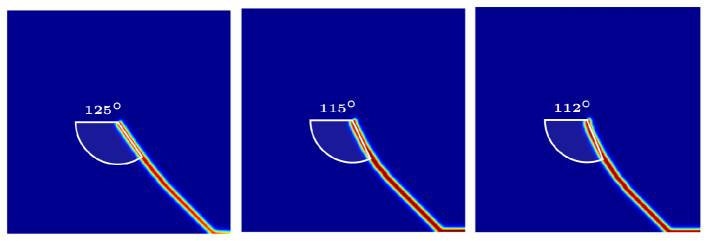
Figure 12: Phase-field snapshots of the two dimensional sheartest for the different models - anisotropic split of the eigenvalues with $\alpha=125\textdegree$ (left), anisotropic split of the invariants with $\alpha=115\textdegree$ (middle) and the Rankine-model with $\alpha=112\textdegree$ (right).

4.2 Brazilian test simulations

The Brazilian or compressive-split test of civil engineering is a popular experiment to determine the tensile strength of brittle, tension-sensitive material. Two opposing forces are applied to the cross section of a cylindrical specimen until a tension, perpendicular to the loading direction, causes the specimen to crack. The Brazilian test with quasi-static loading is standardized, e.g. in ASTM C496 and DIN EN 12390-6, and determines the tensile resistance of the specimen as

$$R_{m}^{\text{t}}=\frac{2F_{\text{max}}}{\pi LD}$$ (59)

where $F_{\text{max}}$, $L$ and $D$ are maximum applied load, length and diameter of the specimen, respectively.

\psfrag{D}[cl][cc]{\small{$D=50\,$mm}}\psfrag{b}[cc][cc]{\small{$b$}}\psfrag{u}[cc][cc]{\small{$\bar{u}$}}\includegraphics[width=121.41306pt]{2_new.eps}

\psfrag{D}[cl][cc]{\small{$D=50\,$mm}}\psfrag{b}[cc][cc]{\small{$b$}}\psfrag{u}[cc][cc]{\small{$\bar{u}$}}\includegraphics[width=160.43727pt]{brazspecgeometry}

\psfrag{D}[cl][cc]{\small{$D=50\,$mm}}\psfrag{b}[cc][cc]{\small{$b$}}\psfrag{u}[cc][cc]{\small{$\bar{u}$}}\includegraphics[width=117.07924pt]{picUHPC}

Figure 13: UHPC Brazilian disc specimen: dynamic cracking (left), specimen geometry (middle) and cracked specimen geometry (right)

\psfrag{A}[cc][cc]{\small{Griffith model}}\psfrag{B}[cc][cc]{\small{$\lambda$-$\mu$-split}}\psfrag{C}[cc][cc]{\small{Rankine model}}\includegraphics[width=195.12767pt]{braz33169Griffith.eps}

\psfrag{A}[cc][cc]{\small{Griffith model}}\psfrag{B}[cc][cc]{\small{$\lambda$-$\mu$-split}}\psfrag{C}[cc][cc]{\small{Rankine model}}\includegraphics[width=195.12767pt]{braz33169Rankine.eps}

Figure 14: Crack pattern of the Brazilian disc specimen for different crack-driving forces: Griffith model (left) and Rankine model (right)

In Khosravani et al. (2018) we performed dynamic Brazilian test with specimens made of Ultra-High Performance Concrete (UHPC), whereby the evaluation of the tensile resistance is the same as in statics, Eq. (59). Setup, geometry and a cracked specimen are displayed in Fig. 13 and serve us here as a reference to study phase-field fracture simulations. Our finite element model consists of 33 169 P1 elements. A successive compressive displacement in axial direction is prescribed from both sides. At the two center points also the lateral displacement is constraint. The specimen has the typical material data of UHPC, $E=50\,000\,$MPa, $\nu=0.2$, $R_{m}^{\text{t}}=\sigma_{c}=17\,$MPa and $G_{c}=70\,$N/m.

Please note that the analytical derivation of equation (59) presumes a circular linear-elastic disc with point loads $F$, Fro . The principal tensile stress, $\sigma_{I}$, which has its maximum in the center of the disc, is then identified with the resistance (59). The value of the compressive stress in the specimen is much higher. From the practical point of view, the major criterium for a valid Brazilian test is that the crack starts in the center of the disc. This happens only for materials with a strong tension-compression asymmetry. Other brittle materials like glass or some plastics fail the test because their cracking starts at the support.

Figure 14 shows the computed specimen for different crack-driving forces. All the energy criteria fail to give realistic crack patterns. In our computation this means at the loading zone a rapid loss of stiffness down to the $\varepsilon$-value of the degradation function (28). Further results are then meaningless. Realistic crack pattern in the sense of a valid Brazilian test gives only the Rankine model and, slightly different, the compressive Rankine model. In both models the crack starts in the center of the disc and grows rapidly towards the boundary.

The maximum applied force per thickness in the Rankine model is $F_{\text{max}}=3300\,$N/mm which is roughly in the range of the value $F_{\text{max}}=2750\,$N/mm expected from Eq. (59). The calculated force depends on the crack-driving force but also on the boundary conditions and will be elaborated in more detail in a subsequent work. Here we summarize that, regarding the theoretical basis of the experiment, only the phase-field crack-driving force determined by the maximum tensile stress models the Brazilian test adequately.

4.3 A conchoidal fracture example

Finally a three dimensional example is studied to demonstrate the effect of different crack-driving forces. We focus on a specific type of brittle fracture known as conchoidal fracture. Conchoidal fracture can be observed in fine-grained or amorphous materials, such as rock and glass, and is characterized by cleavage without any natural planes of separation. It results in a curved surface with ripples, the so called Wallner lines Wallner (1939), that resembles the surface of a sea shell. In Bilgen et al. (2017) phase-field fracture computations are performed on two conchoidal fracture examples and a series of investigations were carried out, mainly focussing on a fast numerical scheme for the classical approach. Here we want to extend these results by applying different crack-driving forces in the phase-field model.

The geometry of the problem is illustrated in Fig. 15. A three-dimensional $4a\times 4a\times 2a$ bloc of brittle material is loaded by a vertical displacement on part of its upper boundary, $2a=1\,$m. On the lower boundary, Dirichlet conditions $\bm{u}=0$ and $z=0$ for the displacements and the phase-field are prescribed.

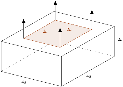
Figure 15: Geometry and loading of a bloc of brittle material.

4.3.1 Linear-elastic analysis

The stone-like material has an elastic modulus of $E=250000\ \nicefrac{{\text{N}}}{{\text{mm}^{2}}}$, a Poisson’s ratio of $\nu=0.25$ and a Griffith energy of $\mathcal{G}_{c}=1\ \text{N}/\text{mm}$. We use a finite element mesh which consists of $27000$ 8-node brick elements, such that the geometry can be resolved with a length scale parameter of $l_{c}=0.2\,$m. The displacement-driven deformation with increments of $\Delta\bar{u}=0.0001\,$mm is prescribed up to complete failure.

Snapshots of the phase-field evolution at different time steps can be seen in Fig. 16. For the displayed maximum-stress driven crack (Rankine model) as well as for all energy-split driven models the crack starts propagating inside of the bloc below the pulled surface. Please note that this crack nucleation happens in a completely homogenous material without any notch or flaw. Once nucleated the crack is characterized by brutal growth until complete failure.

In the iso-surface the typical rippled surface of conchoidal fracture can be observed. The crack nucleates at a displacement of approximately $0.003\,$m , see Fig. 17. As already noticed in the previous examples the maximum load of crack initiation differs slightly for the different driving forces.

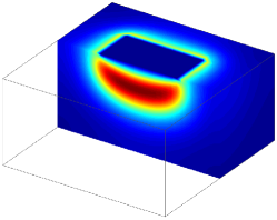
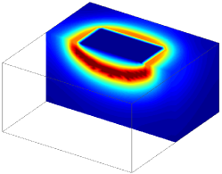
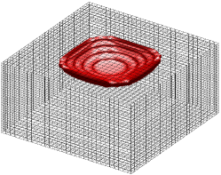
Figure 16: Phase-field snapshots applying the Rankine model formulation at time step 20 (left), time step 30 (middle) and iso-surface at time step 30 (right).

\psfrag{D}[cc]{\small{$\bar{u}$ [mm]}}\psfrag{F}[cc][cr]{\small{$F$ [N] }}\includegraphics[width=303.53267pt]{20180625_BM3D_FailureCrit.eps}

Figure 17: Load-displacement curves of the conchoidal fracture example for different crack-driving forces. The names in the legend refer to the models of Table 1.

In a next step we want to examine the Mohr-Coulomb crack-driving force in more detail. Because this model depends not only on the tensile strength $R_{m}^{t}$ but also on the compressive strength $R_{m}^{p}$ we investigate different relations between these two parameters. In Fig. 18 different load-displacement curves are displayed. The curves with $R_{m}^{t}>R_{m}^{p}$ have a very similar shape; the graph with $R_{m}^{t}<R_{m}^{p}$ differs. This is confirmed by the phase-field snapshots of Fig. 19 which shows that only for $R_{m}^{t}>R_{m}^{p}$ the crack nucleates inside the bloc and leads to the specific shell-like breakage. For $R_{m}^{t}<R_{m}^{p}$ the crack starts growing at the upper surface. These different mechanisms are caused by the reverse influence of the compressive and tensile states in the driving force.

\psfrag{D}[cc]{\small{$\bar{u}$ [mm]}}\psfrag{F}[cc][cr]{\small{$F$ [N]}}\includegraphics[width=303.53267pt]{20180625_BM3D_MC.eps}

Figure 18: Load-displacement curves of the conchoidal fracture example for the Mohr-Coulomb crack-driving force with different ratios of $R_{m}^{p}/R_{m}^{t}=m$.

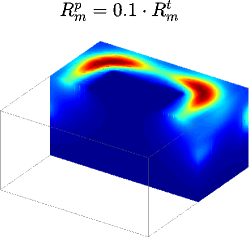
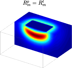
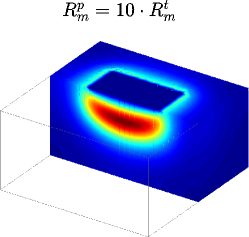
Figure 19: Phase-field snapshots for the Mohr-Coulomb crack-driving force for various relations of $R_{m}^{p}$ and $R_{m}^{t}$.

4.3.2 Finite deformation analysis

Finally, the proposed theory is applied in finite elasticity by decreasing the elastic modulus $E$ of this conchoidal fracture example down to a rubbery behavior of the block. The remaining properties of the material are kept constant as $\nu=0.25$ and the Griffith energy as $\mathcal{G}_{c}=1$ N/mm and follow now a Neo-Hookean material model with energy density (20-21) and $k=0$. The results of the phase-field fracture computations are displayed in Fig. 20 and 21. All computations result in the typical conchoidal crack surface which is initiated inside the bloc. The load-displacement curves show that with lower elastic modulus $E$ the prescribed displacement at crack initiation is higher. The force, however, is almost constant and determined by the material parameter.

We remark, that everybody may observe such conch-like fracture surfaces of soft material in ’ruptured’ Swiss cheese for example.

\psfrag{D}[cc]{\small{$\bar{u}$ [mm]}}\psfrag{F}[cc][cr]{\small{$F$ [N]}}\includegraphics[width=303.53267pt]{20180517_BM3D_VaryE.eps}

Figure 20: Load-displacement curves of the conchoidal fracture example with different elastic modulus $E$.

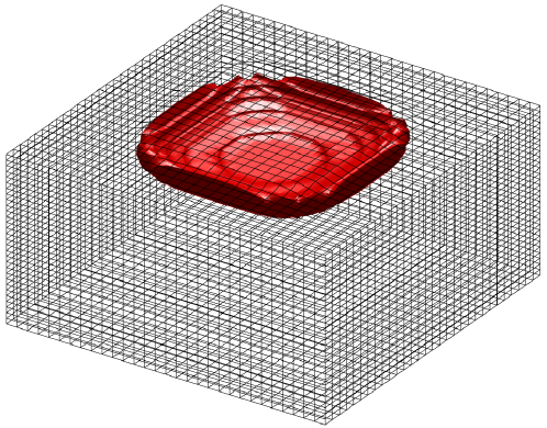
Figure 21: Conchoidal fracture surface as a result of rupture in the block with $E=10000\,\mathrm{N/mm^{2}}$.

5 Concluding remarks

The popular phase-field model of fracture in quasi-brittle materials is based on a variational approach of energy optimization. It has a sound mathematical basis and is known to converge for regularization length $l_{c}\to 0$ to Griffith’ sharp interface model of brittle fracture. For general numerical computations, however, the crack-driving force cannot follow from the same potential then the deformation field. The physical restriction that crack growth presumes a state of tension, requires a split of the body’s energy into tensional, crack-driving components and insensitive compressive remainders. In consequence, the energy minimization needs to be performed in a hybrid variational form with different potentials for phase-field and deformation.

This hybrid form is neither unique nor obvious from the physical point of view. Therefore we suggest here, to drive the evolution of the phase-field without energy minimization, using physically motivated and ad-hoc formulated driving forces instead. We introduce different versions of crack-driving forces, compare their pros and cons and perform several numerical computations to illustrate their applicability. In particular we point out that practical examples, like the Brazilian test of concrete and the conchoidal fracture of glassy material, require a crack-driving force specifically derived from fracture mechanics.

Appendix

To find a relation between the Griffith energy $\mathcal{G}_{c}$ and the fracture strain $\epsilon_{c}$ in phase-field fracture we consider a crack in one dimension. With energy $\Psi^{e}_{0}=\frac{1}{2}E\epsilon^{2}$, degradation function $g(z)=(1-z)^{2}$ and crack-surface density function (4) the variation of energy gives

$$2(1-z)\Psi^{e}_{0}-\frac{\mathcal{G}_{c}}{l_{c}}\left(z-l_{c}^{2}\triangle z\right)=0\,.$$

Now we neglect the regularizing terms to obtain

$$\left(2\frac{l_{c}}{\mathcal{G}_{c}}\Psi^{e}_{0}+1\right)(1-z)=1$$

Resolving for $1-z$ and with the degradated form of (13) it follows a non-monotonous function for the degrading stresses

$$\sigma=g(z)E\epsilon=\left(\frac{l_{c}}{\mathcal{G}_{c}}E\epsilon^{2}+1\right)^{-2}E\epsilon\,.$$

Its maximum value defines the critical fracture strain $\epsilon_{c}$.

$$\epsilon_{c}=\sqrt{\frac{\mathcal{G}_{c}}{3l_{c}E}}$$

References

- (1)
- Ambati et al. (2015) M. Ambati, T. Gerasimov, and L. De Lorenzis. Phase-field modeling of ductile fracture. Computational Mechanics, 55(5):1017–1040, 2015.
- Ambati et al. (2016) M. Ambati, R. Kruse, and L. De Lorenzis. A phase-field model for ductile fracture at finite strains and its experimental verification. Computational Mechanics, 57(1):149–167, 2016.
- Ambrosio and Tortorelli (1990) L. Ambrosio and V. M. Tortorelli. Approximation of functionals depending on jumps by elliptic functionals via -convergence. Communications on Pure and Applied Mathematics, 43(8):999–1036, 1990. ISSN 1097-0312. doi: 10.1002/cpa.3160430805. URL http://dx.doi.org/10.1002/cpa.3160430805.
- Amestoy and Leblond (1992) M. Amestoy and J. Leblond. Crack paths in plane situations - ii. detailed form of the expansion of the stress intensity factors. International Journal of Solids and Structures, 29:465–501, 1992.
- Amor et al. (2009) H. Amor, J.-J. Marigo, and C. Maurini. Regularized formulation of the variational brittle fracture with unilateral contact: Numerical experiments. Journal of the Mechanics and Physics of Solids, 57(8):1209–1229, 2009.
- Bilby and Cardew (1975) B. Bilby and G. Cardew. The crack with a kinked tip. International Journal of Fracture, 11(4):708–712, 1975.
- Bilgen et al. (2017) C. Bilgen, A. Kopaničáková, R. Krause, and K. Weinberg. A phase-field approach to conchoidal fracture. Meccanica, pages 1–17, 2017.
- Bleyer and Alessi (2018) J. Bleyer and R. Alessi. Phase-field modeling of anisotropic brittle fracture including several damage mechanisms. Computer Methods in Applied Mechanics and Engineering, 336:213–236, 2018.
- Borden et al. (2012) M. Borden, C. Verhoosel, M. Scott, T. Hughes, and C. Landis. A phase-field description of dynamic brittle fracture. Comput. Methods Appl. Mech. Engrg., 217–220:77–95, 2012.
- Borden et al. (2014) M. J. Borden, T. J. Hughes, C. M. Landis, and C. V. Verhoosel. A higher-order phase-field model for brittle fracture: Formulation and analysis within the isogeometric analysis framework. Computer Methods in Applied Mechanics and Engineering, 273(0):100 – 118, 2014. ISSN 0045-7825. doi: http://dx.doi.org/10.1016/j.cma.2014.01.016. URL http://www.sciencedirect.com/science/article/pii/S0045782514000292.
- Bourdin et al. (2008) B. Bourdin, G. Francfort, and J.-J. Marigo. The Variational Approach to Fracture. Springer-Verlag, 2008.
- Chambolle et al. (2009) A. Chambolle, G. A. Francfort, and J.-J. Marigo. When and how do cracks propagate? Journal of the Mechanics and Physics of Solids, 57(9):1614–1622, 2009.
- Dally and Weinberg (2017) T. Dally and K. Weinberg. The phase-field approach as a tool for experimental validations in fracture mechanics. Continuum Mechanics and Thermodynamics, 29(4):947–956, 2017.
- Doll and Schweizerhof (2000) S. Doll and K. Schweizerhof. On the development of volumetric strain energy functions. Journal of Applied Mechanics, 67:17–20, 2000.
- Ehlers and Luo (2017) W. Ehlers and C. Luo. A phase-field approach embedded in the theory of porous media for the description of dynamic hydraulic fracturing. Computer Methods in Applied Mechanics and Engineering, 315:348–368, 2017.
- Erdogan and Sih (1963) F. Erdogan and G. Sih. On the crack extension in plates under plane loading and transverse shear. Journal of basic engineering, 85(4):519–525, 1963.
- Francfort and Marigo (1998) G. Francfort and J.-J. Marigo. Revisiting brittle fracture as an energy minimization problem. Journal of the Mechanics and Physics of Solids, 46:1319–1342, 1998. doi: 10.1016/S0022-5096(98)00034-9. URL http://dx.doi.org/10.1016/S0022-5096(98)00034-9.
- Freddi and Royer-Carfagni (2010) F. Freddi and G. Royer-Carfagni. Regularized variational theories of fracture: a unified approach. Journal of the Mechanics and Physics of Solids, 58(8):1154–1174, 2010.
- Goldstein and Salganik (1974) R. Goldstein and R. Salganik. Brittle fracture of solids with arbitrary cracks. International Journal of Fracture, 10:507–523, 1974.
- Gross and Selig (2011) D. Gross and T. Selig. Bruchmechanik - Mit einer Einf hrung in die Mikromechanik. Springer, 5. auflage edition, 2011.
- Hartmann and Neff (2003) S. Hartmann and P. Neff. Polyconvexity of generalized polynomial-type hyperelastic strain energy functions for near-incompressibility. Int. J. Solids and Structures, 40:2767–2791, 2003.
- Heider and Markert (2017) Y. Heider and B. Markert. A phase-field modeling approach of hydraulic fracture in saturated porous media. Mechanics Research Communications, 80:38–46, 2017.
- Henry and Levine (2004) H. Henry and H. Levine. Dynamic instabilities of fracture under biaxial strain using a phase field model. Physics Review Letters, 93:105505, 2004.
- Hesch et al. (2016) C. Hesch, S. Schuß, M. Dittmann, M. Franke, and K. Weinberg. Isogeometric analysis and hierarchical refinement for higher-order phase-field models. Computer Methods in Applied Mechanics and Engineering, 303:185–207, 2016.
- Hesch et al. (2017) C. Hesch, A. J. Gil, R. Ortigosa, M. Dittmann, C. Bilgen, P. Betsch, M. Franke, A. Janz, and K. Weinberg. A framework for polyconvex large strain phase-field methods to fracture. Computer Methods in Applied Mechanics and Engineering, 317:649–683, 2017.
- Hodgdon and Sethna (1993) J. Hodgdon and J. Sethna. Derivation of a general threedimensional crack-propagation law - a generalization of the principle of local symmetry. Physical Review, 47:4831–4840, 1993.
- Karma et al. (2001) A. Karma, D. Kessler, and H. Levine. Phase-field model of mode iii dynamic fracture. Physical Review Letter, 81:045501, 2001.
- Katzav et al. (2007) E. Katzav, M. Adda-Bedia, and B. Derrida. Fracture surfaces of heterogeneous materials: a 2d solvable model. EPL (Europhysics Letters), 78(4):46006, 2007.
- Khosravani et al. (2018) M. R. Khosravani, M. Silani, and K. Weinberg. Fracture studies of ultra-high performance concrete using dynamic brazilian tests. Theoretical and Applied Fracture Mechanics, 93:302–310, 2018.
- Kuhn et al. (2016) C. Kuhn, T. Noll, and R. Müller. On phase field modeling of ductile fracture. GAMM-Mitteilungen, 39(1):35–54, 2016.
- Leblond (1989) J. Leblond. Cracks paths in plane situations - i. general form of the expansion of the stress intensity factors. International Journal of Solids and Structures, 362:295–296, 1989.
- Li et al. (2016) T. Li, J.-J. Marigo, D. Guilbaud, and S. Potapov. Gradient damage modeling of brittle fracture in an explicit dynamics context. International Journal for Numerical Methods in Engineering, 108(11):1381–1405, 2016.
- Miehe and Schänzel (2014) C. Miehe and L.-M. Schänzel. Phase field modeling of fracture in rubbery polymers. part i: Finite elasticity coupled with brittle failure. Journal of the Mechanics and Physics of Solids, 65:93–113, 2014.
- Miehe et al. (2010) C. Miehe, M. Hofacker, and F. Welschinger. A phase field model for rate-independent crack propagation: Robust algorithmic implementation based on operator splits. Comput. Methods Appl. Mech. Engrg., 199:2765–2778, 2010.
- Miehe et al. (2015a) C. Miehe, M. Hofacker, L.-M. Schänzel, and F. Aldakheel. Phase field modeling of fracture in multi-physics problems. part ii. coupled brittle-to-ductile failure criteria and crack propagation in thermo-elastic-plastic solids. Computer Methods in Applied Mechanics and Engineering, 294:486–522, 2015a.
- Miehe et al. (2015b) C. Miehe, L.-M. Sch nzel, and H. Ulmer. Phase-field modeling of fracture in multi-physics problems. part i. balance of crack surface and failure criteria for brittle crack propagation in thermo-elasitc solids. Comput. Methods Appl. Mech. Engrg., 294:449–485, 2015b.
- Negri (2013) M. Negri. From phase field to sharp cracks: Convergence of quasi-static evolutions in a special setting. Applied Mathematics Letters, 26(2):219–224, 2013.
- Sargado et al. (2018) J. M. Sargado, E. Keilegavlen, I. Berre, and J. M. Nordbotten. High-accuracy phase-field models for brittle fracture based on a new family of degradation functions. Journal of the Mechanics and Physics of Solids, 111:458–489, 2018.
- Teichtmeister et al. (2017) S. Teichtmeister, D. Kienle, F. Aldakheel, and M.-A. Keip. Phase field modeling of fracture in anisotropic brittle solids. International Journal of Non-Linear Mechanics, 97:1–21, 2017.
- Thomas et al. (2018) M. Thomas, C. Bilgen, and K. Weinberg. Phase‐field fracture at finite strains based on modified invariants: A note on its analysis and simulations. GAMM-Mitteilungen, 40 (3):207–237, 2018. doi: 10.1002/gamm.201730004.
- Verhoosel and de Borst (2013) C. Verhoosel and R. de Borst. A phase-field model for cohesive fracture. Int. J. Numer. Methods Eng., 2013.
- Wallner (1939) H. Wallner. Linienstrukturen an bruchflächen. Zeitschrift für Physik, 114(5-6):368–378, 1939.
- Weinberg and Hesch (2015) K. Weinberg and C. Hesch. A high-order finite-deformation phase-field approach to fracture. Continuum Mech. Thermodyn., 2015. doi: 10.1007/s00161-015-0440-7.
- Weinberg et al. (2016) K. Weinberg, T. Dally, S. Schuß, M. Werner, and C. Bilgen. Modeling and numerical simulation of crack growth and damage with a phase field approach. GAMM-Mitteilungen, 39(1):55–77, 2016.