Approach to thermal equilibrium in harmonic crystals with polyatomic lattice

Vitaly A. Kuzkin111Peter the Great Saint Petersburg Polytechnical University; Institute for Problems in Mechanical Engineering RAS; e-mail: kuzkinva@gmail.com
Abstract

We study transient thermal processes in infinite harmonic crystals with complex (polyatomic) lattice. Initially particles have zero displacements and random velocities such that distribution of temperature is spatially uniform. Initial kinetic and potential energies are different and therefore the system is far from thermal equilibrium. Time evolution of kinetic temperatures, corresponding to different degrees of freedom of the unit cell, is investigated. It is shown that the temperatures oscillate in time and tend to generally different equilibrium values. The oscillations are caused by two physical processes: equilibration of kinetic and potential energies and redistribution of temperature among degrees of freedom of the unit cell. An exact formula describing these oscillations is obtained. At large times, a crystal approaches thermal equilibrium, i.e. a state in which the temperatures are constant in time. A relation between equilibrium values of the temperatures and initial conditions is derived. This relation is refereed to as the non-equipartition theorem. For illustration, transient thermal processes in a diatomic chain and graphene lattice are considered. Analytical results are supported by numerical solution of lattice dynamics equations.

Keywords: thermal equilibrium; stationary state; approach to equilibrium; polyatomic lattice; complex lattice; kinetic temperature; harmonic crystal; transient processes; equipartition theorem; non-equipartition theorem; temperature matrix.

1 Introduction

In classical systems at thermal equilibrium, the kinetic energy of thermal motion of atoms is usually equally shared among degrees of freedom. This fact follows from the equipartition theorem [26, 62]. The theorem allows to characterize thermal state of the system by a single scalar parameter, notably the kinetic temperature, proportional to kinetic energy of thermal motion.

Far from thermal equilibrium, kinetic energies, corresponding to different degrees of freedom, can be different [8, 17, 24, 25, 27, 45]. Therefore in many works several temperatures are introduced [8, 17, 30, 31, 45]. For example, it is well known that temperatures of a lattice and electrons in solids under laser excitation are different (see e.g. a review paper [45]). Two temperatures are also observed in molecular dynamics simulations of shock waves. In papers [25, 24, 27, 60] it is shown that kinetic temperatures, corresponding to thermal motion of atoms along and across the shock wave front are different. Different nonequilibrium temperatures of sublattices of methylammonium lead halide are reported in papers [10, 17]. In papers [32, 33], stationary heat transfer in a harmonic diatomic chain connecting two thermal reservoirs is considered. It is shown that temperatures of sublattices at the nonequilibrium steady state are different.

In the absence of external excitations, the nonequilibrium system tends to thermal equilibrium. Approach to thermal equilibrium is accompanied by several physical processes. Distribution of velocities tends to Gaussian [23, 14, 35, 43, 57]. The total energy is redistributed among kinetic and potential forms [1, 35, 37, 41]. Kinetic energy is redistributed between degrees of freedom [41]. The energy is redistributed between normal modes [52]. These processes, except for the last one, are present in both harmonic and anharmonic systems [1, 14, 35, 37, 41, 43, 57]. In harmonic crystals, energies of normal modes do not equilibrate. However distribution of kinetic temperature in infinite harmonic crystals tends to become spatially and temporary uniform [23, 57, 42]. Therefore the notion of thermal equilibrium is widely applied to infinite harmonic crystals [7, 13, 14, 15, 22, 29, 43, 57, 59].

Approach to thermal equilibrium in harmonic crystals is studied in many works [7, 13, 14, 15, 22, 23, 29, 35, 37, 40, 41, 42, 43, 44, 50, 57]. Various aspect of this process are studied, including existence of the equilibrium state [43], ergodicity [59, 22], convergence of the velocity distribution function [7, 35, 14, 15], evolution of entropy [28, 29, 56] etc. In the present paper, we focus on the behavior of the main observable, notably kinetic temperature (temperatures).

Two different approaches for analytical treatment of harmonic crystals are presented in literature. One approach employs an exact solution of equations of motion [18, 23, 35, 29, 44]. Given known the exact solution, kinetic temperature is calculated as mathematical expectation of corresponding kinetic energy. For example, in pioneering work of Klein and Prigogine [35], transition to thermal equilibrium in an infinite harmonic one-dimensional chain with random initial conditions is investigated. Using exact solution derived by Schrödinger [55], it is shown that kinetic and potential energies of the chain oscillate in time and tend to equal equilibrium values [35]. Another approach uses covariances222Covariance of two centered random values is equal to mathematical expectation of their product. of particle velocities and displacements as main variables. For harmonic crystals, closed system of equations for covariances can be derived in steady [32, 47, 53] and unsteady cases [37, 40, 41, 42, 19, 48]. Solution of these equations describes, in particular, time evolution of kinetic temperature. In papers [37, 40, 41, 42], this idea is employed for description of approach to thermal equilibrium in harmonic crystals with simple (monoatomic) lattice333A lattice is referred to as simple lattice, if it coincides with itself under shift by a vector connecting any two particles.. In particular, monoatomic one-dimensional chains [2, 37] and two-dimensional lattices [42, 40, 41] have been covered.

In the present paper, we study approach towards thermal equilibrium in an infinite harmonic crystal with polyatomic lattice444Polyatomic lattice consists of several simple monoatomic sublattices. For example, graphene lattice consists of two triangular sublattices.. Our main goals are to describe time evolution of kinetic temperatures, corresponding to different degrees of freedom of the unit cell, and to calculate equilibrium values of these temperatures.

The paper is organized as follows. In section 2, equations of motion for the unit cell are represented in a matrix form. It allows to cover monoatomic and polyatomic lattices with interaction of an arbitrary number of neighbors and harmonic on-site potential. In section 3, approach to thermal equilibrium is considered. An equation describing the behavior of kinetic temperatures, corresponding to different degrees of freedom of the unit cell, is derived. An exact solution of this equation is obtained. In section 4, an expression relating equilibrium values of the temperatures with initial conditions is derived. In sections 5, 6, approach to thermal equilibrium in a diatomic chain and graphene lattice are studied. Obtained results are exact in the case of spatially uniform distribution of temperature in harmonic crystals. Implications of the nonuniform temperature distribution and anharmonic effects are discussed in the last section.

2 Equations of motion and initial conditions

We consider infinite crystals with complex (polyatomic) lattice in d𝑑d-dimensional space, d=1,2,3𝑑123d=1,2,3. In this section, equations of motion of the unit cell are written in a matrix form, convenient for analytical derivations.

Unit cells of the lattice are identified by position vectors, 𝐱𝐱\boldsymbol{\mathrm{x}}{}, of their centers555For analytical derivations, position vectors are more convenient than indices, because number of indices depends on space dimensionality.. Each elementary cell has N𝑁N degrees of freedom ui(𝐱),i=1,..,Nu_{i}(\boldsymbol{\mathrm{x}}{}),i=1,..,N, corresponding to components of particle displacements. The components of displacements form a column:

𝐮(𝐱)=(u1,u2,..,uN),\boldsymbol{\mathrm{u}}{}(\boldsymbol{\mathrm{x}}{})=(u_{1},u_{2},..,u_{N})^{\top}, (1)

where top\top stands for the transpose sign.

Particles from the cell 𝐱𝐱\boldsymbol{\mathrm{x}}{} interact with each other and with particles from neighboring unit cells, numbered by index α𝛼\alpha. Vector connecting the cell 𝐱𝐱\boldsymbol{\mathrm{x}}{} with neighboring cell number α𝛼\alpha is denoted 𝐚α\boldsymbol{\mathrm{a}}{}_{\alpha}. Centers of unit cells always form a simple lattice, therefore numbering can be carried out so that vectors 𝐚α\boldsymbol{\mathrm{a}}{}_{\alpha} satisfy the identity:

𝐚=α𝐚.α\boldsymbol{\mathrm{a}}{}_{\alpha}=-\boldsymbol{\mathrm{a}}{}_{-\alpha}. (2)

Here 𝐚=00\boldsymbol{\mathrm{a}}{}_{0}=0. Vectors 𝐚α\boldsymbol{\mathrm{a}}{}_{\alpha} for a sample lattice are shown in figure 1.
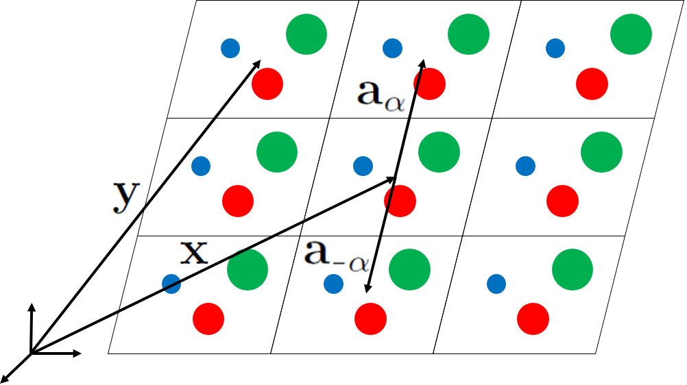
Refer to caption
Figure 1: Example of a complex two-dimensional lattice with three sublattices. Particles forming sublattices have different color and size.

Consider equations of motion of the unit cell. In harmonic crystals, the total force acting on each particle is represented as a linear combination of displacements of all other particles. Using this fact, we write equations of motion in the form666Similar form of equations of motion is used in paper [50].:

𝐌𝐯˙(𝐱)=α𝐂𝐮α(𝐱+𝐚)α,𝐂=α𝐂,α\begin{array}[]{l}\displaystyle\boldsymbol{\mathrm{M}}{}{}\dot{\boldsymbol{\mathrm{v}}{}}(\boldsymbol{\mathrm{x}}{})=\sum_{\alpha}\boldsymbol{\mathrm{C}}{}_{\alpha}\boldsymbol{\mathrm{u}}{}(\boldsymbol{\mathrm{x}}{}+\boldsymbol{\mathrm{a}}{}_{\alpha}),\qquad\boldsymbol{\mathrm{C}}{}_{\alpha}=\boldsymbol{\mathrm{C}}{}_{-\alpha}^{\top},\end{array} (3)

where 𝐯=𝐮˙𝐯˙𝐮\boldsymbol{\mathrm{v}}{}=\dot{\boldsymbol{\mathrm{u}}{}}; 𝐮(𝐱+𝐚)α\boldsymbol{\mathrm{u}}{}(\boldsymbol{\mathrm{x}}{}+\boldsymbol{\mathrm{a}}{}_{\alpha}) is a column of displacements of particles from unit cell α𝛼\alpha; 𝐌𝐌\boldsymbol{\mathrm{M}}{}{} is diagonal N×N𝑁𝑁N\times N matrix composed of particles’ masses; for α0𝛼0\alpha\neq 0 coefficients of N×N𝑁𝑁N\times N matrix 𝐂α\boldsymbol{\mathrm{C}}{}_{\alpha} determine stiffnesses of springs connecting unit cell 𝐱𝐱\boldsymbol{\mathrm{x}}{} with neighboring cell number α𝛼\alpha; matrix 𝐂0\boldsymbol{\mathrm{C}}{}_{0} describes interactions of particles inside777Additionally, matrix 𝐂0\boldsymbol{\mathrm{C}}{}_{0} can include stiffnesses of harmonic on-site potential. the unit cell 𝐱𝐱\boldsymbol{\mathrm{x}}{}. Summation is carried out with respect to all unit cells α𝛼\alpha, interacting with unit cell 𝐱𝐱\boldsymbol{\mathrm{x}}{} (including α=0𝛼0\alpha=0).

Formula (3) describes motion of monoatomic and polyatomic lattices in one-, two-, and three-dimensional cases. For example, one-dimensional diatomic chain and two-dimensional graphene lattice are considered in sections 5, 6. Matrices 𝐌𝐌\boldsymbol{\mathrm{M}}{}{}, 𝐂α\boldsymbol{\mathrm{C}}{}_{\alpha} for these lattices are given by formulas (37), (49).

Remark. For N=1𝑁1N=1 (one degree of freedom per unit cell), equation (3) governs dynamics of the so-called scalar lattices888In scalar lattices each particle has only one degree of freedom. This model is applicable to monoatomic one-dimensional chains with interactions of arbitrary number of neighbors and to out-of-plane motions of monoatomic two-dimensional lattices., considered, for example, in papers [20, 42, 50, 51].

The following initial conditions, typical for molecular dynamics modeling [1], are considered:

𝐮(𝐱)=0,𝐯(𝐱)=𝐯(𝐱)0,\boldsymbol{\mathrm{u}}{}(\boldsymbol{\mathrm{x}}{})=0,\quad\boldsymbol{\mathrm{v}}{}(\boldsymbol{\mathrm{x}}{})=\boldsymbol{\mathrm{v}}{}_{0}(\boldsymbol{\mathrm{x}}{}), (4)

where 𝐯(𝐱)0\boldsymbol{\mathrm{v}}{}_{0}(\boldsymbol{\mathrm{x}}{}) is a column of random initial velocities of particles from unit cell 𝐱𝐱\boldsymbol{\mathrm{x}}{}. Components of 𝐯(𝐱)0\boldsymbol{\mathrm{v}}{}_{0}(\boldsymbol{\mathrm{x}}{}) are random numbers with zero mean999In this case mathematical expectations of all velocities are equal to zero at any moment in time. and generally different variances. The variances are independent of 𝐱𝐱\boldsymbol{\mathrm{x}}{}. Initial velocities of particles in different unit cells are statistically independent, i.e. their covariance is equal to zero. Under these initial conditions, spatial distribution of statistical characteristics, e.g. kinetic temperature, is uniform.

Equations of motion (3) with initial conditions (4) completely determine dynamics of a crystal at any moment in time. The equations can be solved analytically using, for example, discrete Fourier transform. Resulting random velocities of the particles can be used for calculation of statistical characteristics, such as kinetic temperature. However in the following sections, we use another approach, which allows to formulate and solve equations for statistical characteristics of the crystal with deterministic initial conditions.

3 Approach to thermal equilibrium

Initial conditions (4) are such that initially kinetic and potential energies of the crystal are different (potential energy is equal to zero). Motion of particles leads to redistribution of energy among kinetic and potential forms. Therefore kinetic temperature, proportional to kinetic energy, changes in time. In this section, we derive a formula, exactly describing time evolution of kinetic temperatures, corresponding to different degrees of freedom of the unit cell. The formula shows that a crystal evolves towards a state in which the temperatures are constant in time. This state is further refereed to as the thermal equilibrium.

3.1 Generalized kinetic energies. Kinetic temperature

In this section, we derive an equation, exactly describing time evolution of the kinetic temperatures during approach to thermal equilibrium.

We consider an infinite set of realizations of the same system. The realizations differ only by random initial conditions (4). This approach allows to introduce statistical characteristics such as kinetic temperatures.

In general, each degree of freedom of the unit cell has its own kinetic energy and kinetic temperature. Then in order to characterize thermal state of the unit cell, we introduce N×N𝑁𝑁N\times N matrix, 𝐓𝐓\boldsymbol{\mathrm{T}}{}, further referred to as the temperature matrix:

kB𝐓(𝐱)=𝐌𝐯(𝐱)𝐯(𝐱)12𝐌12kBTij=MiMjvivj,k_{B}\boldsymbol{\mathrm{T}}{}(\boldsymbol{\mathrm{x}}{})=\boldsymbol{\mathrm{M}}{}{}^{\frac{1}{2}}\Bigl{\langle}{\boldsymbol{\mathrm{v}}{}(\boldsymbol{\mathrm{x}}{})\boldsymbol{\mathrm{v}}{}(\boldsymbol{\mathrm{x}}{})^{\top}}\Bigr{\rangle}\boldsymbol{\mathrm{M}}{}{}^{\frac{1}{2}}\quad\Leftrightarrow\quad k_{B}T_{ij}=\sqrt{M_{i}M_{j}}\Bigl{\langle}{v_{i}v_{j}}\Bigr{\rangle}, (5)

where 𝐌𝐌12=12𝐌\boldsymbol{\mathrm{M}}{}{}^{\frac{1}{2}}\boldsymbol{\mathrm{M}}{}{}^{\frac{1}{2}}=\boldsymbol{\mathrm{M}}{}{}; Misubscript𝑀𝑖M_{i} is i𝑖i-th element of matrix 𝐌𝐌\boldsymbol{\mathrm{M}}{}{}, equal to a mass corresponding to i-th degree of freedom; kBsubscript𝑘𝐵k_{B} is the Boltzmann constant; brackets ..\Bigl{\langle}{..}\Bigr{\rangle} stand for mathematical expectation101010In computer simulations, mathematical expectation can be approximated by average over realizations with different random initial conditions.. Diagonal element, Tiisubscript𝑇𝑖𝑖T_{ii}, of the temperature matrix is equal to kinetic temperature, corresponding to i𝑖i-th degrees of freedom of the unit cell, i.e. kBTii=Mivi2subscript𝑘𝐵subscript𝑇𝑖𝑖subscript𝑀𝑖delimited-⟨⟩superscriptsubscript𝑣𝑖2k_{B}T_{ii}=M_{i}\Bigl{\langle}{v_{i}^{2}}\Bigr{\rangle}. Off-diagonal elements characterize correlation between velocities, corresponding to different degrees of freedom.

We also introduce the kinetic temperature, T𝑇T, proportional to the total kinetic energy of the unit cell:

T=1Ntr𝐓=1Ni=1NTii,𝑇1𝑁tr𝐓1𝑁superscriptsubscript𝑖1𝑁subscript𝑇𝑖𝑖T=\frac{1}{N}\,{\rm tr}\boldsymbol{\mathrm{T}}{}=\frac{1}{N}\,\sum_{i=1}^{N}T_{ii}, (6)

where N𝑁N is a number of degrees of freedom per unit cell; tr(..){\rm tr}(..) stands for trace111111Trace of a square matrix is defined as a sum of diagonal elements. of a matrix. In the case of energy equipartition, kinetic temperatures, corresponding to all degrees of freedom of the unit cell, are equal to T𝑇T.

Neither kinetic temperature (6) nor temperature matrix (5) is sufficient for derivation of closed system of equations. Therefore we introduce generalized kinetic energy 𝐊(𝐱,𝐲)𝐊𝐱𝐲\boldsymbol{\mathrm{K}}{}{}(\boldsymbol{\mathrm{x}}{},\boldsymbol{\mathrm{y}}{}) defined for any pair of unit cells 𝐱𝐱\boldsymbol{\mathrm{x}}{} and 𝐲𝐲\boldsymbol{\mathrm{y}}{} as

𝐊(𝐱,𝐲)=12𝐌𝐯(𝐱)𝐯(𝐲)12𝐌.12\boldsymbol{\mathrm{K}}{}{}(\boldsymbol{\mathrm{x}}{},\boldsymbol{\mathrm{y}}{})=\frac{1}{2}\boldsymbol{\mathrm{M}}{}{}^{\frac{1}{2}}\Bigl{\langle}{\boldsymbol{\mathrm{v}}{}(\boldsymbol{\mathrm{x}}{})\boldsymbol{\mathrm{v}}{}(\boldsymbol{\mathrm{y}}{})^{\top}}\Bigr{\rangle}\boldsymbol{\mathrm{M}}{}{}^{\frac{1}{2}}. (7)

Diagonal elements of matrix 𝐊(𝐱,𝐱)𝐊𝐱𝐱\boldsymbol{\mathrm{K}}{}{}(\boldsymbol{\mathrm{x}}{},\boldsymbol{\mathrm{x}}{}) are equal to mathematical expectations of kinetic energies, corresponding to different degrees of freedom of the unit cell, i.e. Kii(𝐱,𝐱)=12Mivi(𝐱)2subscript𝐾𝑖𝑖𝐱𝐱12subscript𝑀𝑖delimited-⟨⟩subscript𝑣𝑖superscript𝐱2K_{ii}(\boldsymbol{\mathrm{x}}{},\boldsymbol{\mathrm{x}}{})=\frac{1}{2}M_{i}\Bigl{\langle}{v_{i}(\boldsymbol{\mathrm{x}}{})^{2}}\Bigr{\rangle}. The generalized kinetic energy is related to the temperature matrix (5) as

12kB𝐓=𝐊(𝐱,𝐱).12subscript𝑘𝐵𝐓𝐊𝐱𝐱\frac{1}{2}k_{B}\boldsymbol{\mathrm{T}}{}=\boldsymbol{\mathrm{K}}{}{}(\boldsymbol{\mathrm{x}}{},\boldsymbol{\mathrm{x}}{}). (8)

Remark. Notion of generalized kinetic energy for monoatomic lattices is introduced in papers [37, 40, 41, 42]. In these papers, the energy is defined for pairs of particles rather than pairs of unit cells.

We consider initial conditions (4) such that spatial distribution of all statistical characteristic is uniform. In this case the following identity is satisfied:

𝐊(𝐱,𝐲)=𝐊(𝐱𝐲).𝐊𝐱𝐲𝐊𝐱𝐲\boldsymbol{\mathrm{K}}{}{}(\boldsymbol{\mathrm{x}}{},\boldsymbol{\mathrm{y}}{})=\boldsymbol{\mathrm{K}}{}{}\left(\boldsymbol{\mathrm{x}}{}-\boldsymbol{\mathrm{y}}{}\right). (9)

Argument 𝐱𝐲𝐱𝐲\boldsymbol{\mathrm{x}}{}-\boldsymbol{\mathrm{y}}{} is omitted below for brevity. In Appendix I, it is shown that the generalized kinetic energy, 𝐊(𝐱𝐲)𝐊𝐱𝐲\boldsymbol{\mathrm{K}}{}{}\left(\boldsymbol{\mathrm{x}}{}-\boldsymbol{\mathrm{y}}{}\right), satisfies equation:

𝐊˙˙˙˙2(𝓛𝐊¨+𝐊¨𝓛)+𝓛𝐊22𝓛𝐊𝓛+𝐊𝓛=20,𝓛𝐊=defα𝐌𝐂12𝐌α𝐊12(𝐱𝐲+𝐚)α.\begin{array}[]{l}\displaystyle\ddddot{\boldsymbol{\mathrm{K}}{}{}}-2\left(\boldsymbol{\mathrm{\cal{L}}}{}\ddot{\boldsymbol{\mathrm{K}}{}{}}+\ddot{\boldsymbol{\mathrm{K}}{}{}}\boldsymbol{\mathrm{\cal{L}}}{}\right)+\boldsymbol{\mathrm{\cal{L}}}{}^{2}\boldsymbol{\mathrm{K}}{}{}-2\boldsymbol{\mathrm{\cal{L}}}{}\boldsymbol{\mathrm{K}}{}{}\boldsymbol{\mathrm{\cal{L}}}{}+\boldsymbol{\mathrm{K}}{}{}\boldsymbol{\mathrm{\cal{L}}}{}^{2}=0,\\[11.38109pt] \displaystyle\boldsymbol{\mathrm{\cal{L}}}{}\boldsymbol{\mathrm{K}}{}{}\,\stackrel{{\scriptstyle\mbox{\scriptsize def}}}{{=}}\,\sum_{\alpha}\boldsymbol{\mathrm{M}}{}{}^{-\frac{1}{2}}\boldsymbol{\mathrm{C}}{}_{\alpha}\boldsymbol{\mathrm{M}}{}{}^{-\frac{1}{2}}\boldsymbol{\mathrm{K}}{}{}\left(\boldsymbol{\mathrm{x}}{}-\boldsymbol{\mathrm{y}}{}+\boldsymbol{\mathrm{a}}{}_{\alpha}\right).\end{array} (10)

Here 𝓛𝐊2=𝓛(𝓛𝐊)𝓛superscript𝐊2𝓛𝓛𝐊\boldsymbol{\mathrm{\cal{L}}}{}^{2}\boldsymbol{\mathrm{K}}{}{}=\boldsymbol{\mathrm{\cal{L}}}{}\left(\boldsymbol{\mathrm{\cal{L}}}{}\boldsymbol{\mathrm{K}}{}{}\right). Formula (10) is equivalent to an infinite system of ordinary differential equations. It exactly describes the evolution of generalized kinetic energy in any harmonic lattice.

Remark. A particular case of equation (10) for a one-dimensional monoatomic harmonic chain with nearest-neighbor interactions was originally derived in paper [36].

Remark. Consider physical meaning of difference operator 𝓛𝓛\boldsymbol{\mathrm{\cal{L}}}{}. Using this operator, equation of motion (3) is represented as

𝐌𝐮¨12(𝐱)=𝐌α12𝐂𝐮α(𝐱+𝐚)α=𝓛(𝐌𝐮12(𝐱)).\displaystyle\boldsymbol{\mathrm{M}}{}{}^{\frac{1}{2}}\ddot{\boldsymbol{\mathrm{u}}{}}(\boldsymbol{\mathrm{x}}{})=\boldsymbol{\mathrm{M}}{}{}^{-\frac{1}{2}}\sum_{\alpha}\boldsymbol{\mathrm{C}}{}_{\alpha}\boldsymbol{\mathrm{u}}{}\left(\boldsymbol{\mathrm{x}}{}+\boldsymbol{\mathrm{a}}{}_{\alpha}\right)=\boldsymbol{\mathrm{\cal{L}}}{}\left(\boldsymbol{\mathrm{M}}{}{}^{\frac{1}{2}}\boldsymbol{\mathrm{u}}{}(\boldsymbol{\mathrm{x}}{})\right). (11)

Therefore 𝓛𝓛\boldsymbol{\mathrm{\cal{L}}}{} is equal to operator in the right-hand side of equations of motion provided that the equations are written for 𝐌𝐮12(𝐱)𝐌superscript𝐮12𝐱\boldsymbol{\mathrm{M}}{}{}^{\frac{1}{2}}\boldsymbol{\mathrm{u}}{}(\boldsymbol{\mathrm{x}}{}).

Initial conditions for 𝐊𝐊\boldsymbol{\mathrm{K}}{}{}, corresponding to initial conditions for particle velocities (4), have form:

𝐊=12kB𝐓δD0(𝐱𝐲),𝐊˙=0,𝐊¨=𝓛𝐊+𝐊𝓛,𝐊˙˙˙=0,formulae-sequence𝐊12subscript𝑘𝐵𝐓subscriptsubscript𝛿𝐷0𝐱𝐲formulae-sequence˙𝐊0formulae-sequence¨𝐊𝓛𝐊𝐊𝓛˙˙˙𝐊0\begin{array}[]{l}\displaystyle\boldsymbol{\mathrm{K}}{}{}=\frac{1}{2}k_{B}\boldsymbol{\mathrm{T}}{}_{0}\delta_{D}(\boldsymbol{\mathrm{x}}{}-\boldsymbol{\mathrm{y}}{}),\qquad\dot{\boldsymbol{\mathrm{K}}{}{}}=0,\qquad\ddot{\boldsymbol{\mathrm{K}}{}{}}=\boldsymbol{\mathrm{\cal{L}}}{}\boldsymbol{\mathrm{K}}{}{}+\boldsymbol{\mathrm{K}}{}{}\boldsymbol{\mathrm{\cal{L}}}{},\quad\dddot{\boldsymbol{\mathrm{K}}{}{}}=0,\end{array} (12)

where δD(0)=1subscript𝛿𝐷01\delta_{D}(0)=1; δD(𝐱𝐲)=0subscript𝛿𝐷𝐱𝐲0\delta_{D}(\boldsymbol{\mathrm{x}}{}-\boldsymbol{\mathrm{y}}{})=0 for 𝐱𝐲𝐱𝐲\boldsymbol{\mathrm{x}}{}\neq\boldsymbol{\mathrm{y}}{}; 𝐓0\boldsymbol{\mathrm{T}}{}_{0} is the initial value of temperature matrix (5), independent of 𝐱𝐱\boldsymbol{\mathrm{x}}{}. Here the expression for 𝐊𝐊\boldsymbol{\mathrm{K}}{}{} follows from formula (8) and independence of initial velocities of different unit cells. Values 𝐊˙˙𝐊\dot{\boldsymbol{\mathrm{K}}{}{}} and 𝐊˙˙˙˙˙˙𝐊\dddot{\boldsymbol{\mathrm{K}}{}{}} are proportional to covariance of displacements and velocities. Since initial displacements are equal to zero, then initial values of 𝐊˙˙𝐊\dot{\boldsymbol{\mathrm{K}}{}{}}, 𝐊˙˙˙˙˙˙𝐊\dddot{\boldsymbol{\mathrm{K}}{}{}} vanish. The expression for 𝐊¨¨𝐊\ddot{\boldsymbol{\mathrm{K}}{}{}} follows from formula (56), derived in Appendix I.

Thus the generalized kinetic energy 𝐊(𝐱𝐲)𝐊𝐱𝐲\boldsymbol{\mathrm{K}}{}{}(\boldsymbol{\mathrm{x}}{}-\boldsymbol{\mathrm{y}}{}) satisfies equation (10) with deterministic initial conditions (12). Given known the solution of this initial value problem, the temperature matrix, 𝐓𝐓\boldsymbol{\mathrm{T}}{}, is calculated using formula (5).

3.2 Time evolution of the temperature matrix

In this section, we solve equation (10) for the generalized kinetic energy with initial conditions (12). The solution yields an exact expression for the temperature matrix at any moment in time.

The solution is obtained using the discrete Fourier transform with respect to variable 𝐱𝐲𝐱𝐲\boldsymbol{\mathrm{x}}{}-\boldsymbol{\mathrm{y}}{}. Vectors 𝐱𝐲𝐱𝐲\boldsymbol{\mathrm{x}}{}-\boldsymbol{\mathrm{y}}{} form the same lattice as vectors 𝐱𝐱\boldsymbol{\mathrm{x}}{}. Then the vectors are represented as

𝐱𝐲=j=1dajzj𝐞,j\boldsymbol{\mathrm{x}}{}-\boldsymbol{\mathrm{y}}{}=\sum_{j=1}^{d}a_{j}z_{j}\boldsymbol{\mathrm{e}}{}_{j}, (13)

where aj𝐞,jj=1,..,da_{j}\boldsymbol{\mathrm{e}}{}_{j},j=1,..,d are basis vectors of the lattice; |𝐞|j=1|\boldsymbol{\mathrm{e}}{}_{j}|=1; zjsubscript𝑧𝑗z_{j} are integers; d𝑑d is space dimensionality. Direct and inverse discrete Fourier transforms for an infinite lattice are defined as

𝐊^(𝐤)=j=1dzj=+𝐊(𝐱𝐲)ei𝐤(𝐱𝐲),𝐤=j=1dpjaj𝐞~j,𝐊(𝐱𝐲)=𝐤𝐊^(𝐤)ei𝐤(𝐱𝐲)d𝐤.formulae-sequence^𝐊𝐤superscriptsubscript𝑗1𝑑superscriptsubscriptsubscript𝑧𝑗𝐊𝐱𝐲superscript𝑒i𝐤𝐱𝐲𝐤superscriptsubscript𝑗1𝑑subscript𝑝𝑗subscript𝑎𝑗subscript~𝐞𝑗𝐊𝐱𝐲subscript𝐤^𝐊𝐤superscript𝑒i𝐤𝐱𝐲differential-d𝐤\begin{array}[]{l}\displaystyle\hat{\boldsymbol{\mathrm{K}}{}{}}(\boldsymbol{\mathrm{k}}{})=\sum_{j=1}^{d}\sum_{z_{j}=-\infty}^{+\infty}\boldsymbol{\mathrm{K}}{}{}(\boldsymbol{\mathrm{x}}{}-\boldsymbol{\mathrm{y}}{})e^{-{\rm i}\boldsymbol{\mathrm{k}}{}\cdot(\boldsymbol{\mathrm{x}}{}-\boldsymbol{\mathrm{y}}{})},\qquad\boldsymbol{\mathrm{k}}{}=\sum_{j=1}^{d}\frac{p_{j}}{a_{j}}\tilde{\boldsymbol{\mathrm{e}}{}}_{j},\\[11.38109pt] \displaystyle\boldsymbol{\mathrm{K}}{}{}(\boldsymbol{\mathrm{x}}{}-\boldsymbol{\mathrm{y}}{})=\int_{\boldsymbol{\mathrm{k}}{}}\hat{\boldsymbol{\mathrm{K}}{}{}}(\boldsymbol{\mathrm{k}}{})e^{{\rm i}\boldsymbol{\mathrm{k}}{}\cdot(\boldsymbol{\mathrm{x}}{}-\boldsymbol{\mathrm{y}}{})}{\rm d}\boldsymbol{\mathrm{k}}{}.\end{array} (14)

Here 𝐊^^𝐊\hat{\boldsymbol{\mathrm{K}}{}{}} is Fourier image of 𝐊𝐊\boldsymbol{\mathrm{K}}{}{}; i2=1superscripti21{\rm i}^{2}=-1; 𝐤𝐤\boldsymbol{\mathrm{k}}{} is wave vector; 𝐞~jsubscript~𝐞𝑗\tilde{\boldsymbol{\mathrm{e}}{}}_{j} are vectors of the reciprocal basis, i.e. 𝐞~j𝐞=kδjk\tilde{\boldsymbol{\mathrm{e}}{}}_{j}\cdot\boldsymbol{\mathrm{e}}{}_{k}=\delta_{jk}, where δjksubscript𝛿𝑗𝑘\delta_{jk} is the Kroneker delta; for brevity, the following notation is used:

𝐤d𝐤=1(2π)d02π..02πdp1..dpd.\int_{\boldsymbol{\mathrm{k}}{}}...{\rm d}\boldsymbol{\mathrm{k}}{}=\frac{1}{(2\pi)^{d}}\int_{0}^{2\pi}..\int_{0}^{2\pi}...{\rm d}p_{1}..{\rm d}p_{d}. (15)

Applying the discrete Fourier transform (14) in formulas (10), (12), yields equation

𝐊^˙˙˙˙+2(𝛀𝐊^¨+𝐊^¨𝛀)+𝛀2𝐊^2𝛀𝐊^𝛀+𝐊^𝛀2=0,𝛀(𝐤)=α𝐌𝐂12𝐌αei𝐤𝐚α12,\begin{array}[]{l}\displaystyle\ddddot{\hat{\boldsymbol{\mathrm{K}}{}{}}}+2\left(\mathbf{\Omega}\ddot{\hat{\boldsymbol{\mathrm{K}}{}{}}}+\ddot{\hat{\boldsymbol{\mathrm{K}}{}{}}}\mathbf{\Omega}\right)+\mathbf{\Omega}^{2}\hat{\boldsymbol{\mathrm{K}}{}{}}-2\mathbf{\Omega}\hat{\boldsymbol{\mathrm{K}}{}{}}\mathbf{\Omega}+\hat{\boldsymbol{\mathrm{K}}{}{}}\mathbf{\Omega}^{2}=0,\\[11.38109pt] \displaystyle\mathbf{\Omega}(\boldsymbol{\mathrm{k}}{})=-\sum_{\alpha}\boldsymbol{\mathrm{M}}{}{}^{-\frac{1}{2}}\boldsymbol{\mathrm{C}}{}_{\alpha}\boldsymbol{\mathrm{M}}{}{}^{-\frac{1}{2}}e^{{\rm i}\boldsymbol{\mathrm{k}}{}\cdot\boldsymbol{\mathrm{a}}{}_{\alpha}},\end{array} (16)

with initial conditions121212Here identities Φ(𝐊(𝐱𝐲+𝐚)α)=𝐊^ei𝐤𝐚α\Phi\left(\boldsymbol{\mathrm{K}}{}{}(\boldsymbol{\mathrm{x}}{}-\boldsymbol{\mathrm{y}}{}+\boldsymbol{\mathrm{a}}{}_{\alpha})\right)=\hat{\boldsymbol{\mathrm{K}}{}{}}e^{{\rm i}\boldsymbol{\mathrm{k}}{}\cdot\boldsymbol{\mathrm{a}}{}_{\alpha}}, Φ(δD(𝐱𝐲))=1Φsubscript𝛿𝐷𝐱𝐲1\Phi(\delta_{D}(\boldsymbol{\mathrm{x}}{}-\boldsymbol{\mathrm{y}}{}))=1, Φ(𝓛𝐊)=𝛀𝐊^Φ𝓛𝐊𝛀^𝐊\Phi\left(\boldsymbol{\mathrm{\cal{L}}}{}\boldsymbol{\mathrm{K}}{}{}\right)=-\mathbf{\Omega}\hat{\boldsymbol{\mathrm{K}}{}{}}, Φ(𝓛𝐊2)=𝛀Φ(𝓛𝐊)=𝛀2𝐊^Φ𝓛superscript𝐊2𝛀Φ𝓛𝐊superscript𝛀2^𝐊\Phi\left(\boldsymbol{\mathrm{\cal{L}}}{}^{2}\boldsymbol{\mathrm{K}}{}{}\right)=-\mathbf{\Omega}\Phi\left(\boldsymbol{\mathrm{\cal{L}}}{}\boldsymbol{\mathrm{K}}{}{}\right)=\mathbf{\Omega}^{2}\hat{\boldsymbol{\mathrm{K}}{}{}} are used. ΦΦ\Phi is operator of the discrete Fourier transform, i.e. Φ(𝐊)=𝐊^Φ𝐊^𝐊\Phi\left(\boldsymbol{\mathrm{K}}{}{}\right)=\hat{\boldsymbol{\mathrm{K}}{}{}}.

𝐊^=12kB𝐓,0𝐊^˙=0,𝐊^¨=𝛀𝐊^𝐊^𝛀,𝐊^˙˙˙=0.\begin{array}[]{l}\displaystyle\hat{\boldsymbol{\mathrm{K}}{}{}}=\frac{1}{2}k_{B}\boldsymbol{\mathrm{T}}{}_{0},\qquad\dot{\hat{\boldsymbol{\mathrm{K}}{}{}}}=0,\qquad\displaystyle\ddot{\hat{\boldsymbol{\mathrm{K}}{}{}}}=-\mathbf{\Omega}\hat{\boldsymbol{\mathrm{K}}{}{}}-\hat{\boldsymbol{\mathrm{K}}{}{}}\mathbf{\Omega},\qquad\dddot{\hat{\boldsymbol{\mathrm{K}}{}{}}}=0.\end{array} (17)

Matrix 𝛀𝛀\mathbf{\Omega} in formula (16) coincides with the dynamical matrix of the lattice, derived in Appendix II (see formula (64)). Examples of matrix 𝛀𝛀\mathbf{\Omega} for two particular lattices are given by formulas (39), (51).

To simplify equation (16), we use the fact that matrix 𝛀𝛀\mathbf{\Omega} is Hermitian, i.e. it is equal to its own conjugate transpose131313Proof of this statement is given in Appendix II.. Then it can be represented in the form:

𝛀=𝐏𝚲𝐏,Λij=ωj2δij,\mathbf{\Omega}=\boldsymbol{\mathrm{P}}{}{}\mathbf{\Lambda}\boldsymbol{\mathrm{P}}{}{}^{*{\top}},\qquad\Lambda_{ij}=\omega_{j}^{2}\delta_{ij}, (18)

where ωj2,j=1,..,N\omega_{j}^{2},j=1,..,N are eigenvalues of matrix 𝛀𝛀\mathbf{\Omega} and  ωj(𝐤)subscript𝜔𝑗𝐤\omega_{j}(\boldsymbol{\mathrm{k}}{}) are branches of dispersion relation for the lattice; * stands for complex conjugate; matrix141414Matrix 𝐏𝐏\boldsymbol{\mathrm{P}}{}{} is unitary, i.e. 𝐏𝐏=𝐄\boldsymbol{\mathrm{P}}{}{}\boldsymbol{\mathrm{P}}{}{}^{*{\top}}=\boldsymbol{\mathrm{E}}{}, where 𝐄𝐄\boldsymbol{\mathrm{E}}{} is identity matrix, i.e. Eij=δijsubscript𝐸𝑖𝑗subscript𝛿𝑖𝑗E_{ij}=\delta_{ij} 𝐏𝐏\boldsymbol{\mathrm{P}}{}{} is composed of normalized eigenvectors of matrix 𝛀𝛀\mathbf{\Omega}. Eigenvectors of the dynamical matrix are referred to as polarization vectors [12]. Examples of matrix 𝐏𝐏\boldsymbol{\mathrm{P}}{}{} are given by formulas (41), (53).

We substitute formula (18) into (16). Then decoupled system of equations with respect to 𝐊=𝐏𝐊^𝐏\boldsymbol{\mathrm{K}}{}{}^{\prime}=\boldsymbol{\mathrm{P}}{}{}^{*{\top}}\hat{\boldsymbol{\mathrm{K}}{}{}}\boldsymbol{\mathrm{P}}{}{} is obtained

𝐊˙˙˙˙+2(𝚲𝐊¨+𝐊¨𝚲)+𝚲2𝐊2𝚲𝐊𝚲+𝐊𝚲2=0K˙˙˙˙ij+2(ωi2+ωj2)K¨ij+(ωi2ωj2)2Kij=0.\begin{array}[]{l}\displaystyle\ddddot{\boldsymbol{\mathrm{K}}{}{}}^{\prime}+2\left(\mathbf{\Lambda}\ddot{\boldsymbol{\mathrm{K}}{}{}}^{\prime}+\ddot{\boldsymbol{\mathrm{K}}{}{}}^{\prime}\mathbf{\Lambda}\right)\ +\mathbf{\Lambda}^{2}\boldsymbol{\mathrm{K}}{}{}^{\prime}-2\mathbf{\Lambda}\boldsymbol{\mathrm{K}}{}{}^{\prime}\mathbf{\Lambda}+\boldsymbol{\mathrm{K}}{}{}^{\prime}\mathbf{\Lambda}^{2}=0\Leftrightarrow\\[11.38109pt] \displaystyle\Leftrightarrow\ddddot{K^{\prime}}_{ij}+2(\omega_{i}^{2}+\omega_{j}^{2})\ddot{K^{\prime}}_{ij}+(\omega_{i}^{2}-\omega_{j}^{2})^{2}K^{\prime}_{ij}=0.\end{array} (19)

Initial conditions for 𝐊\boldsymbol{\mathrm{K}}{}{}^{\prime} are derived by multiplying formulas (17) by 𝐏\boldsymbol{\mathrm{P}}{}{}^{*{\top}} from the left and by 𝐏𝐏\boldsymbol{\mathrm{P}}{}{} from the right. Solving equations (19) with corresponding initial conditions and using the relation (8) for matrices 𝐓𝐓\boldsymbol{\mathrm{T}}{} and 𝐊𝐊\boldsymbol{\mathrm{K}}{}{}, yields:

𝐓=𝐤𝐏𝐓𝐏d𝐤,Tij=12{𝐏𝐓𝐏0}ij[cos((ωiωj)t)+cos((ωi+ωj)t)].formulae-sequence𝐓subscript𝐤𝐏𝐓superscript𝐏superscriptdabsenttop𝐤subscriptsuperscript𝑇𝑖𝑗12subscript𝐏superscript𝐓absenttopsubscript𝐏0𝑖𝑗delimited-[]subscript𝜔𝑖subscript𝜔𝑗𝑡subscript𝜔𝑖subscript𝜔𝑗𝑡\boldsymbol{\mathrm{T}}{}=\int_{\boldsymbol{\mathrm{k}}{}}\boldsymbol{\mathrm{P}}{}{}\boldsymbol{\mathrm{T}}{}^{\prime}\boldsymbol{\mathrm{P}}{}{}^{*{\top}}{\rm d}\boldsymbol{\mathrm{k}}{},\qquad T^{\prime}_{ij}=\frac{1}{2}\{\boldsymbol{\mathrm{P}}{}{}^{*{\top}}\ \boldsymbol{\mathrm{T}}{}_{0}\boldsymbol{\mathrm{P}}{}{}\}_{ij}\left[\cos((\omega_{i}-\omega_{j})t)+\cos((\omega_{i}+\omega_{j})t)\right]. (20)

Here {}ijsubscript𝑖𝑗\{...\}_{ij} is element i,j𝑖𝑗i,j of the matrix. Here and below integration is carried out with respect to dimensionless components of the wave vector (see formula (15)). Formula (20) yields an exact expression for the temperature matrix at any moment in time.

If initial kinetic energy is equally distributed between degrees of freedom of the unit cell, then 𝐓=0T0𝐄\boldsymbol{\mathrm{T}}{}_{0}=T_{0}\boldsymbol{\mathrm{E}}{} and formula (20) reduces to

𝐓=T02(𝐄+𝐤𝐏𝐁(t)𝐏d𝐤),Bij(t)=cos(2ωjt)δij,formulae-sequence𝐓subscript𝑇02𝐄subscript𝐤𝐏𝐁𝑡𝐏superscriptdabsenttop𝐤subscript𝐵𝑖𝑗𝑡2subscript𝜔𝑗𝑡subscript𝛿𝑖𝑗\boldsymbol{\mathrm{T}}{}=\frac{T_{0}}{2}\left(\boldsymbol{\mathrm{E}}{}+\int_{\boldsymbol{\mathrm{k}}{}}\boldsymbol{\mathrm{P}}{}{}\boldsymbol{\mathrm{B}}{}(t)\boldsymbol{\mathrm{P}}{}{}^{*\top}{\rm d}\boldsymbol{\mathrm{k}}{}\right),\qquad B_{ij}(t)=\cos(2\omega_{j}t)\delta_{ij}, (21)

where 𝐄𝐄\boldsymbol{\mathrm{E}}{} is the identity matrix, i.e. Eij=δijsubscript𝐸𝑖𝑗subscript𝛿𝑖𝑗E_{ij}=\delta_{ij}. Formula (21) shows that during approach to thermal equilibrium temperature matrix is generally not isotropic151515Matrix is called isotropic if it is diagonal and all elements on the diagonal are equal., i.e. temperatures, corresponding to degrees of freedom of the unit cell, are generally different even if their initial values are equal.

Thus formula (20) exactly describes time evolution of the temperature matrix. The majority of further results follow from formula (20).

3.3 Time evolution of kinetic temperature

In this section, using formula (20) we describe the evolution of the kinetic temperature, T𝑇T, defined by formula (6). According to formulas (5), (6), the kinetic temperature is proportional to the total kinetic energy of the unit cell. Since the total energy per unit cell is conserved, then the evolution of the kinetic temperature is caused by redistribution of energy among kinetic and potential forms.

Kinetic temperature is calculated using formula (20):161616Here the identity tr(𝐏𝐓𝐏)=tr𝐓{\rm tr}\left(\boldsymbol{\mathrm{P}}{}{}\boldsymbol{\mathrm{T}}{}^{\prime}\boldsymbol{\mathrm{P}}{}{}^{*{\top}}\right)={\rm tr}\boldsymbol{\mathrm{T}}{}^{\prime} was used.

T=T02[1+1Nj=1N𝐤(1+{𝐏dev𝐓𝐏0}jjT0)cos(2ωj(𝐤)t)d𝐤],𝑇subscript𝑇02delimited-[]11𝑁superscriptsubscript𝑗1𝑁subscript𝐤1subscript𝐏superscriptdevabsenttop𝐓subscript𝐏0𝑗𝑗subscript𝑇02subscript𝜔𝑗𝐤𝑡differential-d𝐤\begin{array}[]{l}\displaystyle T=\frac{T_{0}}{2}\left[1+\frac{1}{N}\sum_{j=1}^{N}\int_{\boldsymbol{\mathrm{k}}{}}\left(1+\frac{\{\boldsymbol{\mathrm{P}}{}{}^{*{\top}}{\rm dev}\boldsymbol{\mathrm{T}}{}_{0}\boldsymbol{\mathrm{P}}{}{}\}_{jj}}{T_{0}}\right)\cos\left(2\omega_{j}(\boldsymbol{\mathrm{k}}{})t\right){\rm d}\boldsymbol{\mathrm{k}}{}\right],\end{array} (22)

where dev𝐓=0𝐓0T0𝐄{\rm dev}\boldsymbol{\mathrm{T}}{}_{0}=\boldsymbol{\mathrm{T}}{}_{0}-T_{0}\boldsymbol{\mathrm{E}}{}, T0=1Ntr𝐓0T_{0}=\frac{1}{N}{\rm tr}\boldsymbol{\mathrm{T}}{}_{0}, 𝐄𝐄\boldsymbol{\mathrm{E}}{} is identity matrix. Formula (22) shows that evolution of kinetic temperature is influenced by initial distribution of kinetic energy among degrees of freedom of the unit cell. Corresponding example is given in figure 5.

If initial kinetic energy is equally distributed among degrees of freedom of the unit cell then dev𝐓=00{\rm dev}\boldsymbol{\mathrm{T}}{}_{0}=0 and formula (22) reduces to

T=T02[1+1Nj=1N𝐤cos(2ωj(𝐤)t)d𝐤].𝑇subscript𝑇02delimited-[]11𝑁superscriptsubscript𝑗1𝑁subscript𝐤2subscript𝜔𝑗𝐤𝑡differential-d𝐤T=\frac{T_{0}}{2}\left[1+\frac{1}{N}\sum_{j=1}^{N}\int_{\boldsymbol{\mathrm{k}}{}}\cos\left(2\omega_{j}(\boldsymbol{\mathrm{k}}{})t\right){\rm d}\boldsymbol{\mathrm{k}}{}\right]. (23)

This expression can also be derived by calculating trace of both parts in formula (21).

Remark. Formula (23) is valid for both monoatomic and polyatomic lattices. It generalizes results obtained in papers [2, 37, 40, 41] for several one-dimensional and two-dimensional monoatomic lattices. For monoatomic scalar lattices (N=1𝑁1N=1), formula (23) reduces to the expression obtained in paper [42].

Integrands in formulas (22), (23) are rapidly oscillating functions, frequently changing sign inside the integration domain. Integrals of this type usually tend to zero as time tends to infinity [16]. Therefore kinetic temperature tends to T02subscript𝑇02\frac{T_{0}}{2}. Decrease of temperature is caused by redistribution of energy among kinetic and potential forms. Note that this redistribution is irreversible171717Calculation of change of entropy corresponding to redistribution of energy between kinetic and potential forms would be an interesting extension of the present work..

Remark. Investigation of asymptotic behavior of integrals (22), (23) at large times is not a trivial problem. However, using general results obtained using the stationary phase method [16], we can assume that the value TT0/2𝑇subscript𝑇02T-T_{0}/2 tends to zero in time as 1/td21superscript𝑡𝑑21/t^{\frac{d}{2}}, where d𝑑d is space dimensionality. Confirmation of this assumption for some particular lattices is given in papers [2, 37, 58]. Rigorous derivation is beyond the scope of the present paper.

Remark. Formulas (20), (22), (23) can be generalized for the case of a finite crystal under periodic boundary conditions. In this case, integrals corresponding to inverse discrete Fourier transform are replaced by sums.

Thus time evolution of the temperature matrix, 𝐓𝐓\boldsymbol{\mathrm{T}}{}, during approach to thermal equilibrium is exactly described by formula (20). The approach is accompanied by two processes: oscillations of kinetic temperature, caused by equilibration of kinetic and potential energies (formulas (22), (23)) and redistribution of kinetic energy between degrees of freedom of the unit cell. From mathematical point of view, the first process is associated with changes of tr𝐓tr𝐓{\rm tr}\boldsymbol{\mathrm{T}}{}, while the second process causes evolution of dev𝐓dev𝐓{\rm dev}\boldsymbol{\mathrm{T}}{}.

4 Thermal equilibrium. Non-equipartition theorem

4.1 Random initial velocities and zero displacements

In this section, we show that the temperature matrix tends to some equilibrium value constant in time. Therefore the notion of thermal equilibrium is used. A formula relating equilibrium value of temperature matrix with initial conditions is derived using exact solution (20).

We rewrite formula (20) in the form

𝐓=12𝐤𝐏diag(𝐏𝐓𝐏0)𝐏d𝐤+𝐤𝐏𝐓~𝐏d𝐤,T~ij=12{𝐏𝐓𝐏0}ij[(1δij)cos((ωiωj)t)+cos((ωi+ωj)t)].𝐓12subscript𝐤𝐏diag𝐏superscript𝐓absenttopsubscript𝐏0𝐏superscriptdabsenttop𝐤subscript𝐤𝐏~𝐓𝐏superscriptdabsenttop𝐤subscript~𝑇𝑖𝑗12subscript𝐏superscript𝐓absenttopsubscript𝐏0𝑖𝑗delimited-[]1subscript𝛿𝑖𝑗subscript𝜔𝑖subscript𝜔𝑗𝑡subscript𝜔𝑖subscript𝜔𝑗𝑡\begin{array}[]{l}\displaystyle\boldsymbol{\mathrm{T}}{}=\frac{1}{2}\int_{\boldsymbol{\mathrm{k}}{}}\boldsymbol{\mathrm{P}}{}{}{\rm diag}\left(\boldsymbol{\mathrm{P}}{}{}^{*{\top}}\boldsymbol{\mathrm{T}}{}_{0}\boldsymbol{\mathrm{P}}{}{}\right)\boldsymbol{\mathrm{P}}{}{}^{*{\top}}{\rm d}\boldsymbol{\mathrm{k}}{}+\int_{\boldsymbol{\mathrm{k}}{}}\boldsymbol{\mathrm{P}}{}{}\tilde{\boldsymbol{\mathrm{T}}{}}\boldsymbol{\mathrm{P}}{}{}^{*{\top}}{\rm d}\boldsymbol{\mathrm{k}}{},\\[11.38109pt] \displaystyle\tilde{T}_{ij}=\frac{1}{2}\{\boldsymbol{\mathrm{P}}{}{}^{*{\top}}\boldsymbol{\mathrm{T}}{}_{0}\boldsymbol{\mathrm{P}}{}{}\}_{ij}\left[\left(1-\delta_{ij}\right)\cos((\omega_{i}-\omega_{j})t)+\cos((\omega_{i}+\omega_{j})t)\right].\end{array} (24)

Here diag()diag{\rm diag}\left(...\right) stands for diagonal part of a matrix. The first term in formula (24) is independent of time. In the second term, the integrand is a rapidly oscillating function. Such integrals usually asymptotically tend to zero as t𝑡t\rightarrow\infty (see e.g. paper [16]). Therefore the second term vanishes at large times. Then the temperature matrix tends to equilibrium value, given by the first term. In order to simplify further analysis, we represent matrix 𝐓0\boldsymbol{\mathrm{T}}{}_{0} as a sum of isotropic part and deviator. Then the first term in formula (24) reads

𝐓=eq12Ntr(𝐓)0𝐄+12𝐤𝐏diag(𝐏dev𝐓𝐏0)𝐏d𝐤.\boldsymbol{\mathrm{T}}{}_{eq}=\frac{1}{2N}{\rm tr}\left(\boldsymbol{\mathrm{T}}{}_{0}\right)\boldsymbol{\mathrm{E}}{}+\frac{1}{2}\int_{\boldsymbol{\mathrm{k}}{}}\boldsymbol{\mathrm{P}}{}{}{\rm diag}\left(\boldsymbol{\mathrm{P}}{}{}^{*{\top}}{\rm dev}\boldsymbol{\mathrm{T}}{}_{0}\boldsymbol{\mathrm{P}}{}{}\right)\boldsymbol{\mathrm{P}}{}{}^{*{\top}}{\rm d}\boldsymbol{\mathrm{k}}{}. (25)

Formula (25) relates the equilibrium temperature matrix with initial conditions. It shows that, in general, equilibrium temperatures, corresponding to different degrees of freedom of the unit cell, are not equal. Formula (25) is a particular case of the non-equipartition theorem formulated in the next section.

Formula (25) shows that if initial kinetic temperatures, corresponding to different degrees of freedom of the unit cell, are equal (dev𝐓=00{\rm dev}\boldsymbol{\mathrm{T}}{}_{0}=0) then they are also equal at equilibrium (dev𝐓=eq0{\rm dev}\boldsymbol{\mathrm{T}}{}_{eq}=0). Note that during approach to equilibrium the temperature matrix is generally not isotropic, i.e. dev𝐓0dev𝐓0{\rm dev}\boldsymbol{\mathrm{T}}{}\neq 0 (see formula (21)).

4.2 Arbitrary initial conditions

In this section, we generalize the results obtained in the previous section for the case of arbitrary initial conditions.

We define generalized potential energy, 𝚷𝚷\boldsymbol{\mathrm{\Pi}}{}, generalized Hamiltonian, 𝐇𝐇\boldsymbol{\mathrm{H}}{}, and generalized Lagrangian, 𝐋𝐋\boldsymbol{\mathrm{L}}{} as

𝐇=𝐊+𝚷,𝐋=𝐊𝚷,𝚷=14(𝓛𝐃+𝐃𝓛),𝐃(𝐱𝐲)=𝐌𝐮(𝐱)𝐮(𝐲)12𝐌.12\begin{array}[]{l}\displaystyle\boldsymbol{\mathrm{H}}{}=\boldsymbol{\mathrm{K}}{}{}+\boldsymbol{\mathrm{\Pi}}{},\qquad\boldsymbol{\mathrm{L}}{}=\boldsymbol{\mathrm{K}}{}{}-\boldsymbol{\mathrm{\Pi}}{},\qquad\boldsymbol{\mathrm{\Pi}}{}=-\frac{1}{4}\left(\boldsymbol{\mathrm{\cal{L}}}{}\boldsymbol{\mathrm{D}}{}+\boldsymbol{\mathrm{D}}{}\boldsymbol{\mathrm{\cal{L}}}{}\right),\\[11.38109pt] \displaystyle\boldsymbol{\mathrm{D}}{}(\boldsymbol{\mathrm{x}}{}-\boldsymbol{\mathrm{y}}{})=\boldsymbol{\mathrm{M}}{}{}^{\frac{1}{2}}\Bigl{\langle}{\boldsymbol{\mathrm{u}}{}(\boldsymbol{\mathrm{x}}{})\boldsymbol{\mathrm{u}}{}(\boldsymbol{\mathrm{y}}{})^{\top}}\Bigr{\rangle}\boldsymbol{\mathrm{M}}{}{}^{\frac{1}{2}}.\end{array} (26)

In papers [37, 41] similar values are introduced for monoatomic lattices.

Consider relation between generalized kinetic and potential energies at thermal equilibrium. In Appendix I, it is shown that covariance of particle displacements, 𝐃𝐃\boldsymbol{\mathrm{D}}{}, and generalized Lagrangian satisfy the identity

𝐋=14𝐃¨.𝐋14¨𝐃\boldsymbol{\mathrm{L}}{}=\frac{1}{4}\ddot{\boldsymbol{\mathrm{D}}{}}. (27)

We assume that at thermal equilibrium the second time derivative in the right side of formula (27) is equal to zero. Then equilibrium values of generalized kinetic and potential energies are equal

𝐊=eq𝚷=eq12𝐇.eq\boldsymbol{\mathrm{K}}{}{}_{eq}=\boldsymbol{\mathrm{\Pi}}{}_{eq}=\frac{1}{2}\boldsymbol{\mathrm{H}}{}_{eq}. (28)

Consider a system of equations for equilibrium value of the generalized Hamiltonian, 𝐇eq\boldsymbol{\mathrm{H}}{}_{eq}. In Appendix III, it is shown that 𝐇𝐇\boldsymbol{\mathrm{H}}{} satisfies additional conservation laws. Writing the conservation laws for 𝐇eq\boldsymbol{\mathrm{H}}{}_{eq}, yields

tr𝐇=eqtr𝐇,0tr(𝓛devn𝐇)eq=tr(𝓛devn𝐇)0,n=1,2,{\rm tr}\boldsymbol{\mathrm{H}}{}_{eq}={\rm tr}\boldsymbol{\mathrm{H}}{}_{0},\qquad{\rm tr}\left(\boldsymbol{\mathrm{\cal{L}}}{}^{n}{\rm dev}\boldsymbol{\mathrm{H}}{}_{eq}\right)={\rm tr}\left(\boldsymbol{\mathrm{\cal{L}}}{}^{n}{\rm dev}\boldsymbol{\mathrm{H}}{}_{0}\right),\qquad n=1,2,... (29)

Here 𝐇0\boldsymbol{\mathrm{H}}{}_{0} is the initial value of the generalized Hamiltonian. Also dev𝐇dev𝐇{\rm dev}\boldsymbol{\mathrm{H}}{} satisfies equation (10) (see Appendix I). We seek for stationary solution, dev𝐇eq{\rm dev}\boldsymbol{\mathrm{H}}{}_{eq}, of equation (10), formulated for dev𝐇dev𝐇{\rm dev}\boldsymbol{\mathrm{H}}{}. Then removing time derivatives in this equation yields:

𝓛dev2𝐇eq2𝓛dev𝐇𝓛eq+dev𝐇𝓛eq=20.\boldsymbol{\mathrm{\cal{L}}}{}^{2}{\rm dev}\boldsymbol{\mathrm{H}}{}_{eq}-2\boldsymbol{\mathrm{\cal{L}}}{}{\rm dev}\boldsymbol{\mathrm{H}}{}_{eq}\boldsymbol{\mathrm{\cal{L}}}{}+{\rm dev}\boldsymbol{\mathrm{H}}{}_{eq}\boldsymbol{\mathrm{\cal{L}}}{}^{2}=0. (30)

Solution of equations (29), (30) yields equilibrium value of the generalized Hamiltonian, 𝐇eq\boldsymbol{\mathrm{H}}{}_{eq}. Given known 𝐇eq\boldsymbol{\mathrm{H}}{}_{eq}, other generalized energies and temperature matrix are calculated using formulas (8) and (28).

Remark. A system of equations, similar to (29), (30), for crystals with monoatomic lattice and interactions of the nearest neighbors was derived in paper [41]. However solution of this system was obtained only for square and triangular lattices. Here we derive a general solution of system (29), (30), for any polyatomic lattice.

Equations (29), (30) are solved as follows. Applying the discrete Fourier transform (14) to these equations and using formula (18) for matrix 𝛀𝛀\mathbf{\Omega}, yields

𝚲2𝐇2𝚲𝐇𝚲+𝐇𝚲2=0,tr(𝚲n𝐇)=tr(𝛀ndev𝐇^0),𝐇=𝐏dev𝐇^eq𝐏.\mathbf{\Lambda}^{2}{\boldsymbol{\mathrm{H}}{}}^{\prime}-2\mathbf{\Lambda}{\boldsymbol{\mathrm{H}}{}}^{\prime}\mathbf{\Lambda}+{\boldsymbol{\mathrm{H}}{}}^{\prime}\mathbf{\Lambda}^{2}=0,\qquad{\rm tr}\left(\mathbf{\Lambda}^{n}{\boldsymbol{\mathrm{H}}{}}^{\prime}\right)={\rm tr}\left(\mathbf{\Omega}^{n}{\rm dev}\hat{\boldsymbol{\mathrm{H}}{}}_{0}\right),\qquad\boldsymbol{\mathrm{H}}{}^{\prime}=\boldsymbol{\mathrm{P}}{}{}^{*{\top}}{\rm dev}\hat{\boldsymbol{\mathrm{H}}{}}_{eq}\boldsymbol{\mathrm{P}}{}{}. (31)

Rewriting the first equation from (31) in a component form it can be shown that off-diagonal elements of matrix 𝐇superscript𝐇{\boldsymbol{\mathrm{H}}{}}^{\prime} are equal to zero. The second equation from (31) is represented as

j=1Nωj2nHjj=j=1Nωj2n{𝐏dev𝐇^0𝐏}jj.superscriptsubscript𝑗1𝑁superscriptsubscript𝜔𝑗2𝑛subscriptsuperscript𝐻𝑗𝑗superscriptsubscript𝑗1𝑁superscriptsubscript𝜔𝑗2𝑛subscript𝐏superscriptdevabsenttopsubscript^𝐇0𝐏𝑗𝑗\sum_{j=1}^{N}\omega_{j}^{2n}{H}^{\prime}_{jj}=\sum_{j=1}^{N}\omega_{j}^{2n}\{\boldsymbol{\mathrm{P}}{}{}^{*{\top}}{\rm dev}\hat{\boldsymbol{\mathrm{H}}{}}_{0}\boldsymbol{\mathrm{P}}{}{}\}_{jj}. (32)

Then the solution of equations (31) takes form:

Hij={𝐏dev𝐇^0𝐏}ijδij.subscriptsuperscript𝐻𝑖𝑗subscript𝐏superscriptdevabsenttopsubscript^𝐇0𝐏𝑖𝑗subscript𝛿𝑖𝑗H^{\prime}_{ij}=\{\boldsymbol{\mathrm{P}}{}{}^{*{\top}}{\rm dev}\hat{\boldsymbol{\mathrm{H}}{}}_{0}\boldsymbol{\mathrm{P}}{}{}\}_{ij}\delta_{ij}. (33)

Substitution of formula (33) into the last formula from (31) allows to calculate matrix 𝐇^^𝐇\hat{\boldsymbol{\mathrm{H}}{}}. Applying the inverse discrete Fourier transform and using formulas (8), (28), yields:

kB𝐓=eq1Ntr(𝐇)0𝐄+𝐤𝐏diag(𝐏dev𝐇^0𝐏)𝐏d𝐤.k_{B}\boldsymbol{\mathrm{T}}{}_{eq}=\frac{1}{N}{\rm tr}\left(\boldsymbol{\mathrm{H}}{}_{0}\right)\boldsymbol{\mathrm{E}}{}+\int_{\boldsymbol{\mathrm{k}}{}}\boldsymbol{\mathrm{P}}{}{}{\rm diag}\left(\boldsymbol{\mathrm{P}}{}{}^{*{\top}}{\rm dev}\hat{\boldsymbol{\mathrm{H}}{}}_{0}\boldsymbol{\mathrm{P}}{}{}\right)\boldsymbol{\mathrm{P}}{}{}^{*{\top}}{\rm d}\boldsymbol{\mathrm{k}}{}. (34)

In the first term, 𝐇0\boldsymbol{\mathrm{H}}{}_{0} is calculated at 𝐱=𝐲𝐱𝐲\boldsymbol{\mathrm{x}}{}=\boldsymbol{\mathrm{y}}{}.

Remark. Evolution of the generalized Hamiltonian is governed by the forth order equation (10). Therefore 𝐇eq\boldsymbol{\mathrm{H}}{}_{eq} and 𝐓eq\boldsymbol{\mathrm{T}}{}_{eq}, in principle, can be influenced by 𝐇0\boldsymbol{\mathrm{H}}{}_{0}, 𝐇˙0subscript˙𝐇0\dot{\boldsymbol{\mathrm{H}}{}}_{0}, 𝐇¨0subscript¨𝐇0\ddot{\boldsymbol{\mathrm{H}}{}}_{0}, 𝐇˙˙˙0subscript˙˙˙𝐇0\dddot{\boldsymbol{\mathrm{H}}{}}_{0}. However formula (34) shows that only 𝐇0\boldsymbol{\mathrm{H}}{}_{0} matters.

Thus formula (34) is a generalization of formula (25) for the case of arbitrary initial conditions. It shows that, in general, equilibrium temperatures, corresponding to different degrees of freedom of the unit cell, are not equal. Formula (34) can be referred to as the non-equipartition theorem. The theorem relates equilibrium temperature matrix with initial conditions.

5 Example. Diatomic chain

5.1 Equations of motion

Presented theory is applicable to crystals with an arbitrary lattice. In this section, the simplest one-dimensional polyatomic lattice is analyzed.

We consider a diatomic chain with alternating masses m1subscript𝑚1m_{1}, m2subscript𝑚2m_{2} and stiffnesses c1subscript𝑐1c_{1}, c2subscript𝑐2c_{2} (see fig. 2). The chain consists of two sublattices, one formed by particles with masses m1subscript𝑚1m_{1} and another formed by particles with masses m2subscript𝑚2m_{2}.

Refer to caption
Figure 2: Two unit cells of a diatomic chain with alternating masses and stiffnesses. Particles of different size form two sublattices.

This model is frequently used as an example of a system with two branches of dispersion relation [12, 39, 54, 62].

We write equations of motion of the chain in matrix form (3). Elementary cells, containing two particles each, are numbered by index j𝑗j. Position vector of the j𝑗j-th unit cell has form:

𝐱=jaj𝐞,\boldsymbol{\mathrm{x}}{}_{j}=aj\boldsymbol{\mathrm{e}}{}, (35)

where a𝑎a is a distance between unit cells, 𝐞𝐞\boldsymbol{\mathrm{e}}{} is a unit vector directed along the chain. Each particle has one degree of freedom. Displacements of particles, belonging to the unit cell j𝑗j, form a column

𝐮=j𝐮(𝐱)j=(u1j,u2j),\boldsymbol{\mathrm{u}}{}_{j}=\boldsymbol{\mathrm{u}}{}(\boldsymbol{\mathrm{x}}{}_{j})=(u_{1j},u_{2j})^{\top}, (36)

where u1j,u2jsubscript𝑢1𝑗subscript𝑢2𝑗u_{1j},u_{2j} are displacements of particles with masses m1subscript𝑚1m_{1} and m2subscript𝑚2m_{2} respectively. Then equations of motion have form

𝐌𝐮¨j=𝐂𝐮1+j+1𝐂𝐮0+j𝐂𝐮1,j1𝐌=[m100m2],𝐂=0[c1c2c1c1c1c2],𝐂=1[00c20].\begin{array}[]{l}\boldsymbol{\mathrm{M}}{}{}\ddot{\boldsymbol{\mathrm{u}}{}}_{j}=\boldsymbol{\mathrm{C}}{}_{1}\boldsymbol{\mathrm{u}}{}_{j+1}+\boldsymbol{\mathrm{C}}{}_{0}\boldsymbol{\mathrm{u}}{}_{j}+\boldsymbol{\mathrm{C}}{}_{-1}\boldsymbol{\mathrm{u}}{}_{j-1},\\[11.38109pt] \displaystyle\boldsymbol{\mathrm{M}}{}{}=\begin{bmatrix}m_{1}&0\\ 0&m_{2}\end{bmatrix},\quad\boldsymbol{\mathrm{C}}{}_{0}=\begin{bmatrix}-c_{1}-c_{2}&c_{1}\\ c_{1}&-c_{1}-c_{2}\end{bmatrix},\quad\boldsymbol{\mathrm{C}}{}_{1}=\begin{bmatrix}0&0\\ c_{2}&0\end{bmatrix}.\end{array} (37)

Here 𝐂=1𝐂1\boldsymbol{\mathrm{C}}{}_{-1}=\boldsymbol{\mathrm{C}}{}_{1}^{\top}.

Initially particles have random velocities and zero displacements. Velocities of particles with masses m1subscript𝑚1m_{1}, m2subscript𝑚2m_{2} are chosen such that initial temperatures T110superscriptsubscript𝑇110T_{11}^{0}, T220superscriptsubscript𝑇220T_{22}^{0} of the sublattices are different. Velocities of different sublattices are uncorrelated, i.e. u˙1ju˙2j=0delimited-⟨⟩subscript˙𝑢1𝑗subscript˙𝑢2𝑗0\Bigl{\langle}{\dot{u}_{1j}\dot{u}_{2j}}\Bigr{\rangle}=0. Then initial temperature matrix has form

𝐓=0[T11000T220],kBT110=m1u˙1j2,kBT220=m2u˙2j2.\boldsymbol{\mathrm{T}}{}_{0}=\begin{bmatrix}T_{11}^{0}&0\\ 0&T_{22}^{0}\end{bmatrix},\qquad k_{B}T_{11}^{0}=m_{1}\Bigl{\langle}{\dot{u}_{1j}^{2}}\Bigr{\rangle},\qquad k_{B}T_{22}^{0}=m_{2}\Bigl{\langle}{\dot{u}_{2j}^{2}}\Bigr{\rangle}. (38)

Here velocities are calculated at t=0𝑡0t=0. Initial temperature distribution is spatially uniform, i.e. T110,T220superscriptsubscript𝑇110superscriptsubscript𝑇220T_{11}^{0},T_{22}^{0} are independent on j𝑗j. Further we consider time evolution of temperatures of sublattices, equal to diagonal elements, T11subscript𝑇11T_{11}, T22subscript𝑇22T_{22}, of the temperature matrix.

5.2 Dispersion relation

Evolution of temperature matrix is described by formula (20). In this section, we calculate the dispersion relation and matrix 𝐏𝐏\boldsymbol{\mathrm{P}}{}{} included in this formula.

We calculate dynamical matrix, 𝛀𝛀\mathbf{\Omega}, by formula (16). Substituting expressions (37) for matrixes 𝐂α\boldsymbol{\mathrm{C}}{}_{\alpha}, α=0;±1𝛼0plus-or-minus1\alpha=0;\pm 1 into formula (16), we obtain:

𝛀=[c1+c2m1c1+c2eipm1m2c1+c2eipm1m2c1+c2m2],𝐤=pa𝐞,formulae-sequence𝛀matrixsubscript𝑐1subscript𝑐2subscript𝑚1subscript𝑐1subscript𝑐2superscript𝑒i𝑝subscript𝑚1subscript𝑚2subscript𝑐1subscript𝑐2superscript𝑒i𝑝subscript𝑚1subscript𝑚2subscript𝑐1subscript𝑐2subscript𝑚2𝐤𝑝𝑎𝐞\mathbf{\Omega}=\begin{bmatrix}\frac{c_{1}+c_{2}}{m_{1}}&-\frac{c_{1}+c_{2}e^{-{\rm i}p}}{\sqrt{m_{1}m_{2}}}\\ -\frac{c_{1}+c_{2}e^{{\rm i}p}}{\sqrt{m_{1}m_{2}}}&\frac{c_{1}+c_{2}}{m_{2}}\end{bmatrix},\qquad\boldsymbol{\mathrm{k}}{}=\frac{p}{a}\boldsymbol{\mathrm{e}}{}, (39)

where 𝐤𝐤\boldsymbol{\mathrm{k}}{} is a wave vector; p[0;2π]𝑝02𝜋p\in[0;2\pi]. Calculation of eigenvalues of matrix 𝛀𝛀\mathbf{\Omega}, yields the dispersion relation:

ω1,22(p)=ωmax22(1±116m1m2c1c2sin2p2(m1+m2)2(c1+c2)2),ωmax2=(c1+c2)(m1+m2)m1m2,formulae-sequencesubscriptsuperscript𝜔212𝑝superscriptsubscript𝜔𝑚𝑎𝑥22plus-or-minus1116subscript𝑚1subscript𝑚2subscript𝑐1subscript𝑐2superscript2𝑝2superscriptsubscript𝑚1subscript𝑚22superscriptsubscript𝑐1subscript𝑐22superscriptsubscript𝜔𝑚𝑎𝑥2subscript𝑐1subscript𝑐2subscript𝑚1subscript𝑚2subscript𝑚1subscript𝑚2\begin{array}[]{l}\displaystyle\omega^{2}_{1,2}(p)=\frac{\omega_{max}^{2}}{2}\left(1\pm\sqrt{1-\frac{16m_{1}m_{2}c_{1}c_{2}\sin^{2}\frac{p}{2}}{(m_{1}+m_{2})^{2}(c_{1}+c_{2})^{2}}}\right),\quad\omega_{max}^{2}=\frac{(c_{1}+c_{2})(m_{1}+m_{2})}{m_{1}m_{2}},\end{array} (40)

where index 111 corresponds to plus sign. Functions ω1(p),ω2(p)subscript𝜔1𝑝subscript𝜔2𝑝\omega_{1}(p),\omega_{2}(p) are referred to as optical and acoustic branches of the dispersion relation respectively. Note that ω1,2/ωmaxsubscript𝜔12subscript𝜔𝑚𝑎𝑥\omega_{1,2}/\omega_{max} equally depend on m1/m2subscript𝑚1subscript𝑚2m_{1}/m_{2} and c1/c2subscript𝑐1subscript𝑐2c_{1}/c_{2}. Branches of dispersion relation for different ratios of stiffnesses are shown in fig. 3.
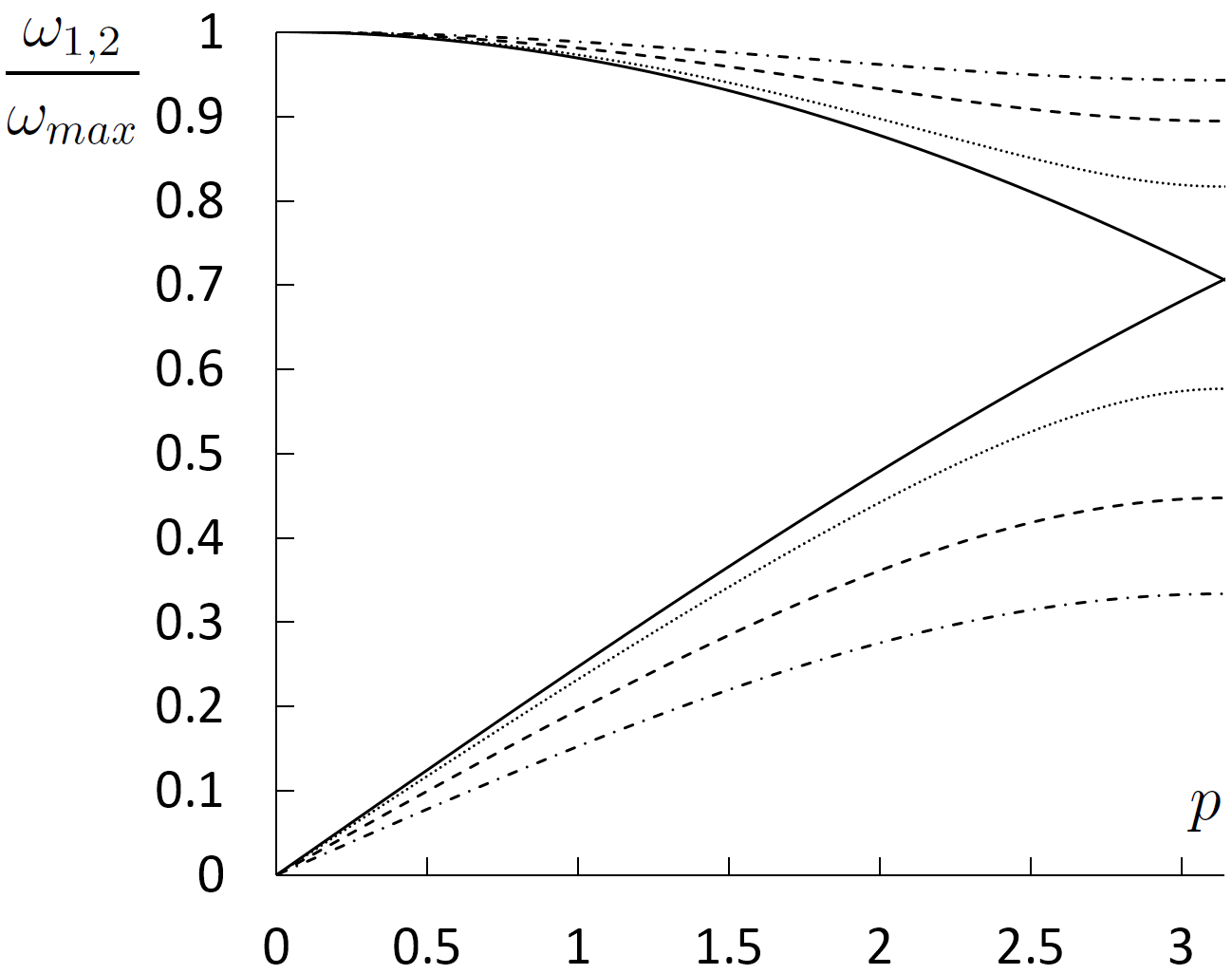
Refer to caption
Figure 3: Dispersion relation for a chain with alternating stiffnesses (m1=m2subscript𝑚1subscript𝑚2m_{1}=m_{2}). Curves correspond to different stiffness ratios: c1c2=1subscript𝑐1subscript𝑐21\frac{c_{1}}{c_{2}}=1 (solid line); 1212\frac{1}{2} (dots); 1414\frac{1}{4} (dashed line); 1818\frac{1}{8} (dash-dotted line).

We calculate matrix 𝐏𝐏\boldsymbol{\mathrm{P}}{}{} in equation (20). By definition, matrix 𝐏𝐏\boldsymbol{\mathrm{P}}{}{} consists of normalized eigenvectors of dynamical matrix 𝛀𝛀\mathbf{\Omega}. Eigenvectors 𝐝1,2\boldsymbol{\mathrm{d}}{}_{1,2}, corresponding to eigenvalues ω1,22superscriptsubscript𝜔122\omega_{1,2}^{2} (formula (40)), have form:

𝐝=1,2(1m1m2±(1m1m2)2+4|b|2m1m2;2bm1m2),b=c1+c2eipc1+c2.\boldsymbol{\mathrm{d}}{}_{1,2}=\left(1-\frac{m_{1}}{m_{2}}\pm\sqrt{\left(1-\frac{m_{1}}{m_{2}}\right)^{2}+4|b|^{2}\frac{m_{1}}{m_{2}}};-2b\sqrt{\frac{m_{1}}{m_{2}}}\right)^{\top},\qquad b=\frac{c_{1}+c_{2}e^{{\rm i}p}}{c_{1}+c_{2}}. (41)

Normalization of vectors 𝐝1,2\boldsymbol{\mathrm{d}}{}_{1,2} yields columns of matrix 𝐏𝐏\boldsymbol{\mathrm{P}}{}{}.

In the following sections, formulas (40), (41) are employed for description of temperature oscillations and calculation of equilibrium temperatures of sublattices.

5.3 Oscillations of kinetic temperature

In this section, we consider oscillations of kinetic temperature of the unit cell T=12(T11+T22)𝑇12subscript𝑇11subscript𝑇22T=\frac{1}{2}\left(T_{11}+T_{22}\right). The oscillations are caused by equilibration of kinetic and potential energies.

Initially particles have random velocities and zero displacements. Initial kinetic energies (temperatures) of sublattices are equal (T110=T220superscriptsubscript𝑇110superscriptsubscript𝑇220T_{11}^{0}=T_{22}^{0}). The oscillations of kinetic temperature are described by formula (23). In this case, the formula reads

T=T02+Tac+Top,Tac=T08π02πcos(2ω2(p)t)dp,Top=T08π02πcos(2ω1(p)t)dp,formulae-sequence𝑇subscript𝑇02subscript𝑇𝑎𝑐subscript𝑇𝑜𝑝formulae-sequencesubscript𝑇𝑎𝑐subscript𝑇08𝜋superscriptsubscript02𝜋2subscript𝜔2𝑝𝑡differential-d𝑝subscript𝑇𝑜𝑝subscript𝑇08𝜋superscriptsubscript02𝜋2subscript𝜔1𝑝𝑡differential-d𝑝\begin{array}[]{l}\displaystyle T=\frac{T_{0}}{2}+T_{ac}+T_{op},\quad T_{ac}=\frac{T_{0}}{8\pi}\int_{0}^{2\pi}\cos(2\omega_{2}(p)t){\rm d}p,\quad T_{op}=\frac{T_{0}}{8\pi}\int_{0}^{2\pi}\cos(2\omega_{1}(p)t){\rm d}p,\end{array} (42)

where T0=12(T110+T220)subscript𝑇012superscriptsubscript𝑇110superscriptsubscript𝑇220T_{0}=\frac{1}{2}\left(T_{11}^{0}+T_{22}^{0}\right) is initial kinetic temperature; dispersion relation ωj(p),j=1,2formulae-sequencesubscript𝜔𝑗𝑝𝑗12\omega_{j}(p),j=1,2 is given by formula (40). Contributions of acoustic and optical branches to temperature oscillations are given by integrals Tacsubscript𝑇𝑎𝑐T_{ac}, Topsubscript𝑇𝑜𝑝T_{op}.

Integrals in formula (42) are calculated numerically using Riemann sum approximation. Interval of integration is divided into 103superscript10310^{3} equal segments.

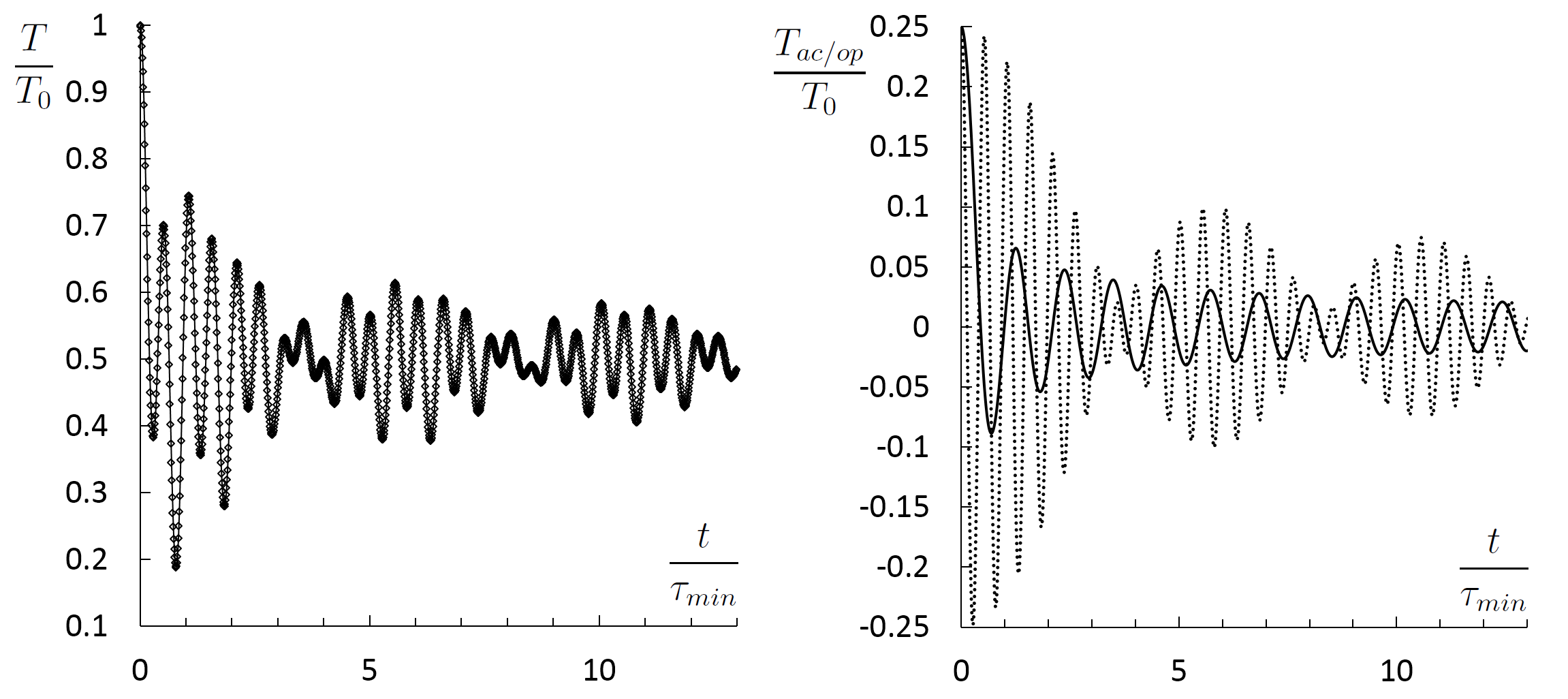
To check formula (42), we compare it with results of numerical solution of lattice dynamics equations (37). In simulations, the chain consists of 51055superscript1055\cdot 10^{5} particles under periodic boundary conditions. Numerical integration is carried out using symplectic leap-frog integrator with time-step 103τminsuperscript103subscript𝜏𝑚𝑖𝑛10^{-3}\tau_{min}, where τmin=2π/ωmaxsubscript𝜏𝑚𝑖𝑛2𝜋subscript𝜔𝑚𝑎𝑥\tau_{min}=2\pi/\omega_{max}, ωmaxsubscript𝜔𝑚𝑎𝑥\omega_{max} is defined by formula (40). During the simulation the total kinetic energy of the chain, proportional to kinetic temperature, is calculated. In this case, averaging over realizations is not necessary. Time dependence of temperature for m2/m1=4subscript𝑚2subscript𝑚14m_{2}/m_{1}=4 is shown in fig. 4A.

Refer to caption
Figure 4: A. Oscillations of kinetic temperature (m2=4m1subscript𝑚24subscript𝑚1m_{2}=4m_{1}, c1=c2subscript𝑐1subscript𝑐2c_{1}=c_{2}). Initial temperatures of sublattices are equal. Analytical solution (42) (solid line), and numerical solution (dots). B. Contribution of acoustic (Tacsubscript𝑇𝑎𝑐T_{ac}, solid line) and optical (Topsubscript𝑇𝑜𝑝T_{op}, dots) branches to oscillations of kinetic temperature (m2=4m1subscript𝑚24subscript𝑚1m_{2}=4m_{1}, c1=c2subscript𝑐1subscript𝑐2c_{1}=c_{2}).

It is seen that analytical solution (42) practically coincides with results of numerical integration of lattice dynamics equations.

Consider contributions Tacsubscript𝑇𝑎𝑐T_{ac}, Topsubscript𝑇𝑜𝑝T_{op} of two branches of dispersion relation to oscillations of kinetic temperature. Time dependencies of Tacsubscript𝑇𝑎𝑐T_{ac}, Topsubscript𝑇𝑜𝑝T_{op} for m2=4m1subscript𝑚24subscript𝑚1m_{2}=4m_{1}, c1=c2subscript𝑐1subscript𝑐2c_{1}=c_{2} are shown in fig. 4B. It is seen that contribution of optical branch has a form of beats (two close frequencies), while contribution of acoustic branch has one main frequency. Using the stationary phase method [16] it can be shown that characteristic frequencies of temperature oscillations belong to frequency spectrum of the chain. Group velocities, corresponding to these frequencies, are equal to zero. Figure 3 shows that group velocity of acoustic waves is equal to zero for p=π𝑝𝜋p=\pi, and group velocity of optical waves vanishes at p=0,p=πformulae-sequence𝑝0𝑝𝜋p=0,p=\pi. Then main frequencies of temperature oscillations are the following

ω1|p=0=ωmax,ω12|p=π=ωmax22(1+116m1m2c1c2(m1+m2)2(c1+c2)2),ω22|p=π=ωmax22(1116m1m2c1c2(m1+m2)2(c1+c2)2).formulae-sequenceevaluated-atsubscript𝜔1𝑝0subscript𝜔𝑚𝑎𝑥evaluated-atsuperscriptsubscript𝜔12𝑝𝜋superscriptsubscript𝜔𝑚𝑎𝑥221116subscript𝑚1subscript𝑚2subscript𝑐1subscript𝑐2superscriptsubscript𝑚1subscript𝑚22superscriptsubscript𝑐1subscript𝑐22evaluated-atsuperscriptsubscript𝜔22𝑝𝜋superscriptsubscript𝜔𝑚𝑎𝑥221116subscript𝑚1subscript𝑚2subscript𝑐1subscript𝑐2superscriptsubscript𝑚1subscript𝑚22superscriptsubscript𝑐1subscript𝑐22\begin{array}[]{l}\displaystyle\omega_{1}|_{p=0}=\omega_{max},\qquad\omega_{1}^{2}|_{p=\pi}=\frac{\omega_{max}^{2}}{2}\left(1+\sqrt{1-\frac{16m_{1}m_{2}c_{1}c_{2}}{(m_{1}+m_{2})^{2}(c_{1}+c_{2})^{2}}}\right),\\[11.38109pt] \displaystyle\omega_{2}^{2}|_{p=\pi}=\frac{\omega_{max}^{2}}{2}\left(1-\sqrt{1-\frac{16m_{1}m_{2}c_{1}c_{2}}{(m_{1}+m_{2})^{2}(c_{1}+c_{2})^{2}}}\right).\end{array} (43)

At large times, oscillations of kinetic temperature is represented as a sum of three harmonics with frequencies (43) and amplitudes, inversely proportional to t𝑡\sqrt{t}.

Difference between optical frequencies ω1|p=0evaluated-atsubscript𝜔1𝑝0\omega_{1}|_{p=0} and ω1|p=πevaluated-atsubscript𝜔1𝑝𝜋\omega_{1}|_{p=\pi} decreases with increasing mass ratio, therefore beats of kinetic temperature are observed (see fig. 4). Note that similar beats of temperature are observed in two-dimensional triangular lattice [58].

Consider influence of ratio between initial temperatures of sublattices T110superscriptsubscript𝑇110T_{11}^{0}, T220superscriptsubscript𝑇220T_{22}^{0} on temperature oscillations. The oscillations for two different cases, T1100,T220=0formulae-sequencesuperscriptsubscript𝑇1100superscriptsubscript𝑇2200T_{11}^{0}\neq 0,T_{22}^{0}=0 and T110=0,T2200formulae-sequencesuperscriptsubscript𝑇1100superscriptsubscript𝑇2200T_{11}^{0}=0,T_{22}^{0}\neq 0, are shown in fig. 5. It is seen that form of oscillations significantly depends on the ratio between T110superscriptsubscript𝑇110T_{11}^{0} and T220superscriptsubscript𝑇220T_{22}^{0}. In both cases, analytical results, obtained using formula (23), practically coincide with numerical solution of lattice dynamics equations.
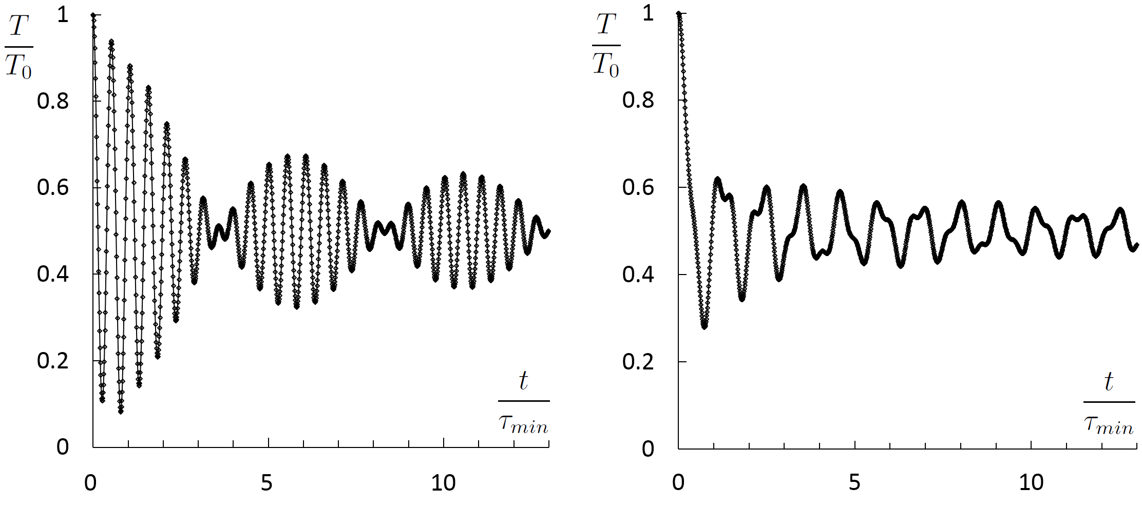
Refer to caption
Figure 5: Influence of initial temperatures of sublattices on temperature oscillations (m2=4m1subscript𝑚24subscript𝑚1m_{2}=4m_{1}, c1=c2subscript𝑐1subscript𝑐2c_{1}=c_{2}). Here T1100,T220=0formulae-sequencesuperscriptsubscript𝑇1100superscriptsubscript𝑇2200T_{11}^{0}\neq 0,T_{22}^{0}=0 (left) and T110=0,T2200formulae-sequencesuperscriptsubscript𝑇1100superscriptsubscript𝑇2200T_{11}^{0}=0,T_{22}^{0}\neq 0 (right). Formula (23) (line), and numerical solution of lattice dynamics equations (dots).

Thus temperature oscillations are accurately described by formula (23). Amplitude of the oscillations decay in time as181818This fact follows form the asymptotic analysis based on the stationary phase method [16]. 1/t1𝑡1/\sqrt{t}. Main frequencies of temperature oscillations belong to spectrum of the chain and correspond to zero group velocities. Form of oscillations significantly depends on initial distribution of energy between sublattices.

5.4 Redistribution of temperature between sublattices

In this section, we consider the case when initial temperatures of sublattices are not equal (T110T220superscriptsubscript𝑇110superscriptsubscript𝑇220T_{11}^{0}\neq T_{22}^{0}). Then temperature is redistributed between the sublattices.

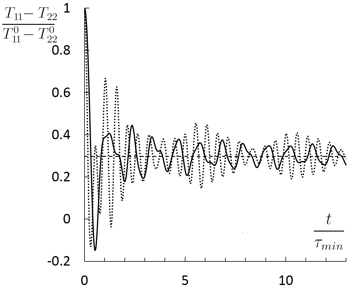
Numerical solution of equations of motion (37) shows that difference between temperatures of sublattices, T11T22subscript𝑇11subscript𝑇22T_{11}-T_{22}, tends to some equilibrium value. For example, behavior of T11T22subscript𝑇11subscript𝑇22T_{11}-T_{22} for m2=4m1subscript𝑚24subscript𝑚1m_{2}=4m_{1}, c1=c2subscript𝑐1subscript𝑐2c_{1}=c_{2} is shown in fig. 6. Two cases T1100,T220=0formulae-sequencesuperscriptsubscript𝑇1100superscriptsubscript𝑇2200T_{11}^{0}\neq 0,T_{22}^{0}=0 and T110=0,T2200formulae-sequencesuperscriptsubscript𝑇1100superscriptsubscript𝑇2200T_{11}^{0}=0,T_{22}^{0}\neq 0 are considered.

Refer to caption
Figure 6: Difference between temperatures of sublattices for T1100,T220=0formulae-sequencesuperscriptsubscript𝑇1100superscriptsubscript𝑇2200T_{11}^{0}\neq 0,T_{22}^{0}=0 (solid line), and T110=0,T2200formulae-sequencesuperscriptsubscript𝑇1100superscriptsubscript𝑇2200T_{11}^{0}=0,T_{22}^{0}\neq 0 (dots). Here m2=4m1subscript𝑚24subscript𝑚1m_{2}=4m_{1}, c1=c2subscript𝑐1subscript𝑐2c_{1}=c_{2}, T110,T220superscriptsubscript𝑇110superscriptsubscript𝑇220T_{11}^{0},T_{22}^{0} are initial temperatures of sublattices.

It is seen that in both cases difference between temperatures tends to the value 0.3(T110T220)0.3superscriptsubscript𝑇110superscriptsubscript𝑇2200.3(T_{11}^{0}-T_{22}^{0}), predicted by formula (45). Note that shape of curves for two initial conditions is different. Therefore the process of redistribution of temperature between sublattices depends on ratio between T110superscriptsubscript𝑇110T_{11}^{0} and T220superscriptsubscript𝑇220T_{22}^{0}.

We calculate the difference between temperatures of sublattices at thermal equilibrium using formula (25). Deviator of initial temperature matrix has form

dev𝐓=0T110T2202𝐈,𝐈=[1001].{\rm dev}\boldsymbol{\mathrm{T}}{}_{0}=\frac{T_{11}^{0}-T_{22}^{0}}{2}\boldsymbol{\mathrm{I}}{},\qquad\boldsymbol{\mathrm{I}}{}=\begin{bmatrix}1&0\\ 0&-1\end{bmatrix}. (44)

Substituting (44) into formula (25), yields:

𝐓=eq14(T110+T220)𝐄+T110T2204π02π𝐏diag(𝐏𝐈𝐏)𝐏dp.\boldsymbol{\mathrm{T}}{}_{eq}=\frac{1}{4}\left(T_{11}^{0}+T_{22}^{0}\right)\boldsymbol{\mathrm{E}}{}+\frac{T_{11}^{0}-T_{22}^{0}}{4\pi}\int_{0}^{2\pi}\boldsymbol{\mathrm{P}}{}{}{\rm diag}\left(\boldsymbol{\mathrm{P}}{}{}^{*{\top}}\boldsymbol{\mathrm{I}}{}\boldsymbol{\mathrm{P}}{}{}\right)\boldsymbol{\mathrm{P}}{}{}^{*{\top}}{\rm d}p. (45)

Matrix 𝐏𝐏\boldsymbol{\mathrm{P}}{}{} is given by formula (41). Formula (45) yields equilibrium temperatures of sublattices. Integral in formula (45) is calculated numerically using Riemann sum approximation. Interval of integration is divided into 103superscript10310^{3} equal segments.

Consider the case of equal masses m1=m2subscript𝑚1subscript𝑚2m_{1}=m_{2}. Using formula (41) it can be shown that diagonal elements of matrix 𝐏𝐈𝐏𝐏superscript𝐈𝐏absenttop\boldsymbol{\mathrm{P}}{}{}^{*{\top}}\boldsymbol{\mathrm{I}}{}\boldsymbol{\mathrm{P}}{}{} are equal to zero. Then from formula (45) it follows that for m1=m2subscript𝑚1subscript𝑚2m_{1}=m_{2} and arbitrary c1/c2subscript𝑐1subscript𝑐2c_{1}/c_{2} temperatures of sublattices at thermal equilibrium are equal.

To check formula (45), we compare it with results of numerical solution of lattice dynamics equations (37). The chain consists of 104superscript10410^{4} particles under periodic boundary conditions. We limit ourselves by the following range of parameters:  m1/m2[0;1]subscript𝑚1subscript𝑚201m_{1}/m_{2}\in[0;1] and c1/c2[0;1]subscript𝑐1subscript𝑐201c_{1}/c_{2}\in[0;1]. Numerical integration is carried out with time step 103τsuperscript103subscript𝜏10^{-3}\tau_{*}, where τ=c1+c2m1subscript𝜏subscript𝑐1subscript𝑐2subscript𝑚1\tau_{*}=\sqrt{\frac{c_{1}+c_{2}}{m_{1}}}. Initially particles have random velocities such that one of sublattices has zero temperature. During the simulation temperatures of sublattices are calculated. Equilibrium temperatures are computed by averaging corresponding kinetic energies over time interval [tmax/4;tmax]subscript𝑡𝑚𝑎𝑥4subscript𝑡𝑚𝑎𝑥[t_{max}/4;t_{max}], where tmaxsubscript𝑡𝑚𝑎𝑥t_{max} is the total simulation time. Reasonable accuracy is achieved for tmax=102τsubscript𝑡𝑚𝑎𝑥superscript102subscript𝜏t_{max}=10^{2}\tau_{*}.

Refer to caption
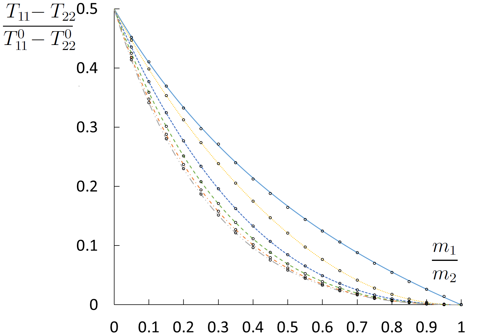
Figure 7: Difference between equilibrium temperatures of sublattices for a diatomic chain. Here T110,T220superscriptsubscript𝑇110superscriptsubscript𝑇220T_{11}^{0},T_{22}^{0} are initial temperatures of sublattices. Curves are calculated using formula (45) for c1c2=1subscript𝑐1subscript𝑐21\frac{c_{1}}{c_{2}}=1 (solid line); 1212\frac{1}{2} (doted line); 1414\frac{1}{4} (short dashed line); 1818\frac{1}{8} (dashed line); 116116\frac{1}{16} (dash-dotted line); 132132\frac{1}{32} (dash-double doted line). Circles correspond to results of numerical integration of equations of motion (37).

Equilibrium difference between temperatures of sublattices for different mass and stiffness ratios is shown in fig. 7. It is seen that for any given mass ratio, difference between temperatures decreases with decreasing c1/c2subscript𝑐1subscript𝑐2c_{1}/c_{2} and tends to a limiting value corresponding to the case c1/c20subscript𝑐1subscript𝑐20c_{1}/c_{2}\rightarrow 0. In particular, results for c2=64c1subscript𝑐264subscript𝑐1c_{2}=64c_{1} and c2=32c1subscript𝑐232subscript𝑐1c_{2}=32c_{1} are practically indistinguishable.

Thus for the given system, equilibrium temperatures of sublattices are equal if either 1) initial temperatures are equal T110=T220superscriptsubscript𝑇110superscriptsubscript𝑇220T_{11}^{0}=T_{22}^{0} or 2) masses are equal m1=m2subscript𝑚1subscript𝑚2m_{1}=m_{2} and stiffness ratio is arbitrary. In general, equilibrium temperatures of sublattices are different. Their values are accurately determined by formula (45).

Remark. For equal stiffnesses c1=c2subscript𝑐1subscript𝑐2c_{1}=c_{2}, equation (37) is also valid for transverse vibrations of a stretched diatomic chain. In this case, the stiffness is determined by magnitude of stretching force. Therefore all results obtained in this section can be used in the case of transverse vibrations.

Remark. Our results may serve for better understanding of heat transfer in diatomic chains. In papers [32, 61], stationary heat transfer in diatomic chains connecting two thermal reservoirs with different temperatures was investigated. In paper [9] it was shown that for m1m2subscript𝑚1subscript𝑚2m_{1}\neq m_{2} temperatures of sublattices were different (temperature profile was not smooth), while in paper [61] temperatures of sublattices for m1=m2subscript𝑚1subscript𝑚2m_{1}=m_{2} and c1c2subscript𝑐1subscript𝑐2c_{1}\neq c_{2} were practically equal. We suppose that these results can be explained using formula (45), which shows that equilibrium temperatures of sublattices are equal only for m1=m2subscript𝑚1subscript𝑚2m_{1}=m_{2}.

6 Example. Graphene lattice (out-of-plane motions)

6.1 Equations of motion

In this section, we consider approach to thermal equilibrium in hexagonal lattice (see fig. 8). Only out-of-plane vibrations are considered. The given model describes out-of-plane vibrations of a stretched graphene sheet [3, 6, 21]. In-plane vibrations can be considered separately, since in harmonic approximation in-plane and out-of-plane vibrations are decoupled.
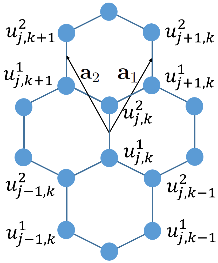
Refer to caption
Figure 8: Numbering of unit cells and basis vectors 𝐚1\boldsymbol{\mathrm{a}}{}_{1}, 𝐚2\boldsymbol{\mathrm{a}}{}_{2} for graphene lattice. Particles move along the normal to lattice plane.

Elementary cells, containing two particles each, are numbered by a pair of indices j,k𝑗𝑘j,k (see fig.8). Basis vectors 𝐚1\boldsymbol{\mathrm{a}}{}_{1} and 𝐚2\boldsymbol{\mathrm{a}}{}_{2} for graphene have form:

𝐚=13a2(𝐢+3𝐣),𝐚=23a2(3𝐣𝐢),\boldsymbol{\mathrm{a}}{}_{1}=\frac{\sqrt{3}a}{2}\left(\boldsymbol{\mathrm{i}}{}+\sqrt{3}\boldsymbol{\mathrm{j}}{}\right),\qquad\boldsymbol{\mathrm{a}}{}_{2}=\frac{\sqrt{3}a}{2}\left(\sqrt{3}\boldsymbol{\mathrm{j}}{}-\boldsymbol{\mathrm{i}}{}\right), (46)

where 𝐢,𝐣𝐢𝐣\boldsymbol{\mathrm{i}}{},\boldsymbol{\mathrm{j}}{} are Cartesian unit vectors; in fig. 8 vector 𝐢𝐢\boldsymbol{\mathrm{i}}{} is horizontal. Vector 𝐚1\boldsymbol{\mathrm{a}}{}_{1} connects centers of cells j,k𝑗𝑘j,k and j+1,k𝑗1𝑘j+1,k. Vector 𝐚2\boldsymbol{\mathrm{a}}{}_{2} connects centers of cells j,k𝑗𝑘j,k and j,k+1𝑗𝑘1j,k+1. Position vector of cell j,k𝑗𝑘j,k has form:

𝐱=j,k3a(j𝐞+1k𝐞)2,𝐞=1𝐚1|𝐚|1,𝐞=2𝐚2|𝐚|2.\boldsymbol{\mathrm{x}}{}_{j,k}=\sqrt{3}a\left(j\boldsymbol{\mathrm{e}}{}_{1}+k\boldsymbol{\mathrm{e}}{}_{2}\right),\qquad\boldsymbol{\mathrm{e}}{}_{1}=\frac{\boldsymbol{\mathrm{a}}{}_{1}}{|\boldsymbol{\mathrm{a}}{}_{1}|},\qquad\boldsymbol{\mathrm{e}}{}_{2}=\frac{\boldsymbol{\mathrm{a}}{}_{2}}{|\boldsymbol{\mathrm{a}}{}_{2}|}. (47)

Each particle has one degree of freedom (displacement normal to lattice plane). Displacements of a unit cell j,k𝑗𝑘j,k form a column:

𝐮=j,k𝐮(𝐱)j,k=(uj,k1,uj,k2),\boldsymbol{\mathrm{u}}{}_{j,k}=\boldsymbol{\mathrm{u}}{}(\boldsymbol{\mathrm{x}}{}_{j,k})=\left(u^{1}_{j,k},u^{2}_{j,k}\right)^{\top}, (48)

where uj,k1,uj,k2subscriptsuperscript𝑢1𝑗𝑘subscriptsuperscript𝑢2𝑗𝑘u^{1}_{j,k},u^{2}_{j,k} are displacements of two sublattices.

Consider equations of motion of unit cell j,k𝑗𝑘j,k. Each particle is connected with three nearest neighbors by linear springs (solid lines in fig. 8). Equilibrium length of the spring is less than initial distance between particles, i.e. the graphene sheet is uniformly stretched 191919In the absence of stretching, out-of-plane vibrations are essentially nonlinear. Various nonlinear effects in unstrained graphene are considered e.g. in papers [4, 34].. Stiffness of the spring, determined by stretching force, is denoted by c𝑐c. Then equations of motion have form

𝐌𝐮¨j,k=𝐂𝐮1+j+1,k𝐂𝐮1+j1,k𝐂𝐮0+j,k𝐂𝐮2+j,k+1𝐂𝐮2,j,k1𝐂=0[3ccc3c],𝐂=1𝐂=2[00c0],𝐌=[m00m].\begin{array}[]{l}\boldsymbol{\mathrm{M}}{}{}\ddot{\boldsymbol{\mathrm{u}}{}}_{j,k}=\boldsymbol{\mathrm{C}}{}_{1}\boldsymbol{\mathrm{u}}{}_{j+1,k}+\boldsymbol{\mathrm{C}}{}_{-1}\boldsymbol{\mathrm{u}}{}_{j-1,k}+\boldsymbol{\mathrm{C}}{}_{0}\boldsymbol{\mathrm{u}}{}_{j,k}+\boldsymbol{\mathrm{C}}{}_{2}\boldsymbol{\mathrm{u}}{}_{j,k+1}+\boldsymbol{\mathrm{C}}{}_{-2}\boldsymbol{\mathrm{u}}{}_{j,k-1},\\[11.38109pt] \boldsymbol{\mathrm{C}}{}_{0}=\begin{bmatrix}-3c&c\\ c&-3c\end{bmatrix},\quad\boldsymbol{\mathrm{C}}{}_{1}=\boldsymbol{\mathrm{C}}{}_{2}=\begin{bmatrix}0&0\\ c&0\end{bmatrix},\quad\boldsymbol{\mathrm{M}}{}{}=\begin{bmatrix}m&0\\ 0&m\end{bmatrix}.\end{array} (49)

Here 𝐂=1𝐂1\boldsymbol{\mathrm{C}}{}_{-1}=\boldsymbol{\mathrm{C}}{}_{1}^{\top}, 𝐂=2𝐂2\boldsymbol{\mathrm{C}}{}_{-2}=\boldsymbol{\mathrm{C}}{}_{2}^{\top}; m𝑚m is particle mass.

Initially particles have random velocities and zero displacements. Velocities are chosen such that initial temperatures of sublattices are different (T110T220superscriptsubscript𝑇110superscriptsubscript𝑇220T_{11}^{0}\neq T_{22}^{0}). Velocities of different sublattices are uncorrelated, i.e. u˙j,k1u˙j,k2=0delimited-⟨⟩subscriptsuperscript˙𝑢1𝑗𝑘subscriptsuperscript˙𝑢2𝑗𝑘0\Bigl{\langle}{\dot{u}^{1}_{j,k}\dot{u}^{2}_{j,k}}\Bigr{\rangle}=0. Then initial temperature matrix, 𝐓0\boldsymbol{\mathrm{T}}{}_{0}, has form:

𝐓=0[T11000T220],kBT110=m(u˙j,k1)2,kBT220=m(u˙j,k2)2.\begin{array}[]{l}\displaystyle\boldsymbol{\mathrm{T}}{}_{0}=\begin{bmatrix}T_{11}^{0}&0\\ 0&T_{22}^{0}\end{bmatrix},\qquad k_{B}T_{11}^{0}=m\Bigl{\langle}{\left(\dot{u}^{1}_{j,k}\right)^{2}}\Bigr{\rangle},\qquad k_{B}T_{22}^{0}=m\Bigl{\langle}{\left(\dot{u}^{2}_{j,k}\right)^{2}}\Bigr{\rangle}.\end{array} (50)

Here velocities are calculated at t=0𝑡0t=0. Initial temperature distribution is spatially uniform, i.e. T110,T220superscriptsubscript𝑇110superscriptsubscript𝑇220T_{11}^{0},T_{22}^{0} are independent on j,k𝑗𝑘j,k. Further we consider time evolution of temperatures of sublattices, equal to diagonal elements of the temperature matrix T11subscript𝑇11T_{11}, T22subscript𝑇22T_{22}.

6.2 Dispersion relation

Evolution of temperature matrix during approach to thermal equilibrium is described by formula (20). In this section, we calculate the dispersion relation and matrix 𝐏𝐏\boldsymbol{\mathrm{P}}{}{} included in this formula.

We calculate dynamical matrix 𝛀𝛀\mathbf{\Omega} using formula (16). Substituting expressions (49) for matrixes 𝐂α\boldsymbol{\mathrm{C}}{}_{\alpha}, α=0;±1;±2𝛼0plus-or-minus1plus-or-minus2\alpha=0;\pm 1;\pm 2 into formula (16), we obtain:

𝛀=ω2[31eip1eip21eip1eip23],p1=𝐤𝐚,1p2=𝐤𝐚,2\begin{array}[]{l}\displaystyle\mathbf{\Omega}=\omega_{*}^{2}\begin{bmatrix}3&-1-e^{-{\rm i}p_{1}}-e^{-{\rm i}p_{2}}\\ -1-e^{{\rm i}p_{1}}-e^{{\rm i}p_{2}}&3\end{bmatrix},\qquad p_{1}=\boldsymbol{\mathrm{k}}{}\cdot\boldsymbol{\mathrm{a}}{}_{1},\quad p_{2}=\boldsymbol{\mathrm{k}}{}\cdot\boldsymbol{\mathrm{a}}{}_{2},\end{array} (51)

where 𝐤𝐤\boldsymbol{\mathrm{k}}{} is wave-vector; ω2=cmsuperscriptsubscript𝜔2𝑐𝑚\omega_{*}^{2}=\frac{c}{m}; p1,p2[0;2π]subscript𝑝1subscript𝑝202𝜋p_{1},p_{2}\in[0;2\pi] are dimensionless components of the wave vector.

Eigenvalues ω12,ω22superscriptsubscript𝜔12superscriptsubscript𝜔22\omega_{1}^{2},\omega_{2}^{2} of matrix 𝛀𝛀\mathbf{\Omega} determine dispersion relation for the lattice. Solution of the eigenvalue problem yields:

ω1,22=ω2(3±3+2(cosp1+cosp2+cos(p1p2))),superscriptsubscript𝜔122superscriptsubscript𝜔2plus-or-minus332subscript𝑝1subscript𝑝2subscript𝑝1subscript𝑝2\omega_{1,2}^{2}=\omega_{*}^{2}\left(3\pm\sqrt{3+2\left(\cos p_{1}+\cos p_{2}+\cos\left(p_{1}-p_{2}\right)\right)}\right), (52)

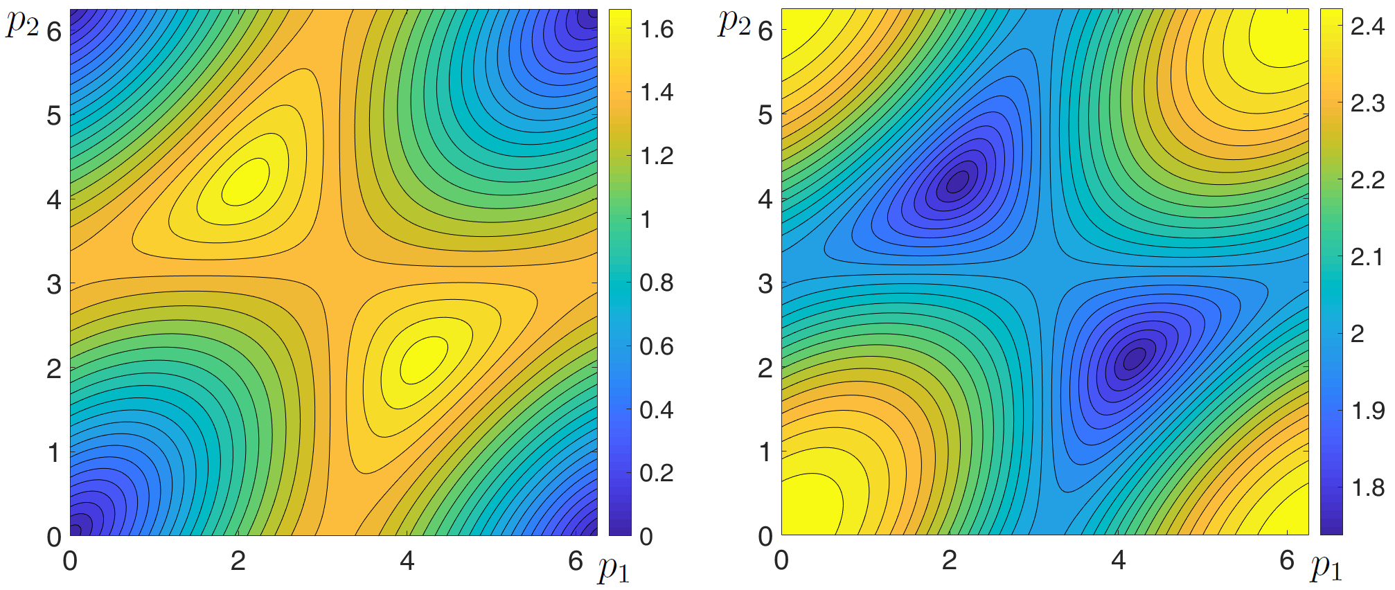
where index 111 corresponds to plus sign. Functions ω1(p1,p2)subscript𝜔1subscript𝑝1subscript𝑝2\omega_{1}(p_{1},p_{2}), ω2(p1,p2)subscript𝜔2subscript𝑝1subscript𝑝2\omega_{2}(p_{1},p_{2}) are referred to as optical and acoustic dispersion surfaces respectively (see fig. 9).
Refer to caption
Figure 9: Acoustic (ω2(p1,p2)/ωsubscript𝜔2subscript𝑝1subscript𝑝2subscript𝜔\omega_{2}(p_{1},p_{2})/\omega_{*}, left) and optical (ω1(p1,p2)/ωsubscript𝜔1subscript𝑝1subscript𝑝2subscript𝜔\omega_{1}(p_{1},p_{2})/\omega_{*}, right) dispersion surfaces (52) for out-of-plane vibrations of graphene.

Eigenvectors of matrix 𝛀𝛀\mathbf{\Omega} are columns of matrix 𝐏𝐏\boldsymbol{\mathrm{P}}{}{}:

𝐏=1|b|2+b2[|b||b|bb],b=1+eip1+eip2.formulae-sequence𝐏1superscript𝑏2superscript𝑏2matrix𝑏𝑏𝑏𝑏𝑏1superscript𝑒isubscript𝑝1superscript𝑒isubscript𝑝2\boldsymbol{\mathrm{P}}{}{}=\frac{1}{\sqrt{|b|^{2}+b^{2}}}\begin{bmatrix}|b|&|b|\\ -b&b\end{bmatrix},\qquad b=1+e^{{\rm i}p_{1}}+e^{{\rm i}p_{2}}. (53)

In the following sections, formulas (51), (52), (53) are employed for description of temperature oscillations and calculation of equilibrium temperatures of sublattices.

6.3 Oscillations of kinetic temperature

In this section, we consider oscillations of kinetic temperature of the unit cell T=12(T11+T22)𝑇12subscript𝑇11subscript𝑇22T=\frac{1}{2}(T_{11}+T_{22}) in graphene.

In general, the oscillations are described by formula (22). Using formulas (50), (53) it can be shown that diagonal elements of matrix 𝐏dev𝐓𝐏0𝐏superscriptdevabsenttop𝐓subscript𝐏0\boldsymbol{\mathrm{P}}{}{}^{*{\top}}{\rm dev}\boldsymbol{\mathrm{T}}{}_{0}\boldsymbol{\mathrm{P}}{}{} are equal to zero. Then from formula (22) it follows that temperature oscillations are independent of the ratio between temperatures of sublattices T110superscriptsubscript𝑇110T_{11}^{0} and T220superscriptsubscript𝑇220T_{22}^{0}. Then formula (23) can be used:

T=T02+Tac+Top,Tac=T016π202π02πcos(2ω2(p1,p2)t)dp1dp2,Top=T016π202π02πcos(2ω1(p1,p2)t)dp1dp2,formulae-sequence𝑇subscript𝑇02subscript𝑇𝑎𝑐subscript𝑇𝑜𝑝subscript𝑇𝑎𝑐subscript𝑇016superscript𝜋2superscriptsubscript02𝜋superscriptsubscript02𝜋2subscript𝜔2subscript𝑝1subscript𝑝2𝑡differential-dsubscript𝑝1differential-dsubscript𝑝2subscript𝑇𝑜𝑝subscript𝑇016superscript𝜋2superscriptsubscript02𝜋superscriptsubscript02𝜋2subscript𝜔1subscript𝑝1subscript𝑝2𝑡differential-dsubscript𝑝1differential-dsubscript𝑝2\begin{array}[]{l}\displaystyle T=\frac{T_{0}}{2}+T_{ac}+T_{op},\qquad T_{ac}=\frac{T_{0}}{16\pi^{2}}\int_{0}^{2\pi}\int_{0}^{2\pi}\cos(2\omega_{2}(p_{1},p_{2})t){\rm d}p_{1}{\rm d}p_{2},\\[11.38109pt] \displaystyle T_{op}=\frac{T_{0}}{16\pi^{2}}\int_{0}^{2\pi}\int_{0}^{2\pi}\cos(2\omega_{1}(p_{1},p_{2})t){\rm d}p_{1}{\rm d}p_{2},\end{array} (54)

where T0=12(T110+T220)subscript𝑇012superscriptsubscript𝑇110superscriptsubscript𝑇220T_{0}=\frac{1}{2}\left(T_{11}^{0}+T_{22}^{0}\right) is initial kinetic temperature; functions ω1,2(p1,p2)subscript𝜔12subscript𝑝1subscript𝑝2\omega_{1,2}(p_{1},p_{2}) are given by formula (52). In further calculations, integrals in formula (54) are evaluated using Riemann sum approximation. Integration area is divided into 400×400400400400\times 400 equal square elements.

To check formula (54), we compare it with results of numerical solution of lattice dynamics equations (49). In our simulations, graphene sheet contains 103×103superscript103superscript10310^{3}\times 10^{3} unit cells under periodic boundary conditions. Numerical integration is carried out with time-step 5103τ5superscript103subscript𝜏5\cdot 10^{-3}\tau_{*}, where τ=2π/ωsubscript𝜏2𝜋subscript𝜔\tau_{*}=2\pi/\omega_{*}. During the simulation the total kinetic energy of the lattice, proportional to kinetic temperature, is calculated. In this case, averaging over realizations is not necessary. Time dependence of temperature is presented in fig. 10A.
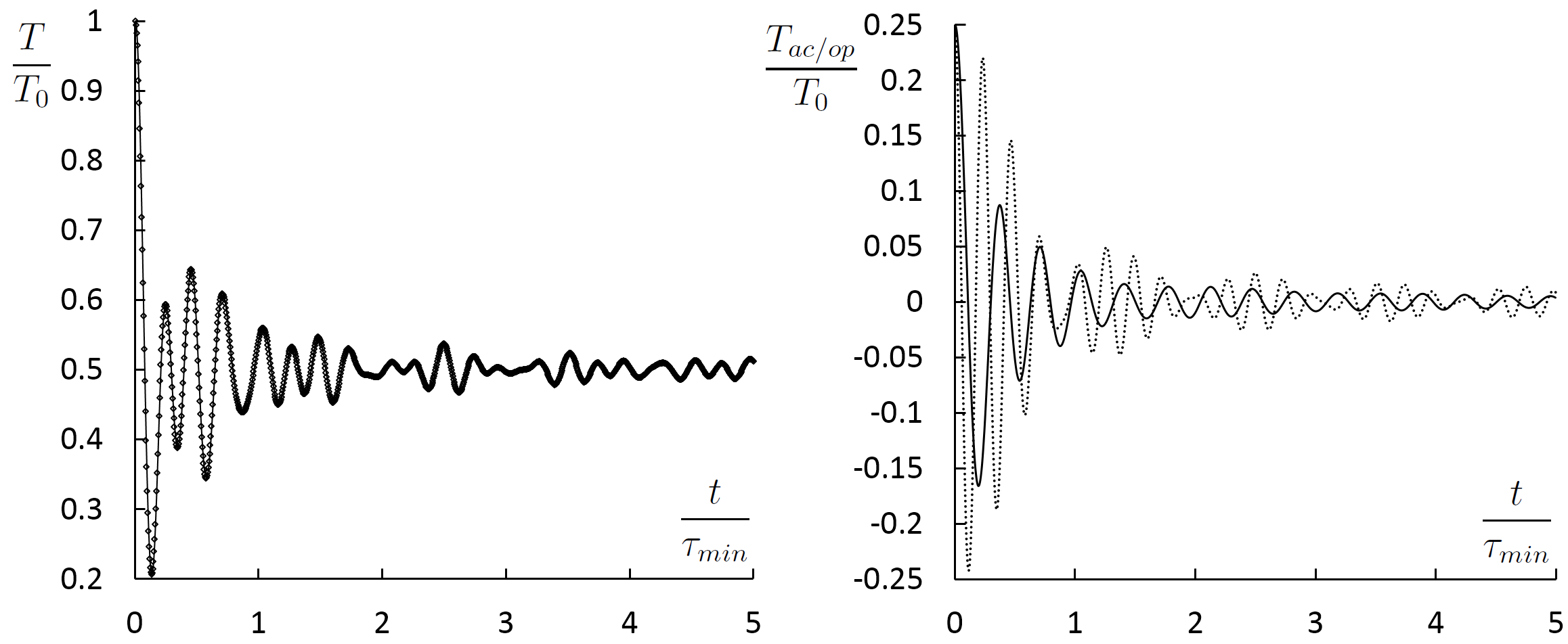
Refer to caption
Figure 10: A. Oscillations of kinetic temperature in graphene sheet with random initial velocities and zero displacements. Numerical solution of equations of motion (49) (dots) and analytical solution (54) (line). B. Contribution of acoustic (Tacsubscript𝑇𝑎𝑐T_{ac}, solid line) and optical (Topsubscript𝑇𝑜𝑝T_{op}, dotted line) dispersion surfaces to temperature oscillations in graphene.

The figure shows that formula (54) accurately describes temperature oscillations. Calculations with different initial temperatures of sublattices (T110T220superscriptsubscript𝑇110superscriptsubscript𝑇220T_{11}^{0}\neq T_{22}^{0}) confirm out conclusion that the ratio of these temperatures do not influence the behavior of T𝑇T.

Contributions of acoustic and optical dispersion surfaces to temperature oscillations are shown in fig. 10B. The contributions are given by integrals Tacsubscript𝑇𝑎𝑐T_{ac} and Topsubscript𝑇𝑜𝑝T_{op} (formula (54)). It is seen that oscillations corresponding to optical dispersion surface has two main frequencies, while oscillations corresponding to acoustic surface has only one main frequency. The frequencies can be calculated using asymptotic analysis of integrals (54) at large t𝑡t using the stationary phase method [16]. This investigation is beyond the scope of the present paper. Similar investigation for two-dimensional triangular lattice is carried out in paper [58].

Thus oscillations of kinetic temperature are accurately described by formula (54). Amplitude of these oscillations decays in time as 1/t1𝑡1/t. Formula (54) is valid for an arbitrary ratio of initial temperatures of sublattices.

6.4 Redistribution of temperature between sublattices

In this section, we consider redistribution of kinetic temperature between sublattices in graphene in the case T110T220superscriptsubscript𝑇110superscriptsubscript𝑇220T_{11}^{0}\neq T_{22}^{0}.

Equilibrium temperatures of sublattices are calculated using formula (25). Corresponding expression for initial temperature matrix is given by formula (50). In the previous section, it is mentioned that for graphene, matrix 𝐏dev𝐓0𝐏𝐏superscriptdevabsenttopsubscript𝐓0𝐏\boldsymbol{\mathrm{P}}{}{}^{*{\top}}{\rm dev}{\boldsymbol{\mathrm{T}}{}}_{0}\boldsymbol{\mathrm{P}}{}{} in formula (25) has zero diagonal elements. Then from formula (25) it follows that dev𝐓=eq0{\rm dev}\boldsymbol{\mathrm{T}}{}_{eq}=0, i.e. temperatures of sublattices equilibrate.

To check this fact, consider numerical solution of equations of motion (49). Periodic cell containing 103×103superscript103superscript10310^{3}\times 10^{3} unit cells is used. Initially particles of one sublattice have random velocities, while particles of another sublattice are motionless. Initial displacements are equal to zero. Numerical integration is carried with time step 5103τ5superscript103subscript𝜏5\cdot 10^{-3}\tau_{*}, where τ=2π/ωsubscript𝜏2𝜋subscript𝜔\tau_{*}=2\pi/\omega_{*}. Time evolution of temperature difference, T11T22subscript𝑇11subscript𝑇22T_{11}-T_{22}, is shown in fig. 11.

Refer to caption
Figure 11: Redistribution of kinetic temperatures between sublattices in graphene (numerical solution of lattice dynamics equations (49)).

The figure shows beats of difference between temperatures of sublattices. The amplitude of beats decays in time as 1/t1𝑡1/t.

Thus at large times, temperatures of sublattices in graphene become equal.

7 Conclusions

An analytical description of approach to thermal equilibrium in infinite harmonic crystals with complex (polyatomic) lattice was presented.

Initially the crystal is in a nonequilibrium state such that kinetic and potential energies are not equal. The crystal tends to thermal equilibrium, i.e. to a state in which temperatures, corresponding to different degrees of freedom of the unit cell, are constant in time. Approach to thermal equilibrium is accompanied by oscillations of the temperatures exactly described by formula (20). The oscillations are caused by two physical processes: 1) equilibration of kinetic and potential energies, and 2) redistribution of kinetic energy (temperature) among degrees of freedom of the unit cell. In d𝑑d-dimensional crystal, amplitude of the oscillations decays in time as 1/td21superscript𝑡𝑑21/t^{\frac{d}{2}}.

At large times, kinetic and potential energies equilibrate. Kinetic energy is redistributed between degrees of freedom of the unit cell. Equilibrium values of kinetic temperatures, corresponding to different degrees of freedom of the unit cell, are related with initial conditions by the non-equipartition theorem (formulas (25), (34)). The theorem shows that these kinetic temperatures are equal at thermal equilibrium if their initial values are equal. If initial kinetic temperatures are different then they are usually different at equilibrium, except for some lattices. For example, it is shown that in diatomic chain with alternating stiffnesses (equal masses) and graphene lattice performing out-of-plane motions the equilibrium values of the kinetic temperatures are equal.

Our analytical results are exact in the case of spatially uniform distribution of kinetic temperatures. In the case of nonuniform temperature distribution, ballistic heat transfer should be considered along with transient processes described above. However the heat transfer is much slower than the transient processes [19, 38, 42, 56]. Therefore at small times, the crystal locally almost achieve thermal equilibrium. This almost equilibrium state slowly changes due to ballistic heat transfer. Therefore our results can be used for description of fast local transition to thermal equilibrium in nonuniformly heated crystals.

In the present paper, anharmonic effects were neglected. Anharmonicity leads, in particular, to exchange of energy between normal modes. In this case, temperatures, corresponding to different degrees of freedom of the unit cell, tend to equal equilibrium values. However in papers [5, 41, 49], it is shown that, at least in the case of small anharmonicity, the exchange between normal modes is significantly slower than transient thermal processes described above. Therefore at small times, transient thermal processes are well described by harmonic approximation.

8 Acknowledgements

The author is deeply grateful to A.M. Krivtsov, S.V. Dmitriev, M.A. Guzev, D.A. Indeitsev, E.A. Ivanova, S.N. Gavrilov, I.E. Berinskii and A.S. Murachev for useful discussions. The work was financially supported by the Russian Science Foundation under grant No. 17-71-10213.

9 Appendix I. Equation for the generalized energies

In this appendix, we show that generalized kinetic energy (𝐊𝐊\boldsymbol{\mathrm{K}}{}{}), generalized potential energy (𝐏𝐏\boldsymbol{\mathrm{P}}{}{}), generalized Hamiltonian (𝐇𝐇\boldsymbol{\mathrm{H}}{}), and generalized Lagrangian (𝐋𝐋\boldsymbol{\mathrm{L}}{}) satisfy differential-difference equation (10).

We introduce matrix, 𝐙𝐙\boldsymbol{\mathrm{Z}}{}, consisting of covariances of particle accelerations:

𝐙=12𝐌𝐮¨(𝐱)𝐮¨(𝐲)12𝐌.12\boldsymbol{\mathrm{Z}}{}=\frac{1}{2}\boldsymbol{\mathrm{M}}{}{}^{\frac{1}{2}}\Bigl{\langle}{\ddot{\boldsymbol{\mathrm{u}}{}}(\boldsymbol{\mathrm{x}}{})\ddot{\boldsymbol{\mathrm{u}}{}}(\boldsymbol{\mathrm{y}}{})^{\top}}\Bigr{\rangle}\boldsymbol{\mathrm{M}}{}{}^{\frac{1}{2}}. (55)

Calculation of the second time derivatives of 𝐊𝐊\boldsymbol{\mathrm{K}}{}{} and 𝐙𝐙\boldsymbol{\mathrm{Z}}{} taking into account equations of motion, yields:

𝐊¨=𝓛𝐊x+𝐊𝓛+y2𝐙,𝐙¨=𝓛𝐙x+𝐙𝓛+y2𝓛𝐊x𝓛,y𝓛𝐊x=α𝐌𝐂12𝐌α𝐊12(𝐱+𝐚,α𝐲),𝐊𝓛=yTα𝐊(𝐱,𝐲𝐚)α𝐌𝐂12𝐌α.12\begin{array}[]{l}\ddot{\boldsymbol{\mathrm{K}}{}{}}=\boldsymbol{\mathrm{\cal{L}}}{}_{x}\boldsymbol{\mathrm{K}}{}{}+\boldsymbol{\mathrm{K}}{}{}\boldsymbol{\mathrm{\cal{L}}}{}_{y}^{\top}+2\boldsymbol{\mathrm{Z}}{},\qquad\ddot{\boldsymbol{\mathrm{Z}}{}}=\boldsymbol{\mathrm{\cal{L}}}{}_{x}\boldsymbol{\mathrm{Z}}{}+\boldsymbol{\mathrm{Z}}{}\boldsymbol{\mathrm{\cal{L}}}{}_{y}^{\top}+2\boldsymbol{\mathrm{\cal{L}}}{}_{x}\boldsymbol{\mathrm{K}}{}{}\boldsymbol{\mathrm{\cal{L}}}{}_{y}^{\top},\\[11.38109pt] \displaystyle\boldsymbol{\mathrm{\cal{L}}}{}_{x}\boldsymbol{\mathrm{K}}{}{}=\sum_{\alpha}\boldsymbol{\mathrm{M}}{}{}^{-\frac{1}{2}}\boldsymbol{\mathrm{C}}{}_{\alpha}\boldsymbol{\mathrm{M}}{}{}^{-\frac{1}{2}}\boldsymbol{\mathrm{K}}{}{}\left(\boldsymbol{\mathrm{x}}{}+\boldsymbol{\mathrm{a}}{}_{\alpha},\boldsymbol{\mathrm{y}}{}\right),\quad\boldsymbol{\mathrm{K}}{}{}\boldsymbol{\mathrm{\cal{L}}}{}_{y}^{\rm T}=\sum_{\alpha}\boldsymbol{\mathrm{K}}{}{}\left(\boldsymbol{\mathrm{x}}{},\boldsymbol{\mathrm{y}}{}-\boldsymbol{\mathrm{a}}{}_{\alpha}\right)\boldsymbol{\mathrm{M}}{}{}^{-\frac{1}{2}}\boldsymbol{\mathrm{C}}{}_{\alpha}\boldsymbol{\mathrm{M}}{}{}^{-\frac{1}{2}}.\end{array} (56)

Excluding 𝐙𝐙\boldsymbol{\mathrm{Z}}{} from this system of equations, we obtain

𝐊˙˙˙˙2(𝓛𝐊¨x+𝐊¨𝓛)y+𝓛𝐊x22𝓛𝐊x𝓛+y𝐊(𝓛)y2=0,\ddddot{\boldsymbol{\mathrm{K}}{}{}}-2\left(\boldsymbol{\mathrm{\cal{L}}}{}_{x}\ddot{\boldsymbol{\mathrm{K}}{}{}}+\ddot{\boldsymbol{\mathrm{K}}{}{}}\boldsymbol{\mathrm{\cal{L}}}{}_{y}^{\top}\right)+\boldsymbol{\mathrm{\cal{L}}}{}_{x}^{2}\boldsymbol{\mathrm{K}}{}{}-2\boldsymbol{\mathrm{\cal{L}}}{}_{x}\boldsymbol{\mathrm{K}}{}{}\boldsymbol{\mathrm{\cal{L}}}{}_{y}^{\top}+\boldsymbol{\mathrm{K}}{}{}\left(\boldsymbol{\mathrm{\cal{L}}}{}_{y}^{\top}\right)^{2}=0, (57)

where 𝓛=x2𝓛𝓛xx\boldsymbol{\mathrm{\cal{L}}}{}_{x}^{2}=\boldsymbol{\mathrm{\cal{L}}}{}_{x}\boldsymbol{\mathrm{\cal{L}}}{}_{x}. Formula (57) exactly determines evolution of generalized kinetic energy for any initial conditions.

We consider initial conditions (4), corresponding to spatially uniform temperature distribution. In this case the following identity is satisfied 𝐊(𝐱,𝐲)=𝐊(𝐱𝐲)𝐊𝐱𝐲𝐊𝐱𝐲\boldsymbol{\mathrm{K}}{}{}(\boldsymbol{\mathrm{x}}{},\boldsymbol{\mathrm{y}}{})=\boldsymbol{\mathrm{K}}{}{}\left(\boldsymbol{\mathrm{x}}{}-\boldsymbol{\mathrm{y}}{}\right). Using the identity we show that

𝓛𝐊x=𝓛𝐊,𝐊𝓛=y𝐊𝓛,𝓛𝐊=defα𝐌𝐂12𝐌α𝐊12(𝐱𝐲+𝐚)α.\begin{array}[]{l}\displaystyle\boldsymbol{\mathrm{\cal{L}}}{}_{x}\boldsymbol{\mathrm{K}}{}{}=\boldsymbol{\mathrm{\cal{L}}}{}\boldsymbol{\mathrm{K}}{}{},\quad\boldsymbol{\mathrm{K}}{}{}\boldsymbol{\mathrm{\cal{L}}}{}_{y}^{\top}=\boldsymbol{\mathrm{K}}{}{}\boldsymbol{\mathrm{\cal{L}}}{},\quad\boldsymbol{\mathrm{\cal{L}}}{}\boldsymbol{\mathrm{K}}{}{}\,\stackrel{{\scriptstyle\mbox{\scriptsize def}}}{{=}}\,\sum_{\alpha}\boldsymbol{\mathrm{M}}{}{}^{-\frac{1}{2}}\boldsymbol{\mathrm{C}}{}_{\alpha}\boldsymbol{\mathrm{M}}{}{}^{-\frac{1}{2}}\boldsymbol{\mathrm{K}}{}{}\left(\boldsymbol{\mathrm{x}}{}-\boldsymbol{\mathrm{y}}{}+\boldsymbol{\mathrm{a}}{}_{\alpha}\right).\end{array} (58)

Substitution of expressions (58) for operators into equation (57), yields equation (10):

𝐊˙˙˙˙2(𝓛𝐊¨+𝐊¨𝓛)+𝓛𝐊22𝓛𝐊𝓛+𝐊𝓛=20.\displaystyle\ddddot{\boldsymbol{\mathrm{K}}{}{}}-2\left(\boldsymbol{\mathrm{\cal{L}}}{}\ddot{\boldsymbol{\mathrm{K}}{}{}}+\ddot{\boldsymbol{\mathrm{K}}{}{}}\boldsymbol{\mathrm{\cal{L}}}{}\right)+\boldsymbol{\mathrm{\cal{L}}}{}^{2}\boldsymbol{\mathrm{K}}{}{}-2\boldsymbol{\mathrm{\cal{L}}}{}\boldsymbol{\mathrm{K}}{}{}\boldsymbol{\mathrm{\cal{L}}}{}+\boldsymbol{\mathrm{K}}{}{}\boldsymbol{\mathrm{\cal{L}}}{}^{2}=0. (59)

To derive equations for 𝚷𝚷\boldsymbol{\mathrm{\Pi}}{}, 𝐋𝐋\boldsymbol{\mathrm{L}}{}, and 𝐇𝐇\boldsymbol{\mathrm{H}}{}, we consider equation for 𝐃=𝐌𝐮(𝐱)𝐮(𝐲)T12𝐌12\boldsymbol{\mathrm{D}}{}=\boldsymbol{\mathrm{M}}{}{}^{\frac{1}{2}}\Bigl{\langle}{\boldsymbol{\mathrm{u}}{}(\boldsymbol{\mathrm{x}}{})\boldsymbol{\mathrm{u}}{}(\boldsymbol{\mathrm{y}}{})^{\rm T}}\Bigr{\rangle}\boldsymbol{\mathrm{M}}{}{}^{\frac{1}{2}}. Calculation of the second time derivatives of 𝐃𝐃\boldsymbol{\mathrm{D}}{} and 𝐊𝐊\boldsymbol{\mathrm{K}}{}{}, yields

𝐊¨=𝓛𝐊x+𝐊𝓛+y𝓛𝐃x𝓛,y𝐃¨=𝓛𝐃x+𝐃𝓛+y4𝐊.\ddot{\boldsymbol{\mathrm{K}}{}{}}=\boldsymbol{\mathrm{\cal{L}}}{}_{x}\boldsymbol{\mathrm{K}}{}{}+\boldsymbol{\mathrm{K}}{}{}\boldsymbol{\mathrm{\cal{L}}}{}_{y}^{\top}+\boldsymbol{\mathrm{\cal{L}}}{}_{x}\boldsymbol{\mathrm{D}}{}\boldsymbol{\mathrm{\cal{L}}}{}_{y}^{\top},\qquad\ddot{\boldsymbol{\mathrm{D}}{}}=\boldsymbol{\mathrm{\cal{L}}}{}_{x}\boldsymbol{\mathrm{D}}{}+\boldsymbol{\mathrm{D}}{}\boldsymbol{\mathrm{\cal{L}}}{}_{y}^{\top}+4\boldsymbol{\mathrm{K}}{}{}. (60)

Excluding 𝐊𝐊\boldsymbol{\mathrm{K}}{}{} from this system, we obtain equation for 𝐃𝐃\boldsymbol{\mathrm{D}}{}:

𝐃˙˙˙˙2(𝓛𝐃¨x+𝐃¨𝓛)y+𝓛𝐃x22𝓛𝐃x𝓛+y𝐃(𝓛)y2=0.\ddddot{\boldsymbol{\mathrm{D}}{}}-2\left(\boldsymbol{\mathrm{\cal{L}}}{}_{x}\ddot{\boldsymbol{\mathrm{D}}{}}+\ddot{\boldsymbol{\mathrm{D}}{}}\boldsymbol{\mathrm{\cal{L}}}{}_{y}^{\top}\right)+\boldsymbol{\mathrm{\cal{L}}}{}_{x}^{2}\boldsymbol{\mathrm{D}}{}-2\boldsymbol{\mathrm{\cal{L}}}{}_{x}\boldsymbol{\mathrm{D}}{}\boldsymbol{\mathrm{\cal{L}}}{}_{y}^{\top}+\boldsymbol{\mathrm{D}}{}\left(\boldsymbol{\mathrm{\cal{L}}}{}_{y}^{\top}\right)^{2}=0. (61)

Additionally, from formula (60) it also follows that

𝐋=14𝐃¨.𝐋14¨𝐃\boldsymbol{\mathrm{L}}{}=\frac{1}{4}\ddot{\boldsymbol{\mathrm{D}}{}}. (62)

Thus 𝐊𝐊\boldsymbol{\mathrm{K}}{}{} and 𝐃𝐃\boldsymbol{\mathrm{D}}{} satisfy the same linear equation (61). Since generalized Hamiltonian, 𝐇𝐇\boldsymbol{\mathrm{H}}{}, and generalized Lagrangian, 𝐋𝐋\boldsymbol{\mathrm{L}}{}, are linear functions of 𝐊𝐊\boldsymbol{\mathrm{K}}{}{} and 𝐃𝐃\boldsymbol{\mathrm{D}}{}, then they satisfy equation (61). Trace of the generalized Hamiltonian is constant in time. Therefore dev𝐇dev𝐇{\rm dev}\boldsymbol{\mathrm{H}}{} also satisfies equation (61).

10 Appendix II. Dispersion relation

In this appendix, the dispersion relation for a lattice, described by equations of motion (3), is derived.

We introduce new variable 𝐔(𝐱)=𝐌𝐮12(𝐱)𝐔𝐱𝐌superscript𝐮12𝐱\boldsymbol{\mathrm{U}}{}(\boldsymbol{\mathrm{x}}{})=\boldsymbol{\mathrm{M}}{}{}^{\frac{1}{2}}\boldsymbol{\mathrm{u}}{}(\boldsymbol{\mathrm{x}}{}), then equation of motion (3) takes the form

𝐔¨(𝐱)=α𝐌𝐂12𝐌α𝐔12(𝐱+𝐚)α,\begin{array}[]{l}\displaystyle\ddot{\boldsymbol{\mathrm{U}}{}}(\boldsymbol{\mathrm{x}}{})=\sum_{\alpha}\boldsymbol{\mathrm{M}}{}{}^{-\frac{1}{2}}\boldsymbol{\mathrm{C}}{}_{\alpha}\boldsymbol{\mathrm{M}}{}{}^{-\frac{1}{2}}\boldsymbol{\mathrm{U}}{}(\boldsymbol{\mathrm{x}}{}+\boldsymbol{\mathrm{a}}{}_{\alpha}),\end{array} (63)

where 𝐌𝐌12=12𝐌1\boldsymbol{\mathrm{M}}{}{}^{-\frac{1}{2}}\boldsymbol{\mathrm{M}}{}{}^{-\frac{1}{2}}=\boldsymbol{\mathrm{M}}{}{}^{-1}.

The dispersion relation is derived by making substitution 𝐔=𝐀ei(ωt+𝐤𝐱)𝐔𝐀superscript𝑒i𝜔𝑡𝐤𝐱\boldsymbol{\mathrm{U}}{}=\boldsymbol{\mathrm{A}}{}e^{{\rm i}\left(\omega t+\boldsymbol{\mathrm{k}}{}\cdot\boldsymbol{\mathrm{x}}{}\right)} in formula (63):

(𝛀ω2𝐄)𝐀=0,𝛀=α𝐌𝐂12𝐌αei𝐤𝐚α12,\left(\mathbf{\Omega}-\omega^{2}\boldsymbol{\mathrm{E}}{}\right)\boldsymbol{\mathrm{A}}{}=0,\qquad\mathbf{\Omega}=-\sum_{\alpha}\boldsymbol{\mathrm{M}}{}{}^{-\frac{1}{2}}\boldsymbol{\mathrm{C}}{}_{\alpha}\boldsymbol{\mathrm{M}}{}{}^{-\frac{1}{2}}e^{{\rm i}\boldsymbol{\mathrm{k}}{}\cdot\boldsymbol{\mathrm{a}}{}_{\alpha}}, (64)

where 𝐄𝐄\boldsymbol{\mathrm{E}}{} is identity matrix; 𝛀𝛀\mathbf{\Omega} is referred to as the dynamical matrix [12]. Formula (64) yields a homogeneous system of linear equations with respect to 𝐀𝐀\boldsymbol{\mathrm{A}}{}. The system has nontrivial solution if the following condition is satisfied:

det(𝛀(𝐤)ω2𝐄)=0.𝛀𝐤superscript𝜔2𝐄0\det\left(\mathbf{\Omega}(\boldsymbol{\mathrm{k}}{})-\omega^{2}\boldsymbol{\mathrm{E}}{}\right)=0. (65)

Here det(..)\det(..) stands for determinant of a matrix. Solutions of equation (65) are branches of dispersion relation ωj2(𝐤),j=1,..,N\omega_{j}^{2}(\boldsymbol{\mathrm{k}}{}),j=1,..,N. Note that from mathematical point of view, ωj2superscriptsubscript𝜔𝑗2\omega_{j}^{2}, are eigenvalues of 𝛀𝛀\mathbf{\Omega}.

Finally, we show that dynamical matrix is Hermitian, i.e. it is equal to its own conjugate transpose:

𝛀=α𝐌𝐂12𝐌αei𝐤𝐚α12=α𝐌𝐂12𝐌αei𝐤𝐚α12=𝛀,\begin{array}[]{l}\displaystyle\mathbf{\Omega}^{*\top}=-\sum_{\alpha}\boldsymbol{\mathrm{M}}{}{}^{-\frac{1}{2}}\boldsymbol{\mathrm{C}}{}_{\alpha}^{\top}\boldsymbol{\mathrm{M}}{}{}^{-\frac{1}{2}}e^{-{\rm i}\boldsymbol{\mathrm{k}}{}\cdot\boldsymbol{\mathrm{a}}{}_{\alpha}}\displaystyle=-\sum_{\alpha}\boldsymbol{\mathrm{M}}{}{}^{-\frac{1}{2}}\boldsymbol{\mathrm{C}}{}_{-\alpha}\boldsymbol{\mathrm{M}}{}{}^{-\frac{1}{2}}e^{{\rm i}\boldsymbol{\mathrm{k}}{}\cdot\boldsymbol{\mathrm{a}}{}_{-\alpha}}=\mathbf{\Omega},\end{array} (66)

where identities 𝐚=α𝐚α\boldsymbol{\mathrm{a}}{}_{\alpha}=-\boldsymbol{\mathrm{a}}{}_{-\alpha}, 𝐂=α𝐂α\boldsymbol{\mathrm{C}}{}_{-\alpha}=\boldsymbol{\mathrm{C}}{}_{\alpha}^{\top} were used.

11 Appendix III. Additional conservation laws for the generalized Hamiltonian

In this appendix, we show that the generalized Hamiltonian satisfies additional conservation laws.

We introduce generalized potential energy, 𝚷(𝐱,𝐲)𝚷𝐱𝐲\boldsymbol{\mathrm{\Pi}}{}(\boldsymbol{\mathrm{x}}{},\boldsymbol{\mathrm{y}}{}), generalized Hamiltonian, 𝐇(𝐱,𝐲)𝐇𝐱𝐲\boldsymbol{\mathrm{H}}{}(\boldsymbol{\mathrm{x}}{},\boldsymbol{\mathrm{y}}{}), and generalized Lagrangian, 𝐋(𝐱,𝐲)𝐋𝐱𝐲\boldsymbol{\mathrm{L}}{}(\boldsymbol{\mathrm{x}}{},\boldsymbol{\mathrm{y}}{}):

𝐇=𝐊+𝚷,𝐋=𝐊𝚷,𝚷=14(𝓛𝐃x+𝐃𝓛)yT,𝐃=𝐌𝐮(𝐱)𝐮(𝐲)T12𝐌.12\begin{array}[]{l}\displaystyle\boldsymbol{\mathrm{H}}{}=\boldsymbol{\mathrm{K}}{}{}+\boldsymbol{\mathrm{\Pi}}{},\qquad\boldsymbol{\mathrm{L}}{}=\boldsymbol{\mathrm{K}}{}{}-\boldsymbol{\mathrm{\Pi}}{},\qquad\boldsymbol{\mathrm{\Pi}}{}=-\frac{1}{4}\left(\boldsymbol{\mathrm{\cal{L}}}{}_{x}\boldsymbol{\mathrm{D}}{}+\boldsymbol{\mathrm{D}}{}\boldsymbol{\mathrm{\cal{L}}}{}_{y}^{\rm T}\right),\\[11.38109pt] \displaystyle\boldsymbol{\mathrm{D}}{}=\boldsymbol{\mathrm{M}}{}{}^{\frac{1}{2}}\Bigl{\langle}{\boldsymbol{\mathrm{u}}{}(\boldsymbol{\mathrm{x}}{})\boldsymbol{\mathrm{u}}{}(\boldsymbol{\mathrm{y}}{})^{\rm T}}\Bigr{\rangle}\boldsymbol{\mathrm{M}}{}{}^{\frac{1}{2}}.\end{array} (67)

Here 𝐊=𝐊(𝐱,𝐲)𝐊𝐊𝐱𝐲\boldsymbol{\mathrm{K}}{}{}=\boldsymbol{\mathrm{K}}{}{}(\boldsymbol{\mathrm{x}}{},\boldsymbol{\mathrm{y}}{}); operators 𝓛,x𝓛y\boldsymbol{\mathrm{\cal{L}}}{}_{x},\boldsymbol{\mathrm{\cal{L}}}{}_{y} are defined by formula (56).

Calculating time derivative of the generalized Hamiltonian taking into account equations of motion, yields:

𝐇˙=14(𝓛𝐖x𝐖𝓛)yT,𝐖=𝐌𝐮(𝐱)𝐯(𝐲)T𝐯(𝐱)𝐮(𝐲)T12𝐌.12\dot{\boldsymbol{\mathrm{H}}{}}=\frac{1}{4}\left(\boldsymbol{\mathrm{\cal{L}}}{}_{x}\boldsymbol{\mathrm{W}}{}-\boldsymbol{\mathrm{W}}{}\boldsymbol{\mathrm{\cal{L}}}{}_{y}^{\rm T}\right),\qquad\boldsymbol{\mathrm{W}}{}=\boldsymbol{\mathrm{M}}{}{}^{\frac{1}{2}}\Bigl{\langle}{\boldsymbol{\mathrm{u}}{}(\boldsymbol{\mathrm{x}}{})\boldsymbol{\mathrm{v}}{}(\boldsymbol{\mathrm{y}}{})^{\rm T}-\boldsymbol{\mathrm{v}}{}(\boldsymbol{\mathrm{x}}{})\boldsymbol{\mathrm{u}}{}(\boldsymbol{\mathrm{y}}{})^{\rm T}}\Bigr{\rangle}\boldsymbol{\mathrm{M}}{}{}^{\frac{1}{2}}. (68)

In the case of spatially uniform initial conditions 𝐖=𝐖(𝐱𝐲)𝐖𝐖𝐱𝐲\boldsymbol{\mathrm{W}}{}=\boldsymbol{\mathrm{W}}{}(\boldsymbol{\mathrm{x}}{}-\boldsymbol{\mathrm{y}}{}) and 𝓛𝐖x=𝓛𝐖𝓛subscript𝐖𝑥𝓛𝐖\boldsymbol{\mathrm{\cal{L}}}{}_{x}\boldsymbol{\mathrm{W}}{}=\boldsymbol{\mathrm{\cal{L}}}{}\boldsymbol{\mathrm{W}}{}, 𝐖𝓛=yT𝐖𝓛\boldsymbol{\mathrm{W}}{}\boldsymbol{\mathrm{\cal{L}}}{}_{y}^{\rm T}=\boldsymbol{\mathrm{W}}{}\boldsymbol{\mathrm{\cal{L}}}{}. Then

𝐇˙=14(𝓛𝐖𝐖𝓛).˙𝐇14𝓛𝐖𝐖𝓛\dot{\boldsymbol{\mathrm{H}}{}}=\frac{1}{4}\left(\boldsymbol{\mathrm{\cal{L}}}{}\boldsymbol{\mathrm{W}}{}-\boldsymbol{\mathrm{W}}{}\boldsymbol{\mathrm{\cal{L}}}{}\right). (69)

Multiplying equation (69) by 𝓛n\boldsymbol{\mathrm{\cal{L}}}{}^{n}, calculating trace and using identity tr(𝐀𝐁)=tr(𝐁𝐀)tr𝐀𝐁tr𝐁𝐀{\rm tr}\left(\boldsymbol{\mathrm{A}}{}\boldsymbol{\mathrm{B}}{}\right)={\rm tr}\left(\boldsymbol{\mathrm{B}}{}\boldsymbol{\mathrm{A}}{}\right), yields conservation laws

tr(𝓛𝐇n)=tr(𝓛𝐇n)0,n=0,1,2,..,{\rm tr}\left(\boldsymbol{\mathrm{\cal{L}}}{}^{n}\boldsymbol{\mathrm{H}}{}\right)={\rm tr}\left(\boldsymbol{\mathrm{\cal{L}}}{}^{n}\boldsymbol{\mathrm{H}}{}_{0}\right),\qquad n=0,1,2,.., (70)

where 𝐇0\boldsymbol{\mathrm{H}}{}_{0} is initial value of the generalized Hamiltonian. For n=0𝑛0n=0 and 𝐱=𝐲𝐱𝐲\boldsymbol{\mathrm{x}}{}=\boldsymbol{\mathrm{y}}{}, formula (70) corresponds to conventional law of energy conservation. Similar conservation laws are derived for a one-dimensional chain in paper [7] and for two- and three-dimensional monoatomic crystals in paper [41].

Formula (70) can be written for trace and deviator of the generalized Hamiltonian:

tr𝐇=tr𝐇,0tr(𝓛devn𝐇)=tr(𝓛devn𝐇)0,n=0,1,2{\rm tr}\boldsymbol{\mathrm{H}}{}={\rm tr}\boldsymbol{\mathrm{H}}{}_{0},\qquad{\rm tr}\left(\boldsymbol{\mathrm{\cal{L}}}{}^{n}{\rm dev}\boldsymbol{\mathrm{H}}{}\right)={\rm tr}\left(\boldsymbol{\mathrm{\cal{L}}}{}^{n}{\rm dev}\boldsymbol{\mathrm{H}}{}_{0}\right),\qquad n=0,1,2... (71)

References

  • [1] M.P. Allen, D.J. Tildesley, Computer Simulation of Liquids. (Clarendon Press, Oxford, 1987), p. 385.
  • [2] M.B. Babenkov, A.M. Krivtsov, D.V. Tsvetkov, Phys. Mesomech., 19, 1, 60-67 (2016).
  • [3] A.A. Balandin, Nat. Mat. 10 (2011).
  • [4] E. Barani, I.P. Lobzenko, E.A. Korznikova, E.G. Soboleva, S.V. Dmitriev, K. Zhou, A.M. Marjaneh, Eur. Phys. J. B, 90(3), 1 (2017)
  • [5] G. Benettin, G. Lo Vecchio, A. Tenenbaum, Phys. Rev. A, 22, 1709 (1980).
  • [6] I.E. Berinskii, A.M. Krivtsov, Linear oscillations of suspended Graphene. In: Altenbach H., Mikhasev G. (eds) Shell and Membrane Theories in Mechanics and Biology. Advanced Structured Materials, vol 45. Springer.
  • [7] C. Boldrighini, A. Pellegrinotti, L. Triolo, J. Stat. Phys., 30, 1, 123–155 (1983).
  • [8] J. Casas-Vazquez, D. Jou, Rep. Prog. Phys. 66, 1937 2023 (2003)
  • [9] A. Casher, J. L. Lebowitz, J. Math. Phys. 12, 1701 (1971).
  • [10] A.Y. Chang , Y.-J. Cho , K.-C. Chen, C.-W. Chen , A. Kinaci, B.T. Diroll, M.J. Wagner , M.K. Y. Chan , H.-W. Lin, R.D. Schaller, Adv. Energy Mater. 6, 1600422 (2016).
  • [11] C.-C. Chien, S. Kouachi, K.A. Velizhanin, Y. Dubi, M. Zwolak, Phys. Rev. E, 95, 012137 (2017).
  • [12] M.T. Dove, Introduction to lattice dynamics. (Cambridge University Press, London, 1993).
  • [13] R. L. Dobrushin, A. Pellegrinotti, Yu.M. Suhov, L. Triolo, J. Stat. Physics, 43, 3/4 (1986).
  • [14] T.V. Dudnikova, A.I. Komech, H. Spohn, J. Math. Phys. 44, 2596 (2003).
  • [15] T. V. Dudnikova, A. I. Komech, Russian J. Math. Phys. 12 (3), 301 325 (2005).
  • [16] M.V. Fedoryuk, Russian Math. Surv., 6(1), 65-115, (1971).
  • [17] P. Guo, J. Gong, S. Sadasivam, Y. Xia, T.-B. Song, B.T. Diroll, C.C. Stoumpos, J.B. Ketterson, M.G. Kanatzidis, M. K.Y. Chan, P. Darancet, T. Xu, R.D. Schaller, Nat. Comm. 9, 2792 (2018).
  • [18] M. A. Guzev, Dal nevost. Mat. Zh., 18, 39 (2018).
  • [19] S.N. Gavrilov, A.M. Krivtsov, D.V. Tsvetkov, Cont. Mech. Thermodyn., (2018), DOI: 10.1007/s00161-018-0681-3
  • [20] L. Harris, J. Lukkarinen, S. Teufel, F. Theil, SIAM J. Math. Anal., 40(4) 1392 (2008).
  • [21] V. Hizhnyakov, M. Klopov, A. Shelkan, Phys. Let. A, 380, Is. 9 10, 1075-1081 (2016).
  • [22] J.L. van Hemmen , Phys. Lett., 79A, 1 (1980).
  • [23] P.C. Hemmer, Dynamic and stochastic types of motion in the linear chain. (Norges tekniske hoiskole, 1959).
  • [24] B.L. Holian, W.G. Hoover, B. Moran, G.K. Straub, Phys. Rev. A, 22, 2798 (1980).
  • [25] B.L. Holian, M. Mareschal, Phys. Rev. E, 82, 026707 (2010).
  • [26] W.G. Hoover, Computational statistical mechanics, (Elsevier, N.Y., 1991). p. 330.
  • [27] W.G. Hoover, C.G. Hoover, K.P. Travis, Phys. Rev. Lett., 112, 144504 (2014).
  • [28] M.A. Huerta, H.S. Robertson, J. Stat. Phys., 1, 3, 393-414 (1969).
  • [29] M.A. Huerta, H.S. Robertson, J.C. Nearing, J. Math. Phys. 12, 2305 (1971).
  • [30] D. A. Indeitsev, V. N. Naumov, B. N. Semenov, A.K. Belyaev, Z. Angew. Math. Mech. 89, 279 (2009).
  • [31] N.A. Inogamov, Yu.V. Petrov, V.V. Zhakhovsky, V.A. Khokhlov, B.J. Demaske, S.I. Ashitkov, K.V. Khishchenko, K.P. Migdal, M.B. Agranat, S.I. Anisimov, V.E. Fortov, I.I. Oleynik, AIP Conf. Proc. 1464, 593 (2012)
  • [32] V. Kannan, A. Dhar, J.L. Lebowitz, Phys. Rev. E, 85, 041118 (2012).
  • [33] A. Kato, D. Jou, Phys. Rev. E, 64, 052201, (2001).
  • [34] L.Z. Khadeeva, S.V. Dmitriev, Yu.S. Kivshar, JETP Lett. 94, 539 (2011).
  • [35] G. Klein, I. Prigogine, Physica, 19, 1053 (1953).
  • [36] A.M. Krivtsov. Dynamics of energy characteristics in one-dimensional crystal. in: Proc. of XXXIV Summer School ”Advanced Problems in Mechanics”, St.-Petersburg, Russia, 261-273 (2007).
  • [37] A.M. Krivtsov, Dokl. Phys., 59(9), 427–430, (2014).
  • [38] A.M. Krivtsov, Dokl. Phys. 60(9), 407 (2015).
  • [39] A.M. Kosevich, The crystal lattice: phonons, solitons, dislocations, superlattices. (John Wiley & Sons, 2006).
  • [40] V.A. Kuzkin, A.M. Krivtsov, Dokl. Phys., 62(2), 85 (2017).
  • [41] V.A. Kuzkin, A.M. Krivtsov, Phys. Solid State, 59(5), 1051 (2017).
  • [42] V.A. Kuzkin, A.M. Krivtsov, J. Phys.: Condens. Matter, 29, 505401, (2017).
  • [43] O.E. Lanford, J.L. Lebowitz, Time evolution and ergodic properties of harmonic systems. In: Lecture Notes in Physics, Vol. 38, pp. 144–177. Berlin-Heidelberg-New York : Springer 1975.
  • [44] S.L. Linn, H.S. Robertson, J. Phys. Chem. Sol., 45(2), 133, (1984).
  • [45] D. der Linde, K. Sokolowski-Tinten, J. Bialkowski, App. Surf. Sci., 109 110, 1 (1997).
  • [46] S. Lepri, R. Livi, A. Politi, Phys. Rep. 377, 1 (2003).
  • [47] S. Lepri, C. Mejia-Monasterio, A. Politi, J. Phys. A, 42, 2, 025001 (2008).
  • [48] S. Lepri, C. Mejia-Monasterio, A. Politi, J. Phys. A: Math., Theor., 43, 065002 (2010).
  • [49] G. Marcelli, A. Tenenbaum, Phys. Rev. E 68, 041112 (2003).
  • [50] A. Mielke, Arch. Ration. Mech. Anal., 181, 401 (2006).
  • [51] G.S. Mishuris, A.B. Movchan, L.I. Slepyan, J. Mech. Phys. Solids, 57, 1958 (2009).
  • [52] I. Prigogine, F. Henin, J. Math. Phys. 1, 349 (1960).
  • [53] Z. Rieder, J.L. Lebowitz, E. Lieb, J. Math. Phys. 8, 1073 (1967).
  • [54] S.H. Simon, The Oxford solid state basics. (OUP Oxford, 2013).
  • [55] E. Schrödinger, Annalen der Physik, 44, 916, (1914).
  • [56] A. A. Sokolov, A. M. Krivtsov, W. H. Müller, Phys. Mesomech., 20, 3, 305–310 (2017).
  • [57] H. Spohn, J.L. Lebowitz, Commun. Math. Phys. 54, 97 (1977).
  • [58] V.A. Tsaplin, V.A. Kuzkin, Lett. Mat., 8(1), 16-20 (2018).
  • [59] U.M. Titulaer, Physica, 70, 257, 276, 456, (1973).
  • [60] F.J. Uribe, R.M. Velasco, L.S. Garcia-Colin, Phys. Rev. E, 58, 3209 22, (1998).
  • [61] D. Xiong, Y. Zhang, H. Zhao, Phys. Rev. E, 88, 052128 (2013).
  • [62] J.M. Ziman, Electrons and Phonons. The theory of transport phenomena in solids. (Oxford University Press, New York, 1960), p. 554.