Sudden removal of a static force in a disordered system:
Induced dynamics, thermalization, and transport

Abstract

We study the real-time dynamics of local occupation numbers in a one-dimensional model of spinless fermions with a random on-site potential for a certain class of initial states. The latter are thermal (mixed or pure) states of the model in the presence of an additional static force, but become non-equilibrium states after a sudden removal of this static force. For this class and high temperatures, we show that the induced dynamics is given by a single correlation function at equilibrium, independent of the initial expectation values being prepared close to equilibrium (by a weak static force) or far away from equilibrium (by a strong static force). Remarkably, this type of universality holds true in both, the ergodic phase and the many-body localized regime. Moreover, it does not depend on the specific choice of a unit cell for the local density. We particularly discuss two important consequences. First, the long-time expectation value of the local density is uniquely determined by the fluctuations of its diagonal matrix elements in the energy eigenbasis. Thus, the validity of the eigenstate thermalization hypothesis is not only a sufficient but also a necessary condition for thermalization. Second, the real-time broadening of density profiles is always given by the current autocorrelation function at equilibrium via a generalized Einstein relation. In the context of transport, we discuss the influence of disorder for large particle-particle interactions, where normal diffusion is known to occur in the disorder-free case. Our results suggest that normal diffusion is stable against weak disorder, while they are consistent with anomalous diffusion for stronger disorder below the localization transition. Particularly, for weak disorder, Gaussian density profiles can be observed for single disorder realizations, which we demonstrate for finite lattices up to $31$ sites.

I Introduction

Statistical mechanics provides a universal concept to describe the properties of many-body quantum systems at equilibrium, and a microscopic treatment of the exponentially many degrees of freedom is replaced in favor of associating the system with a few macroscopic parameters like energy or temperature. Out of equilibrium, however, such a universal concept is absent. This fact is not least due to the multitude of different non-equilibrium scenarios, e.g., the system can be driven by time-dependent protocols Eckardt2005 ; Lazarides2014 , or it can be in contact with heat baths or particle reservoirs at unequal temperatures or chemical potentials Monasterio2005 ; Michel2008 ; Znidaric2011 , just to name a few possibilities.

On the contrary, for quantum systems in strict isolation, a non-equilibrium situation can only be induced by the preparation of suitable initial states, e.g., by means of a quench Essler2014 ; Karrasch2014 ; Essler2016 . These initial states can be mixed or pure, entangled or non-entangled, and their properties might be of essential importance for the subsequent relaxation process Reimann2016 ; Richter2018 ; James2018 . In this context, the intriguing question arises whether the system will eventually reach thermal equilibrium under its own unitary dynamics governed by the Schrödinger equation. This fundamental question has attracted a lot of interest in recent years Polkovnikov2011 ; Eisert2015 ; Gogolin2016 ; Dallesio2016 , and it has also profited from the interplay between theory and experiment. On the one hand, cold atomic gases and trapped ions provide ideal testbeds to experimentally study almost perfectly isolated systems in a controlled manner Bloch2005 ; Langen2015 ; Trotzky2012 ; Blatt2012 . On the other hand, emergent theoretical concepts such as the eigenstate thermalization hypothesis (ETH) deutsch1991 ; srednicki1994 ; rigol2005 and the typicality of pure quantum states Gemmer2004 ; Popescu2006 ; Goldstein2006 ; Reimann2007 , as well as the development of powerful numerical techniques Schollwock2011 , have deepened our understanding of equilibration in closed quantum systems.

While it is commonly expected that generic quantum many-body systems fulfill the ETH Mondaini2017 , there are also exceptions, of course. An obvious class of such counterexamples is given by integrable quantum systems, where thermalization to standard statistical ensembles is prevented by a macroscopic number of (quasi-local) conserved quantities Zotos1997 ; Prosen2013 . Nonetheless, a concise description of such systems in terms of so-called generalized Gibbs ensembles still remains possible Rigol2007 ; Vidmar2016 ; Ilievski2015 . Another class of models which fail to thermalize are disordered quantum systems, where many-body localization (MBL) can occur for sufficiently strong disorder Basko2006 ; Nandkishore2015 ; Altman2015 . While the mere existence of the MBL phase has been confirmed both, numerically and analytically for certain models Oganesyan2007 ; Berkelbach2010 ; Imbrie2016 , and its experimental realization has seen substantial progress recently Schreiber2015 ; Smith2016 ; Abanin2018 , a full understanding of disordered many-body quantum systems out of equilibrium continues to be a challenge.

In this paper, we study the real-time dynamics of local occupation numbers in a one-dimensional model of spinless fermions with a random on-site potential for a certain class of initial states. The latter are thermal (mixed or pure) states of the model in the presence of an additional static force, but become non-equilibrium states after a sudden removal of this static force. For this class and high temperatures, we show that the induced dynamics is given by a single correlation function at equilibrium, independent of the initial expectation values being prepared close to equilibrium (by a weak static force) or far away from equilibrium (by a strong static force). Remarkably, this type of universality holds true in both, the ergodic phase and the many-body localized regime. Moreover, it does not depend on the specific choice of a unit cell for the local density.

While our model is certainly different, these results are also relevant to recent experiments which report on the occurrence of universal dynamics far from equilibrium during the relaxation of an isolated one-dimensional Bose gas Prufer2018 ; Erne2018 . Moreover, we discuss two important consequences. First, the long-time expectation value of the local density is uniquely determined by the fluctuations of its diagonal matrix elements in the energy eigenbasis. Thus, the validity of the eigenstate thermalization hypothesis is not only a sufficient but also a necessary condition for thermalization. Second, the real-time broadening of density profiles is always given by the current autocorrelation function at equilibrium via a generalized Einstein relation. In the context of transport, we discuss the influence of disorder for large particle-particle interactions, where normal diffusion is known to occur in the disorder-free case Prelovsek2004 ; Znidaric2011 ; Steinigeweg2011 ; Karrasch2014 ; Steinigeweg2017 ; Ljubotina2017 . Our results suggest that normal diffusion is stable against weak disorder, while they are consistent with anomalous diffusion for stronger disorder.

This paper is structured as follows: We introduce the model in Sec. II and the non-equilibrium setup in Sec. III. In Sec. IV we turn to our results, where we start with the occurrence of universal dynamics in Sec. IV.1 and continue with its consequences for thermalization in Sec. IV.2 and transport in Sec. IV.3. We summarize and conclude in Sec. V.

II Model

We study a one-dimensional model of spinless fermions with a random on-site potential and periodic boundary conditions (PBC), described by the Hamiltonian

$$\mathcal{H} =J\sum_{l=1}^{L}\biggl{[}\tfrac{1}{2}(c_{l}^{\dagger}c_{l+1}+\text{H.c.})+\Delta\left(n_{l}-\tfrac{1}{2}\right)\left(n_{l+1}-\tfrac{1}{2}\right)$$

$$+\mu_{l}\left(n_{l}-\tfrac{1}{2}\right)\biggr{]}\ ,$$ (1)

where $c_{l}^{\dagger}$ ($c_{l}$) creates (annihilates) a spinless fermion at lattice site $l$, $n_{l}=c_{l}^{\dagger}c_{l}$ is the occupation number, and $L$ is the number of sites. $J$ sets the energy scale and $\Delta$ is the strength of the nearest-neighbor interaction. The potentials $\mu_{l}$ are randomly drawn from a uniform distribution in the interval $\mu_{l}\in[-W,W]$. Note that, due to the Jordan-Wigner transformation, $\mathcal{H}$ is identical to the spin-$1/2$ XXZ chain with a random magnetic field. Note further that $\mathcal{H}$ is integrable for $W=0$ in terms of the Bethe Ansatz, with the energy current being exactly conserved Klumper2002 . Since $\mathcal{H}$ conserves the total charge, i.e., $[\mathcal{H},\sum_{l}n_{l}]=0$, the particle current $j$ is well-defined via a lattice continuity equation and takes on the form

$$j=\frac{J}{2}\sum_{l=1}^{L}(ic_{l}^{\dagger}c_{l+1}+\text{H.c.})\ .$$ (2)

We have $[\mathcal{H},j]=0$ in the limiting case $\Delta=W=0$ only, while generally $[\mathcal{H},j]\neq 0$ for any other choice of $\Delta$ or $W$ (although it is known that $j$ is partially conserved for $\Delta<1$ and $W=0$ Zotos1999 ; HeidrichMeisner2003 ; Prosen2013 ).

The Hamiltonian (II) (or its spin-chain counterpart) is an archetypal model Znidaric2008 ; Pal2010 ; Bera2015 ; Herrera2015 ; Luitz2015 ; Hauschild2016 ; Steinigeweg2016 ; Mierzejewski2016 ; Prelovsek2017 ; Schmidtke2017 to study the disorder-driven transition between an ergodic regime ($W<W_{\text{c}}$) and an MBL phase ($W>W_{\text{c}}$), where $W_{c}$ denotes some critical disorder value. For the mostly studied case $\Delta=1$, $W_{\text{c}}$ has been suggested to be approximately $W_{\text{c}}\approx 3.5$, although the numerical analysis is a severe challenge. While disordered systems certainly feature various fascinating properties (see e.g. Refs. Bardarson2012 ; Huse2014 ; Khemani2015 ; Vasseur2016 ), let us here focus on only two aspects: ETH and transport. For weak disorder $W<W_{\text{c}}$, the ETH is expected to hold, and the system thermalizes at long times. In contrast, for strong disorder $W>W_{\text{c}}$, the ETH is not fulfilled and the system does not thermalize. Recently, there has also been increased interest in exploring the ergodic side of the MBL transition and transport Luitz2017 . In this regime, Griffiths effects, i.e., rare events, might facilitate the possibility of anomalous transport and subdiffusion Agarwal2015 ; Gopalakrishnan2015 ; BarLev2015 ; Luitz2016 ; Khait2016 ; Prelovsek2017_2 . In this paper, we will also discuss this issue.

Figure 1: (Color online) Sketch of the setup. (a) At time $t=0$, the disordered system is still in contact with a heat bath at inverse temperature $\beta=1/T$ and a static force leads to an additional potential in the middle of the chain. (b) At times $t>0$, heat bath and static force are both removed and the system evolves unitarily according to the isolated Hamiltonian $\mathcal{H}$. This setup might be seen as a type of quantum quench as well.

III Non-equilibrium setup

III.1 Initial states

In this paper, we investigate the dynamical expectation values of local occupation numbers

$$\langle n_{l}(t)\rangle=\bra{\psi(t)}n_{l}\ket{\psi(t)}\ ,$$ (3)

with $\ket{\psi(t)}=e^{-i\mathcal{H}t}\ket{\psi(0)}$, where $\ket{\psi(0)}$ is a suitably prepared non-equilibrium pure state,

$$\ket{\psi(0)}=\frac{\sqrt{\rho}\ket{\varphi}}{\sqrt{\bra{\varphi}\rho\ket{\varphi}}}\ .$$ (4)

Here, the pure reference state $\ket{\varphi}$ is prepared according to the unitary invariant Haar measure, i.e.,

$$\ket{\varphi}=\sum_{k}c_{k}\ket{\varphi_{k}}\,,$$ (5)

where the $c_{k}$ are complex numbers drawn at random from a Gaussian distribution with mean zero. The $\ket{\varphi_{k}}$ denote orthogonal basis states of the Hilbert space, e.g., the common eigenbasis of all $n_{l}$. If not stated otherwise, we always consider the full Hilbert space, i.e., all sectors of fixed charge.

The operator $\rho$ in Eq. (4) can be thought of as a density matrix resulting from the following physical scenario: Consider a quantum system which is (weakly) coupled to a (macroscopically large) heat bath at inverse temperature $\beta=1/T$. Moreover, let the system be affected by a external static force, which (i) gives rise to an additional potential of strength $\varepsilon$ and (ii) is spatially restricted to the center of the lattice, i.e., $L/2$. (Note that, due to PBC, this particular choice is arbitrary.) Then, at equilibrium, this situation is described by the density matrix kubo1991 ; Bartsch2017 ; Richter2017 ; Richter2018_2

$$\rho=e^{-\beta(\mathcal{H}-\varepsilon n_{L/2})}/\mathcal{Z}\ ,$$ (6)

where $\mathcal{Z}=\text{Tr}[e^{-\beta(\mathcal{H}-\varepsilon n_{L/2})}]$ denotes the partition function. By removing both, the heat bath as well as the external force, one can induce a non-equilibrium situation (see Fig. 1), where $\rho$ is an out-of-equilibrium state of the remaining Hamiltonian $\mathcal{H}$ and evolves according to the von-Neumann equation, $\rho(t)=e^{-i\mathcal{H}t}\rho(0)e^{i\mathcal{H}t}$.

In the sense of typicality Bartsch2009 ; Sugiura2013 ; Elsayed2013 ; Steinigeweg2014_2 ; iitaka2003 ; Reimann2018 , the pure states $\ket{\psi(0)}$ in Eq. (4) represent a whole ensemble of valid initial states from the Hilbert space, which most likely mimic the density matrix in Eq. (6). In particular, we can write

$$\text{Tr}[\rho(t)n_{l}]=\bra{\psi(t)}n_{l}\ket{\psi(t)}+f(\ket{\varphi})\ ,$$ (7)

where the statistical error $f(\ket{\varphi})$ scales as $f(\ket{\varphi})\propto 1/\sqrt{d_{\text{eff}}}$ with the effective Hilbert-space dimension $d_{\text{eff}}$. Specifically, $d_{\text{eff}}=\mathcal{Z}/e^{-\beta E_{0}}$ is a partition function and $E_{0}$ is the ground-state energy of $\mathcal{H}-\varepsilon n_{L/2}$. Thus, $f(\ket{\varphi})$ vanishes exponentially fast for increasing system size. Particularly, for $\beta\rightarrow 0$, $d_{\text{eff}}=2^{L}$ and $f(\ket{\varphi})$ can be neglected for medium-sized systems already.

Let us discuss some of the properties of this class of initial states. On the one hand, for $\varepsilon\rightarrow 0$, one naturally finds $\rho\rightarrow\rho_{\text{eq}}$, where $\rho_{\text{eq}}=\exp(-\beta\mathcal{H})/\mathcal{Z}_{\text{eq}}$ denotes the equilibrium density matrix of the canonical ensemble with $\mathcal{Z}_{\text{eq}}=\text{Tr}[\exp(-\beta\mathcal{H})]$. Consequently, for all $n_{l}$, we find the initial expectation value

$$\lim_{\varepsilon\rightarrow 0}\bra{\psi(0)}n_{l}\ket{\psi(0)}=n_{\text{eq}}\ ,$$ (8)

with $n_{\text{eq}}=\text{Tr}[\rho_{\text{eq}}n_{l}]$. On the other hand for $\varepsilon\rightarrow\infty$, $\rho$ acts as a projection onto the eigenstates of $n_{L/2}$ with the largest eigenvalue $n_{\text{max}}=1$. For the particular case of $n_{L/2}$, we therefore have

$$\lim_{\varepsilon\rightarrow\infty}\bra{\psi(0)}n_{L/2}\ket{\psi(0)}=n_{\text{max}}\ .$$ (9)

Thus, by varying the strength of the external force from small to large $\varepsilon$, one can prepare initial states which are close to equilibrium, i.e., $\langle n_{L/2}(0)\rangle\approx n_{\text{eq}}$, or in contrast also states which are maximally far from equilibrium, i.e., $\langle n_{L/2}(0)\rangle\approx n_{\text{max}}$ Richter2017 ; Richter2018_2 .

It is instructive to discuss the regime of small perturbations in more detail. Here, we can expect from linear response theory that kubo1991

$$\langle n_{l}(t)\rangle=n_{\text{eq}}+\varepsilon\,\chi_{L/2,l}(t)\,,$$ (10)

where $\chi_{L/2,l}(t)=\beta(\Delta n_{L/2};n_{l}(t))$ is given by a Kubo scalar product

$$\chi_{L/2,l}(t)=\int_{0}^{\beta}\text{d}\lambda\ \text{Tr}[e^{-\beta\mathcal{H}}\Delta n_{L/2}(-i\lambda)n_{l}(t)]\ ,$$ (11)

with $\Delta n_{L/2}=n_{L/2}-n_{\text{eq}}$ and $\Delta n_{L/2}(-i\lambda)=e^{\lambda\mathcal{H}}\Delta n_{L/2}e^{-\lambda\mathcal{H}}$. For large $\varepsilon$, i.e., outside the linear response regime, the linear relationship in Eq. (10) is generally expected to break down. Thus, it is an important question how the dynamics of $\langle n_{l}(t)\rangle$ evolves for initial states far from equilibrium.

While it is in principle possible to study this question for arbitrary $\beta$, we here want to focus on the regime of high temperatures. Specifically, in the limit $\beta\to 0$ but finite $\beta\varepsilon$, we have in good approximation $\rho\propto e^{\beta\varepsilon n_{L/2}}$, i.e., the Hamiltonian is irrelevant for the initial state $\ket{\psi(0)}$. Note that the subsequent dynamics, on the contrary, significantly depends on $\mathcal{H}$. In the $\beta\to 0$ limit, Eq. (11) can be simplified to

$$\chi_{L/2,l}(t)\approx\beta\Big{(}\frac{\text{Tr}[n_{L/2}n_{l}(t)]}{2^{L}}-n_{\text{eq}}^{2}\Big{)}\,,$$ (12)

and for time $t=0$ we have $\chi_{L/2,l}(0)\approx\chi_{L/2,l}(0)\delta_{L/2,l}$, where $\delta_{L/2,l}$ denotes the Kronecker $\delta$. Loosely speaking, the external force remains unnoticed on lattice sites $l\neq L/2$ at high temperatures. Consequently, the initial state $\ket{\psi(0)}$ realizes an initial density profile with a $\delta$ peak on top of a homogeneous many-particle background,

$$\langle n_{l}(0)\rangle=\begin{cases}{\cal N}_{0}>n_{\text{eq}},\ &l=L/2\\ n_{\text{eq}},\ &l\neq L/2\end{cases}\ ,$$ (13)

where the size of the $\delta$ peak ${\cal N}_{0}=\bra{\psi(0)}n_{L/2}\ket{\psi(0)}$ depends on the strength of the perturbation $\varepsilon$, as discussed above. Note that Eq. (13) holds for arbitrary $\varepsilon>0$ and also $W>0$ (if one averages over suitably many instances of disorder), but it will likely break down if temperature is not high enough.

In the remainder of this paper, we will discuss the relaxation dynamics of the density profiles given in Eq. (13). Specifically, we will discuss the influence of $\ket{\psi(0)}$ being close to or far away from equilibrium, i.e., the influence of the initial peak height ${\cal N}_{0}$. Furthermore, we will shed light on the role of the ETH for the long-time behavior of $\langle n_{l}(t)\rangle$.

III.2 Pure-state propagation and averaging

In order to evaluate the expectation value $\langle n_{l}(t)\rangle$, we here rely on the typicality relation in Eq. (7). This pure-state approach has the main advantage that the action of the exponentials $e^{-i\mathcal{H}t}$ and $e^{-\beta(\mathcal{H}-\varepsilon n_{L/2})}$ can be efficiently evaluated by a forward propagation in real or imaginary time, respectively. While there exist various sophisticated methods such as Trotter decompositions DeRaedt2006 , Chebyshev expansions Dobrovitski2003 ; Weisse2006 , or Krylov subspace techniques Varma2017 , we here apply a fourth-order Runge-Kutta scheme, where the discrete time step is always chosen sufficiently short to ensure small numerical errors Elsayed2013 ; Steinigeweg2014_2 ; Herbrych2016 . Thus, no exact diagonalization is needed and, since the involved operators also have a sparse matrix representation, matrix-vector multiplications can be implemented relatively memory-efficient Wietek2018 .

Moreover, let us reiterate that the statistical error $f(\ket{\varphi})$ in Eq. (7) for $\beta\approx 0$ can be neglected for all system sizes studied here. Therefore, it is completely sufficient to calculate all expectation values from one single state, i.e., only one set of random coefficients $c_{k}$, cf. Eq. (4) and below. It should be noted, however, that since our model (II) contains random on-site potentials $\mu_{l}$, all expectation values will naturally depend on the specific realization of these $\mu_{l}$. Hence, we perform an averaging over $N$ such instances of random configurations,

$$\overline{\langle n_{l}(t)\rangle}=\frac{1}{N}\sum_{i=1}^{N}\langle n_{l}(t)\rangle_{i}\,.$$ (14)

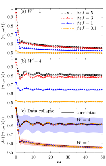
In this paper, we routinely choose $N=300$, which turns out to be sufficiently large to ensure reliable results. As an illustration, the standard deviation

$$\Delta\langle n_{l}(t)\rangle=\sqrt{\overline{\Big{[}\langle n_{l}(t)\rangle\Big{]}^{2}}-\Big{[}\overline{\langle n_{l}(t)\rangle}\Big{]}^{2}}$$ (15)

is later shown in Fig. 3 (c) for disorder strengths $W=1$ and $W=4$. Although one finds that $\Delta\langle n_{l}(t)\rangle$ becomes significantly larger for increasing $W$, the error of the average $\Delta\langle n_{l}(t)\rangle/\sqrt{N}$ remains well-controlled in all cases.

IV Results

After the introduction of the non-equilibrium setup and the class of initial states, we now turn to a discussion of the induced dynamics. First, we discuss in Sec. IV.1 the independence of these dynamics of the perturbation strength. Then, we discuss two important consequences and present specific numerical results, in the context of thermalization (Sec. IV.2) and transport (Sec. IV.3).

IV.1 Independence of the perturbation strength

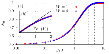
Let us start by presenting numerical results. As a first step, we study the expectation value $\langle n_{L/2}(t)\rangle$, i.e., we measure the occupation-number operator $n_{l}$ at the same lattice site $l=L/2$ which is used to prepare the initial state. Before discussing dynamics, it is instructive to study the dependence of the initial expectation value ${\cal N}_{0}=\langle n_{L/2}(0)\rangle$ on the strength of the perturbation. In Fig. 2, ${\cal N}_{0}$ is shown for a high temperature $\beta J=0.01$ up to a perturbation strength $\beta\varepsilon J\leq 10$. One observes that ${\cal N}_{0}$ increases linearly for small $\varepsilon$ [see Fig. 2 (b)] and eventually saturates for larger $\varepsilon$ to the maximum eigenvalue $n_{\text{max}}=1$. Furthermore, as expected for such high temperatures, ${\cal N}_{0}$ is independent of the Hamiltonian and therefore the curves for $W=1$ and $W=4$ in Fig. 2 are practically indistinguishable. The vertical dashed lines in Fig. 2 indicate those values of $\varepsilon$ which will be used in the following for the study of dynamics. Note that these values are chosen in such a way that we cover the whole range from states close to equilibrium up to states which are maximally perturbed.

Figure 2: (Color online) Initial expectation value ${\cal N}_{0}=\langle n_{L/2}(0)\rangle$ versus perturbation strength $\varepsilon$ for a high temperature $\beta J=0.01$. Panel (a): Semi-logarithmic ($x$ axis) plot. The vertical dashed lines indicate those values of $\varepsilon$ which are used to study dynamics, i.e., $\beta\varepsilon J=0.1,1,3,5$. Panel (b): Same data as in (a), but now in a linear plot. The linear prediction from Eq. (10) is shown. Note that for sufficiently small $\varepsilon$, the response is always small compared to the disorder potential $W$. The other parameters are $L=20$ and $\Delta=1.5$.

Let us now discuss dynamical expectation values. In Figs. 3 (a) and (b), $\langle n_{L/2}(t)\rangle$ is shown for a high temperature $\beta J=0.01$ and various perturbation strengths $\varepsilon$ for two different disorder values $W=1$ and $W=4$. Starting with the case $W=1$, we find a quick decay of $\langle n_{L/2}(t)\rangle$ at short time scales $tJ\lesssim 5$, followed by a significantly slower decay towards the long-time value $\langle n_{L/2}(t\to\infty)\rangle\sim n_{\text{eq}}=1/2$ (although this value is not yet reached at the maximum time shown here). On the other hand, for $W=4$, $\langle n_{L/2}(t)\rangle$ exhibits some oscillations which are absent in the case of $W=1$ (cf. Ref. Prelovsek2017 ), and more importantly, we clearly find a long-time value $\langle n_{L/2}(t\rightarrow\infty)\rangle\gg n_{\text{eq}}$. Since the initial values $\langle n_{L/2}(0)\rangle$ depend on the specific value of the perturbation $\varepsilon$ (cf. Fig. 2), all curves in Figs. 3 (a) and (b) naturally differ from each other. However, following the approach introduced in Ref. Richter2017 , a simple rescaling of the form

$$\mathcal{M}(\langle n_{l}(t)\rangle)=a\langle n_{l}(t)\rangle+b\ ,$$ (16)

with time-independent coefficients $a$ and $b$,

$$a=\frac{n_{\text{max}}-n_{\text{eq}}}{\langle n_{L/2}(0)\rangle-n_{\text{eq}}}\ ;\quad b=(1-a)n_{\text{eq}}\ ,$$ (17)

leads to a collapse of the data for different $\varepsilon$ onto a single curve, as shown in Fig. 3 (c). Thus, independent of the specific value of $\varepsilon$, i.e., independent of the initial state being close to or far away from equilibrium, the resulting time dependence is universal. Specifically, due to the projection property $n_{l}^{2}=n_{l}$, one can write Richter2017

$$\langle n_{l}(t)\rangle=\frac{n_{\text{eq}}+(e^{\beta\varepsilon}-1)\langle n_{l}(t)n_{L/2}\rangle_{\text{eq}}}{1+(e^{\beta\varepsilon}-1)n_{\text{eq}}}\ ,$$ (18)

i.e., our non-equilibrium dynamics at high temperatures is always given by a correlation function at equilibrium.

Thus, we end up with an intriguing situation: The class of initial states $\ket{\psi(0)}$, as introduced in Eq. (4), realizes a dynamics where the long-time limit $\langle n_{L/2}(t\rightarrow\infty)\rangle$ clearly depends (i) on the value of $\varepsilon$ and (ii) on the strength of the disorder $W$, in particular for $W>W_{\text{c}}$. On the other hand, the overall time dependence of $\langle n_{L/2}(t)\rangle$ is completely independent of $\varepsilon$. Remarkably, this result also holds true for rather strong disorder $W=4$, where the ETH is known to be violated. This fact also illustrates nicely that typicality of random states is unrelated to the validity of the ETH.

Figure 3: (Color online) Dynamical expectation value $\langle n_{L/2}(t)\rangle$ for a high temperature $\beta J=0.01$ and various perturbation strengths $\varepsilon$ up to times $tJ\leq 50$. Panels (a) and (b) show data for disorder strengths $W=1$ and $W=4$. Panel (c) shows a collapse of the data according to Eq. (16). The solid line indicates the (normalized) equilibrium correlation function $\langle n_{L/2}(t)n_{L/2}\rangle_{\text{eq}}$. The shaded area indicates the statistical fluctuations $\overline{\langle n_{l}(t)\rangle}\pm\Delta\langle n_{l}(t)\rangle$ [cf. Eq. (15)] due to the random potentials. Note that the error of the mean $\Delta\langle n_{l}(t)\rangle/\sqrt{N}$ is significantly smaller. The other parameters are $L=20$, $\Delta=1.5$, and $N=300$.

The above universality of the time dependence results since the occupation-number operators $n_{l}$ satisfy the projection property $n_{l}^{2}=n_{l}$. However, this particular property is clearly lost if one defines the local densities according to a larger unit cell. In fact, already if the unit cell contains two sites, then the corresponding local density $d_{l}=n_{2l-1}+n_{2l}$ ($1\leq l\leq L/2$) is not a projection operator any more. Thus, a physically important question is: Does a similar type of dynamical universality also emerge in this case? If not, the previous discussion would have been about a mathematical singularness and not about physical properties of the system.

To answer this question, one can use the fact that all $n_{l}$ mutually commute. As a consequence, the exponential $e^{\beta\varepsilon d_{l^{\prime}}}=e^{\beta\varepsilon n_{2l^{\prime}-1}}\,e^{\beta\varepsilon n_{2l^{\prime}}}$ ($l^{\prime}=L/4$) can be written as a product of two individual exponentials. Therefore, using the projection property $n_{l^{\prime}}^{2}=n_{l^{\prime}}$ again, we find

$$e^{\beta\varepsilon d_{l^{\prime}}}=\Big{[}1+(e^{\beta\varepsilon}-1)n_{2{l^{\prime}}-1}\Big{]}\Big{[}1+(e^{\beta\varepsilon}-1)n_{2{l^{\prime}}}\Big{]}\,,$$ (19)

which can be multiplied out and, using the abbreviation $g(\beta\varepsilon)=e^{\beta\varepsilon}-1$, rewritten as

$$e^{\beta\varepsilon d_{l^{\prime}}}=1+g(\beta\varepsilon)\,d_{l^{\prime}}+g(\beta\varepsilon)^{2}\,n_{2{l^{\prime}}-1}n_{2{l^{\prime}}}\,.$$ (20)

For the dynamical expectation value $\langle d_{l}(t)\rangle=\text{Tr}[\rho(t)d_{l}]$ with the initial density matrix $\rho=e^{\beta\varepsilon d_{l^{\prime}}}/\text{Tr}[e^{\beta\varepsilon d_{l^{\prime}}}]$, this relation then yields

$$\langle d_{l}(t)\rangle=\frac{1+g(\beta\varepsilon)\langle d_{l^{\prime}}d_{l}(t)\rangle_{\text{eq}}+g(\beta\varepsilon)^{2}C(t)}{1+g(\beta\varepsilon)+g(\beta\varepsilon)^{2}/4}\,,$$ (21)

where we have also used the high-temperature averages $\langle d_{l}\rangle_{\text{eq}}=1$ for any $l$ and $\langle n_{l}n_{l^{\prime}}\rangle_{\text{eq}}=1/4$ for $l\neq l^{\prime}$. Clearly, this equation is different from Eq. (18) due to the factor $g(\beta\varepsilon)^{2}$ but, most importantly, because of the correlation function $C(t)=\langle n_{2{l^{\prime}}-1}n_{2{l^{\prime}}}\,d_{l}(t)\rangle_{\text{eq}}$. Thus, in general, the time dependence cannot be expected to be independent of the perturbation $\varepsilon$.

However, if we assume that correlation functions for particles and holes behave the same,

$$C(t)\overset{!}{=}\langle[1-n_{2{l^{\prime}}-1}][1-n_{2{l^{\prime}}}][2-d_{l}(t)]\rangle_{\text{eq}}\,,$$ (22)

we get $C(t)=\langle d_{l^{\prime}}d_{l}(t)\rangle_{\text{eq}}/2-1/4$ and, as a consequence, the nominator of Eq. (21) becomes

$$1+g(\beta\varepsilon)\langle d_{l^{\prime}}d_{l}(t)\rangle_{\text{eq}}+g(\beta\varepsilon)^{2}[\langle d_{l^{\prime}}d_{l}(t)\rangle_{\text{eq}}/2-1/4]\,.$$ (23)

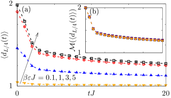
Therefore, in the case of a particle-hole symmetric system, the only time dependence is generated by the correlation function $\langle d_{l^{\prime}}d_{l}(t)\rangle_{\text{eq}}$, even in the case of a two-site unit cell for the definition of the local density. This prediction is also confirmed numerically in Fig. 4. We note that repeating the calculation for an ever larger unit cell yields higher powers in $g(\beta\varepsilon)$.

Figure 4: (Color online) Dynamical expectation value $\langle d_{L/4}(t)\rangle$ for a high temperature $\beta J=0.01$ and various perturbation strengths $\varepsilon$ up to times $tJ\leq 20$. Panel (b) shows a collapse of the data according to Eq. (16) with $d_{\text{eq}}=1$ and $d_{\text{max}}=2$. The other parameters are $L=20$, $\Delta=1.5$, and $W=1$.

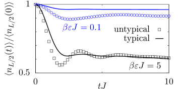
As already pointed out, Eq. (18) as well as Eq. (23) apply to the overwhelming majority of pure states drawn at random from a high-dimensional Hilbert space. But there should be counterexamples, of course. One of these counterexamples is a pure state $|\psi(0)\rangle$ which is still given by the definition in Eq. (4) but results from a specific reference state $|\varphi\rangle$ with all coefficients $c_{k}=\text{const.}$ being the same, to which we refer as an untypical state. Such a pure state $|\psi(0)\rangle$ is a valid member of the ensemble. However, the probability to draw this state at random is certainly tiny: ${\cal O}(2^{-L})$. For this untypical $|\psi(0)\rangle$, we show in Fig. 5 the time-dependent expectation value $\langle n_{L/2}(t)\rangle$ for different values of the perturbation $\varepsilon$ and a single set of other model parameters. Compared to Fig. 3, the time dependence is apparently different, and it does change with $\varepsilon$ as well.

Figure 5: (Color online) Comparison between a typical and an untypical state. The other parameters are $L=20$, $\Delta=1.5$, $W=1$, and $\beta J=0.01$.

IV.2 Eigenstate thermalization

Let us start with a discussion of the validity of the ETH. To study this validity for the Hamiltonian $\mathcal{H}$ in Eq. (II) and the occupation-number operator $n_{l}$, one can introduce the following two quantities Steinigeweg2014 :

$$\bar{n}=\sum_{i=1}^{2^{L}}p_{i}\bra{i}n_{l}\ket{i}\ ,\quad\Sigma^{2}=\sum_{i=1}^{2^{L}}p_{i}\bra{i}n_{l}\ket{i}^{2}-\bar{n}^{2}\ ,$$ (24)

with $\mathcal{H}\ket{i}=E_{i}\ket{i}$ as well as $p_{i}\propto e^{-(E_{i}-E)^{2}/2(\delta E)^{2}}$ and $\sum_{i}p_{i}=1$. Thus, $\bar{n}=\bar{n}(E,\delta E)$ is a weighted average of the diagonal matrix elements $n_{ii}=\bra{i}n_{l}\ket{i}$ in the eigenbasis of $\mathcal{H}$, and most sensitive to a (microcanonical) energy region of width $\delta E$ around $E$. Likewise, $\Sigma^{2}=\Sigma^{2}(E,\delta E)$ is a weighted variance of the $n_{ii}$ in this energy region. Moreover, since these quantities should be practically independent of the specific lattice site (if one averages over disorder), we just calculate them for a single $l\in[1,L]$. If the ETH applies, the diagonal matrix elements $n_{ii}$ should be a smooth function of energy in the thermodynamic limit. Consequently, $\Sigma^{2}$ should become small in this case Beugeling2014 ; Steinigeweg2013 . While it is certainly possible to obtain $\bar{n}$ and $\Sigma^{2}$ by exact diagonalization of small systems, we here also rely on a useful typicality-based approach Steinigeweg2014 to calculate these quantities for larger systems. Details on this approach are given in Appendix A.

In Figs. 6 (a) and (c), $\bar{n}$ as well as $\bar{n}\pm\Sigma$ are shown in the energy range $E/J=[-3,3]$ (roughly in the center of the spectrum), for the two disorder strengths $W=1$ and $W=4$, respectively. In both cases, we choose an energy resolution $\delta E/J=0.5$. Moreover, we compare data for $L=12$ (exact diagonalization) and $L=20$ (typicality-based approach). Starting with the case $W=1$, we find that $\Sigma$ (i) becomes slightly larger for increasing $E$ (cf. Ref. Beugeling2014 ) and (ii) visibly decreases with increasing system size $L$. Although we do not perform a concrete finite-size scaling here (see e.g. Ref. Beugeling2014 for the disorder-free case $W=0$), Fig. 6 (a) is consistent with a vanishing $\Sigma$ in the thermodynamic limit, i.e., the ETH is fulfilled for the small disorder $W=1$. On the contrary, for $W=4$, one observes that $\Sigma$ is not a function of $E$ and, even more importantly, it does practically not scale with $L$ at all. Thus, for $L\to\infty$, $\Sigma$ will be nonzero and the ETH is violated for the strong disorder $W=4$.

The apparent differences between the two cases $W=1$ and $W=4$ are also clearly visible when studying the cloud of diagonal matrix elements directly. In Figs. 6 (b) and (d), the matrix elements $n_{ii}$ are shown versus the corresponding eigenenergies $E_{i}$, whereby we focus on a single subspace with $L/4$ fermions ($L=20$) and consider only a single realization of disorder ($N=1$). While in the case of $W=1$ the $n_{ii}$ are aligned relatively close to each other, they appear randomly distributed for $W=4$ with enhanced probability at the extrema $n_{ii}=0$, $1$ (see Ref. Roy2018 for similar results).

Figure 6: (Color online) Panels (a) and (c): Weighted average $\bar{n}\pm\Sigma$ in the energy range $-3\leq E/J\leq 3$ for $W=1$ and $W=4$, respectively. Filled symbols are exact-diagonalization results for $L=12$, open symbols are obtained by the typicality-based approach for $L=20$. The microcanonical window around $E/J\approx 0$ corresponds to high temperatures $\beta J\approx 0$. Panels (b) and (d): Distribution of diagonal matrix elements $n_{ii}$ versus eigenenergy $E_{i}$ in the subspace with $L/4$ fermions ($L=20$). The other parameters are $\delta E/J=0.5$ and $\Delta=1.5$.

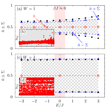
Let us now establish a relation between the quantities $\bar{n}$ and $\Sigma$ and the non-equilibrium dynamics $\langle n_{l}(t)\rangle$ discussed before. In view of Eq. (18), we find that the long-time value of $\langle n_{l}(t)\rangle$ follows as (see also Appendix A)

$$\langle n_{L/2}(t\to\infty)\rangle=c_{1}+c_{2}(\bar{n}^{2}+\Sigma^{2})\ ,$$ (25)

with the two $\beta\epsilon$ dependent coefficients

$$c_{1}=\frac{n_{\text{eq}}}{1+(e^{\beta\varepsilon}-1)n_{\text{eq}}}\ ;\ c_{2}=\frac{e^{\beta\varepsilon}-1}{1+(e^{\beta\varepsilon}-1)n_{\text{eq}}}\ .$$ (26)

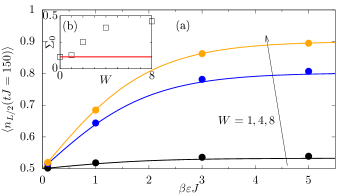
One readily sees that for $\Sigma=0$ (and $\bar{n}=n_{\text{eq}}$), Eq. (25) reduces to $\langle n_{L/2}(t\to\infty)\rangle=n_{\text{eq}}$, independent of $\beta\epsilon$. Thus, if $\Sigma=0$, $\langle n_{l}(t)\rangle$ relaxes towards the equilibrium value $n_{\text{eq}}$, irrespective of $\beta\epsilon$. In contrast, if $\Sigma>0$, $\langle n_{l}(t)\rangle$ does not reach its equilibrium value at long times and, in particular, this long-time value is directly given by the width of the distribution of the diagonal matrix elements. Note that in any finite system one expects

$$\Sigma\geq\Sigma_{\text{min}}=\frac{1}{\sqrt{4L}}\ ,$$ (27)

which is a consequence of Eq. (25) and $\langle n_{L/2}(t\to\infty)\rangle\geq({\cal N}_{0}-n_{\text{eq}})/L+n_{\text{eq}}$, i.e., the initial $\delta$ peak is eventually distributed over a finite number of lattice sites only.

It is important to stress that the quantities $\bar{n}(E)$ and $\Sigma(E)$ on the r.h.s. of Eq. (25) have to be chosen from a microcanonical energy window $[E-\delta E,E+\delta E]$ corresponding to high temperatures $\beta J\approx 0$, in the sense of the equivalence of ensembles. While this procedure might not be justified a priori in a disordered system, we depict in Fig. 7 (a), the long-time value of $\langle n_{L/2}(t)\rangle$, extracted at time $tJ=150$ and for the parameters in Fig. 3 (see also Appendix B). Moreover, we compare these data with the prediction in Eq. (25), where $\Sigma_{0}=\Sigma(E/J=0)$ should correspond to $\beta J\approx 0$. Generally, one observes a convincing agreement of the data for all values of $W$ and $\beta\epsilon$ shown here. The residual deviations are presumably not only caused by statistical fluctuations due to the random potentials, but also by the finite time $tJ=150$ considered. (Note that the symbols lie above the solid lines.) Overall, however, Fig. 7 (a) confirms Eq. (25), which implies that the validity of the ETH is a necessary condition for the thermalization of our class of initial states.

Figure 7: (Color online) Panel (a): Numerical illustration of the validity of Eq. (25). The data points are extracted from the non-equilibrium dynamics $\langle n_{L/2}/(t)\rangle$ at time $tJ=150$, while the solid lines are calculated according to Eq. (25) with $\Sigma_{0}=\Sigma(E/J=0)$. In addition to the cases $W=1$ and $W=4$, we also show data for the case $W=8$ (see Appendix B). Panel (b): $\Sigma_{0}$ versus disorder $W$. For comparison, the lower bound $\Sigma_{\text{min}}=1/\sqrt{4L}$ is indicated, which follows from Eq. (25) and $\langle n_{L/2}(t\to\infty)\rangle\geq({\cal N}_{0}-n_{\text{eq}})/L+n_{\text{eq}}$ in systems of finite size (horizontal line). In all cases, we have $L=20$ and $\Delta=1.5$.

IV.3 Broadening of non-equilibrium profiles

So far, we have only considered the single expectation value $\langle n_{L/2}(t)\rangle$. Now, we intend to discuss the dynamics of $\langle n_{l}(t)\rangle$ for all $1\leq l\leq L$. First, let us reiterate that the states $\ket{\psi(0)}$ realize an initial density profile with a $\delta$ peak on top of a homogeneous many-particle background, cf. Eq. (13). This $\delta$ peak will gradually broaden over time according to the Schrödinger equation, and we aim at classifying the particular type of broadening.

To begin with, the real-time and real-space dynamics of $\langle n_{l}(t)\rangle$ can be said to be diffusive, if it fulfills the lattice diffusion equation Michel2005 ; Steinigeweg2007

$$\frac{\text{d}}{\text{d}t}\langle n_{l}(t)\rangle=D[\langle n_{l-1}(t)\rangle-2\langle n_{l}(t)\rangle+\langle n_{l+1}(t)\rangle]\ ,$$ (28)

where $D$ is a time-independent diffusion constant. For our initial $\delta$ profile, a specific solution of Eq. (28) is given in terms of a Bessel function Richter2018 , which (for sufficiently large $L$ and long $t$) can be very well approximated by the Gaussian function

$$\langle n_{l}(t)\rangle-n_{\text{eq}}\propto\exp\left[-\frac{(l-L/2)^{2}}{2\sigma^{2}(t)}\right]\ ,$$ (29)

with the spatial variance $\sigma^{2}(t)=2Dt$. Thus, in case of diffusive transport, $\langle n_{l}(t)\rangle$ must be a Gaussian profile of width $\sigma(t)\propto\sqrt{t}$. For any type of transport, the spatial variance $\sigma^{2}(t)$ can be also obtained from $\langle n_{l}(t)\rangle$ according to Richter2018 ; Karrasch2014 ; Steinigeweg2017

$$\sigma^{2}(t)=\sum_{l=1}^{L}l^{2}\,\delta n_{l}(t)-\left(\sum_{l=1}^{L}l\ \delta n_{l}(t)\right)^{2}\ ,$$ (30)

where $\delta n_{l}(t)=(\langle n_{l}(t)\rangle-n_{\text{eq}})/({\cal N}_{0}-n_{\text{eq}})$ is introduced such that $\sum_{l}\delta n_{l}(t)=1$. For our initial states and any perturbation $\varepsilon$ (in the high-temperature limit $\beta J\approx 0$), it follows that the time-derivative of the spatial variance $\sigma^{2}(t)$ is given by Steinigeweg2009 ; Steinigeweg2009_2 ; Karrasch2017 ; Yan2015 ,

$$\frac{\text{d}}{\text{d}t}\sigma^{2}(t)=2D(t)\ ,$$ (31)

where $D(t)$ plays the role of a time-dependent diffusion coefficient and is connected to the current autocorrelation function at equilibrium via the generalized Einstein relation

$$D(t)=\frac{1}{\chi}\int_{0}^{t}\langle j(t^{\prime})j\rangle_{\text{eq}}\ \text{d}t^{\prime}\ ,$$ (32)

with the static susceptibility $\chi=1/4$ for $\beta\rightarrow 0$.

Very often, it is instructive to study density dynamics in momentum space as well Steinigeweg2011 ; Bera2017 . A Fourier transform of the lattice diffusion equation in Eq. (28) yields

$$\frac{\text{d}}{\text{dt}}\langle n_{q}(t)\rangle=-2(1-\cos q)D_{q}(t)\langle n_{q}(t)\rangle\ ,$$ (33)

where one additionally allows for a time- and momentum-dependent diffusion coefficient $D_{q}(t)$ Steinigeweg2011 . As usual, the lattice momentum $q$ takes on the discrete values values $q=2\pi k/L$ with $k=0,1,\dots,L-1$. In the limit of small $q$, and for our non-equilibrium setup, this $D_{q}(t)$ coincides with the $D(t)$ in Eq. (32).

The behavior of $D_{q}(t)$ can be manifold: On the one hand, in the short-time limit, $D_{q}(t)$ is independent of $q$ and scales ballistically as $D_{q}(t)\propto t$. On the other hand, outside this trivial short-time limit, $D_{q}(t)$ can in principle have any dependence on $q$ and $t$. Nevertheless, diffusion clearly requires $D_{q}(t)=\text{const.}$ in a hydrodynamic regime of sufficiently small $q$ and long $t$. In contrast, different types of transport like subdiffusion (superdiffusion) can be defined as power-law scaling of the form $D_{q}(t)\propto t^{\alpha}$ with $\alpha<0$ ($\alpha>0$). Note that $D_{q}(t)$ does not distinguish between coexisting transport channels Sirker2009 .

Figure 8: (Color online) Panels (a) and (c): Density profile $\langle n_{l}(t)\rangle$ for disorder strengths $W=1$ and $W=4$, respectively. The initial state is prepared according to Eq. (4) with $\beta J=0.01$ and $\beta\varepsilon J=3$. Panels (b) and (d): Corresponding width $\sigma(t)$ for various $\beta\varepsilon$, obtained from Eq. (30). For comparison, we also depict $\sigma(t)$ from the current autocorrelation function, calculated according to Eq. (31). The dashed vertical line is a guide to the eye. The other parameters are $L=20$ and $\Delta=1.5$.

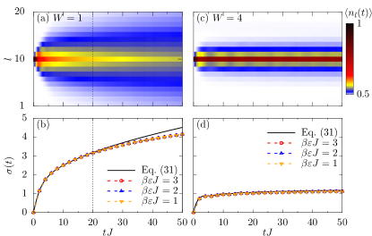
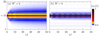
Let us now present our numerical results. In Fig. 8 (a), we depict the time evolution of the non-equilibrium density profile $\langle n_{l}(t)\rangle$ for a moderate disorder $W=1$ up to times $tJ\leq 50$. On the one hand, we can clearly observe the initial $\delta$ profile at $t=0$. On the other hand, this profile broadens relatively quickly and reaches the boundaries of the system at $tJ\approx 20$ (as indicated by the dashed vertical line). In Fig. 8 (b), the corresponding width $\sigma(t)$ of the density profile is shown. In agreement with our earlier discussion of the universal dynamics in Sec. IV.1, we find that also $\sigma(t)$ is independent of the perturbation $\varepsilon$. Furthermore, according to our discussion in the context of Eqs. (30) and (31), we compare the profile width to the width obtained from the current autocorrelation function. While for short times $tJ\lesssim 20$, we find a good agreement between both widths, one clearly observes deviations at longer times. These deviations can be explained by the fact that a calculation of $\sigma^{2}(t)$ according to Eq. (31) is not justified anymore if the width of the density profile becomes comparable to the size of the system Steinigeweg2009 . It also important to note that a visualization of the data as done here nicely illustrates the time scales where finite-size effects due to boundary effects become non-negligible.

In Figs. 8 (c) and (d) we show results for the larger disorder $W=4$. In contrast to the previous case of $W=1$, the initial $\delta$ peak broadens significantly slower and, even at times $tJ=50$, the boundary is not reached yet. This fact is also reflected by the width $\sigma(t)$ which, after an initial increase below $tJ\lesssim 5$, saturates to a constant plateau. Moreover, in this case, the agreement between calculations of $\sigma(t)$ via Eq. (30) and Eq. (31) is excellent for all times depicted.

Figure 9: (Color online) Time dependence of the generalized diffusion coefficient $D_{q}(t)$ for wave vectors $k=0$ [Eq. (32)] and $k=1,2$ [Eq. (33)], for three disorders $W=0$, $0.5$ and $1$, respectively. For $k=0$, data are always shown for two system sizes: (a) $L=20$ and $L=34$; (b) and (c) $L=20$ and $L=26$. For $k=1,2$, we have $L=20$ in all cases. Other parameters: $\Delta=1.5$.

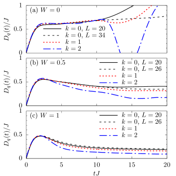
We now turn to studying the broadening of the $\delta$ peak in more detail. Specifically, we restrict ourselves to the parameter regime of small disorder $W\leq 1$ Luitz2017 ; Agarwal2015 ; Gopalakrishnan2015 ; BarLev2015 ; Luitz2016 ; Khait2016 , where sample-to-sample fluctuations are still small, cf. Fig. 3 (c). In Fig. 9, the diffusion coefficient $D_{q}(t)$ is depicted for momenta $q/(2\pi/L)=0$, $1$, $2$, times $tJ\leq 20$, and disorder $W=0$, $0.5$, $1$, i.e., including the disorder-free case $W=0$. For this clean case, we find that $D_{q}(t)$ is approximately constant for times $2\lesssim tJ\lesssim 10$. Furthermore, at these times, we find that $D_{q}(t)$ coincides for all three momenta $q$ depicted Steinigeweg2011 ; Richter2018 . Visible differences for longer times are a consequence of finite-size effects, as evident when comparing the two $q=0$ curves for $L=20$ and $L=34$ Steinigeweg2014_2 . Hence, for $\Delta=1.5$, we clearly find diffusion in the absence of disorder Prelovsek2004 ; Znidaric2011 ; Steinigeweg2011 ; Karrasch2014 ; Steinigeweg2017 ; Ljubotina2017 . In fact, to have this well-behaving point of reference, we have chosen $\Delta=1.5$ throughout our paper, in contrast to the vast majority of works on disordered systems, which study the isotropic point $\Delta=1$.

When switching on small disorder $W>0$, one clearly observes two changes. First, quite counterintuitively, the number of coinciding $q$ is reduced. However, at least the two smallest momenta $q/(2\pi/L)=0$ and $1$ behave still the same way. Second, after the initial increase of $D_{q}(t)$, it decreases again. Nevertheless, this decrease then turns into a minor time dependence of $D_{q}(t)$. Hence, at times $10\lesssim tJ\lesssim 20$, no big error results when approximating $D_{q}(t)$ by a constant. Certainly, one might be tempted to consider even longer times. But finite-size effects appear at such times, as evident when comparing the two $q=0$ curves for $L=20$ and $L=26$ ($\ll 34$). And surely, one might be tempted to analyze the minor time dependence in more detail. But such an endeavor is meaningless, as the spanned scale at the $y$ axis is much smaller than one order of magnitude. Consequently, we conclude that our data for small disorder $W=0.5$ and $1$ are still consistent with diffusion, while it cannot rule out subdiffusion.

Figure 10: (Color online) Density profile $\langle n_{l}(t)\rangle$ for the three disorder strengths (a) $W=0$, (c) $W=0.5$, (e) $W=1$ and a short time $tJ=5$, in a semi-logarithmic plot ($y$ axis). For each $W$, a longer time is shown in (b), (d), (f), where boundary effects are still negligibly small. In all (a)-(f), Gaussian fits are indicated for comparison. In (f), an exponential fit to the outer tails is depicted. Other parameters: $\Delta=1.5$.

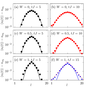
To shed further light onto the differences between the clean case $W=0$ and the disordered cases $W>0$, we summarize in Fig. 10 the site dependence of the density profile $\langle n_{l}(t)\rangle$ for $W=0$ (top row), $W=0.5$ (middle row), and $W=1$ (bottom row). Furthermore, we do so for a short time $tJ=5$ (left column) and a longer time (right column), where boundary effects are still negligibly small. For no or weak disorder, $W=0$ and $W=0.5$, and all times depicted, one can clearly see that the density profile $\langle n_{l}(t)\rangle$ is very well described by Gaussian fits over roughly two orders of magnitude. In agreement with our earlier conclusions, this pronounced Gaussian form of the density profile provides another strong evidence for the existence of diffusion (see also Ref. Steinigeweg2017 for $W=0$).

Figure 11: (Color online) Same data as in Fig. 10 but now shown for $W=2$.

For stronger disorder $W=1$ and a short time $tJ=5$, the density profile can be still described in terms of a Gaussian. It is apparent, however, that the agreement is much less convincing. In contrast, for a longer time $tJ=15$, a Gaussian description clearly fails and is, in particular, not able to capture the outer tails of $\langle n_{l}(t)\rangle$ correctly. Instead, these tails appear to be exponential, and the overall density profile has a triangular shape in the semi-logarithmic plot used. This shape is a signature of non-diffusive dynamics and might be thus consistent with subdiffusion in this parameter regime Znidaric2016 . Despite of larger sample-to-sample fluctuations, we find similar results for $W=2$, see Fig. 11.

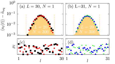
Remarkably, since sample-to-sample fluctuations are small for a small amount of disorder, the density profiles $\langle n_{l}(t)\rangle$ can be accurately obtained already from a single realization of the random potential. To demonstrate this fact, we repeat the calculation for $W=0.5$ and $tJ=10$ in Fig. 10 (d), but without any averaging over disorder configurations. Moreover, we do so for two substantially larger system sizes $L=30$ and $31$, where the Hilbert space is huge. As summarized in Fig. 12, the corresponding results agree very well with the averaged $N=20$ results, even in the semi-logarithmic plot used again. This agreement also demonstrates that finite-size effects are small on this time scale. Note that the calculations for $L\geq 30$ have been carried out only for the largest particle subsector, in contrast to all other calculations in this paper. Note further that $\tilde{n}_{\text{eq}}=\langle n_{l\neq L/2}(0)\rangle$ is not strictly identical to $n_{\text{eq}}=1/2$ but reads

$$\tilde{n}_{\text{eq}}={{L-2}\choose{L/2-2}}/{{L-1}\choose{L/2-1}}\$$ (34)

in the half-filling sector ($\tilde{n}_{\text{eq}}\approx 0.483$ for $L=30$).

V Conclusion

In summary, we have studied the real-time dynamics of local occupation numbers in a one-dimensional model of spinless fermions with a random on-site potential for a certain class of initial states. These initial states are thermal (mixed or pure) states of the model in the presence of an additional static force, but become non-equilibrium states after a sudden removal of this static force. For this class and high temperatures, we have shown that the induced dynamics is given by a single correlation function at equilibrium, independent of the initial expectation values being prepared close to equilibrium (by a weak static force) or far away from equilibrium (by a strong static force). Remarkably, this type of universality holds true in both, the ergodic phase and the many-body localized regime. Moreover, it does not depend on the specific choice of a unit cell for the local density.

We have particularly discussed two important consequences. First, the long-time expectation value of the local density is uniquely determined by the fluctuations of its diagonal matrix elements in the energy eigenbasis. Thus, the validity of the eigenstate thermalization hypothesis is not only a sufficient but also a necessary condition for thermalization. Second, the real-time broadening of density profiles is always given by the current autocorrelation function at equilibrium via a generalized Einstein relation. In the context of transport, we have discussed the influence of disorder for large particle-particle interactions, where normal diffusion is known to occur in the disorder-free case. Our results suggest that normal diffusion is stable against weak disorder, while they are consistent with anomalous diffusion for non-weak disorder.

Promising future research directions include the generalization to different non-equilibrium scenarios as well as the study of lower temperatures.

Figure 12: (Color online) Density profile $\langle n_{l}(t)\rangle$ for $W=0.5$ and single realizations of the random on-site potential: Two different realizations for (a) $L=30$ and (b) $L=31$ sites. These unaveraged data (symbols) are additionally compared to averaged $N=20$ data (shaded area) from Fig. 10 (d) with $tJ=10$. (c), (d) Corresponding realizations of the random on-site potential. Note that we restrict ourselves to the largest subsector of ($L=30$) or around $(L=31)$ half filling.

Acknowledgements

This work has been funded by the Deutsche Forschungsgemeinschaft (DFG) - STE 2243/3-1. We sincerely thank the members of the DFG Research Unit FOR 2692 for fruitful discussions. J.H. has been supported by the US Department of Energy (DOE), Office of Science, Basic Energy Sciences (BES), Materials Sciences and Engineering Division.

Appendix A ETH and typicality

For completeness, we describe in this section how to calculate the ETH quantities $\bar{n}$ and $\Sigma^{2}$ in Eq. (24) by means of a typicality-based approach. While we closely follow the derivations presented in Ref. Steinigeweg2014 , we also show that Eq. (25) follows from these derivations.

First, we introduce the pure state $\ket{\psi_{E}}$,

$$\ket{\psi_{E}}=C_{E}\ket{\varphi}\quad;\quad C_{E}=e^{-\frac{(\mathcal{H}-E)^{2}}{4(\delta E)^{2}}}\ ,$$ (35)

where $\ket{\varphi}$ is again a random state drawn according to the unitary invariant Haar measure (cf. Eq. (4) and below) and the operator $C_{E}$ is an energy filter of Gaussian type Steinigeweg2014 ; Garnerone2013 , $C_{E}^{2}=\exp[-(\mathcal{H}-E)^{2}/2(\delta E)^{2}]$. Exploiting the concept of typicality, the quantity $\bar{n}(E)$ can then be obtained according to

$$\bar{n}(E)\approx\frac{\bra{\psi_{E}}n_{l}\ket{\psi_{E}}}{\braket{\psi_{E}}{\psi_{E}}}\ ,$$ (36)

where the statistical error due to $\ket{\varphi}$ and the dependence on $\delta E$ have been dropped for clarity. Next, in order to calculate $\Sigma(E)$, we define

$$\gamma_{E}(t) =\frac{\bra{\psi_{E}}n_{l}(t)n_{l}\ket{\psi_{E}}}{\braket{\psi_{E}}{\psi_{E}}}$$ (37)

$$=\frac{\bra{\psi_{E}(t)}n_{l}\ket{\tilde{\psi}_{E}(t)}}{\braket{\psi_{E}}{\psi_{E}}}\ ,$$ (38)

where $\ket{\tilde{\psi}_{E}}=n_{l}\ket{\psi_{E}}$ and $\ket{\psi_{E}(t)}=e^{-i\mathcal{H}t}\ket{\psi_{E}}$. Now, we require that $\gamma_{E}(t)$ relaxes with time to some value and then stays approximately constant. Note that, from a numerical point of view, this relaxation should be also sufficiently fast, to make our approach efficient. Given this requirement, we find that the long-time average of $\gamma_{E}(t)$ is given by Steinigeweg2014

$$\bar{\gamma}_{E}=\frac{1}{t_{2}-t_{1}}\int_{t_{1}}^{t_{2}}\text{d}t\ \gamma_{E}(t)\approx\bar{n}(E)^{2}+\Sigma(E)^{2}\ .$$ (39)

Thus, it is possible to obtain $\Sigma(E)$ according to

$$\Sigma(E)=\sqrt{\bar{\gamma}_{E}-\bar{n}(E)^{2}}\ ,$$ (40)

with $\bar{n}(E)$ as given in Eq. (36).

Note that Eq. (39) implies the validity of Eq. (25) in the main text because of two reasons: (i) $\gamma(t)$ is nothing else than the equilibrium correlation function $\langle n_{l}(t)n_{l}\rangle_{\text{eq}}$ within the approximate microcanonical energy window $[E-\delta E,E+\delta E]$. (ii) In the context of Eq. (18), we have discussed that $\langle n_{l}(t)\rangle\propto\langle n_{l}(t)n_{l}\rangle_{\text{eq}}$ within the canonical ensemble at high temperatures $\beta\approx 0$. Thus, in the sense of the equivalence of ensembles, there is a direct relation between the long-time values of $\gamma(t)$ and $\langle n_{l}(t)\rangle$, if the microcanonical energy $E$ is chosen is such a way that it corresponds to the canonical temperature $\beta\approx 0$.

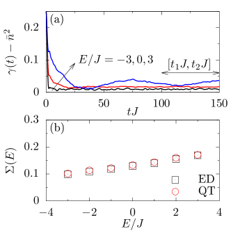
To illustrate the accuracy of this pure-state approach, we compare in Fig. 13 (b) the width $\Sigma(E)$, as obtained from the exact definition in Eq. (24), with the width $\Sigma(E)$, as obtained from Eqs. (38) – (40) within the time interval $[t_{1}J,t_{2}J]=[100,150]$, cf. Fig. 13 (a). We find a very good agreement between both approaches, already for the small system with $L=14$ sites. Note that, while we average here over $N=300$ realizations of the pure state $\ket{\varphi}$ to reduce statistical fluctuations, this averaging becomes less important for increasing system size.

Figure 13: (Color online) Panel (a): Quantity $\gamma(t)-\bar{n}^{2}$ according to Eqs. (36) and (38) for $L=14$ sites, averaged over $N=300$ random realizations of the pure state $\ket{\varphi}$. Data are shown for energies $E/J=-3,0,3$. Panel (b): Comparison of the width $\Sigma(E)$, as obtained from the exact definition in Eq. (24), with the width $\Sigma(E)$, as obtained from Eqs. (38) – (40) with the time interval $[t_{1}J,t_{2}J]=[100,150]$. The other parameters are $\Delta=1.5$ and $W=0$.

Appendix B Longer times and other values of disorder

In the main text, we have mainly focused on the two disorder strengths $W=1$ and $4$ and considered times up to $tJ\leq 50$. For completeness, let us here also show data for $W=2$ and $8$ as well as longer times. Note that these data has been already used in the context of Fig. 7.

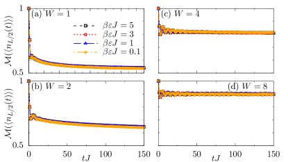
For the dynamical expectation value $\langle n_{L/2}(t)\rangle$ at the single site site $l=L/2$, we depict in Fig. 14 the data collapse ${\cal M}(\langle n_{L/2}(t)\rangle)$ for disorder strengths $W=1$, $2$, $4$, and $8$ up to long times $tJ\leq 150$. For the intermediate disorder $W=2$, one finds that even at these long times, $\langle n_{L/2}(t)\rangle$ has not yet reached its final value.

Figure 14: (Color online) Data collapse ${\cal M}(\langle n_{L/2}(t)\rangle)$, cf. Eq. (16), for perturbations $\beta\varepsilon J=0.1,1,3,5$ and disorder strengths $W=1,2,4,8$ up to long times $tJ\leq 150$. The other parameters are $L=20$ and $\Delta=1.5$.

Additionally, we show in Fig. 15 the time evolution of the full density profile $\langle n_{l}(t)\rangle$, $0\leq l\leq L$, for the two disorder strengths $W=2$ and $8$, complementary to the data already presented in Fig. 8. While the $\delta$ peak broadens for $W=2$, the dynamics are essentially frozen for $W=8$.

Appendix C Calculation of correlation functions

The numerical calculation of equilibrium correlation functions such as $\langle n_{l}(t)n_{l}\rangle_{\text{eq}}$ or $\langle j(t)j\rangle_{\text{eq}}$ is an important aspect of our paper. Thus, let us briefly describe how these dynamical quantities can be obtained from both, exact diagonalization and a typicality-based pure-state approach. In this context, we also comment on the class of non-equilibrium pure states $\ket{\psi(0)}$ in Eq. (4) in more detail.

For simplicity, we focus on the equilibrium correlation function $\langle n_{l}(t)n_{l}\rangle_{\text{eq}}$. For the use of exact diagonalization, this correlation function is conveniently written in terms of the eigenstates $\ket{a}$ and the corresponding eigenvalues $E_{a}$ of the Hamiltonian $\mathcal{H}$,

$$\langle n_{l}(t)n_{l}\rangle_{\text{eq}} =\frac{\text{Tr}[e^{-\beta\mathcal{H}}\,n_{l}(t)n_{l}]}{\mathcal{Z}_{\text{eq}}}$$ (41)

$$=\sum_{a,b=1}^{2^{L}}\frac{e^{-\beta E_{a}}}{\mathcal{Z}_{\text{eq}}}\,|\!\bra{a}n_{l}\ket{b}\!|^{2}\,e^{i(E_{a}-E_{b})t}\ ,$$ (42)

with $\mathcal{Z}_{\text{eq}}=\sum_{a}e^{-\beta E_{a}}$. Because of the random potentials, exact diagonalization becomes relatively costly for systems with $L\sim 14$ sites already since (i) translational invariance is broken and (ii) also an averaging over a sufficiently large number of instances of these random potentials is required.

Using the concept of quantum typicality, on the other hand, the trace in Eq. (41) can be replaced by a scalar product with a single pure state $\ket{\varphi}$, which is drawn at random according to the Haar measure, i.e., according to Eq. (5) with Gaussian distributed coefficients $c_{k}$. Thus, by introducing the two auxiliary pure states Elsayed2013 ; Steinigeweg2014_2 ; iitaka2003

$$\ket{\phi(t,\beta)} =e^{-i\mathcal{H}t}\,n_{l}\,e^{-\beta\mathcal{H}/2}\,\ket{\varphi}\ ,$$ (43)

$$\ket{\varphi(t,\beta)} =e^{-i\mathcal{H}t}\,e^{-\beta\mathcal{H}/2}\,\ket{\varphi}\ ,$$ (44)

we can rewrite the correlation function $\langle n_{l}(t)n_{l}\rangle_{\text{eq}}$ in the form

$$\langle n_{l}(t)n_{l}\rangle_{\text{eq}}=\frac{\bra{\varphi(t,\beta)}n_{l}\ket{\phi(t,\beta)}}{\braket{\varphi(0,\beta)}{\varphi(0,\beta)}}+f(\ket{\varphi})\ ,$$ (45)

where the statistical error $f(\ket{\varphi})$ decreases exponentially fast with increasing the Hilbert-space dimension.

The numerical evaluation of Eq. (45) can be done by the forward propagation (in real and imaginary time) of the two pure states $\ket{\varphi(t,\beta)}$ and $\ket{\phi(t,\beta)}$. As mentioned in the main body of the text, the involved operators $n_{l}$ and $\mathcal{H}$ exhibit a sparse-matrix representation such that these propagations can be implemented memory efficient, which particularly allows for a treatment of significantly larger systems compared to exact diagonalization. Note that Eq. (45), as well as Eq. (42), can be used for the current autocorrelation function $\langle j(t)j\rangle_{\text{eq}}$ as well, simply by replacing $n_{l}$ by $j$.

Eventually, let us comment on the non-equilibrium pure states $\ket{\psi(t)}$ and its expectation value $\langle n_{l}(t)\rangle$, as discussed in the main part of this paper. In the limit of small $\beta$, we have shown that (i) the non-equilibrium dynamics is independent of the perturbation $\varepsilon$ and that (ii) these dynamics are also identical to the equilibrium correlation function. Compared to the above typicality approach based on Eq. (45), one needs to propagate one pure state in (real and imaginary time) only, which is certainly a numerical advancement. It should be noted, however, that the properties (i) and (ii) are not expected to hold for lower temperatures, at least in general.

Figure 15: (Color online) Density profile $\langle n_{l}(t)\rangle$ for disorder strengths $W=2$ and $W=8$, respectively. The initial state is prepared according to Eq. (4) with the parameters $\beta J=0.01$ and $\varepsilon\beta J=3$. The other parameters are $L=20$ and $\Delta=1.5$.

References

- (1) A. Eckardt, C. Weiss, and M. Holthaus, Superfluid-insulator transition in a periodically driven optical lattice, Phys. Rev. Lett. 95, 260404 (2005).
- (2) A. Lazarides, A. Das, and R. Moessner, Periodic thermodynamics of isolated quantum systems, Phys. Rev. Lett. 112, 150401 (2014).
- (3) C. Mejía-Monasterio, T. Prosen, and G. Casati, Fourier’s law in a quantum spin chain and the onset of quantum chaos, EPL (Europhys. Lett.) 72, 520 (2005).
- (4) M. Michel, O. Hess, H. Wichterich, and J. Gemmer, Transport in open spin chains: A Monte Carlo wave-function approach, Phys. Rev. B 77, 104303 (2008).
- (5) M. Žnidarič, Spin transport in a one-dimensional anisotropic Heisenberg model, Phys. Rev. Lett. 106, 220601 (2011).
- (6) F. H. L. Essler, S. Kehrein, S. R. Manmana, and N. J. Robinson, Quench dynamics in a model with tuneable integrability breaking, Phys. Rev. B 89, 165104 (2014).
- (7) C. Karrasch, J. E. Moore, and F. Heidrich-Meisner, Real-time and real-space spin and energy dynamics in one-dimensional spin- systems induced by local quantum quenches at finite temperatures, Phys. Rev. B 89, 075139 (2014).
- (8) F. H. L. Essler and M. Fagotti, Quench dynamics and relaxation in isolated integrable quantum spin chains, J. Stat. Mech. 2016, 064002 (2016).
- (9) P. Reimann, Typical fast thermalization processes in closed many-body systems, Nat. Commun. 7, 10821 (2016).
- (10) J. Richter, F. Jin, H. De Raedt, K. Michielsen, J. Gemmer, and R. Steinigeweg, Real-time dynamics of typical and untypical states in nonintegrable systems, Phys. Rev. B 97, 174430 (2018).
- (11) A. J. A. James, R. M. Konik, and N. J. Robinson, Nonthermal states arising from confinement in one and two dimensions, arXiv:1804.09990.
- (12) A. Polkovnikov, K. Sengupta, A. Silva, and M. Vengalattore, Nonequilibrium dynamics of closed interacting quantum systems, Rev. Mod. Phys. 83, 863 (2011).
- (13) J. Eisert, M. Friesdorf, and C. Gogolin, Quantum many-body systems out of equilibrium, Nat. Phys. 11, 124 (2015).
- (14) C. Gogolin and J. Eisert, Equilibration, thermalisation, and the emergence of statistical mechanics in closed quantum systems, Rep. Prog. Phys. 79, 056001 (2016).
- (15) L. D’Alessio, Y. Kafri, A. Polkovnikov, and M. Rigol, From quantum chaos and eigenstate thermalization to statistical mechanics and thermodynamics, Adv. Phys. 65, 239 (2016).
- (16) I. Bloch, Ultracold quantum gases in optical lattices, Nat. Phys. 1, 23 (2005).
- (17) T. Langen, R. Geiger, and J. Schmiedmayer, Ultracold atoms out of equilibrium, Ann. Rev. Condens. Matter Phys. 6, 201 (2015).
- (18) S. Trotzky, Y-A. Chen, A. Flesch, I. P. McCulloch, U. Scholwöck, J. Eisert, and I. Bloch, Probing the relaxation towards equilibrium in an isolated strongly correlated one-dimensional Bose gas, Nat. Phys. 8, 325 (2012).
- (19) R. Blatt and C. F. Roos, Quantum simulations with trapped ions, Nat. Phys. 8, 277 (2012).
- (20) J. M. Deutsch, Quantum statistical mechanics in a closed system, Phys. Rev. A 43, 2046 (1991).
- (21) M. Srednicki, Chaos and quantum thermalization, Phys. Rev. E 50, 888 (1994).
- (22) M. Rigol, V. Dunjko, and M. Olshanii, Thermalization and its mechanism for generic isolated quantum systems, Nature 452, 854 (2008).
- (23) J. Gemmer, M. Michel, and G. Mahler, Quantum Thermodynamics (Springer, Berlin, 2004).
- (24) S. Popescu, A. J. Short, and A. Winter, Entanglement and the foundations of statistical mechanics, Nat. Phys. 2, 754 (2006).
- (25) S. Goldstein, J. L. Lebowitz, R. Tumulka, and N. Zanghì, Canonical typicality, Phys. Rev. Lett. 96, 050403 (2006).
- (26) P. Reimann, Typicality for generalized microcanonical ensembles, Phys. Rev. Lett. 99, 160404 (2007).
- (27) U. Schollwöck, The density-matrix renormalization group in the age of matrix product states, Ann. Phys. 326, 96 (2011).
- (28) R. Mondaini and M. Rigol, Eigenstate thermalization in the two-dimensional transverse field Ising model. II. Off-diagonal matrix elements of observables, Phys. Rev. E 96, 012157 (2017).
- (29) X. Zotos, F. Naef, and P. Prelovšek, Transport and conservation laws, Phys. Rev. B 55, 11029 (1997).
- (30) T. Prosen and E. Ilievski, Families of quasilocal conservation laws and quantum spin transport, Phys. Rev. Lett. 111, 057203 (2013).
- (31) M. Rigol, V. Dunjko, V. Yurovsky, and M. Olshanii, Relaxation in a completely integrable many-body quantum system: An ab initio study of the dynamics of the highly excited states of 1D lattice hard-core bosons, Phys. Rev. Lett. 98, 050405 (2007).
- (32) L. Vidmar and M. Rigol, Generalized Gibbs ensemble in integrable lattice models, J. Stat. Mech. 2016, 064007 (2016).
- (33) E. Ilievski, J. De Nardis, B. Wouters, J.-S. Caux, F. H. L. Essler, and T. Prosen, Complete generalized Gibbs ensembles in an interacting theory, Phys. Rev. Lett. 115, 157201 (2015).
- (34) D. M. Basko, I. L. Aleiner, and B. L. Altshuler, Metal-insulator transition in a weakly interacting many-electron system with localized single-particle states, Ann. Phys. 321, 1126 (2006).
- (35) R. Nandkishore and D. A. Huse, Many-body localization and thermalization in quantum statistical mechanics, Annu. Rev. Condens. Matter Phys. 6, 15 (2015).
- (36) E. Altman and R. Vosk, Universal dynamics and renormalization in many-body-localized systems, Annu. Rev. Condens. Matter Phys. 6, 383 (2015).
- (37) V. Oganesyan and D. A. Huse, Localization of interacting fermions at high temperature, Phys. Rev. B 75, 155111 (2007).
- (38) T. C. Berkelbach and D. R. Reichman, Conductivity of disordered quantum lattice models at infinite temperature: Many-body localization, Phys. Rev. B 81, 224429 (2010).
- (39) J. Z. Imbrie, Diagonalization and many-body localization for a disordered quantum spin chain, Phys. Rev. Lett. 117, 027201 (2016).
- (40) M. Schreiber, S. S. Hodgman, P. Bordia, H. P. Lüschen, M. H. Fischer, R. Vosk, E. Altman, U. Schneider, and I. Bloch, Observation of many-body localization of interacting fermions in a quasirandom optical lattice, Science 349, 842 (2015).
- (41) J. Smith, A. Lee, P. Richerme, B. Neyenhuis, P. W. Hess, P. Hauke, M. Heyl, D. A. Huse, and C. Monroe, Many-body localization in a quantum simulator with programmable random disorder, Nat. Phys. 12, 907 (2016).
- (42) D. A. Abanin, E. Altman, I. Bloch, and M. Serbyn, Ergodicity, entanglement and many-body localization, arXiv:1804.11065.
- (43) M. Prüfer, P. Kunkel, H. Strobel, S. Lannig, D. Linnemann, C-M. Schmied, J. Berges, T. Gasenzer, and M. K. Oberthaler, Observation of universal quantum dynamics far from equilibrium, arXiv:1805.11881.
- (44) S. Erne, R. Bücker, T. Gasenzer, J. Berges, and J. Schmiedmayer, Observation of universal dynamics in an isolated one-dimensional Bose gas far from equilibrium, arXiv:1805.12310.
- (45) P. Prelovšek, S. El Shawish, X. Zotos, and M. Long, Anomalous scaling of conductivity in integrable fermion systems, Phys. Rev. B 70, 205129 (2004).
- (46) R. Steinigeweg and W. Brenig, Spin transport in the XXZ chain at finite temperature and momentum, Phys. Rev. Lett. 107, 250602 (2011).
- (47) R. Steinigeweg, F. Jin, D. Schmidtke, H. De Raedt, K. Michielsen, and J. Gemmer, Real-time broadening of non-equilibrium density profiles and the role of the specific initial-state realization, Phys. Rev. B 95, 035155 (2017).
- (48) M. Ljubotina, M. Žnidarič, and T. Prosen, Spin diffusion from an inhomogeneous quench in an integrable system, Nat. Commun. 8, 16117 (2017).
- (49) A. Klümper and K. Sakai, The thermal conductivity of the spin- XXZ chain at arbitrary temperature, J. Phys. A 35, 2173 (2002).
- (50) X. Zotos, Finite temperature Drude Weight of the one-dimensional spin- Heisenberg model, Phys. Rev. Lett. 82, 1764 (1999).
- (51) F. Heidrich-Meisner, A. Honecker, D. C. Cabra, and W. Brenig, Zero-frequency transport properties of one-dimensional spin- systems, Phys. Rev. B 68, 134436 (2003).
- (52) M. Žnidarič, T. Prosen, and P. Prelovšek, Many-body localization in the Heisenberg XXZ magnet in a random field, Phys. Rev. B 77, 064426 (2008).
- (53) A. Pal and D. A. Huse, Many-body localization phase transition, Phys. Rev. B 82, 174411 (2010).
- (54) S. Bera, H. Schomerus, F. Heidrich-Meisner, and J. H. Bardarson, Many-body localization characterized from a one-particle perspective, Phys. Rev. Lett. 115, 046603 (2015).
- (55) D. J. Luitz, N. Laflorencie, and F. Alet, Many-body localization edge in the random-field Heisenberg chain, Phys. Rev. B 91, 081103 (2015).
- (56) E. J. Torres-Herrera and L. F. Santos, Dynamics at the many-body localization transition, Phys. Rev. B 92, 014208 (2015).
- (57) J. Hauschild, F. Heidrich-Meisner, and F. Pollmann, Domain-wall melting as a probe of many-body localization, Phys. Rev. B 94, 161109(R) (2016).
- (58) R. Steinigeweg, J. Herbrych, F. Pollmann, and W. Brenig, Typicality approach to the optical conductivity in thermal and many-body localized phases, Phys. Rev. B 94, 180401(R) (2016).
- (59) M. Mierzejewski, J. Herbrych, and P. Prelovšek, Universal dynamics of density correlations at the transition to many-body localized state, Phys. Rev. B 94, 224207 (2016).
- (60) P. Prelovšek, M. Mierzejewski, O. Barišić, and J. Herbrych, Density correlations and transport in models of many-body localization, Ann. Phys. 529, 1600362 (2017).
- (61) D. Schmidtke, R. Steinigeweg, J. Herbrych, and J. Gemmer, Interaction-induced weakening of localization in few-particle disordered Heisenberg chains, Phys. Rev. B 95, 134201 (2017).
- (62) J. H. Bardarson, F. Pollmann, and J. M. Moore, Unbounded growth of entanglement in models of many-body localization, Phys. Rev. Lett. 109, 017202 (2012).
- (63) D. A. Huse, R. Nandkishore, and V. Oganesyan, Phenomenology of fully many-body-localized systems, Phys. Rev. B 90, 174202 (2014).
- (64) V. Khemani, R. Nandkishore, and S. L. Sondhi, Nonlocal adiabatic response of a localized system to local manipulations, Nat. Phys. 11, 560 (2015).
- (65) R. Vasseur and J. E. Moore, Nonequilibrium quantum dynamics and transport: from integrability to many-body localization, J. Stat. Mech. 2016, 064010 (2016).
- (66) D. J. Luitz and Y. Bar Lev, The ergodic side of the many-body localization transition, Ann. Phys. 529, 1600350 (2017).
- (67) K. Agarwal, S. Gopalakrishnan, M. Knap, M. Müller, and E. Demler, Anomalous diffusion and Griffiths effects near the many-body localization transition, Phys. Rev. Lett. 114, 160401 (2015).
- (68) S. Gopalakrishnan, M. Müller, V. Khemani, M. Knap, E. Demler, and D. A. Huse, Low-frequency conductivity in many-body localized systems, Phys. Rev. B 92, 104202 (2015).
- (69) Y. Bar Lev, G. Cohen, and D. R. Reichman, Absence of diffusion in an interacting system of spinless fermions on a one-dimensional disordered lattice, Phys. Rev. Lett. 114, 100601 (2015).
- (70) D. J. Luitz, N. Laflorencie, and F. Alet, Extended slow dynamical regime close to the many-body localization transition, Phys. Rev. B 93, 060201(R) (2016).
- (71) I. Khait, S. Gazit, N. Y. Yao, and A. Auerbach, Spin transport of weakly disordered Heisenberg chain at infinite temperature, Phys. Rev. B 93, 224205 (2016).
- (72) P. Prelovšek and J. Herbrych, Self-consistent approach to many-body localization and subdiffusion, Phys. Rev. B 96, 035130 (2017).
- (73) R. Kubo, M. Toda and, N. Hashitsume, Statistical Physics II: Nonequilibrium Statistical Mechanics, Solid-State Sciences 31 (Springer, Berlin, 1991).
- (74) C. Bartsch and J. Gemmer, Necessity of eigenstate thermalisation for equilibration towards unique expectation values when starting from generic initial states, EPL (Europhys. Lett.) 118, 10006 (2017).
- (75) J. Richter and R. Steinigeweg, Dynamics of pure states and linear response for binary operators, arXiv:1711.00672.
- (76) J. Richter, J. Gemmer, and R. Steinigeweg, Impact of eigenstate thermalization on the route to equilibrium, arXiv:1805.11625.
- (77) C. Bartsch and J. Gemmer, Dynamical typicality of quantum expectation values, Phys. Rev. Lett. 102, 110403 (2009).
- (78) S. Sugiura and A. Shimizu, Canonical thermal pure quantum state, Phys. Rev. Lett. 111, 010401 (2013).
- (79) T. A. Elsayed and B. V. Fine, Regression relation for pure quantum states and its implications for efficient computing, Phys. Rev. Lett. 110, 070404 (2013).
- (80) R. Steinigeweg, J. Gemmer, and W. Brenig, Spin-current autocorrelations from single pure-state propagation, Phys. Rev. Lett. 112, 120601 (2014); Spin and energy currents in integrable and nonintegrable spin-1/2 chains: A typicality approach to real-time autocorrelations, Phys. Rev. B 91, 104404 (2015).
- (81) T. Iitaka and T. Ebisuzaki, Algorithm for linear response functions at finite temperatures: Application to ESR spectrum of antiferromagnet Cu Benzoate Phys. Rev. Lett. 90, 047203 (2003).
- (82) P. Reimann, Dynamical typicality of isolated many-body quantum systems, Phys. Rev. E 97, 062129 (2018).
- (83) H. De Raedt and K. Michielsen, in Handbook of Theoretical and Computational Nanotechnology (American Scientific Publishers, Los Angeles, 2006).
- (84) V. V. Dobrovitski and H. De Raedt, Efficient scheme for numerical simulations of the spin-bath decoherence, Phys. Rev. E 67, 056702 (2003).
- (85) A. Weiße, G. Wellein, A. Alvermann, and H. Fehske, The kernel polynomial method, Rev. Mod. Phys. 78, 275 (2006).
- (86) V. K. Varma, A. Lerose, F. Pietracaprina, J. Goold, and A. Scardicchio, Energy diffusion in the ergodic phase of a many body localizable spin chain, J. Stat. Mech. 2017, 053101 (2017).
- (87) J. Herbrych and X. Zotos, Light-induced magnetization in a spin easy-plane antiferromagnetic chain, Phys. Rev. B 93, 134412 (2016).
- (88) A. Wietek and A. M. Läuchli, Sublattice coding algorithm and distributed memory parallelization for large-scale exact diagonalizations of quantum many-body systems, arXiv:1804.05028.
- (89) R. Steinigeweg, A. Khodja, H. Niemeyer, C. Gogolin, and J. Gemmer, Pushing the limits of the eigenstate thermalization hypothesis towards mesoscopic quantum systems, Phys. Rev. Lett. 112, 130403 (2014).
- (90) W. Beugeling, R. Moessner, and M. Haque, Finite-size scaling of eigenstate thermalization, Phys. Rev. E 89, 042112 (2014).
- (91) R. Steinigeweg, J. Herbrych, and P. Prelovšek, Eigenstate thermalization within isolated spin-chain systems, Phys. Rev. E 87, 012118 (2013).
- (92) S. Roy, Y. Bar Lev, and D. J. Luitz, Anomalous thermalization and transport in disordered interacting Floquet systems, arXiv:1802.03401.
- (93) M. Michel, G. Mahler, and J. Gemmer, Fourier’s law from Schrödinger dynamics, Phys. Rev. Lett. 95, 180602 (2005).
- (94) R. Steinigeweg, H-P. Breuer, and J. Gemmer, Transition from diffusive to ballistic dynamics for a class of finite quantum models, Phys. Rev. Lett. 99, 150601 (2007).
- (95) R. Steinigeweg, H. Wichterich, and J. Gemmer, Density dynamics from current auto-correlations at finite time- and length-scales, EPL (Europhys. Lett.) 88, 10004 (2009).
- (96) R. Steinigeweg and J. Gemmer, Density dynamics in translationally invariant spin- chains at high temperatures: A current-autocorrelation approach to finite time and length scales, Phys. Rev. B 80, 184402 (2009).
- (97) C. Karrasch, T. Prosen, and F. Heidrich-Meisner, Proposal for measuring the finite-temperature Drude weight of integrable systems, Phys. Rev. B 95, 060406(R) (2017).
- (98) Y. Yan, F. Jiang, and H. Zhao, Energy spread and current-current correlation in quantum systems, Eur. Phys. J. B 88, 11 (2015).
- (99) S. Bera, G. De Tomasi, F. Weiner, and F. Evers, Density propagator for many-body localization: Finite-size effects, transient subdiffusion, and exponential decay, Phys. Rev. Lett. 118, 196801 (2017).
- (100) J. Sirker, R. G. Pereira, and I. Affleck, Diffusion and ballistic transport in one-dimensional quantum systems, Phys. Rev. Lett. 103, 216602 (2009).
- (101) M. Žnidarič, A. Scardicchio, and V. K. Varma, Diffusive and subdiffusive spin transport in the ergodic phase of a many-body localizable system, Phys. Rev. Lett. 117, 040601 (2016).
- (102) S. Garnerone and T. R. de Oliveira, Generalized quantum microcanonical ensemble from random matrix product states, Phys. Rev. E 87, 214426 (2013).