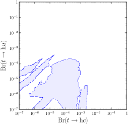
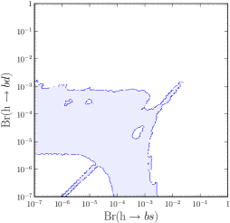
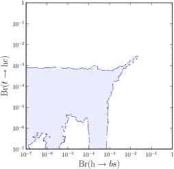
CFTP/18-012

IFIC/18-nnn

Vacuum Induced CP Violation Generating a Complex CKM Matrix with Controlled Scalar FCNC

Miguel Nebot a,111miguel.r.nebot.gomez@tecnico.ulisboa.pt Francisco J. Botella b,222Francisco.J.Botella@uv.es, Gustavo C. Branco a,333gbranco@tecnico.ulisboa.pt,

a Departamento de Física and Centro de Física Teórica de Partículas (CFTP),
 Instituto Superior Técnico (IST), U. de Lisboa (UL),
 Av. Rovisco Pais 1, P-1049-001 Lisboa, Portugal.

b Departament de Fìsica Teòrica and Instituto de Física Corpuscular (IFIC),
 Universitat de València – CSIC, E-46100 Valencia, Spain.

Abstract

We propose a viable minimal model with spontaneous CP violation in the framework of a Two Higgs Doublet Model. The model is based on a generalised Branco-Grimus-Lavoura model with a flavoured 2subscript2\mathbb{Z}_{2} symmetry, under which two of the quark families are even and the third one is odd. The lagrangian respects CP invariance, but the vacuum has a CP violating phase, which is able to generate a complex CKM matrix, with the rephasing invariant strength of CP violation compatible with experiment. The question of scalar mediated flavour changing neutral couplings is carefully studied. In particular we point out a deep connection between the generation of a complex CKM matrix from a vacuum phase and the appearance of scalar FCNC. The scalar sector is presented in detail, showing that the new scalars are necessarily lighter than 1 TeV. A complete analysis of the model including the most relevant constraints is performed, showing that it is viable and that it has definite implications for the observation of New Physics signals in, for example, flavour changing Higgs decays or the discovery of the new scalars at the LHC. We give special emphasis to processes like thc,hu𝑡h𝑐h𝑢t\to{\rm h}c,{\rm h}u, as well as hbs,bdh𝑏𝑠𝑏𝑑{\rm h}\to bs,bd, which are relevant for the LHC and the ILC.

1 Introduction

The first model of spontaneous T and CP violation was proposed [1] by T.D. Lee in 1973 at a time when only two incomplete quark generations were known. The main motivation for Lee’s seminal work was to put the breaking of CP and T on the same footing as the breaking of gauge symmetry. In Lee’s model, the Lagrangian is CP and T invariant, but the vacuum violates these discrete symmetries. This was achieved through the introduction of two Higgs doublets, with vacuum expectation values with a relative phase which violates T and CP invariance. In Lee’s model, CP violation would arise solely from Higgs exchange, since at the time only two generations were known and therefore the CKM matrix was real. The general two Higgs Doublet Model (2HDM) [2, 3] has Scalar Flavour Changing Neutral Couplings (SFCNC) at tree level which need to be controlled in order to conform to the stringent experimental constraints. This can be achieved by imposing Natural Flavour Conservation (NFC) in the scalar sector, as suggested by Glashow and Weinberg (GW) [4]. Alternatively, it was suggested by Branco, Grimus and Lavoura (BGL) [5] that one may have 2HDM with tree level SFCNC but with their flavour structure only dependent on the CKM matrix V𝑉V.

BGL models have been extensively analysed in the literature [6, 7, 8, 9, 10, 11], and their phenomenological consequences have been studied, in particular in the context of LHC. Recently BGL models have been generalised [12] in the framework of 2HDM. Both the GW and the BGL schemes can be implemented through the introduction of extra symmetries in the 2HDM. On the other hand, it has been shown [13] that the introduction of these symmetries in the 2HDM prevents the generation of either spontaneous or explicit CP violation in the scalar sector, unless they are softly broken [14]. It was recently discussed [15] that for a scalar potential with an extra symmetry beyond gauge symmetry, there is an intriguing correlation between the capability of the potential to generate explicit and spontaneous CP violation.

In this paper we propose a realistic model of spontaneous CP violation in the framework of 2HDM. At this stage it is worth recalling the obstacles which have to be surmounted by any model of spontaneous CP violation:

  • (i)

    The scalar potential should be able to generate spontaneous CP breaking by a phase of the vacuum, denoted θ𝜃\theta.

  • (ii)

    The phase θ𝜃\theta should be able to generate a complex CKM matrix, with the strength of CP violation compatible with experiment. Recall that the CKM matrix has to be complex even in the presence of New Physics [16].

  • (iii)

    SFCNC effects should be under control so that they do not violate experimental bounds.

The paper is organised as follows. In the next section we present the structure of the model and specify the flavoured symmetry introduced. In the third section we show how a complex CKM matrix is generated from the vacuum phase. Section 4 contains a detailed analysis of the scalar potential with real couplings. In section 5 we derive the physical Yukawa couplings and the phenomenological analysis of the model is presented in section 6. Finally we present our conclusions in the last section.

2 The Structure of the Model and the Flavoured symmetry

The Yukawa couplings in the 2HDM read

Y=Q¯L0(Γ1Φ1+Γ2Φ2)dR0Q¯L0(Δ1Φ~1+Δ2Φ~2)uR0+H.c.,subscriptYsuperscriptsubscript¯𝑄𝐿0subscriptΓ1superscriptsubscriptΦ1absentsubscriptΓ2superscriptsubscriptΦ2absentsuperscriptsubscript𝑑𝑅0superscriptsubscript¯𝑄𝐿0subscriptΔ1superscriptsubscript~Φ1absentsubscriptΔ2superscriptsubscript~Φ2absentsuperscriptsubscript𝑢𝑅0H.c.\mathscr{L}_{\rm Y}=-\bar{Q}_{L}^{0}(\Gamma_{1}\Phi_{1}^{\phantom{\dagger}}+\Gamma_{2}\Phi_{2}^{\phantom{\dagger}})d_{R}^{0}-\bar{Q}_{L}^{0}(\Delta_{1}\tilde{\Phi}_{1}^{\phantom{\dagger}}+\Delta_{2}\tilde{\Phi}_{2}^{\phantom{\dagger}})u_{R}^{0}+\text{H.c.}\,, (1)

with summation over generation indices understood and Φ~j=iσ2Φjsuperscriptsubscript~Φ𝑗absent𝑖subscript𝜎2superscriptsubscriptΦ𝑗\tilde{\Phi}_{j}^{\phantom{\dagger}}=i\sigma_{2}\Phi_{j}^{\phantom{\dagger}\!\!\!\ast}. We consider the following 2subscript2\mathbb{Z}_{2} transformations to define the model:

Φ1Φ1,Φ2Φ2,QL30QL30,QLj0QLj0,j=1,2,formulae-sequencemaps-tosuperscriptsubscriptΦ1absentsuperscriptsubscriptΦ1absentformulae-sequencemaps-tosuperscriptsubscriptΦ2absentsuperscriptsubscriptΦ2absentformulae-sequencemaps-tosuperscriptsubscript𝑄𝐿30superscriptsubscript𝑄𝐿30formulae-sequencemaps-tosuperscriptsubscript𝑄𝐿𝑗0superscriptsubscript𝑄𝐿𝑗0𝑗12\displaystyle\Phi_{1}^{\phantom{\dagger}}\mapsto\Phi_{1}^{\phantom{\dagger}},\quad\Phi_{2}^{\phantom{\dagger}}\mapsto-\Phi_{2}^{\phantom{\dagger}},\quad Q_{L3}^{0}\mapsto-Q_{L3}^{0},\quad Q_{Lj}^{0}\mapsto Q_{Lj}^{0},\quad j=1,2,
dRk0dRk0,uRk0uRk0,k=1,2,3.formulae-sequencemaps-tosuperscriptsubscript𝑑𝑅𝑘0superscriptsubscript𝑑𝑅𝑘0formulae-sequencemaps-tosuperscriptsubscript𝑢𝑅𝑘0superscriptsubscript𝑢𝑅𝑘0𝑘123\displaystyle d_{Rk}^{0}\mapsto d_{Rk}^{0},\quad u_{Rk}^{0}\mapsto u_{Rk}^{0},\quad k=1,2,3. (2)

Invariance under eq. (2) gives the following form of the Yukawa coupling matrices:

Γ1=(××××××000),subscriptΓ1matrix000\displaystyle\Gamma_{1}=\begin{pmatrix}\times&\times&\times\\ \times&\times&\times\\ 0&0&0\end{pmatrix}, Γ2=(000000×××),subscriptΓ2matrix000000\displaystyle\Gamma_{2}=\begin{pmatrix}0&0&0\\ 0&0&0\\ \times&\times&\times\end{pmatrix},
Δ1=(××××××000),subscriptΔ1matrix000\displaystyle\Delta_{1}=\begin{pmatrix}\times&\times&\times\\ \times&\times&\times\\ 0&0&0\end{pmatrix}, Δ2=(000000×××).subscriptΔ2matrix000000\displaystyle\Delta_{2}=\begin{pmatrix}0&0&0\\ 0&0&0\\ \times&\times&\times\end{pmatrix}. (3)

The symmetry assignment in eq. (2) and the Yukawa matrices in eq. (3) correspond to the generalised BGL models introduced in [12]. We impose CP invariance at the Lagrangian level, so we require the Yukawa couplings to be real:

Γj=Γj,Δj=Δj.formulae-sequencesuperscriptsubscriptΓ𝑗subscriptΓ𝑗superscriptsubscriptΔ𝑗subscriptΔ𝑗\Gamma_{j}^{\ast}=\Gamma_{j},\qquad\Delta_{j}^{\ast}=\Delta_{j}\,. (4)

We write the scalar doublets ΦjsuperscriptsubscriptΦ𝑗absent\Phi_{j}^{\phantom{\dagger}} in the “Higgs basis” {H1,H2}subscript𝐻1subscript𝐻2\{H_{1},H_{2}\} [17, 18, 19] (see section 4 and appendix B for further details on the scalar sector)

(H1H2)=β(eiθ1Φ1eiθ2Φ2),withβ=(cβsβsβcβ),βT=β1.formulae-sequencematrixsubscript𝐻1subscript𝐻2superscriptsubscript𝛽absentmatrixsuperscript𝑒𝑖subscript𝜃1superscriptsubscriptΦ1absentsuperscript𝑒𝑖subscript𝜃2superscriptsubscriptΦ2absentwithformulae-sequencesuperscriptsubscript𝛽absentmatrixsubscript𝑐𝛽subscript𝑠𝛽subscript𝑠𝛽subscript𝑐𝛽superscriptsubscript𝛽𝑇superscriptsubscript𝛽1\begin{pmatrix}H_{1}\\ H_{2}\end{pmatrix}=\mathcal{R}_{\beta}^{\phantom{T}}\,\begin{pmatrix}e^{-i\theta_{1}}\Phi_{1}^{\phantom{\dagger}}\\ e^{-i\theta_{2}}\Phi_{2}^{\phantom{\dagger}}\end{pmatrix},\quad\text{with}\quad\mathcal{R}_{\beta}^{\phantom{T}}=\begin{pmatrix}\phantom{-}c_{\beta}&s_{\beta}\\ -s_{\beta}&c_{\beta}\end{pmatrix},\ \mathcal{R}_{\beta}^{T}=\mathcal{R}_{\beta}^{-1}. (5)

In this basis, only H1subscript𝐻1H_{1} acquires a vacuum expectation value

H1=v2(01),H2=(00).formulae-sequencedelimited-⟨⟩subscript𝐻1𝑣2matrix01delimited-⟨⟩subscript𝐻2matrix00\langle H_{1}\rangle=\frac{v}{\sqrt{2}}\begin{pmatrix}0\\ 1\end{pmatrix},\quad\langle H_{2}\rangle=\begin{pmatrix}0\\ 0\end{pmatrix}. (6)

Equation (1) can then be rewritten as

Y=2vQ¯L0(Md0H1+Nd0H2)dR02vQ¯L0(Mu0H~1+Nu0H~2)uR0+H.c.,subscriptY2𝑣superscriptsubscript¯𝑄𝐿0superscriptsubscript𝑀𝑑0subscript𝐻1superscriptsubscript𝑁𝑑0subscript𝐻2superscriptsubscript𝑑𝑅02𝑣superscriptsubscript¯𝑄𝐿0superscriptsubscript𝑀𝑢0subscript~𝐻1superscriptsubscript𝑁𝑢0subscript~𝐻2superscriptsubscript𝑢𝑅0H.c.\mathscr{L}_{\rm Y}=-\frac{\sqrt{2}}{v}\bar{Q}_{L}^{0}(M_{d}^{0}H_{1}+N_{d}^{0}H_{2})d_{R}^{0}-\frac{\sqrt{2}}{v}\bar{Q}_{L}^{0}(M_{u}^{0}\tilde{H}_{1}+N_{u}^{0}\tilde{H}_{2})u_{R}^{0}+\text{H.c.}\,, (7)

where the quark mass matrices Md0superscriptsubscript𝑀𝑑0M_{d}^{0}, Mu0superscriptsubscript𝑀𝑢0M_{u}^{0} and the Nd0superscriptsubscript𝑁𝑑0N_{d}^{0}, Nu0superscriptsubscript𝑁𝑢0N_{u}^{0} matrices read

Md0superscriptsubscript𝑀𝑑0\displaystyle M_{d}^{0} =veiθ12(cβΓ1+eiθsβΓ2),absent𝑣superscript𝑒𝑖subscript𝜃12subscript𝑐𝛽subscriptΓ1superscript𝑒𝑖𝜃subscript𝑠𝛽subscriptΓ2\displaystyle=\frac{ve^{i\theta_{1}}}{\sqrt{2}}(c_{\beta}\Gamma_{1}+e^{i\theta}s_{\beta}\Gamma_{2})\,, Nd0superscriptsubscript𝑁𝑑0\displaystyle\quad N_{d}^{0} =veiθ12(sβΓ1+eiθcβΓ2),absent𝑣superscript𝑒𝑖subscript𝜃12subscript𝑠𝛽subscriptΓ1superscript𝑒𝑖𝜃subscript𝑐𝛽subscriptΓ2\displaystyle=\frac{ve^{i\theta_{1}}}{\sqrt{2}}(-s_{\beta}\Gamma_{1}+e^{i\theta}c_{\beta}\Gamma_{2})\,, (8)
Mu0superscriptsubscript𝑀𝑢0\displaystyle M_{u}^{0} =veiθ12(cβΔ1+eiθsβΔ2),absent𝑣superscript𝑒𝑖subscript𝜃12subscript𝑐𝛽subscriptΔ1superscript𝑒𝑖𝜃subscript𝑠𝛽subscriptΔ2\displaystyle=\frac{ve^{-i\theta_{1}}}{\sqrt{2}}(c_{\beta}\Delta_{1}+e^{-i\theta}s_{\beta}\Delta_{2})\,, Nu0superscriptsubscript𝑁𝑢0\displaystyle\quad N_{u}^{0} =veiθ12(sβΔ1+eiθcβΔ2),absent𝑣superscript𝑒𝑖subscript𝜃12subscript𝑠𝛽subscriptΔ1superscript𝑒𝑖𝜃subscript𝑐𝛽subscriptΔ2\displaystyle=\frac{ve^{-i\theta_{1}}}{\sqrt{2}}(-s_{\beta}\Delta_{1}+e^{-i\theta}c_{\beta}\Delta_{2})\,, (9)

where θ=θ2θ1𝜃subscript𝜃2subscript𝜃1\theta=\theta_{2}-\theta_{1} is the relative phase among Φ2delimited-⟨⟩superscriptsubscriptΦ2absent\langle\Phi_{2}^{\phantom{\dagger}}\rangle and Φ1delimited-⟨⟩superscriptsubscriptΦ1absent\langle\Phi_{1}^{\phantom{\dagger}}\rangle. For simplicity, we remove the irrelevant global phases e±iθ1superscript𝑒plus-or-minus𝑖subscript𝜃1e^{\pm i\theta_{1}} setting θ1=0subscript𝜃10\theta_{1}=0.
Notice that the matrices Nd0superscriptsubscript𝑁𝑑0N_{d}^{0}, Nu0superscriptsubscript𝑁𝑢0N_{u}^{0} can be written:

Nd0superscriptsubscript𝑁𝑑0\displaystyle N_{d}^{0} =tβMd0+eiθv2(tβ+tβ1)sβΓ2=tβMd0(tβ+tβ1)P3Md0,absentsubscript𝑡𝛽superscriptsubscript𝑀𝑑0superscript𝑒𝑖𝜃𝑣2subscript𝑡𝛽superscriptsubscript𝑡𝛽1subscript𝑠𝛽subscriptΓ2subscript𝑡𝛽superscriptsubscript𝑀𝑑0subscript𝑡𝛽superscriptsubscript𝑡𝛽1subscriptP3superscriptsubscript𝑀𝑑0\displaystyle=t_{\beta}M_{d}^{0}+e^{i\theta}\frac{v}{\sqrt{2}}(t_{\beta}+t_{\beta}^{-1})s_{\beta}\Gamma_{2}=t_{\beta}M_{d}^{0}-(t_{\beta}+t_{\beta}^{-1}){\rm P}_{\!3}M_{d}^{0}\,, (10)
Nu0superscriptsubscript𝑁𝑢0\displaystyle N_{u}^{0} =tβMu0+eiθv2(tβ+tβ1)sβΔ2=tβMu0(tβ+tβ1)P3Mu0,absentsubscript𝑡𝛽superscriptsubscript𝑀𝑢0superscript𝑒𝑖𝜃𝑣2subscript𝑡𝛽superscriptsubscript𝑡𝛽1subscript𝑠𝛽subscriptΔ2subscript𝑡𝛽superscriptsubscript𝑀𝑢0subscript𝑡𝛽superscriptsubscript𝑡𝛽1subscriptP3superscriptsubscript𝑀𝑢0\displaystyle=t_{\beta}M_{u}^{0}+e^{-i\theta}\frac{v}{\sqrt{2}}(t_{\beta}+t_{\beta}^{-1})s_{\beta}\Delta_{2}=t_{\beta}M_{u}^{0}-(t_{\beta}+t_{\beta}^{-1}){\rm P}_{\!3}M_{u}^{0}\,, (11)

where P3subscriptP3{\rm P}_{\!3} is the projector

P3=(000000001).subscriptP3matrix000000001{\rm P}_{\!3}=\begin{pmatrix}0&0&0\\ 0&0&0\\ 0&0&1\end{pmatrix}\,. (12)

3 Generation of a complex CKM matrix from the vacuum phase

In this section, we show how the vacuum phase θ𝜃\theta is capable of generating a complex CKM matrix. As previously emphasized, this is a necessary requirement for the model to be consistent with experiment. Following eqs. (3)-(4) and (8)-(9), we write:

Md0=(10001000eiθ)M^d0,Mu0=(10001000eiθ)M^u0,formulae-sequencesuperscriptsubscript𝑀𝑑0matrix10001000superscript𝑒𝑖𝜃superscriptsubscript^𝑀𝑑0superscriptsubscript𝑀𝑢0matrix10001000superscript𝑒𝑖𝜃superscriptsubscript^𝑀𝑢0M_{d}^{0}=\begin{pmatrix}1&0&0\\ 0&1&0\\ 0&0&e^{i\theta}\end{pmatrix}\hat{M}_{d}^{0},\qquad M_{u}^{0}=\begin{pmatrix}1&0&0\\ 0&1&0\\ 0&0&e^{-i\theta}\end{pmatrix}\hat{M}_{u}^{0}, (13)

with M^d0superscriptsubscript^𝑀𝑑0\hat{M}_{d}^{0} and M^u0superscriptsubscript^𝑀𝑢0\hat{M}_{u}^{0} real. Then,

Md0Md0=(10001000eiθ)M^d0M^d0T(10001000eiθ)superscriptsubscript𝑀𝑑0superscriptsubscript𝑀𝑑0matrix10001000superscript𝑒𝑖𝜃superscriptsubscript^𝑀𝑑0superscriptsubscript^𝑀𝑑0𝑇matrix10001000superscript𝑒𝑖𝜃M_{d}^{0}M_{d}^{0\dagger}=\begin{pmatrix}1&0&0\\ 0&1&0\\ 0&0&e^{i\theta}\end{pmatrix}\hat{M}_{d}^{0}\hat{M}_{d}^{0\,T}\begin{pmatrix}1&0&0\\ 0&1&0\\ 0&0&e^{-i\theta}\end{pmatrix} (14)

with M^d0M^d0Tsuperscriptsubscript^𝑀𝑑0superscriptsubscript^𝑀𝑑0𝑇\hat{M}_{d}^{0}\hat{M}_{d}^{0\,T} real and symmetric, which is diagonalised with a real orthogonal transformation:

𝒪LdTM^d0M^d0T𝒪Ld=diag(mdi2).superscriptsubscript𝒪𝐿𝑑𝑇superscriptsubscript^𝑀𝑑0superscriptsubscript^𝑀𝑑0𝑇superscriptsubscript𝒪𝐿𝑑diagsuperscriptsubscript𝑚subscript𝑑𝑖2\mathcal{O}_{L}^{d\,T}\,\hat{M}_{d}^{0}\hat{M}_{d}^{0\,T}\,\mathcal{O}_{L}^{d}=\text{diag}(m_{d_{i}}^{2})\,. (15)

Consequently, eq. (14) gives

𝒪LdT(10001000eiθ)Md0Md0(10001000eiθ)𝒪Ld=diag(mdi2).superscriptsubscript𝒪𝐿𝑑𝑇matrix10001000superscript𝑒𝑖𝜃superscriptsubscript𝑀𝑑0superscriptsubscript𝑀𝑑0matrix10001000superscript𝑒𝑖𝜃superscriptsubscript𝒪𝐿𝑑diagsuperscriptsubscript𝑚subscript𝑑𝑖2\mathcal{O}_{L}^{d\,T}\begin{pmatrix}1&0&0\\ 0&1&0\\ 0&0&e^{-i\theta}\end{pmatrix}M_{d}^{0}M_{d}^{0\dagger}\begin{pmatrix}1&0&0\\ 0&1&0\\ 0&0&e^{i\theta}\end{pmatrix}\mathcal{O}_{L}^{d}=\text{diag}(m_{d_{i}}^{2})\,. (16)

That is, the diagonalisation of Md0Md0superscriptsubscript𝑀𝑑0superscriptsubscript𝑀𝑑0M_{d}^{0}M_{d}^{0\dagger} is accomplished with

𝒰LdMd0Md0𝒰Ld=diag(mdi2),where𝒰Ld=(10001000eiθ)𝒪Ld.formulae-sequencesuperscriptsubscript𝒰𝐿𝑑superscriptsubscript𝑀𝑑0superscriptsubscript𝑀𝑑0superscriptsubscript𝒰𝐿𝑑diagsuperscriptsubscript𝑚subscript𝑑𝑖2wheresuperscriptsubscript𝒰𝐿𝑑matrix10001000superscript𝑒𝑖𝜃superscriptsubscript𝒪𝐿𝑑\mathcal{U}_{L}^{d\dagger}M_{d}^{0}M_{d}^{0\dagger}\mathcal{U}_{L}^{d}=\text{diag}(m_{d_{i}}^{2})\,,\quad\text{where}\quad\mathcal{U}_{L}^{d}=\begin{pmatrix}1&0&0\\ 0&1&0\\ 0&0&e^{i\theta}\end{pmatrix}\mathcal{O}_{L}^{d}\,. (17)

Similarly,

𝒰LuMu0Mu0𝒰Lu=diag(mui2),with𝒰Lu=(10001000eiθ)𝒪Lu.formulae-sequencesuperscriptsubscript𝒰𝐿𝑢superscriptsubscript𝑀𝑢0superscriptsubscript𝑀𝑢0superscriptsubscript𝒰𝐿𝑢diagsuperscriptsubscript𝑚subscript𝑢𝑖2withsuperscriptsubscript𝒰𝐿𝑢matrix10001000superscript𝑒𝑖𝜃superscriptsubscript𝒪𝐿𝑢\mathcal{U}_{L}^{u\dagger}M_{u}^{0}M_{u}^{0\dagger}\mathcal{U}_{L}^{u}=\text{diag}(m_{u_{i}}^{2})\,,\quad\text{with}\quad\mathcal{U}_{L}^{u}=\begin{pmatrix}1&0&0\\ 0&1&0\\ 0&0&e^{-i\theta}\end{pmatrix}\mathcal{O}_{L}^{u}\,. (18)

Notice the important sign difference in θ𝜃\theta between eqs. (17) and (18), which give the following CKM matrix V𝒰Lu𝒰Ld𝑉superscriptsubscript𝒰𝐿𝑢superscriptsubscript𝒰𝐿𝑑V\equiv\mathcal{U}_{L}^{u\dagger}\mathcal{U}_{L}^{d},

V=𝒪LuT(10001000ei2θ)𝒪Ld.𝑉superscriptsubscript𝒪𝐿𝑢𝑇matrix10001000superscript𝑒𝑖2𝜃superscriptsubscript𝒪𝐿𝑑V=\mathcal{O}_{L}^{u\,T}\begin{pmatrix}1&0&0\\ 0&1&0\\ 0&0&e^{i2\theta}\end{pmatrix}\mathcal{O}_{L}^{d}\,. (19)

Notice also that, if ei2θ=±1superscript𝑒𝑖2𝜃plus-or-minus1e^{i2\theta}=\pm 1, V𝑉V is real, i.e. it does not generate CP violation. This can be understood through a careful analysis of the potential, which will be presented in section 4. The model we present here has spontaneous CP violation and thus a physical phase in the CKM matrix can only arise from θ𝜃\theta. In section 4.1 we show that for θ=π/2𝜃𝜋2\theta=\pi/2 the vacuum is CP invariant and no CP violation can be generated in this model. In particular CKM is necessarily real for this value of θ𝜃\theta, as noticed in eq. (19).

It is also straightforward to observe that Md0Md0superscriptsubscript𝑀𝑑0superscriptsubscript𝑀𝑑0M_{d}^{0\dagger}M_{d}^{0} and Mu0Mu0superscriptsubscript𝑀𝑢0superscriptsubscript𝑀𝑢0M_{u}^{0\dagger}M_{u}^{0} are real and symmetric, and are thus diagonalised with real orthogonal matrices 𝒪Rdsuperscriptsubscript𝒪𝑅𝑑\mathcal{O}_{R}^{d} and 𝒪Rusuperscriptsubscript𝒪𝑅𝑢\mathcal{O}_{R}^{u},

𝒪RdTMd0Md0𝒪Rd=diag(mdi2),𝒪RuTMu0Mu0𝒪Ru=diag(mui2),formulae-sequencesuperscriptsubscript𝒪𝑅𝑑𝑇superscriptsubscript𝑀𝑑0superscriptsubscript𝑀𝑑0superscriptsubscript𝒪𝑅𝑑diagsuperscriptsubscript𝑚subscript𝑑𝑖2superscriptsubscript𝒪𝑅𝑢𝑇superscriptsubscript𝑀𝑢0superscriptsubscript𝑀𝑢0superscriptsubscript𝒪𝑅𝑢diagsuperscriptsubscript𝑚subscript𝑢𝑖2\mathcal{O}_{R}^{d\,T}M_{d}^{0\dagger}M_{d}^{0}\mathcal{O}_{R}^{d}=\text{diag}(m_{d_{i}}^{2}),\qquad\mathcal{O}_{R}^{u\,T}M_{u}^{0\dagger}M_{u}^{0}\mathcal{O}_{R}^{u}=\text{diag}(m_{u_{i}}^{2})\,, (20)

such that the bi-diagonalisation of Md0superscriptsubscript𝑀𝑑0M_{d}^{0} and Mu0superscriptsubscript𝑀𝑢0M_{u}^{0} reads

Md=diag(mdi)=𝒰LdMd0𝒪Rd,Mu=diag(mui)=𝒰LuMu0𝒪Ru.formulae-sequencesuperscriptsubscript𝑀𝑑absentdiagsubscript𝑚subscript𝑑𝑖superscriptsubscript𝒰𝐿𝑑superscriptsubscript𝑀𝑑0superscriptsubscript𝒪𝑅𝑑superscriptsubscript𝑀𝑢absentdiagsubscript𝑚subscript𝑢𝑖superscriptsubscript𝒰𝐿𝑢superscriptsubscript𝑀𝑢0superscriptsubscript𝒪𝑅𝑢M_{d}^{\phantom{\dagger}}=\text{diag}(m_{d_{i}})=\mathcal{U}_{L}^{d\dagger}M_{d}^{0}\mathcal{O}_{R}^{d},\quad M_{u}^{\phantom{\dagger}}=\text{diag}(m_{u_{i}})=\mathcal{U}_{L}^{u\dagger}M_{u}^{0}\mathcal{O}_{R}^{u}\,. (21)

Following eq. (10),

Nd𝒰LdNd0𝒪Rd=tβ𝒰LdMd0𝒪Rd(tβ+tβ1)𝒰LdP3Md0𝒪Rd=tβMd(tβ+tβ1)𝒰LdP3𝒰LdMd,superscriptsubscript𝑁𝑑absentsuperscriptsubscript𝒰𝐿𝑑superscriptsubscript𝑁𝑑0superscriptsubscript𝒪𝑅𝑑subscript𝑡𝛽superscriptsubscript𝒰𝐿𝑑superscriptsubscript𝑀𝑑0superscriptsubscript𝒪𝑅𝑑subscript𝑡𝛽superscriptsubscript𝑡𝛽1superscriptsubscript𝒰𝐿𝑑subscriptP3superscriptsubscript𝑀𝑑0superscriptsubscript𝒪𝑅𝑑subscript𝑡𝛽superscriptsubscript𝑀𝑑absentsubscript𝑡𝛽superscriptsubscript𝑡𝛽1superscriptsubscript𝒰𝐿𝑑subscriptP3superscriptsubscript𝒰𝐿𝑑superscriptsubscript𝑀𝑑absentN_{d}^{\phantom{\dagger}}\equiv\mathcal{U}_{L}^{d\dagger}N_{d}^{0}\mathcal{O}_{R}^{d}=t_{\beta}\mathcal{U}_{L}^{d\dagger}M_{d}^{0}\mathcal{O}_{R}^{d}-(t_{\beta}+t_{\beta}^{-1})\mathcal{U}_{L}^{d\dagger}{\rm P}_{\!3}M_{d}^{0}\mathcal{O}_{R}^{d}=\\ t_{\beta}M_{d}^{\phantom{\dagger}}-(t_{\beta}+t_{\beta}^{-1})\mathcal{U}_{L}^{d\dagger}{\rm P}_{\!3}\mathcal{U}_{L}^{d}M_{d}^{\phantom{\dagger}}\,, (22)

with P3subscriptP3{\rm P}_{\!3} the projector in eq. (12) and 𝒰Ldsuperscriptsubscript𝒰𝐿𝑑\mathcal{U}_{L}^{d} in eq. (17). In the last term of eq. (22),

𝒰LdP3𝒰Ld=𝒪LdTP3𝒪Ld,superscriptsubscript𝒰𝐿𝑑subscriptP3superscriptsubscript𝒰𝐿𝑑superscriptsubscript𝒪𝐿𝑑𝑇subscriptP3superscriptsubscript𝒪𝐿𝑑\mathcal{U}_{L}^{d\dagger}{\rm P}_{\!3}\mathcal{U}_{L}^{d}=\mathcal{O}_{L}^{d\,T}{\rm P}_{\!3}\mathcal{O}_{L}^{d}\,, (23)

that is, Ndsuperscriptsubscript𝑁𝑑absentN_{d}^{\phantom{\dagger}} in eq. (22) is real. Introducing a real unit vector r^[d]subscript^𝑟delimited-[]d\hat{r}_{{\rm[d]}} and a complex unit vector n^[d]superscriptsubscript^𝑛delimited-[]dabsent\hat{n}_{{\rm[d]}}^{\phantom{\ast}} with components

r^[d]j[𝒪Ld]3j,n^[d]j[𝒰Ld]3j=eiθr^[d]j,formulae-sequencesubscript^𝑟delimited-[]d𝑗subscriptdelimited-[]superscriptsubscript𝒪𝐿𝑑3𝑗superscriptsubscript^𝑛delimited-[]d𝑗absentsubscriptdelimited-[]superscriptsubscript𝒰𝐿𝑑3𝑗superscript𝑒𝑖𝜃subscript^𝑟delimited-[]d𝑗\hat{r}_{{\rm[d]}j}\equiv[\mathcal{O}_{L}^{d}]_{3j}\,,\quad\hat{n}_{{\rm[d]}j}^{\phantom{\ast}}\equiv[\mathcal{U}_{L}^{d}]_{3j}=e^{i\theta}\hat{r}_{{\rm[d]}j}\,, (24)

one has, for 𝒰LdP3𝒰Ldsuperscriptsubscript𝒰𝐿𝑑subscriptP3superscriptsubscript𝒰𝐿𝑑\mathcal{U}_{L}^{d\dagger}{\rm P}_{\!3}\mathcal{U}_{L}^{d} in eq. (23),

[𝒰LdP3𝒰Ld]ij=n^[d]in^[d]j=r^[d]ir^[d]j.subscriptdelimited-[]superscriptsubscript𝒰𝐿𝑑subscriptP3superscriptsubscript𝒰𝐿𝑑𝑖𝑗superscriptsubscript^𝑛delimited-[]d𝑖superscriptsubscript^𝑛delimited-[]d𝑗absentsubscript^𝑟delimited-[]d𝑖subscript^𝑟delimited-[]d𝑗[\mathcal{U}_{L}^{d\dagger}{\rm P}_{\!3}\mathcal{U}_{L}^{d}]_{ij}=\hat{n}_{{\rm[d]}i}^{\ast}\hat{n}_{{\rm[d]}j}^{\phantom{\ast}}=\hat{r}_{{\rm[d]}i}\hat{r}_{{\rm[d]}j}\,. (25)

Similarly, for Nusuperscriptsubscript𝑁𝑢absentN_{u}^{\phantom{\dagger}} we have

Nu𝒰LuNu0𝒪Ru=tβMu(tβ+tβ1)𝒰LuP3𝒰LuMu,superscriptsubscript𝑁𝑢absentsuperscriptsubscript𝒰𝐿𝑢superscriptsubscript𝑁𝑢0superscriptsubscript𝒪𝑅𝑢subscript𝑡𝛽superscriptsubscript𝑀𝑢absentsubscript𝑡𝛽superscriptsubscript𝑡𝛽1superscriptsubscript𝒰𝐿𝑢subscriptP3superscriptsubscript𝒰𝐿𝑢superscriptsubscript𝑀𝑢absentN_{u}^{\phantom{\dagger}}\equiv\mathcal{U}_{L}^{u\dagger}N_{u}^{0}\mathcal{O}_{R}^{u}=t_{\beta}M_{u}^{\phantom{\dagger}}-(t_{\beta}+t_{\beta}^{-1})\mathcal{U}_{L}^{u\dagger}{\rm P}_{\!3}\mathcal{U}_{L}^{u}M_{u}^{\phantom{\dagger}}\,, (26)

with

𝒰LuP3𝒰Lu=𝒪LuTP3𝒪Lu,superscriptsubscript𝒰𝐿𝑢subscriptP3superscriptsubscript𝒰𝐿𝑢superscriptsubscript𝒪𝐿𝑢𝑇subscriptP3superscriptsubscript𝒪𝐿𝑢\mathcal{U}_{L}^{u\dagger}{\rm P}_{\!3}\mathcal{U}_{L}^{u}=\mathcal{O}_{L}^{u\,T}{\rm P}_{\!3}\mathcal{O}_{L}^{u}\,, (27)

and

r^[u]j[𝒪Lu]3jn^[u]j[𝒰Lu]3j=eiθr^[u]j,[𝒰LuP3𝒰Lu]ij=n^[u]in^[u]j=r^[u]ir^[u]j.formulae-sequenceformulae-sequencesubscript^𝑟delimited-[]u𝑗subscriptdelimited-[]superscriptsubscript𝒪𝐿𝑢3𝑗superscriptsubscript^𝑛delimited-[]u𝑗absentsubscriptdelimited-[]superscriptsubscript𝒰𝐿𝑢3𝑗superscript𝑒𝑖𝜃subscript^𝑟delimited-[]u𝑗subscriptdelimited-[]superscriptsubscript𝒰𝐿𝑢subscriptP3superscriptsubscript𝒰𝐿𝑢𝑖𝑗superscriptsubscript^𝑛delimited-[]u𝑖superscriptsubscript^𝑛delimited-[]u𝑗absentsubscript^𝑟delimited-[]u𝑖subscript^𝑟delimited-[]u𝑗\hat{r}_{{\rm[u]}j}\equiv[\mathcal{O}_{L}^{u}]_{3j}\,\quad\hat{n}_{{\rm[u]}j}^{\phantom{\ast}}\equiv[\mathcal{U}_{L}^{u}]_{3j}=e^{-i\theta}\hat{r}_{{\rm[u]}j}\,,\quad[\mathcal{U}_{L}^{u\dagger}{\rm P}_{\!3}\mathcal{U}_{L}^{u}]_{ij}=\hat{n}_{{\rm[u]}i}^{\ast}\hat{n}_{{\rm[u]}j}^{\phantom{\ast}}=\hat{r}_{{\rm[u]}i}\hat{r}_{{\rm[u]}j}\,. (28)

Like Ndsuperscriptsubscript𝑁𝑑absentN_{d}^{\phantom{\dagger}}, Nusuperscriptsubscript𝑁𝑢absentN_{u}^{\phantom{\dagger}} is real; Ndsuperscriptsubscript𝑁𝑑absentN_{d}^{\phantom{\dagger}} and Nusuperscriptsubscript𝑁𝑢absentN_{u}^{\phantom{\dagger}} have the form:

[Nd]ijsubscriptdelimited-[]superscriptsubscript𝑁𝑑absent𝑖𝑗\displaystyle[N_{d}^{\phantom{\dagger}}]_{ij} =tβδijmdi(tβ+tβ1)n^[d]in^[d]jmdj,absentsubscript𝑡𝛽subscript𝛿𝑖𝑗subscript𝑚subscript𝑑𝑖subscript𝑡𝛽superscriptsubscript𝑡𝛽1superscriptsubscript^𝑛delimited-[]d𝑖superscriptsubscript^𝑛delimited-[]d𝑗absentsubscript𝑚subscript𝑑𝑗\displaystyle=t_{\beta}\delta_{ij}m_{d_{i}}-(t_{\beta}+t_{\beta}^{-1})\hat{n}_{{\rm[d]}i}^{\ast}\hat{n}_{{\rm[d]}j}^{\phantom{\ast}}m_{d_{j}}\,, (29)
[Nu]ijsubscriptdelimited-[]superscriptsubscript𝑁𝑢absent𝑖𝑗\displaystyle[N_{u}^{\phantom{\dagger}}]_{ij} =tβδijmui(tβ+tβ1)n^[u]in^[u]jmuj.absentsubscript𝑡𝛽subscript𝛿𝑖𝑗subscript𝑚subscript𝑢𝑖subscript𝑡𝛽superscriptsubscript𝑡𝛽1superscriptsubscript^𝑛delimited-[]u𝑖superscriptsubscript^𝑛delimited-[]u𝑗absentsubscript𝑚subscript𝑢𝑗\displaystyle=t_{\beta}\delta_{ij}m_{u_{i}}-(t_{\beta}+t_{\beta}^{-1})\hat{n}_{{\rm[u]}i}^{\ast}\hat{n}_{{\rm[u]}j}^{\phantom{\ast}}m_{u_{j}}\,. (30)

Since V=𝒰Lu𝒰Ld𝑉superscriptsubscript𝒰𝐿𝑢superscriptsubscript𝒰𝐿𝑑V=\mathcal{U}_{L}^{u\dagger}\mathcal{U}_{L}^{d}, the complex unitary vectors n^[d]superscriptsubscript^𝑛delimited-[]dabsent\hat{n}_{{\rm[d]}}^{\phantom{\ast}} and n^[u]superscriptsubscript^𝑛delimited-[]uabsent\hat{n}_{{\rm[u]}}^{\phantom{\ast}} are not independent:

n^[d]i=n^[u]jVji,n^[u]i=Vijn^[d]j.formulae-sequencesuperscriptsubscript^𝑛delimited-[]d𝑖absentsuperscriptsubscript^𝑛delimited-[]u𝑗absentsuperscriptsubscript𝑉𝑗𝑖absentsuperscriptsubscript^𝑛delimited-[]u𝑖absentsuperscriptsubscript𝑉𝑖𝑗superscriptsubscript^𝑛delimited-[]d𝑗absent\hat{n}_{{\rm[d]}i}^{\phantom{\ast}}=\hat{n}_{{\rm[u]}j}^{\phantom{\ast}}{V_{ji}^{\phantom{\ast}}}\,,\quad\hat{n}_{{\rm[u]}i}^{\phantom{\ast}}={V_{ij}^{\ast}}\hat{n}_{{\rm[d]}j}^{\phantom{\ast}}\,. (31)

It is interesting to notice that the 2HDM scenario studied in [20], where the soft breaking of a 3subscript3\mathbb{Z}_{3} symmetry is the source of CP violation, shares some interesting properties with the present one: there, the CKM matrix can also be factorised in terms of real orthogonal rotations and a diagonal matrix containing the CP violating depence; the tree level SFCNC are also real in that phase convention. Other aspects of the model like the structure of the Yukawa couplings as well as the scalar sector to be discussed in section 4 are, however, completely different.
In the rest of this section, we analyse in detail the generation of a complex CKM matrix from the vacuum phase θ𝜃\theta. The couplings of the physical scalars to the fermions are discussed in section 5, after the discussion of the scalar sector in 4.

It is clear that ei2θ±1superscript𝑒𝑖2𝜃plus-or-minus1e^{i2\theta}\neq\pm 1 is necessary in order to have an irreducibly complex CKM matrix. However, one has to verify that one can indeed obtain a realistic CKM matrix, one that it is in agreement with the experimental constraints on the moduli |Vij|superscriptsubscript𝑉𝑖𝑗absent|{V_{ij}^{\phantom{\ast}}}| (in particular of the moduli of the first and second rows), and on the CP violating phase γarg(VudVubVcbVcd)𝛾superscriptsubscript𝑉𝑢𝑑absentsuperscriptsubscript𝑉𝑢𝑏superscriptsubscript𝑉𝑐𝑏absentsuperscriptsubscript𝑉𝑐𝑑\gamma\equiv\arg(-{V_{ud}^{\phantom{\ast}}}{V_{ub}^{\ast}}{V_{cb}^{\phantom{\ast}}}{V_{cd}^{\ast}}) (the only one accessible through tree level processes alone). Concerning CP violation, one can alternatively analyse that the unique (up to a sign) imaginary part of a rephasing invariant quartet Im(Vi1j1Vi1j2Vi2j2Vi2j1)Imsuperscriptsubscript𝑉subscript𝑖1subscript𝑗1absentsuperscriptsubscript𝑉subscript𝑖1subscript𝑗2superscriptsubscript𝑉subscript𝑖2subscript𝑗2absentsuperscriptsubscript𝑉subscript𝑖2subscript𝑗1\text{Im}\left({V_{i_{1}j_{1}}^{\phantom{\ast}}}{V_{i_{1}j_{2}}^{\ast}}{V_{i_{2}j_{2}}^{\phantom{\ast}}}{V_{i_{2}j_{1}}^{\ast}}\right) (i1i2subscript𝑖1subscript𝑖2i_{1}\neq i_{2}, j1j2subscript𝑗1subscript𝑗2j_{1}\neq j_{2}) has the correct size 3×10⁵similar-toabsent3superscript105\sim 3\times 10^{-5}. Starting with eq. (19), one can compute that imaginary part. For the task, it is convenient to trade 𝒪Ldsuperscriptsubscript𝒪𝐿𝑑\mathcal{O}_{L}^{d} and 𝒪Lusuperscriptsubscript𝒪𝐿𝑢\mathcal{O}_{L}^{u} for the real unit vector r^[d]subscript^𝑟delimited-[]d\hat{r}_{{\rm[d]}} in eq. (24) and the real orthogonal matrix R𝑅R:

r^[d]j=[𝒪Ld]3j,R𝒪LuT𝒪Ld.formulae-sequencesubscript^𝑟delimited-[]d𝑗subscriptdelimited-[]superscriptsubscript𝒪𝐿𝑑3𝑗𝑅superscriptsubscript𝒪𝐿𝑢𝑇superscriptsubscript𝒪𝐿𝑑\hat{r}_{{\rm[d]}j}=[\mathcal{O}_{L}^{d}]_{3j},\quad R\equiv\mathcal{O}_{L}^{u\,T}\mathcal{O}_{L}^{d}\,. (32)

Then, one can rewrite

V=𝒪LuT[𝟏+(ei2θ1)P3]𝒪LdVij=Rij+(ei2θ1)Sij,𝑉superscriptsubscript𝒪𝐿𝑢𝑇delimited-[]1superscript𝑒𝑖2𝜃1subscriptP3superscriptsubscript𝒪𝐿𝑑superscriptsubscript𝑉𝑖𝑗absentsubscript𝑅𝑖𝑗superscript𝑒𝑖2𝜃1subscript𝑆𝑖𝑗V=\mathcal{O}_{L}^{u\,T}[\mathbf{1}+(e^{i2\theta}-1){\rm P}_{\!3}]\mathcal{O}_{L}^{d}\,\Rightarrow{V_{ij}^{\phantom{\ast}}}=R_{ij}+(e^{i2\theta}-1)S_{ij}\,, (33)

and we introduce Sijsubscript𝑆𝑖𝑗S_{ij} to allow for compact expressions:

Sij[𝒪LuTP3𝒪Ld]ij=r^[u]ir^[d]j=k=13Rikr^[d]kr^[d]j=k=13r^[u]ir^[u]kRkj.subscript𝑆𝑖𝑗subscriptdelimited-[]superscriptsubscript𝒪𝐿𝑢𝑇subscriptP3superscriptsubscript𝒪𝐿𝑑𝑖𝑗subscript^𝑟delimited-[]u𝑖subscript^𝑟delimited-[]d𝑗superscriptsubscript𝑘13subscript𝑅𝑖𝑘subscript^𝑟delimited-[]d𝑘subscript^𝑟delimited-[]d𝑗superscriptsubscript𝑘13subscript^𝑟delimited-[]u𝑖subscript^𝑟delimited-[]u𝑘subscript𝑅𝑘𝑗S_{ij}\equiv[\mathcal{O}_{L}^{u\,T}{\rm P}_{\!3}\mathcal{O}_{L}^{d}]_{ij}=\hat{r}_{{\rm[u]}i}\hat{r}_{{\rm[d]}j}=\sum_{k=1}^{3}R_{ik}\hat{r}_{{\rm[d]}k}\hat{r}_{{\rm[d]}j}=\sum_{k=1}^{3}\hat{r}_{{\rm[u]}i}\hat{r}_{{\rm[u]}k}R_{kj}\,. (34)

The real and imaginary parts of Vijsuperscriptsubscript𝑉𝑖𝑗absent{V_{ij}^{\phantom{\ast}}} are444Here and in the following cxcosxsubscript𝑐𝑥𝑥c_{x}\equiv\cos x, sxsinxsubscript𝑠𝑥𝑥s_{x}\equiv\sin x.

Re(Vij)=Rij2sθ2Sij,Im(Vij)=s2θSij.formulae-sequenceResuperscriptsubscript𝑉𝑖𝑗absentsubscript𝑅𝑖𝑗2superscriptsubscript𝑠𝜃2subscript𝑆𝑖𝑗Imsuperscriptsubscript𝑉𝑖𝑗absentsubscript𝑠2𝜃subscript𝑆𝑖𝑗\text{Re}\left({V_{ij}^{\phantom{\ast}}}\right)=R_{ij}-2s_{\theta}^{2}S_{ij},\quad\text{Im}\left({V_{ij}^{\phantom{\ast}}}\right)=s_{2\theta}S_{ij}\,. (35)

Notice that, although eq. (35) is not rephasing invariant, this poses no problem when considering rephasing invariant quartets. With eq. (35), one can obtain:

Im(Vi1j1Vi1j2Vi2j2Vi2j1)=sin2θ{4sθ2(Ri1j1Si2j1Ri2j2Si1j2Si1j1Ri2j1Si2j2Ri1j2)+4sθ2(Si1j1Si2j1Si2j2Ri1j2Si1j1Si2j1Ri2j2Si1j2+Si1j1Ri2j1Si2j2Si1j2Ri1j1Si2j1Si2j2Si1j2)+Si1j1Ri2j1Ri2j2Ri1j2Ri1j1Si2j1Ri2j2Ri1j2+Ri1j1Ri2j1Si2j2Ri1j2Ri1j1Ri2j1Ri2j2Si1j2}.Imsuperscriptsubscript𝑉subscript𝑖1subscript𝑗1absentsuperscriptsubscript𝑉subscript𝑖1subscript𝑗2superscriptsubscript𝑉subscript𝑖2subscript𝑗2absentsuperscriptsubscript𝑉subscript𝑖2subscript𝑗12𝜃4superscriptsubscript𝑠𝜃2subscript𝑅subscript𝑖1subscript𝑗1subscript𝑆subscript𝑖2subscript𝑗1subscript𝑅subscript𝑖2subscript𝑗2subscript𝑆subscript𝑖1subscript𝑗2subscript𝑆subscript𝑖1subscript𝑗1subscript𝑅subscript𝑖2subscript𝑗1subscript𝑆subscript𝑖2subscript𝑗2subscript𝑅subscript𝑖1subscript𝑗24superscriptsubscript𝑠𝜃2subscript𝑆subscript𝑖1subscript𝑗1subscript𝑆subscript𝑖2subscript𝑗1subscript𝑆subscript𝑖2subscript𝑗2subscript𝑅subscript𝑖1subscript𝑗2subscript𝑆subscript𝑖1subscript𝑗1subscript𝑆subscript𝑖2subscript𝑗1subscript𝑅subscript𝑖2subscript𝑗2subscript𝑆subscript𝑖1subscript𝑗2subscript𝑆subscript𝑖1subscript𝑗1subscript𝑅subscript𝑖2subscript𝑗1subscript𝑆subscript𝑖2subscript𝑗2subscript𝑆subscript𝑖1subscript𝑗2subscript𝑅subscript𝑖1subscript𝑗1subscript𝑆subscript𝑖2subscript𝑗1subscript𝑆subscript𝑖2subscript𝑗2subscript𝑆subscript𝑖1subscript𝑗2subscript𝑆subscript𝑖1subscript𝑗1subscript𝑅subscript𝑖2subscript𝑗1subscript𝑅subscript𝑖2subscript𝑗2subscript𝑅subscript𝑖1subscript𝑗2subscript𝑅subscript𝑖1subscript𝑗1subscript𝑆subscript𝑖2subscript𝑗1subscript𝑅subscript𝑖2subscript𝑗2subscript𝑅subscript𝑖1subscript𝑗2subscript𝑅subscript𝑖1subscript𝑗1subscript𝑅subscript𝑖2subscript𝑗1subscript𝑆subscript𝑖2subscript𝑗2subscript𝑅subscript𝑖1subscript𝑗2subscript𝑅subscript𝑖1subscript𝑗1subscript𝑅subscript𝑖2subscript𝑗1subscript𝑅subscript𝑖2subscript𝑗2subscript𝑆subscript𝑖1subscript𝑗2\text{Im}\left({V_{i_{1}j_{1}}^{\phantom{\ast}}}{V_{i_{1}j_{2}}^{\ast}}{V_{i_{2}j_{2}}^{\phantom{\ast}}}{V_{i_{2}j_{1}}^{\ast}}\right)=\sin 2\theta\Big{\{}4s_{\theta}^{2}(R_{i_{1}j_{1}}S_{i_{2}j_{1}}R_{i_{2}j_{2}}S_{i_{1}j_{2}}-S_{i_{1}j_{1}}R_{i_{2}j_{1}}S_{i_{2}j_{2}}R_{i_{1}j_{2}})+\\ 4s_{\theta}^{2}(S_{i_{1}j_{1}}S_{i_{2}j_{1}}S_{i_{2}j_{2}}R_{i_{1}j_{2}}-S_{i_{1}j_{1}}S_{i_{2}j_{1}}R_{i_{2}j_{2}}S_{i_{1}j_{2}}+S_{i_{1}j_{1}}R_{i_{2}j_{1}}S_{i_{2}j_{2}}S_{i_{1}j_{2}}-R_{i_{1}j_{1}}S_{i_{2}j_{1}}S_{i_{2}j_{2}}S_{i_{1}j_{2}})\\ +S_{i_{1}j_{1}}R_{i_{2}j_{1}}R_{i_{2}j_{2}}R_{i_{1}j_{2}}-R_{i_{1}j_{1}}S_{i_{2}j_{1}}R_{i_{2}j_{2}}R_{i_{1}j_{2}}+R_{i_{1}j_{1}}R_{i_{2}j_{1}}S_{i_{2}j_{2}}R_{i_{1}j_{2}}-R_{i_{1}j_{1}}R_{i_{2}j_{1}}R_{i_{2}j_{2}}S_{i_{1}j_{2}}\Big{\}}\,. (36)

Although eq. (36) is not very illuminating, one can nevertheless illustrate that realistic values of Im(Vi1j1Vi1j2Vi2j2Vi2j1)Imsuperscriptsubscript𝑉subscript𝑖1subscript𝑗1absentsuperscriptsubscript𝑉subscript𝑖1subscript𝑗2superscriptsubscript𝑉subscript𝑖2subscript𝑗2absentsuperscriptsubscript𝑉subscript𝑖2subscript𝑗1\text{Im}\left({V_{i_{1}j_{1}}^{\phantom{\ast}}}{V_{i_{1}j_{2}}^{\ast}}{V_{i_{2}j_{2}}^{\phantom{\ast}}}{V_{i_{2}j_{1}}^{\ast}}\right) can be obtained even in cases with less parametric freedom, as done in subsection 3.3 below. The general case is analysed in subsection 3.4. Before addressing those questions, we discuss two important aspects that deserve attention in the next two subsections: (i) the number of independent parameters and the most convenient choice for them, (ii) the fact that in this model, if tree level SFCNC were completely absent in one quark sector, then the CKM matrix would not be CP violating. One encounters again a deep connection [21] between the complexity of CKM and SFCNC, in the context of models with spontaneous CP violation.

3.1 Parameters

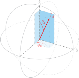
The CKM matrix V𝑉V requires 4 physical parameters, while the tree level SFCNC require 2, since r^[d]subscript^𝑟delimited-[]d\hat{r}_{{\rm[d]}} is a unit real vector. One can parametrise r^[d]subscript^𝑟delimited-[]d\hat{r}_{{\rm[d]}} in terms of two angles θdsubscript𝜃𝑑\theta_{d}, φdsubscript𝜑𝑑\varphi_{d}:

r^[d]=(sinθdcosφd,sinθdsinφd,cosθd),subscript^𝑟delimited-[]dsubscript𝜃𝑑subscript𝜑𝑑subscript𝜃𝑑subscript𝜑𝑑subscript𝜃𝑑\hat{r}_{{\rm[d]}}=(\sin\theta_{d}\cos\varphi_{d},\,\sin\theta_{d}\sin\varphi_{d},\,\cos\theta_{d})\,, (37)

as shown in Figure 1555The different products r^[d]ir^[d]jsubscript^𝑟delimited-[]d𝑖subscript^𝑟delimited-[]d𝑗\hat{r}_{{\rm[d]}i}\hat{r}_{{\rm[d]}j} controlling SFCNC are, simply, the areas of the shaded rectangular projections in the (i^,j^)^𝑖^𝑗(\hat{i},\hat{j}) planes in Figure 1..

Refer to caption
Figure 1: r^[d]subscript^𝑟delimited-[]d\hat{r}_{{\rm[d]}}.

The orthogonal matrix R𝑅R requires 3 real parameters; together with θ𝜃\theta and r^[d]subscript^𝑟delimited-[]d\hat{r}_{{\rm[d]}}, these 6 parameters match the parameters necessary to describe V𝑉V (4 parameters) and the products r^[d]jr^[d]ksubscript^𝑟delimited-[]d𝑗subscript^𝑟delimited-[]d𝑘\hat{r}_{{\rm[d]}j}\hat{r}_{{\rm[d]}k}, r^[u]jr^[u]ksubscript^𝑟delimited-[]u𝑗subscript^𝑟delimited-[]u𝑘\hat{r}_{{\rm[u]}j}\hat{r}_{{\rm[u]}k} (2 parameters). However, in terms of 𝒪Lusuperscriptsubscript𝒪𝐿𝑢\mathcal{O}_{L}^{u} and 𝒪Ldsuperscriptsubscript𝒪𝐿𝑑\mathcal{O}_{L}^{d}, there are a priori 3+3 real parameters; together with θ𝜃\theta, 7 parameters in all. This apparent mismatch can be readily understood: a common redefinition

𝒪Ld(cosαsinα0sinαcosα0001)𝒪Ld,𝒪Lu(cosαsinα0sinαcosα0001)𝒪Lu,formulae-sequencemaps-tosuperscriptsubscript𝒪𝐿𝑑𝛼𝛼0𝛼𝛼0001superscriptsubscript𝒪𝐿𝑑maps-tosuperscriptsubscript𝒪𝐿𝑢𝛼𝛼0𝛼𝛼0001superscriptsubscript𝒪𝐿𝑢\mathcal{O}_{L}^{d}\mapsto\left(\begin{smallmatrix}\cos\alpha&\sin\alpha&0\\ -\sin\alpha&\cos\alpha&0\\ 0&0&1\end{smallmatrix}\right)\,\mathcal{O}_{L}^{d},\qquad\mathcal{O}_{L}^{u}\mapsto\left(\begin{smallmatrix}\cos\alpha&\sin\alpha&0\\ -\sin\alpha&\cos\alpha&0\\ 0&0&1\end{smallmatrix}\right)\,\mathcal{O}_{L}^{u}, (38)

leaves R𝑅R, r^[d]subscript^𝑟delimited-[]d\hat{r}_{{\rm[d]}}, r^[u]subscript^𝑟delimited-[]u\hat{r}_{{\rm[u]}} and V𝑉V unchanged, effectively removing one parameter from the 𝒪Lusuperscriptsubscript𝒪𝐿𝑢\mathcal{O}_{L}^{u}, 𝒪Ldsuperscriptsubscript𝒪𝐿𝑑\mathcal{O}_{L}^{d}, parameter count. Consequently, it is convenient to adopt a parametrisation of R𝑅R of the form

R=(1000cα3sα30sα3cα3)(cα20sα2010sα20cα2)(cα1sα10sα1cα10001)=(cα1cα2sα1cα2sα2sα1cα3cα1sα2sα3cα1cα3sα1sα2sα3cα2sα3sα1sα3cα1sα2cα3cα1sα3sα1sα2cα3cα2cα3),𝑅matrix1000subscript𝑐subscript𝛼3subscript𝑠subscript𝛼30subscript𝑠subscript𝛼3subscript𝑐subscript𝛼3matrixsubscript𝑐subscript𝛼20subscript𝑠subscript𝛼2010subscript𝑠subscript𝛼20subscript𝑐subscript𝛼2matrixsubscript𝑐subscript𝛼1subscript𝑠subscript𝛼10subscript𝑠subscript𝛼1subscript𝑐subscript𝛼10001matrixsubscript𝑐subscript𝛼1subscript𝑐subscript𝛼2subscript𝑠subscript𝛼1subscript𝑐subscript𝛼2subscript𝑠subscript𝛼2subscript𝑠subscript𝛼1subscript𝑐subscript𝛼3subscript𝑐subscript𝛼1subscript𝑠subscript𝛼2subscript𝑠subscript𝛼3subscript𝑐subscript𝛼1subscript𝑐subscript𝛼3subscript𝑠subscript𝛼1subscript𝑠subscript𝛼2subscript𝑠subscript𝛼3subscript𝑐subscript𝛼2subscript𝑠subscript𝛼3subscript𝑠subscript𝛼1subscript𝑠subscript𝛼3subscript𝑐subscript𝛼1subscript𝑠subscript𝛼2subscript𝑐subscript𝛼3subscript𝑐subscript𝛼1subscript𝑠subscript𝛼3subscript𝑠subscript𝛼1subscript𝑠subscript𝛼2subscript𝑐subscript𝛼3subscript𝑐subscript𝛼2subscript𝑐subscript𝛼3R=\begin{pmatrix}1&0&0\\ 0&c_{\alpha_{3}}&s_{\alpha_{3}}\\ 0&-s_{\alpha_{3}}&c_{\alpha_{3}}\end{pmatrix}\begin{pmatrix}c_{\alpha_{2}}&0&s_{\alpha_{2}}\\ 0&1&0\\ -s_{\alpha_{2}}&0&c_{\alpha_{2}}\end{pmatrix}\begin{pmatrix}c_{\alpha_{1}}&s_{\alpha_{1}}&0\\ -s_{\alpha_{1}}&c_{\alpha_{1}}&0\\ 0&0&1\end{pmatrix}\\ =\begin{pmatrix}c_{\alpha_{1}}c_{\alpha_{2}}&s_{\alpha_{1}}c_{\alpha_{2}}&s_{\alpha_{2}}\\ -s_{\alpha_{1}}c_{\alpha_{3}}-c_{\alpha_{1}}s_{\alpha_{2}}s_{\alpha_{3}}&c_{\alpha_{1}}c_{\alpha_{3}}-s_{\alpha_{1}}s_{\alpha_{2}}s_{\alpha_{3}}&c_{\alpha_{2}}s_{\alpha_{3}}\\ s_{\alpha_{1}}s_{\alpha_{3}}-c_{\alpha_{1}}s_{\alpha_{2}}c_{\alpha_{3}}&-c_{\alpha_{1}}s_{\alpha_{3}}-s_{\alpha_{1}}s_{\alpha_{2}}c_{\alpha_{3}}&c_{\alpha_{2}}c_{\alpha_{3}}\end{pmatrix}\,, (39)

and a parametrisation of 𝒪Ldsuperscriptsubscript𝒪𝐿𝑑\mathcal{O}_{L}^{d} of the form666The rows in eq. (40) are simply unit vectors in spherical coordinates at r=r^[d]𝑟subscript^𝑟delimited-[]d\vec{r}=\hat{r}_{{\rm[d]}}, while α𝛼\alpha, in eq. (40) as in eq. (38), produces an irrelevant rotation around r^[d]subscript^𝑟delimited-[]d\hat{r}_{{\rm[d]}}.

𝒪Ld=(cαsα0sαcα0001)(cθdcφdcθdsφdsθdsφdcφd0sθdcφdsθdsφdcθd),superscriptsubscript𝒪𝐿𝑑matrixsubscript𝑐𝛼subscript𝑠𝛼0subscript𝑠𝛼subscript𝑐𝛼0001matrixsubscript𝑐subscript𝜃𝑑subscript𝑐subscript𝜑𝑑subscript𝑐subscript𝜃𝑑subscript𝑠subscript𝜑𝑑subscript𝑠subscript𝜃𝑑subscript𝑠subscript𝜑𝑑subscript𝑐subscript𝜑𝑑0subscript𝑠subscript𝜃𝑑subscript𝑐subscript𝜑𝑑subscript𝑠subscript𝜃𝑑subscript𝑠subscript𝜑𝑑subscript𝑐subscript𝜃𝑑\mathcal{O}_{L}^{d}=\begin{pmatrix}c_{\alpha}&s_{\alpha}&0\\ -s_{\alpha}&c_{\alpha}&0\\ 0&0&1\end{pmatrix}\begin{pmatrix}c_{\theta_{d}}c_{\varphi_{d}}&c_{\theta_{d}}s_{\varphi_{d}}&-s_{\theta_{d}}\\ -s_{\varphi_{d}}&c_{\varphi_{d}}&0\\ s_{\theta_{d}}c_{\varphi_{d}}&s_{\theta_{d}}s_{\varphi_{d}}&c_{\theta_{d}}\end{pmatrix}, (40)

where r^[d]subscript^𝑟delimited-[]d\hat{r}_{{\rm[d]}} is readily identified in the third row and the redundant α𝛼\alpha, as in eq. (38), can be set to α=0𝛼0\alpha=0. One can then concentrate on {α1,α2,α3,θd,φd,θ}subscript𝛼1subscript𝛼2subscript𝛼3subscript𝜃𝑑subscript𝜑𝑑𝜃\{\alpha_{1},\alpha_{2},\alpha_{3},\theta_{d},\varphi_{d},\theta\} in order to reproduce a realistic CKM matrix.

3.2 SFCNC and CP Violation in CKM

In eqs. (29)–(30), tree level SFCNC are a priori present in both the up and the down quark sectors and controlled by n^[q]in^[q]j=r^[q]ir^[q]jsuperscriptsubscript^𝑛delimited-[]q𝑖superscriptsubscript^𝑛delimited-[]q𝑗absentsubscript^𝑟delimited-[]q𝑖subscript^𝑟delimited-[]q𝑗\hat{n}_{{\rm[q]}i}^{\ast}\hat{n}_{{\rm[q]}j}^{\phantom{\ast}}=\hat{r}_{{\rm[q]}i}\hat{r}_{{\rm[q]}j}. Therefore, if r^[q]subscript^𝑟delimited-[]q\hat{r}_{{\rm[q]}} has a vanishing component, SFCNC in that sector (q=u𝑞𝑢q=u or d𝑑d) do only appear in one type of transition (the one not involving that component). If r^[q]subscript^𝑟delimited-[]q\hat{r}_{{\rm[q]}} had two vanishing components (then the remaining one equals ±1plus-or-minus1\pm 1), there would not be SFCNC in that sector: interstingly, in this model, having no tree level SFCNC in one quark sector is incompatible with a CP violating CKM matrix. This can be readily checked by noticing that, in that case, in eq. (34), the matrix with entries Sijsubscript𝑆𝑖𝑗S_{ij} has only a non vanishing row (column), corresponding to the absence of tree level SFCNC in the up (down) sector, for which Sij=Rijsubscript𝑆𝑖𝑗subscript𝑅𝑖𝑗S_{ij}=R_{ij}. Then, with i1i2subscript𝑖1subscript𝑖2i_{1}\neq i_{2} and j1j2subscript𝑗1subscript𝑗2j_{1}\neq j_{2}, in eq. (36) all terms except two out of the last four automatically vanish, and those two terms appear with opposite sign, giving Im(Vi1j1Vi1j2Vi2j2Vi2j1)=0Imsuperscriptsubscript𝑉subscript𝑖1subscript𝑗1absentsuperscriptsubscript𝑉subscript𝑖1subscript𝑗2superscriptsubscript𝑉subscript𝑖2subscript𝑗2absentsuperscriptsubscript𝑉subscript𝑖2subscript𝑗10\text{Im}\left({V_{i_{1}j_{1}}^{\phantom{\ast}}}{V_{i_{1}j_{2}}^{\ast}}{V_{i_{2}j_{2}}^{\phantom{\ast}}}{V_{i_{2}j_{1}}^{\ast}}\right)=0. As illustrated below, in subsection 3.4, this implies that a lower bound on the size of the second largest component in r^[q]subscript^𝑟delimited-[]q\hat{r}_{{\rm[q]}} should exist, that is a lower bound on the intensity of some SFCNC in both quark sectors. Appendix A completes the discussion of the interplay in this model among flavour non-conservation and CP violation in the CKM matrix.

3.3 A simple example

As a simplified example of how a realistic CKM matrix can be obtained, consider a scenario with

r^[d]=(cosφd,sinφd, 0).subscript^𝑟delimited-[]dsubscript𝜑𝑑subscript𝜑𝑑 0\hat{r}_{{\rm[d]}}=(\cos\varphi_{d},\ \sin\varphi_{d},\ 0)\,. (41)

Then, for i1=j1=1subscript𝑖1subscript𝑗11i_{1}=j_{1}=1, i2=j2=2subscript𝑖2subscript𝑗22i_{2}=j_{2}=2, eq. (36) reduces to

Im(V11V12V22V21)=12(R11R21+R12R22)(R12R21R11R22)sin2φdsin2θ.Imsuperscriptsubscript𝑉11absentsuperscriptsubscript𝑉12superscriptsubscript𝑉22absentsuperscriptsubscript𝑉2112subscript𝑅11subscript𝑅21subscript𝑅12subscript𝑅22subscript𝑅12subscript𝑅21subscript𝑅11subscript𝑅222subscript𝜑𝑑2𝜃\text{Im}\left({V_{11}^{\phantom{\ast}}}{V_{12}^{\ast}}{V_{22}^{\phantom{\ast}}}{V_{21}^{\ast}}\right)=\frac{1}{2}(R_{11}R_{21}+R_{12}R_{22})(R_{12}R_{21}-R_{11}R_{22})\sin 2\varphi_{d}\,\sin 2\theta\,. (42)

Since the rows of R𝑅R form a complete orthonormal set of 3-vectors,

R11R21+R12R22=R13R23,R12R21R11R22=R33,formulae-sequencesubscript𝑅11subscript𝑅21subscript𝑅12subscript𝑅22subscript𝑅13subscript𝑅23subscript𝑅12subscript𝑅21subscript𝑅11subscript𝑅22subscript𝑅33R_{11}R_{21}+R_{12}R_{22}=-R_{13}R_{23},\qquad R_{12}R_{21}-R_{11}R_{22}=-R_{33}, (43)

and eq. (45) is further reduced to

Im(V11V12V22V21)=12R13R23R33sin2φdsin2θ.Imsuperscriptsubscript𝑉11absentsuperscriptsubscript𝑉12superscriptsubscript𝑉22absentsuperscriptsubscript𝑉2112subscript𝑅13subscript𝑅23subscript𝑅332subscript𝜑𝑑2𝜃\text{Im}\left({V_{11}^{\phantom{\ast}}}{V_{12}^{\ast}}{V_{22}^{\phantom{\ast}}}{V_{21}^{\ast}}\right)=\frac{1}{2}R_{13}R_{23}R_{33}\sin 2\varphi_{d}\,\sin 2\theta\,. (44)

With R𝑅R in eq. (39), eq. (42) gives

Im(V11V12V22V21)=18cosα2sin2α2sin2α3sin2φdsin2θ.Imsuperscriptsubscript𝑉11absentsuperscriptsubscript𝑉12superscriptsubscript𝑉22absentsuperscriptsubscript𝑉2118subscript𝛼22subscript𝛼22subscript𝛼32subscript𝜑𝑑2𝜃\text{Im}\left({V_{11}^{\phantom{\ast}}}{V_{12}^{\ast}}{V_{22}^{\phantom{\ast}}}{V_{21}^{\ast}}\right)=\frac{1}{8}\cos\alpha_{2}\,\sin 2\alpha_{2}\,\sin 2\alpha_{3}\,\sin 2\varphi_{d}\,\sin 2\theta\,. (45)

A complete example of this type which reproduces correctly the CKM matrix, is given by:

θ=π/8,𝜃𝜋8\theta=\pi/8, (46)
R=(17×10603.746×1031.536×1041+8.41×1040.0413.743×1030.0411+8.48×10⁴),𝑅matrix17superscript10603.746superscript1031.536superscript10418.41superscript1040.0413.743superscript1030.04118.48superscript104R=\begin{pmatrix}1-7\times 10^{-6}&0&-3.746\times 10^{-3}\\ -1.536\times 10^{-4}&-1+8.41\times 10^{-4}&-0.041\\ -3.743\times 10^{-3}&0.041&-1+8.48\times 10^{-4}\end{pmatrix}\,, (47)

and

𝒪Ld=(0010.95090.309600.30960.95090).superscriptsubscript𝒪𝐿𝑑matrix0010.95090.309600.30960.95090\mathcal{O}_{L}^{d}=\begin{pmatrix}0&0&-1\\ 0.9509&0.3096&0\\ 0.3096&-0.9509&0\end{pmatrix}\,. (48)

The parameters underlying eqs. (47)–(48) have the values

R::𝑅absent\displaystyle R: α1=0,α2=3.746×10³,α3=0.041π,formulae-sequencesubscript𝛼10formulae-sequencesubscript𝛼23.746superscript103subscript𝛼30.041𝜋\displaystyle\quad\alpha_{1}=0,\ \alpha_{2}=-3.746\times 10^{-3},\ \alpha_{3}=0.041-\pi,
𝒪Ld::superscriptsubscript𝒪𝐿𝑑absent\displaystyle\mathcal{O}_{L}^{d}: θd=π/2,φd=1.2561,α=0.formulae-sequencesubscript𝜃𝑑𝜋2formulae-sequencesubscript𝜑𝑑1.2561𝛼0\displaystyle\quad\theta_{d}=\pi/2,\ \varphi_{d}=-1.2561,\ \alpha=0\,. (49)

For R𝑅R, α1=0subscript𝛼10\alpha_{1}=0 has been chosen for simplicity, since in this scenario it does not enter eq. (45). With the previous values, one can easily check that

|Vus|=0.2253,|Vub|=3.75×10³,|Vcb|=0.041,Im(V11V12V22V21)=3.195×10⁵.formulae-sequencesuperscriptsubscript𝑉𝑢𝑠absent0.2253formulae-sequencesuperscriptsubscript𝑉𝑢𝑏absent3.75superscript103formulae-sequencesuperscriptsubscript𝑉𝑐𝑏absent0.041Imsuperscriptsubscript𝑉11absentsuperscriptsubscript𝑉12superscriptsubscript𝑉22absentsuperscriptsubscript𝑉213.195superscript105|{V_{us}^{\phantom{\ast}}}|=0.2253,\ |{V_{ub}^{\phantom{\ast}}}|=3.75\times 10^{-3},\ |{V_{cb}^{\phantom{\ast}}}|=0.041,\ \text{Im}\left({V_{11}^{\phantom{\ast}}}{V_{12}^{\ast}}{V_{22}^{\phantom{\ast}}}{V_{21}^{\ast}}\right)=3.195\times 10^{-5}\,. (50)

Concerning the discussion in subsection 3.2, this example shows that, although the complete absence of tree level FCNC in one sector is incompatible with a CP violating CKM matrix, this incompatibility does not extend to the case of tree level SFCNC circumscribed to only one type of transition (in this example, ds𝑑𝑠d\leftrightarrow s transitions).

3.4 General case

The previous example illustrates that the CKM matrix can be adequately reproduced even in a restricted scenario where one has less number of free parameters. For the general case one can explore with a simple numerical analysis the regions of parameter space where the CKM matrix is in agreement with data, that is moduli |Vij|superscriptsubscript𝑉𝑖𝑗absent|{V_{ij}^{\phantom{\ast}}}| in the first two rows and the phase γ𝛾\gamma agree with experimental results [22].
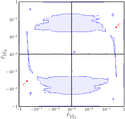
Figure 2(a) shows the region of the plane |sin2θ|2𝜃|\sin 2\theta| vs. θdsubscript𝜃𝑑\theta_{d} which can yield a good CKM matrix. It is to be noticed that (i) regions rather close to θ=0,π/2,π𝜃0𝜋2𝜋\theta=0,\pi/2,\pi, with |sin2θ|<1022𝜃superscript102|\sin 2\theta|<10^{-2}, are allowed and require θdπ/4,3π/4similar-tosubscript𝜃𝑑𝜋43𝜋4\theta_{d}\sim\pi/4,3\pi/4, while (ii) for |sin2θ|1similar-to2𝜃1|\sin 2\theta|\sim 1, allowed regions require θd0,π/2,πsimilar-tosubscript𝜃𝑑0𝜋2𝜋\theta_{d}\sim 0,\pi/2,\pi. In any case, sin2θ02𝜃0\sin 2\theta\neq 0 is a necessary requirement, as expected, since there is no CP violation in that limit.
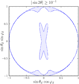
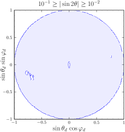
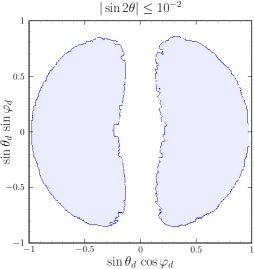
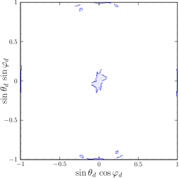
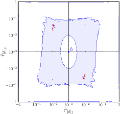
Figures 2(d)2(f) also show the allowed regions in the sinθdsinφdsubscript𝜃𝑑subscript𝜑𝑑\sin\theta_{d}\sin\varphi_{d} vs. sinθdcosφdsubscript𝜃𝑑subscript𝜑𝑑\sin\theta_{d}\cos\varphi_{d} plane777That is, the projection on the (1^,2^)^1^2(\hat{1},\hat{2}) plane of the allowed regions in the surface of the sphere of Figure 1., separating |sin2θ|1012𝜃superscript101|\sin 2\theta|\geq 10^{-1} in 2(d), 101|sin2θ|102superscript1012𝜃superscript10210^{-1}\geq|\sin 2\theta|\geq 10^{-2} in 2(e), and 102|sin2θ|superscript1022𝜃10^{-2}\geq|\sin 2\theta| in 2(f).
Following the discussion in subsection 3.2, one can sort the components of r^[d]subscript^𝑟delimited-[]d\hat{r}_{{\rm[d]}} according to their size:

|r^[d]Min||r^[d]Mid||r^[d]Max|.subscript^𝑟delimited-[]d𝑀𝑖𝑛subscript^𝑟delimited-[]d𝑀𝑖𝑑subscript^𝑟delimited-[]d𝑀𝑎𝑥|\hat{r}_{{\rm[d]}Min}|\leq|\hat{r}_{{\rm[d]}Mid}|\leq|\hat{r}_{{\rm[d]}Max}|\,. (51)

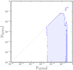
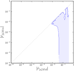
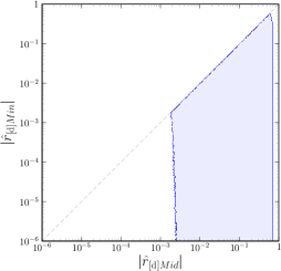
Incompatibility with a CP violating CKM matrix implies that |r^[d]Mid|0subscript^𝑟delimited-[]d𝑀𝑖𝑑0|\hat{r}_{{\rm[d]}Mid}|\neq 0, while the simple example in subsection 3.3 shows that |r^[d]Min|=0subscript^𝑟delimited-[]d𝑀𝑖𝑛0|\hat{r}_{{\rm[d]}Min}|=0 is allowed. Figure 2(b) shows the allowed region of |r^[d]Min|subscript^𝑟delimited-[]d𝑀𝑖𝑛|\hat{r}_{{\rm[d]}Min}| vs. |r^[d]Mid|subscript^𝑟delimited-[]d𝑀𝑖𝑑|\hat{r}_{{\rm[d]}Mid}| confirming that it is necessary that |r^[d]Mid|2×10³subscript^𝑟delimited-[]d𝑀𝑖𝑑2superscript103|\hat{r}_{{\rm[d]}Mid}|\geq 2\times 10^{-3}, while figure 2(c) corresponds similarly to r^[u]subscript^𝑟delimited-[]u\hat{r}_{{\rm[u]}}: both figures illustrate that, in this model, necessarily, there is at least some minimal presence of tree SFCNC888Notice that, consequently, θd=0,πsubscript𝜃𝑑0𝜋\theta_{d}=0,\pi are excluded: the resolution in Figures 2(a) and 2(d) is too coarse to observe that, while Figures 2(b) and 2(c) clearly illustrate the point..
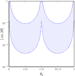
Refer to caption
(a) sin2θ2𝜃\sin 2\theta vs. θdsubscript𝜃𝑑\theta_{d}
Refer to caption
(b) |r^[d]Min|subscript^𝑟delimited-[]d𝑀𝑖𝑛|\hat{r}_{{\rm[d]}Min}| vs. |r^[d]Mid|subscript^𝑟delimited-[]d𝑀𝑖𝑑|\hat{r}_{{\rm[d]}Mid}|.
Refer to caption
(c) |r^[u]Min|subscript^𝑟delimited-[]u𝑀𝑖𝑛|\hat{r}_{{\rm[u]}Min}| vs. |r^[u]Mid|subscript^𝑟delimited-[]u𝑀𝑖𝑑|\hat{r}_{{\rm[u]}Mid}|.
Refer to caption
(d)
Refer to caption
(e)
Refer to caption
(f)
Figure 2: Regions (at 99% C.L.) which reproduce a realistic CKM matrix are shown.

In conclusion, it is clear that the first requirement on the model, i.e. that it can reproduce the observed CKM matrix, can be fulfilled.

4 The scalar potential with real couplings

We consider the 2HDM with CP invariance and impose the 2subscript2\mathbb{Z}_{2} symmetry of eq. (2) which is only softly broken by a μ12subscript𝜇12\mu_{12} term. All couplings are real, so that CP holds at the Lagrangian level. The scalar potential can be written:

𝒱(Φ1,Φ2)=μ112Φ1Φ1+μ222Φ2Φ2+μ122(Φ1Φ2+Φ2Φ1)+λ1(Φ1Φ1)2+λ2(Φ2Φ2)2+2λ3(Φ1Φ1)(Φ2Φ2)+2λ4(Φ1Φ2)(Φ2Φ1)+λ5[(Φ1Φ2)2+(Φ2Φ1)2].𝒱superscriptsubscriptΦ1absentsuperscriptsubscriptΦ2absentsuperscriptsubscript𝜇112superscriptsubscriptΦ1superscriptsubscriptΦ1absentsuperscriptsubscript𝜇222superscriptsubscriptΦ2superscriptsubscriptΦ2absentsuperscriptsubscript𝜇122superscriptsubscriptΦ1superscriptsubscriptΦ2absentsuperscriptsubscriptΦ2superscriptsubscriptΦ1absentsubscript𝜆1superscriptsuperscriptsubscriptΦ1superscriptsubscriptΦ1absent2subscript𝜆2superscriptsuperscriptsubscriptΦ2superscriptsubscriptΦ2absent22subscript𝜆3superscriptsubscriptΦ1superscriptsubscriptΦ1absentsuperscriptsubscriptΦ2superscriptsubscriptΦ2absent2subscript𝜆4superscriptsubscriptΦ1superscriptsubscriptΦ2absentsuperscriptsubscriptΦ2superscriptsubscriptΦ1absentsubscript𝜆5delimited-[]superscriptsuperscriptsubscriptΦ1superscriptsubscriptΦ2absent2superscriptsuperscriptsubscriptΦ2superscriptsubscriptΦ1absent2\mathscr{V}(\Phi_{1}^{\phantom{\dagger}},\Phi_{2}^{\phantom{\dagger}})=\mu_{11}^{2}\Phi_{1}^{\dagger}\Phi_{1}^{\phantom{\dagger}}+\mu_{22}^{2}\Phi_{2}^{\dagger}\Phi_{2}^{\phantom{\dagger}}+\mu_{12}^{2}(\Phi_{1}^{\dagger}\Phi_{2}^{\phantom{\dagger}}+\Phi_{2}^{\dagger}\Phi_{1}^{\phantom{\dagger}})+\lambda_{1}(\Phi_{1}^{\dagger}\Phi_{1}^{\phantom{\dagger}})^{2}+\lambda_{2}(\Phi_{2}^{\dagger}\Phi_{2}^{\phantom{\dagger}})^{2}\\ +2\lambda_{3}(\Phi_{1}^{\dagger}\Phi_{1}^{\phantom{\dagger}})(\Phi_{2}^{\dagger}\Phi_{2}^{\phantom{\dagger}})+2\lambda_{4}(\Phi_{1}^{\dagger}\Phi_{2}^{\phantom{\dagger}})(\Phi_{2}^{\dagger}\Phi_{1}^{\phantom{\dagger}})+\lambda_{5}[(\Phi_{1}^{\dagger}\Phi_{2}^{\phantom{\dagger}})^{2}+(\Phi_{2}^{\dagger}\Phi_{1}^{\phantom{\dagger}})^{2}]\,. (52)

The vacuum expectation values are

Φ1=(0eiθ1v1/2),Φ2=(0eiθ2v2/2),formulae-sequencedelimited-⟨⟩superscriptsubscriptΦ1absentmatrix0superscript𝑒𝑖subscript𝜃1subscript𝑣12delimited-⟨⟩superscriptsubscriptΦ2absentmatrix0superscript𝑒𝑖subscript𝜃2subscript𝑣22\langle\Phi_{1}^{\phantom{\dagger}}\rangle=\begin{pmatrix}0\\ e^{i\theta_{1}}v_{1}/\sqrt{2}\end{pmatrix},\quad\langle\Phi_{2}^{\phantom{\dagger}}\rangle=\begin{pmatrix}0\\ e^{i\theta_{2}}v_{2}/\sqrt{2}\end{pmatrix}, (53)

and break electroweak symmetry spontaneously. As anticipated in section 2, we use θ=θ2θ1𝜃subscript𝜃2subscript𝜃1\theta=\theta_{2}-\theta_{1}, v2=v12+v22superscript𝑣2superscriptsubscript𝑣12superscriptsubscript𝑣22v^{2}=v_{1}^{2}+v_{2}^{2}, cβ=cosβv1/vsubscript𝑐𝛽𝛽subscript𝑣1𝑣c_{\beta}=\cos\beta\equiv v_{1}/v, sβ=sinβv2/vsubscript𝑠𝛽𝛽subscript𝑣2𝑣s_{\beta}=\sin\beta\equiv v_{2}/v and tβtanβsubscript𝑡𝛽𝛽t_{\beta}\equiv\tan\beta, with v10subscript𝑣10v_{1}\geq 0, v20subscript𝑣20v_{2}\geq 0.

4.1 Minimization

The minimization conditions for V(v1,v2,θ)𝒱(Φ1,Φ2)𝑉subscript𝑣1subscript𝑣2𝜃𝒱delimited-⟨⟩superscriptsubscriptΦ1absentdelimited-⟨⟩superscriptsubscriptΦ2absentV(v_{1},v_{2},\theta)\equiv\mathscr{V}(\langle\Phi_{1}^{\phantom{\dagger}}\rangle,\langle\Phi_{2}^{\phantom{\dagger}}\rangle) are

Vθ=v1v2sinθ(μ122+2λ5v1v2cosθ)=0,𝑉𝜃subscript𝑣1subscript𝑣2𝜃superscriptsubscript𝜇1222subscript𝜆5subscript𝑣1subscript𝑣2𝜃0\displaystyle\frac{\partial V}{\partial\theta}=-v_{1}v_{2}\sin\theta(\mu_{12}^{2}+2\lambda_{5}v_{1}v_{2}\cos\theta)=0, (54)
Vv1=μ112v1+λ1v13+(λ3+λ4)v1v22+v2(μ122cosθ+λ5v1v2cos2θ)=0,𝑉subscript𝑣1superscriptsubscript𝜇112subscript𝑣1subscript𝜆1superscriptsubscript𝑣13subscript𝜆3subscript𝜆4subscript𝑣1superscriptsubscript𝑣22subscript𝑣2superscriptsubscript𝜇122𝜃subscript𝜆5subscript𝑣1subscript𝑣22𝜃0\displaystyle\frac{\partial V}{\partial v_{1}}=\mu_{11}^{2}v_{1}+\lambda_{1}v_{1}^{3}+(\lambda_{3}+\lambda_{4})v_{1}v_{2}^{2}+v_{2}(\mu_{12}^{2}\cos\theta+\lambda_{5}v_{1}v_{2}\cos 2\theta)=0, (55)
Vv2=μ222v2+λ2v23+(λ3+λ4)v12v2+v1(μ122cosθ+λ5v1v2cos2θ)=0.𝑉subscript𝑣2superscriptsubscript𝜇222subscript𝑣2subscript𝜆2superscriptsubscript𝑣23subscript𝜆3subscript𝜆4superscriptsubscript𝑣12subscript𝑣2subscript𝑣1superscriptsubscript𝜇122𝜃subscript𝜆5subscript𝑣1subscript𝑣22𝜃0\displaystyle\frac{\partial V}{\partial v_{2}}=\mu_{22}^{2}v_{2}+\lambda_{2}v_{2}^{3}+(\lambda_{3}+\lambda_{4})v_{1}^{2}v_{2}+v_{1}(\mu_{12}^{2}\cos\theta+\lambda_{5}v_{1}v_{2}\cos 2\theta)=0. (56)

In order to have spontaneous CP violation, we consider a solution {v1,v2,θ}subscript𝑣1subscript𝑣2𝜃\{v_{1},v_{2},\theta\} of eqs. (54)–(56) with θ0,±π/2,±π𝜃0plus-or-minus𝜋2plus-or-minus𝜋\theta\neq 0,\pm\pi/2,\pm\pi. From eq. (54) one obtains

cosθ=μ1222λ5v1v2.𝜃superscriptsubscript𝜇1222subscript𝜆5subscript𝑣1subscript𝑣2\cos\theta=\frac{-\mu_{12}^{2}}{2\lambda_{5}v_{1}v_{2}}\,. (57)

Notice that, in addition to θ𝜃\theta, θ𝜃-\theta is also a solution. It is obvious that for θ=0,π𝜃0𝜋\theta=0,\pi the vacuum is CP invariant. It has also been shown [13] that for θ=π/2𝜃𝜋2\theta=\pi/2 the vacuum is also CP invariant. Note from eq. (57) that θ=±π/2𝜃plus-or-minus𝜋2\theta=\pm\pi/2 is obtained when μ122=0superscriptsubscript𝜇1220\mu_{12}^{2}=0. In this case, the scalar potential is invariant under the 2subscript2\mathbb{Z}_{2} symmetry of eq. (2). This symmetry allows the two scalar fields Φ1superscriptsubscriptΦ1absent\Phi_{1}^{\phantom{\dagger}}, Φ2superscriptsubscriptΦ2absent\Phi_{2}^{\phantom{\dagger}} to have either equal or opposite CP parities. It is this freedom that is used to construct a simple proof [13] that for θ=±π/2𝜃plus-or-minus𝜋2\theta=\pm\pi/2, the vacuum is CP invariant.
One can trade μ112superscriptsubscript𝜇112\mu_{11}^{2}, μ222superscriptsubscript𝜇222\mu_{22}^{2} and μ122superscriptsubscript𝜇122\mu_{12}^{2} for other parameters using eqs. (54)–(56):

μ122=2λ5v1v2cosθ,superscriptsubscript𝜇1222subscript𝜆5subscript𝑣1subscript𝑣2𝜃\displaystyle\mu_{12}^{2}=-2\lambda_{5}v_{1}v_{2}\cos\theta, (58)
μ112=(λ1v12+(λ3+λ4λ5)v22),superscriptsubscript𝜇112subscript𝜆1superscriptsubscript𝑣12subscript𝜆3subscript𝜆4subscript𝜆5superscriptsubscript𝑣22\displaystyle\mu_{11}^{2}=-(\lambda_{1}v_{1}^{2}+(\lambda_{3}+\lambda_{4}-\lambda_{5})v_{2}^{2}), (59)
μ222=(λ2v22+(λ3+λ4λ5)v12).superscriptsubscript𝜇222subscript𝜆2superscriptsubscript𝑣22subscript𝜆3subscript𝜆4subscript𝜆5superscriptsubscript𝑣12\displaystyle\mu_{22}^{2}=-(\lambda_{2}v_{2}^{2}+(\lambda_{3}+\lambda_{4}-\lambda_{5})v_{1}^{2}). (60)

That is, imposing eqs. (58)–(60) on 𝒱(Φ1,Φ2)𝒱superscriptsubscriptΦ1absentsuperscriptsubscriptΦ2absent\mathscr{V}(\Phi_{1}^{\phantom{\dagger}},\Phi_{2}^{\phantom{\dagger}}) in eq. (52), one is selecting a scalar potential where, at least, the necessary minimization conditions in eqs. (54)–(56) are satisfied for generic {v1,v2,θ}subscript𝑣1subscript𝑣2𝜃\{v_{1},v_{2},\theta\}. One can in addition choose v12+v22=v2=(246 GeV)2superscriptsubscript𝑣12superscriptsubscript𝑣22superscript𝑣2superscript246 GeV2v_{1}^{2}+v_{2}^{2}=v^{2}=(246\text{ GeV})^{2} for appropriate electroweak symmetry breaking without loss of generality (this is enforced, for example, by a simple rescaling of the parameters in the potential). Fixing v2superscript𝑣2v^{2} in that manner, one is left with a candidate minimum characterised by the values of θ𝜃\theta and tanβ=v2/v1𝛽subscript𝑣2subscript𝑣1\tan\beta=v_{2}/v_{1}, which remain free parameters that we can choose at will, up to the different constraints on the scalar potential to be discussed later:

  1. 1.

    the potential is bounded from below and V(v1,v2,θ)𝑉subscript𝑣1subscript𝑣2𝜃V(v_{1},v_{2},\theta) is the lowest lying minimum;

  2. 2.

    perturbative unitarity bounds on scattering processes in the scalar sector are respected.

Expanding ΦjsuperscriptsubscriptΦ𝑗absent\Phi_{j}^{\phantom{\dagger}} around the candidate vacuum in eq. (53)

Φj=eiθj(φj+12(vj+ρj+iηj)),superscriptsubscriptΦ𝑗absentsuperscript𝑒𝑖subscript𝜃𝑗matrixsubscriptsuperscript𝜑𝑗12subscript𝑣𝑗subscript𝜌𝑗𝑖subscript𝜂𝑗\Phi_{j}^{\phantom{\dagger}}=e^{i\theta_{j}}\begin{pmatrix}\varphi^{+}_{j}\\ \frac{1}{\sqrt{2}}(v_{j}+\rho_{j}+i\eta_{j})\end{pmatrix}\,, (61)

we can now explore the different mass terms for the charged and neutral scalars. Requiring that the mass parameters of all the physical scalars are positive ensures, at least, that the candidate minimum is a local minimum of the potential. In the Higgs basis of eq. (5), the expansion of the fields reads

H1=(G+(v+H0+iG0)/2),H2=(H+(R0+iI0)/2),formulae-sequencesubscript𝐻1matrixsuperscript𝐺𝑣superscript𝐻0𝑖superscript𝐺02subscript𝐻2matrixsuperscriptHsuperscript𝑅0𝑖superscript𝐼02H_{1}=\begin{pmatrix}G^{+}\\ (v+{H}^{0}+iG^{0})/\sqrt{2}\end{pmatrix},\quad H_{2}=\begin{pmatrix}{\rm H}^{+}\\ ({R}^{0}+i{I}^{0})/\sqrt{2}\end{pmatrix}, (62)
(G+H+)=β(φ1+φ2+),(G0I0)=β(η1η2),(H0R0)=β(ρ1ρ2),formulae-sequencematrixsuperscript𝐺superscriptHsuperscriptsubscript𝛽absentmatrixsuperscriptsubscript𝜑1superscriptsubscript𝜑2formulae-sequencematrixsuperscript𝐺0superscript𝐼0superscriptsubscript𝛽absentmatrixsubscript𝜂1subscript𝜂2matrixsuperscript𝐻0superscript𝑅0superscriptsubscript𝛽absentmatrixsubscript𝜌1subscript𝜌2\begin{pmatrix}G^{+}\\ {\rm H}^{+}\end{pmatrix}=\mathcal{R}_{\beta}^{\phantom{T}}\begin{pmatrix}\varphi_{1}^{+}\\ \varphi_{2}^{+}\end{pmatrix},\ \begin{pmatrix}G^{0}\\ {I}^{0}\end{pmatrix}=\mathcal{R}_{\beta}^{\phantom{T}}\begin{pmatrix}\eta_{1}\\ \eta_{2}\end{pmatrix},\ \begin{pmatrix}{H}^{0}\\ {R}^{0}\end{pmatrix}=\mathcal{R}_{\beta}^{\phantom{T}}\begin{pmatrix}\rho_{1}\\ \rho_{2}\end{pmatrix}, (63)

with the would-be Goldstone bosons G±superscript𝐺plus-or-minusG^{\pm} and G0superscript𝐺0G^{0} readily identified

G±=cβφ1±sβφ2±,G0=cβη1sβη2.formulae-sequencesuperscript𝐺plus-or-minussubscript𝑐𝛽superscriptsubscript𝜑1plus-or-minussubscript𝑠𝛽superscriptsubscript𝜑2plus-or-minussuperscript𝐺0subscript𝑐𝛽subscript𝜂1subscript𝑠𝛽subscript𝜂2G^{\pm}=c_{\beta}\varphi_{1}^{\pm}-s_{\beta}\varphi_{2}^{\pm},\quad G^{0}=c_{\beta}\eta_{1}-s_{\beta}\eta_{2}\,. (64)

4.2 Scalar masses and mixings

4.2.1 Charged scalar

The transformation into the Higgs basis also gives the mass term of the charged scalar H±=sβφ1±cβφ2±superscriptHplus-or-minussubscript𝑠𝛽superscriptsubscript𝜑1plus-or-minussubscript𝑐𝛽superscriptsubscript𝜑2plus-or-minus{\rm H}^{\pm}=s_{\beta}\varphi_{1}^{\pm}-c_{\beta}\varphi_{2}^{\pm},

𝒱(Φ1,Φ2)v2(λ5λ4)H+HmH±2=v2(λ5λ4).superset-of𝒱superscriptsubscriptΦ1absentsuperscriptsubscriptΦ2absentsuperscript𝑣2subscript𝜆5subscript𝜆4superscriptHsuperscriptHsuperscriptsubscript𝑚superscriptHplus-or-minus2superscript𝑣2subscript𝜆5subscript𝜆4\mathscr{V}(\Phi_{1}^{\phantom{\dagger}},\Phi_{2}^{\phantom{\dagger}})\ \supset\ v^{2}(\lambda_{5}-\lambda_{4}){\rm H}^{+}{\rm H}^{-}\,\Rightarrow m_{{\rm H}^{\pm}}^{2}=v^{2}(\lambda_{5}-\lambda_{4})\,. (65)

Notice that, in order to choose a set of independent parameters, eq. (65) will allow us to trade λ4subscript𝜆4\lambda_{4} for mH±2superscriptsubscript𝑚superscriptHplus-or-minus2m_{{\rm H}^{\pm}}^{2} and λ5subscript𝜆5\lambda_{5}. Furthermore, since λ5subscript𝜆5\lambda_{5} and λ4subscript𝜆4\lambda_{4} are subject to the constraints on the scalar potential discussed in appendix B, mH±subscript𝑚superscriptHplus-or-minusm_{{\rm H}^{\pm}} has a limited allowed range: for example, if λ5λ4<20subscript𝜆5subscript𝜆420\lambda_{5}-\lambda_{4}<20, then it follows that mH±<9mhsubscript𝑚superscriptHplus-or-minus9subscript𝑚hm_{{\rm H}^{\pm}}<9m_{{\rm h}}.

4.2.2 Neutral scalars

For the neutral scalar sector, the mass terms are

𝒱(Φ1,Φ2)12(H0R0I0)02(H0R0I0),12matrixsuperscript𝐻0superscript𝑅0superscript𝐼0superscriptsubscript02matrixsuperscript𝐻0superscript𝑅0superscript𝐼0𝒱superscriptsubscriptΦ1absentsuperscriptsubscriptΦ2absent\mathscr{V}(\Phi_{1}^{\phantom{\dagger}},\Phi_{2}^{\phantom{\dagger}})\ \supset\ \frac{1}{2}\begin{pmatrix}{H}^{0}&{R}^{0}&{I}^{0}\end{pmatrix}\ \mathcal{M}_{0}^{2}\ \begin{pmatrix}{H}^{0}\\ {R}^{0}\\ {I}^{0}\end{pmatrix}\,, (66)

with 02=02Tsuperscriptsubscript02superscriptsuperscriptsubscript02𝑇\mathcal{M}_{0}^{2}={\mathcal{M}_{0}^{2}}^{T}, and

[02]11=2v2{λ1cβ4+λ2sβ4+2cβ2sβ2[λ345+2λ5cθ2]},subscriptdelimited-[]superscriptsubscript02112superscript𝑣2subscript𝜆1superscriptsubscript𝑐𝛽4subscript𝜆2superscriptsubscript𝑠𝛽42superscriptsubscript𝑐𝛽2superscriptsubscript𝑠𝛽2delimited-[]subscript𝜆3452subscript𝜆5superscriptsubscript𝑐𝜃2\displaystyle[\mathcal{M}_{0}^{2}]_{11}=2v^{2}\left\{\lambda_{1}c_{\beta}^{4}+\lambda_{2}s_{\beta}^{4}+2c_{\beta}^{2}s_{\beta}^{2}[\lambda_{345}+2\lambda_{5}c_{\theta}^{2}]\right\},
[02]22=2v2{cβ2sβ2(λ1+λ22λ345)+λ5(cβ2sβ2)2cθ2},subscriptdelimited-[]superscriptsubscript02222superscript𝑣2superscriptsubscript𝑐𝛽2superscriptsubscript𝑠𝛽2subscript𝜆1subscript𝜆22subscript𝜆345subscript𝜆5superscriptsuperscriptsubscript𝑐𝛽2superscriptsubscript𝑠𝛽22superscriptsubscript𝑐𝜃2\displaystyle[\mathcal{M}_{0}^{2}]_{22}=2v^{2}\left\{c_{\beta}^{2}s_{\beta}^{2}(\lambda_{1}+\lambda_{2}-2\lambda_{345})+\lambda_{5}(c_{\beta}^{2}-s_{\beta}^{2})^{2}c_{\theta}^{2}\right\},
[02]12=2v2sβcβ{λ1cβ2+λ2sβ2+(cβ2sβ2)[λ345+2λ5cθ2])},\displaystyle[\mathcal{M}_{0}^{2}]_{12}=2v^{2}s_{\beta}c_{\beta}\left\{-\lambda_{1}c_{\beta}^{2}+\lambda_{2}s_{\beta}^{2}+(c_{\beta}^{2}-s_{\beta}^{2})[\lambda_{345}+2\lambda_{5}c_{\theta}^{2}])\right\},
[02]13=v2λ5s2βs2θ,subscriptdelimited-[]superscriptsubscript0213superscript𝑣2subscript𝜆5subscript𝑠2𝛽subscript𝑠2𝜃\displaystyle[\mathcal{M}_{0}^{2}]_{13}=-v^{2}\lambda_{5}s_{2\beta}s_{2\theta},
[02]23=v2λ5c2βs2θ,subscriptdelimited-[]superscriptsubscript0223superscript𝑣2subscript𝜆5subscript𝑐2𝛽subscript𝑠2𝜃\displaystyle[\mathcal{M}_{0}^{2}]_{23}=-v^{2}\lambda_{5}c_{2\beta}s_{2\theta},
[02]33=2v2λ5sθ2,subscriptdelimited-[]superscriptsubscript02332superscript𝑣2subscript𝜆5superscriptsubscript𝑠𝜃2\displaystyle[\mathcal{M}_{0}^{2}]_{33}=2v^{2}\lambda_{5}s_{\theta}^{2}, (67)

with, we recall, the shorthand notation cx=cosxsubscript𝑐𝑥𝑥c_{x}=\cos x, sx=sinxsubscript𝑠𝑥𝑥s_{x}=\sin x, and λ345λ3+λ4λ5subscript𝜆345subscript𝜆3subscript𝜆4subscript𝜆5\lambda_{345}\equiv\lambda_{3}+\lambda_{4}-\lambda_{5}.
For λ5s2θ0subscript𝜆5subscript𝑠2𝜃0\lambda_{5}s_{2\theta}\neq 0, attending to [02]130subscriptdelimited-[]superscriptsubscript02130[\mathcal{M}_{0}^{2}]_{13}\neq 0 and [02]230subscriptdelimited-[]superscriptsubscript02230[\mathcal{M}_{0}^{2}]_{23}\neq 0 above, there is scalar-pseudoscalar mixing, as it is expected from spontaneous breaking of CP in the scalar sector. 02superscriptsubscript02\mathcal{M}_{0}^{2} is diagonalised through a real orthogonal transformation \mathcal{R}

T02=diag(mh2,mH2,mA2),1=T.formulae-sequencesuperscript𝑇superscriptsubscript02diagsuperscriptsubscript𝑚h2superscriptsubscript𝑚H2superscriptsubscript𝑚A2superscript1superscript𝑇\mathcal{R}^{T}\,\mathcal{M}_{0}^{2}\,\mathcal{R}=\text{diag}(m_{{\rm h}}^{2},m_{{\rm H}}^{2},m_{{\rm A}}^{2})\,,\quad\mathcal{R}^{-1}=\mathcal{R}^{T}. (68)

The physical neutral scalars are

(hHA)=T(H0R0I0),matrixhHAsuperscript𝑇matrixsuperscript𝐻0superscript𝑅0superscript𝐼0\begin{pmatrix}{\rm h}\\ {\rm H}\\ {\rm A}\end{pmatrix}=\mathcal{R}^{T}\begin{pmatrix}{H}^{0}\\ {R}^{0}\\ {I}^{0}\end{pmatrix}\,, (69)

and we assume hh{\rm h} to be the lightest one, the Higgs-like neutral scalar with mh=125subscript𝑚h125m_{{\rm h}}=125 GeV. With 02superscriptsubscript02\mathcal{M}_{0}^{2} in eqs. (67), \mathcal{R} “mixes”, a priori, all three neutral scalars. It is interesting to notice that

Tr[02]=mh2+mH2+mA2=2v2[λ1cβ2+λ2sβ2+λ5],Trdelimited-[]superscriptsubscript02superscriptsubscript𝑚h2superscriptsubscript𝑚H2superscriptsubscript𝑚A22superscript𝑣2delimited-[]subscript𝜆1superscriptsubscript𝑐𝛽2subscript𝜆2superscriptsubscript𝑠𝛽2subscript𝜆5\text{Tr}[\mathcal{M}_{0}^{2}]=m_{{\rm h}}^{2}+m_{{\rm H}}^{2}+m_{{\rm A}}^{2}=2v^{2}[\lambda_{1}c_{\beta}^{2}+\lambda_{2}s_{\beta}^{2}+\lambda_{5}]\,, (70)

and

det[02]=mh2mH2mA2=2v6λ5(λ1λ2λ3452)sin22βsin2θ.delimited-[]superscriptsubscript02superscriptsubscript𝑚h2superscriptsubscript𝑚H2superscriptsubscript𝑚A22superscript𝑣6subscript𝜆5subscript𝜆1subscript𝜆2superscriptsubscript𝜆3452superscript22𝛽superscript2𝜃\det[\mathcal{M}_{0}^{2}]=m_{{\rm h}}^{2}\,m_{{\rm H}}^{2}\,m_{{\rm A}}^{2}=2v^{6}\lambda_{5}(\lambda_{1}\lambda_{2}-\lambda_{345}^{2})\sin^{2}2\beta\,\sin^{2}\theta\,. (71)

As explained in appendix B, since it is necessary that λ5>0subscript𝜆50\lambda_{5}>0, it is also required that λ1λ2>λ3452subscript𝜆1subscript𝜆2superscriptsubscript𝜆3452\lambda_{1}\lambda_{2}>\lambda_{345}^{2} for V(v1,v2,θ)𝑉subscript𝑣1subscript𝑣2𝜃V(v_{1},v_{2},\theta) to be, at least, a local minimum (for which, necessarily, det[02]>0delimited-[]superscriptsubscript020\det[\mathcal{M}_{0}^{2}]>0).
Equations (70) and (71) encode in a transparent manner several interesting properties of the model. First, since the different λjsubscript𝜆𝑗\lambda_{j} are bounded by the requirements discussed in appendix B (in particular by perturbative unitarity), and sin22β1superscript22𝛽1\sin^{2}2\beta\leq 1 and sin2θ1superscript2𝜃1\sin^{2}\theta\leq 1, the masses of the new scalars HH{\rm H}, AA{\rm A}, H±superscriptHplus-or-minus{\rm H}^{\pm}, have a limited allowed range. For a very crude estimate, consider for example λ1cβ2+λ2sβ2+λ510similar-tosubscript𝜆1superscriptsubscript𝑐𝛽2subscript𝜆2superscriptsubscript𝑠𝛽2subscript𝜆510\lambda_{1}c_{\beta}^{2}+\lambda_{2}s_{\beta}^{2}+\lambda_{5}\sim 10 in eq. (70): with v2mhsimilar-to-or-equals𝑣2subscript𝑚hv\simeq 2m_{{\rm h}}, mH2+mA280mh2similar-tosuperscriptsubscript𝑚H2superscriptsubscript𝑚A280superscriptsubscript𝑚h2m_{{\rm H}}^{2}+m_{{\rm A}}^{2}\sim 80m_{{\rm h}}^{2} and it is clear that the smaller among mHsubscript𝑚Hm_{{\rm H}} and mAsubscript𝑚Am_{{\rm A}} cannot be larger than 6mhsimilar-toabsent6subscript𝑚h\sim 6m_{{\rm h}}, while the larger among mHsubscript𝑚Hm_{{\rm H}} and mAsubscript𝑚Am_{{\rm A}} cannot be larger than 9mhsimilar-toabsent9subscript𝑚h\sim 9m_{{\rm h}}.
On the other hand, from eq. (71), for sin2β1much-less-than2𝛽1\sin 2\beta\ll 1, at least one neutral scalar should be light and either tanβ1much-greater-than𝛽1\tan\beta\gg 1 or tan1β1much-greater-thansuperscript1𝛽1\tan^{-1}\beta\gg 1, which enhance SFCNC couplings. One can than expect that sin2β1much-less-than2𝛽1\sin 2\beta\ll 1 will be disfavoured by the constraints discussed in section 6, while tanβtan1β1similar-to𝛽superscript1𝛽similar-to1\tan\beta\sim\tan^{-1}\beta\sim 1 are easier to accommodate. Finally, it is to be noticed that for sinθ=1𝜃1\sin\theta=1, there is no mixing among {h,H}hH\{{\rm h},{\rm H}\} and AA{\rm A} (and mA2=2λ5v2superscriptsubscript𝑚A22subscript𝜆5superscript𝑣2m_{{\rm A}}^{2}=2\lambda_{5}v^{2}), and, as discussed, no spontaneous CP violation and a real CKM matrix. For sinθ=0𝜃0\sin\theta=0, mA=0subscript𝑚A0m_{{\rm A}}=0 and thus for |sinθ|1much-less-than𝜃1|\sin\theta|\ll 1, one could expect again the presence of at least one light scalar.
From the previous comments, it emerges that in this model there is limited room to have a scalar sector where (i) hh{\rm h} is a Higgs boson with quite SM-like properties and (ii) mH±subscript𝑚superscriptHplus-or-minusm_{{\rm H}^{\pm}}, mHsubscript𝑚Hm_{{\rm H}}, mAmhmuch-greater-thansubscript𝑚Asubscript𝑚hm_{{\rm A}}\gg m_{{\rm h}}. In this model, there is no decoupling regime for the new scalars. It is also clear, with these values, that the new scalars should be produced at the LHC. Nevertheless, the most relevant production and decay modes for their discovery will vary significantly between different regions of parameter space, including the Yukawa couplings discussed in section 5, and also the details of the lepton sector, and are thus beyond the scope of this work.

4.3 A simple analysis of the scalar sector

As a first step in the direction of the complete analysis of section 6, in this subsection we analyse the available parameter space of the scalar sector of the model, considering the following constraints.

  • Agreement with electroweak precision data, in particular the oblique parameters S𝑆S and T𝑇T [23].

  • Boundedness of the scalar potential and perturbative unitarity of the scattering processes, controlled by the scalar quartic couplings λjsubscript𝜆𝑗\lambda_{j}, as described, respectively, in appendices B.2 and B.3.

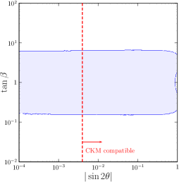
  • We only consider mH±subscript𝑚superscriptHplus-or-minusm_{{\rm H}^{\pm}}, mHsubscript𝑚Hm_{{\rm H}}, mA150subscript𝑚A150m_{{\rm A}}\geq 150 GeV; although masses of new scalars below 150150150 GeV are not automatically excluded by existing constraints, they would require specific analyses, interesting on their own, which are out of the scope of the present work. Furthermore, attending to eq. (71) and the related discussion, imposing this requirement on mHsubscript𝑚Hm_{{\rm H}} and mAsubscript𝑚Am_{{\rm A}} translates into a lower bound on s2β2superscriptsubscript𝑠2𝛽2s_{2\beta}^{2} and sθ2superscriptsubscript𝑠𝜃2s_{\theta}^{2}. For a simple estimate one can take λ5(λ1λ2λ3452)<102subscript𝜆5subscript𝜆1subscript𝜆2superscriptsubscript𝜆3452superscript102\lambda_{5}(\lambda_{1}\lambda_{2}-\lambda_{345}^{2})<10^{2}, which gives (for mHsubscript𝑚Hm_{{\rm H}}, mA150subscript𝑚A150m_{{\rm A}}\geq 150 GeV) s2β2superscriptsubscript𝑠2𝛽2s_{2\beta}^{2}, sθ2>104superscriptsubscript𝑠𝜃2superscript104s_{\theta}^{2}>10^{-4}. In terms of tβsubscript𝑡𝛽t_{\beta}, this means 102<tβ<102superscript102subscript𝑡𝛽superscript10210^{-2}<t_{\beta}<10^{2}. On the contrary, since the quantity relevant for the obtention of a realistic CKM matrix is sin2θ2𝜃\sin 2\theta rather than sinθ𝜃\sin\theta, sθ2>104superscriptsubscript𝑠𝜃2superscript104s_{\theta}^{2}>10^{-4} is only relevant for θ0,πsimilar-to𝜃0𝜋\theta\sim 0,\pi, while |sin2θ|1much-less-than2𝜃1|\sin 2\theta|\ll 1 with θπ2,3π2similar-to𝜃𝜋23𝜋2\theta\sim\frac{\pi}{2},\frac{3\pi}{2} is allowed.

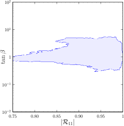
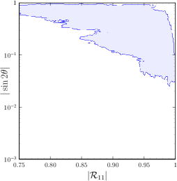
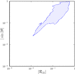
  • The analyses of Higgs signal strengths from the ATLAS and CMS collaborations, e.g. [24], put constraints on different couplings of hh{\rm h}. Overall, the resulting picture corresponds to an hh{\rm h} which is quite SM-like. For that reason, in order to discard from this simple analysis the regions of parameter space that these constraints will in any case eliminate in the complete analysis of section 6, we require here |11|0.9subscript110.9|\mathcal{R}_{11}|\geq 0.9.

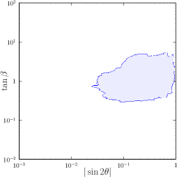
Although the analysis of section 3.4 already sets a lower bound |sin2θ|4×1032𝜃4superscript103|\sin 2\theta|\geq 4\times 10^{-3} in order to obtain the correct CKM matrix, we do not impose it here (it corresponds to the dashed vertical line in Figure 3(d)). A detailed discussion of one convenient parametrisation of all quantities related to the scalar sector is given in appendix B.1.
With these ingredients, the allowed regions in Figures 3 and 4 are obtained. We introduce

MMinmin(mH,mA,mH±),MMaxmax(mH,mA,mH±).formulae-sequencesubscript𝑀𝑀𝑖𝑛minsubscript𝑚Hsubscript𝑚Asubscript𝑚superscriptHplus-or-minussubscript𝑀𝑀𝑎𝑥maxsubscript𝑚Hsubscript𝑚Asubscript𝑚superscriptHplus-or-minusM_{Min}\equiv\text{min}(m_{{\rm H}},m_{{\rm A}},m_{{\rm H}^{\pm}}),\qquad M_{Max}\equiv\text{max}(m_{{\rm H}},m_{{\rm A}},m_{{\rm H}^{\pm}})\,. (72)

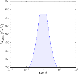
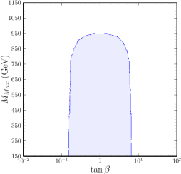
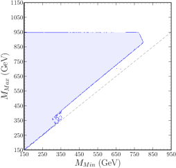
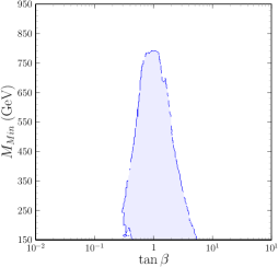
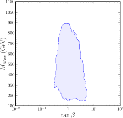
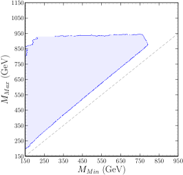
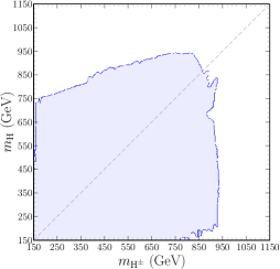
Figure 3(a) shows that, with the simple requirements enumerated above, all new scalars cannot have, simultaneously, masses above 750similar-toabsent750\sim 750 GeV. These values are in rough agreement with the previous naive estimates. Figure 3(b) shows in addition that no new scalar can be heavier than 950similar-toabsent950\sim 950 GeV. It is also clear that the largest values of the scalar masses correspond to tβ1similar-to-or-equalssubscript𝑡𝛽1t_{\beta}\simeq 1, while only a reduced range of values of tβsubscript𝑡𝛽t_{\beta} is allowed, 101<tβ<10superscript101subscript𝑡𝛽1010^{-1}<t_{\beta}<10.. Figure 3(c) shows that the limitations on allowed MMinsubscript𝑀𝑀𝑖𝑛M_{Min} and MMaxsubscript𝑀𝑀𝑎𝑥M_{Max} appear to be rather independent: for example, MMax850similar-tosubscript𝑀𝑀𝑎𝑥850M_{Max}\sim 850 GeV is compatible with any value of MMinsubscript𝑀𝑀𝑖𝑛M_{Min} below 750750750 GeV.
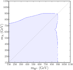
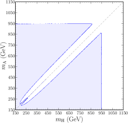
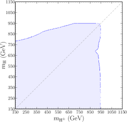
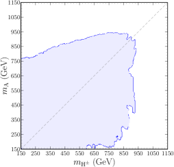
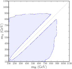
Figures 4(a)4(c) illustrate that any ordering of the masses mHsubscript𝑚Hm_{{\rm H}}, mAsubscript𝑚Am_{{\rm A}}, mH±subscript𝑚superscriptHplus-or-minusm_{{\rm H}^{\pm}} is allowed, and no particular restriction arises besides the impossibility of having mHmA>250similar-to-or-equalssubscript𝑚Hsubscript𝑚A250m_{{\rm H}}\simeq m_{{\rm A}}>250 GeV.

Refer to caption
(a) MMinsubscript𝑀𝑀𝑖𝑛M_{Min} vs. tanβ𝛽\tan\beta.
Refer to caption
(b) MMaxsubscript𝑀𝑀𝑎𝑥M_{Max} vs. tanβ𝛽\tan\beta.
Refer to caption
(c) MMaxsubscript𝑀𝑀𝑎𝑥M_{Max} vs. MMinsubscript𝑀𝑀𝑖𝑛M_{Min}.
Refer to caption
(d) tanβ𝛽\tan\beta vs. |sin2θ|2𝜃|\sin 2\theta|.
Figure 3: Regions allowed at 99% C.L. by the requirements on the scalar sector.
Refer to caption
(a) mAsubscript𝑚Am_{{\rm A}} vs. mH±subscript𝑚superscriptHplus-or-minusm_{{\rm H}^{\pm}}.
Refer to caption
(b) mAsubscript𝑚Am_{{\rm A}} vs. mHsubscript𝑚Hm_{{\rm H}}.
Refer to caption
(c) mHsubscript𝑚Hm_{{\rm H}} vs. mH±subscript𝑚superscriptHplus-or-minusm_{{\rm H}^{\pm}}.
Figure 4: Regions allowed at 99% C.L. by the requirements on the scalar sector.

Having introduced the physical scalars and analysed some relevant aspects of the scalar sector, we can now turn back to YsubscriptY\mathscr{L}_{\rm Y} in eq. (7) and discuss the Yukawa couplings of the physical quarks and scalars.

5 Physical Yukawa couplings

The Yukawa lagrangian in eq. (7)

Y=q¯q+Gq¯q+hq¯q+Hq¯q+Aq¯q+H±q¯q,subscriptYsubscript¯qqsubscript𝐺¯qqsubscripth¯qqsubscriptH¯qqsubscriptA¯qqsubscriptsuperscriptHplus-or-minus¯qq\mathscr{L}_{\rm Y}=\mathscr{L}_{{\rm\bar{q}q}}+\mathscr{L}_{G{\rm\bar{q}q}}+\mathscr{L}_{{\rm h}{\rm\bar{q}q}}+\mathscr{L}_{{\rm H}{\rm\bar{q}q}}+\mathscr{L}_{{\rm A}{\rm\bar{q}q}}+\mathscr{L}_{{\rm H}^{\pm}{\rm\bar{q}q}}, (73)

gives the mass terms for quarks q¯q=d¯LMddRu¯LMuuR+H.csubscript¯qqsubscript¯𝑑𝐿superscriptsubscript𝑀𝑑absentsubscript𝑑𝑅subscript¯𝑢𝐿superscriptsubscript𝑀𝑢absentsubscript𝑢𝑅H.c\mathscr{L}_{{\rm\bar{q}q}}=-\bar{d}_{L}M_{d}^{\phantom{\dagger}}d_{R}-\bar{u}_{L}M_{u}^{\phantom{\dagger}}u_{R}+\text{H.c}, the couplings to the would-be Goldstone bosons Gq¯qsubscript𝐺¯qq\mathscr{L}_{G{\rm\bar{q}q}},

Gq¯q=iG0v[d¯γ5du¯γ5u]2G+v[u¯LVMddRu¯RMuVdL]2Gv[d¯RMdVuLd¯LVMuuR],subscript𝐺¯qq𝑖superscript𝐺0𝑣delimited-[]¯𝑑subscript𝛾5𝑑¯𝑢subscript𝛾5𝑢2superscript𝐺𝑣delimited-[]subscript¯𝑢𝐿𝑉superscriptsubscript𝑀𝑑absentsubscript𝑑𝑅subscript¯𝑢𝑅superscriptsubscript𝑀𝑢absent𝑉subscript𝑑𝐿2superscript𝐺𝑣delimited-[]subscript¯𝑑𝑅superscriptsubscript𝑀𝑑absentsuperscript𝑉subscript𝑢𝐿subscript¯𝑑𝐿superscript𝑉superscriptsubscript𝑀𝑢absentsubscript𝑢𝑅\mathscr{L}_{G{\rm\bar{q}q}}=-i\frac{G^{0}}{v}\left[\bar{d}\gamma_{5}d-\bar{u}\gamma_{5}u\right]\\ -\frac{\sqrt{2}G^{+}}{v}\left[\bar{u}_{L}VM_{d}^{\phantom{\dagger}}d_{R}-\bar{u}_{R}M_{u}^{\phantom{\dagger}}Vd_{L}\right]-\frac{\sqrt{2}G^{-}}{v}\left[\bar{d}_{R}M_{d}^{\phantom{\dagger}}V^{\dagger}u_{L}-\bar{d}_{L}V^{\dagger}M_{u}^{\phantom{\dagger}}u_{R}\right], (74)

and the Yukawa couplings to the neutral and charged scalars Sq¯qsubscriptS¯qq\mathscr{L}_{{\rm S\bar{q}q}}, S=h𝑆hS={\rm h}, HH{\rm H}, AA{\rm A}, H±superscriptHplus-or-minus{\rm H}^{\pm}. Introducing the hermitian and antihermitian combinations

HqNq+Nq2,AqNqNq2,formulae-sequencesubscript𝐻𝑞superscriptsubscript𝑁𝑞absentsuperscriptsubscript𝑁𝑞2subscript𝐴𝑞superscriptsubscript𝑁𝑞absentsuperscriptsubscript𝑁𝑞2H_{q}\equiv\frac{N_{q}^{\phantom{\dagger}}+N_{q}^{\dagger}}{2},\quad A_{q}\equiv\frac{N_{q}^{\phantom{\dagger}}-N_{q}^{\dagger}}{2}, (75)

we have

Sq¯q=subscript𝑆¯qqabsent\displaystyle\mathscr{L}_{S{\rm\bar{q}q}}= Sv{d¯[1sMd+2sHd+i3sAd]d+d¯[2sAd+i3sHd]γ5d}𝑆𝑣¯𝑑delimited-[]subscript1𝑠superscriptsubscript𝑀𝑑absentsubscript2𝑠subscript𝐻𝑑𝑖subscript3𝑠subscript𝐴𝑑𝑑¯𝑑delimited-[]subscript2𝑠subscript𝐴𝑑𝑖subscript3𝑠subscript𝐻𝑑subscript𝛾5𝑑\displaystyle-\frac{S}{v}\left\{\bar{d}\left[\mathcal{R}_{1s}M_{d}^{\phantom{\dagger}}+\mathcal{R}_{2s}H_{d}+i\mathcal{R}_{3s}A_{d}\right]d+\bar{d}\left[\mathcal{R}_{2s}A_{d}+i\mathcal{R}_{3s}H_{d}\right]\gamma_{5}d\right\}
Sv{u¯[1sMu+2sHui3sAu]u+u¯[2sAui3sHu]γ5u},𝑆𝑣¯𝑢delimited-[]subscript1𝑠superscriptsubscript𝑀𝑢absentsubscript2𝑠subscript𝐻𝑢𝑖subscript3𝑠subscript𝐴𝑢𝑢¯𝑢delimited-[]subscript2𝑠subscript𝐴𝑢𝑖subscript3𝑠subscript𝐻𝑢subscript𝛾5𝑢\displaystyle-\frac{S}{v}\left\{\bar{u}\left[\mathcal{R}_{1s}M_{u}^{\phantom{\dagger}}+\mathcal{R}_{2s}H_{u}-i\mathcal{R}_{3s}A_{u}\right]u+\bar{u}\left[\mathcal{R}_{2s}A_{u}-i\mathcal{R}_{3s}H_{u}\right]\gamma_{5}u\right\}, (76)

with s=1,2,3𝑠123s=1,2,3 for S=h,H,A𝑆hHAS={\rm h},{\rm H},{\rm A}, respectively, and

H±q¯q=2H+v[u¯LVNddRu¯RNuVdL]2Hv[d¯RNdVuLd¯LVNuuR].subscriptsuperscriptHplus-or-minus¯qq2superscriptH𝑣delimited-[]subscript¯𝑢𝐿𝑉superscriptsubscript𝑁𝑑absentsubscript𝑑𝑅subscript¯𝑢𝑅superscriptsubscript𝑁𝑢𝑉subscript𝑑𝐿2superscriptH𝑣delimited-[]subscript¯𝑑𝑅superscriptsubscript𝑁𝑑superscript𝑉subscript𝑢𝐿subscript¯𝑑𝐿superscript𝑉superscriptsubscript𝑁𝑢absentsubscript𝑢𝑅\mathscr{L}_{{\rm H}^{\pm}{\rm\bar{q}q}}=-\frac{\sqrt{2}{\rm H}^{+}}{v}\left[\bar{u}_{L}VN_{d}^{\phantom{\dagger}}d_{R}-\bar{u}_{R}N_{u}^{\dagger}Vd_{L}\right]-\frac{\sqrt{2}{\rm H}^{-}}{v}\left[\bar{d}_{R}N_{d}^{\dagger}V^{\dagger}u_{L}-\bar{d}_{L}V^{\dagger}N_{u}^{\phantom{\dagger}}u_{R}\right]. (77)

With eqs. (29)–(30), [Hq]ijsubscriptdelimited-[]subscript𝐻𝑞𝑖𝑗[H_{q}]_{ij} and [Aq]ijsubscriptdelimited-[]subscript𝐴𝑞𝑖𝑗[A_{q}]_{ij} in eq. (75) read

[Hq]ijsubscriptdelimited-[]subscript𝐻𝑞𝑖𝑗\displaystyle[H_{q}]_{ij} =tβδijmqi(tβ+tβ1)n^[q]in^[q]jmdi+mdj2,absentsubscript𝑡𝛽subscript𝛿𝑖𝑗subscript𝑚subscript𝑞𝑖subscript𝑡𝛽superscriptsubscript𝑡𝛽1superscriptsubscript^𝑛delimited-[]q𝑖superscriptsubscript^𝑛delimited-[]q𝑗absentsubscript𝑚subscript𝑑𝑖subscript𝑚subscript𝑑𝑗2\displaystyle=t_{\beta}\delta_{ij}m_{q_{i}}-(t_{\beta}+t_{\beta}^{-1})\hat{n}_{{\rm[q]}i}^{\ast}\hat{n}_{{\rm[q]}j}^{\phantom{\ast}}\frac{m_{d_{i}}+m_{d_{j}}}{2}, (78)
[Aq]ijsubscriptdelimited-[]subscript𝐴𝑞𝑖𝑗\displaystyle[A_{q}]_{ij} =(tβ+tβ1)n^[q]in^[q]jmdimdj2.absentsubscript𝑡𝛽superscriptsubscript𝑡𝛽1superscriptsubscript^𝑛delimited-[]q𝑖superscriptsubscript^𝑛delimited-[]q𝑗absentsubscript𝑚subscript𝑑𝑖subscript𝑚subscript𝑑𝑗2\displaystyle=(t_{\beta}+t_{\beta}^{-1})\hat{n}_{{\rm[q]}i}^{\ast}\hat{n}_{{\rm[q]}j}^{\phantom{\ast}}\frac{m_{d_{i}}-m_{d_{j}}}{2}. (79)

We recall – see for example [25] – that, for flavour changing Yukawa couplings of quarks qjsubscript𝑞𝑗q_{j}, qksubscript𝑞𝑘q_{k} and a scalar S𝑆S, of the form

Sqjqk=Sq¯j(ajk+ibjkγ5)qk+H.c,ajk,bjk,formulae-sequencesubscriptsubscriptSqjsubscriptqk𝑆subscript¯𝑞𝑗subscript𝑎𝑗𝑘𝑖subscript𝑏𝑗𝑘subscript𝛾5subscript𝑞𝑘H.csubscript𝑎𝑗𝑘subscript𝑏𝑗𝑘\mathscr{L}_{{\rm Sq_{j}q_{k}}}=-S\bar{q}_{j}(a_{jk}+ib_{jk}\gamma_{5})q_{k}+\text{H.c},\quad a_{jk},b_{jk}\in\mathbb{C}, (80)

CP conservation requires Re(ajkbjk)=0Resuperscriptsubscript𝑎𝑗𝑘subscript𝑏𝑗𝑘0\text{Re}\left(a_{jk}^{\ast}b_{jk}\right)=0. In this model

Re(ajkbjk)2s3s(tβ+tβ1)2mqjmqk|n^[q]jn^[q]k|2,proportional-toResuperscriptsubscript𝑎𝑗𝑘subscript𝑏𝑗𝑘subscript2𝑠subscript3𝑠superscriptsubscript𝑡𝛽superscriptsubscript𝑡𝛽12subscript𝑚subscript𝑞𝑗subscript𝑚subscript𝑞𝑘superscriptsuperscriptsubscript^𝑛delimited-[]q𝑗superscriptsubscript^𝑛delimited-[]q𝑘absent2\text{Re}\left(a_{jk}^{\ast}b_{jk}\right)\propto\mathcal{R}_{2s}\mathcal{R}_{3s}(t_{\beta}+t_{\beta}^{-1})^{2}m_{q_{j}}m_{q_{k}}|\hat{n}_{{\rm[q]}j}^{\ast}\hat{n}_{{\rm[q]}k}^{\phantom{\ast}}|^{2}\,, (81)

and thus, with \mathcal{R} mixing all three neutral scalars, the flavour changing Yukawa couplings are CP violating. For the charged scalar, we have

Re(ajkbjk)Im((VNd)jk(NuV)jk),proportional-toResuperscriptsubscript𝑎𝑗𝑘subscript𝑏𝑗𝑘Imsuperscriptsubscript𝑉superscriptsubscript𝑁𝑑absent𝑗𝑘subscriptsuperscriptsubscript𝑁𝑢𝑉𝑗𝑘\text{Re}\left(a_{jk}^{\ast}b_{jk}\right)\propto\text{Im}\left((VN_{d}^{\phantom{\dagger}})_{jk}^{\ast}(N_{u}^{\dagger}V)_{jk}\right)\,, (82)

and thus in general, even for real Nqsuperscriptsubscript𝑁𝑞absentN_{q}^{\phantom{\dagger}}, the Yukawa couplings of H±superscriptHplus-or-minus{\rm H}^{\pm} are also CP violating.
For flavour conserving Yukawa couplings

Sqq=Sq¯(a+ibγ5)q,a,b,formulae-sequencesubscriptSqq𝑆¯𝑞𝑎𝑖𝑏subscript𝛾5𝑞𝑎𝑏\mathscr{L}_{{\rm Sqq}}=-S\bar{q}(a+ib\gamma_{5})q,\quad a,b\in\mathbb{R}, (83)

CP conservation requires ab=0𝑎𝑏0ab=0. Then, for the coupling of the neutral scalar S𝑆S, with eqs. (78)–(79), we have

ab3smqj2(1s+2s[tβ(tβ+tβ1)|n^[q]j|2])(tβ(tβ+tβ1)|n^[q]j|2),proportional-to𝑎𝑏subscript3𝑠superscriptsubscript𝑚subscript𝑞𝑗2subscript1𝑠subscript2𝑠delimited-[]subscript𝑡𝛽subscript𝑡𝛽superscriptsubscript𝑡𝛽1superscriptsuperscriptsubscript^𝑛delimited-[]q𝑗absent2subscript𝑡𝛽subscript𝑡𝛽superscriptsubscript𝑡𝛽1superscriptsuperscriptsubscript^𝑛delimited-[]q𝑗absent2ab\propto\mathcal{R}_{3s}m_{q_{j}}^{2}\left(\mathcal{R}_{1s}+\mathcal{R}_{2s}[t_{\beta}-(t_{\beta}+t_{\beta}^{-1})|\hat{n}_{{\rm[q]}j}^{\phantom{\ast}}|^{2}]\right)\left(t_{\beta}-(t_{\beta}+t_{\beta}^{-1})|\hat{n}_{{\rm[q]}j}^{\phantom{\ast}}|^{2}\right)\,, (84)

and thus the flavour conserving Yukawa couplings violate CP as long as the mixing in the scalar sector connects AA{\rm A} with hh{\rm h}, HH{\rm H}. Contributions to the electric dipole moment of the neutron arise from eq. (84), but the suppression due to the mqj2superscriptsubscript𝑚subscript𝑞𝑗2m_{q_{j}}^{2} factor for qj=u,dsubscript𝑞𝑗𝑢𝑑q_{j}=u,d, together with the need of different non-zero mixings in the scalar sector, keep them within experimental bounds [26].

6 Phenomenology

6.1 Analysis and constraints

In section 3 we have shown that the model can give a CKM mixing matrix in agreement with data. We have also explored some aspects of the scalar sector in section 4. In this section we analyse the model considering simultaneously (i) obtention of an adequate CKM matrix (moduli |Vij|superscriptsubscript𝑉𝑖𝑗absent|{V_{ij}^{\phantom{\ast}}}| in the first and second rows and phase γ𝛾\gamma in agreement with data), (ii) a scalar sector verifying boundedness, perturbative unitarity, oblique parameter constraints and mHsubscript𝑚Hm_{{\rm H}}, mAsubscript𝑚Am_{{\rm A}}, mH±>150subscript𝑚superscriptHplus-or-minus150m_{{\rm H}^{\pm}}>150 GeV, and (iii) a number of constraints, to be discussed in the following, which involve both the quark Yukawa couplings and the scalar sector.

  • Production ×\times decay signal strengths of the 125 GeV Higgs-like scalar hh{\rm h}.
    Agreement with the combined results of ATLAS and CMS from the LHC-Run I [24], together with additional data, involving in particular hbb¯h𝑏¯𝑏{\rm h}\to b\bar{b} [27, 28] from LHC-Run II, constrains the scalar mixings j1subscript𝑗1\mathcal{R}_{j1} and the diagonal entries of the Ndsuperscriptsubscript𝑁𝑑absentN_{d}^{\phantom{\dagger}} and Nusuperscriptsubscript𝑁𝑢absentN_{u}^{\phantom{\dagger}} matrices (see, for example, [29]). Notice that the requirement |11|0.9subscript110.9|\mathcal{R}_{11}|\geq 0.9 used in section 4 to mimic coarsely the effect of these results is, of course, not imposed here.

  • Neutral meson mixings.
    One of the most relevant characteristics of the model is the presence of tree level flavour changing couplings of the neutral scalars: they produce the contributions to neutral meson mixing represented in Figure 5(a). They affect mass differences and CP violating observables [22, 30]. For Bd0superscriptsubscript𝐵𝑑0B_{d}^{0}B¯d0superscriptsubscript¯𝐵𝑑0\bar{B}_{d}^{0} and Bs0superscriptsubscript𝐵𝑠0B_{s}^{0}B¯s0superscriptsubscript¯𝐵𝑠0\bar{B}_{s}^{0} we impose agreement with the mass differences ΔMBdΔsubscript𝑀subscript𝐵𝑑\Delta M_{B_{d}}, ΔMBsΔsubscript𝑀subscript𝐵𝑠\Delta M_{B_{s}} and the mixing ×\times decay CP asymmetries in BdJ/ΨKSsubscript𝐵𝑑𝐽Ψsubscript𝐾𝑆B_{d}\to J/\Psi K_{S} and BsJ/ΨΦsubscript𝐵𝑠𝐽ΨΦB_{s}\to J/\Psi\Phi, respectively. For K0superscript𝐾0K^{0}K¯0superscript¯𝐾0\bar{K}^{0}, we impose that the scalar mediated short distance contribution to M12Ksuperscriptsubscript𝑀12𝐾M_{12}^{K} does not yield sizable contributions to ϵKsubscriptitalic-ϵ𝐾\epsilon_{K} and ΔMKΔsubscript𝑀𝐾\Delta M_{K}; in particular, for ΔMKΔsubscript𝑀𝐾\Delta M_{K}, we require 2|M12K|SFCNC<ΔMK2subscriptsuperscriptsubscript𝑀12𝐾𝑆𝐹𝐶𝑁𝐶Δsubscript𝑀𝐾2|M_{12}^{K}|_{SFCNC}<\Delta M_{K}. For D0superscript𝐷0D^{0}D¯0superscript¯𝐷0\bar{D}^{0}, we impose, similarly, that the short distance contribution to M12Dsuperscriptsubscript𝑀12𝐷M_{12}^{D} verifies |M12D|<3×10²ps1superscriptsubscript𝑀12𝐷3superscript102superscriptps1|M_{12}^{D}|<3\times 10^{-2}\,\text{ps}^{-1}. In summary, neutral meson mixings constrain scalar mixings ijsubscript𝑖𝑗\mathcal{R}_{ij} and masses, together with off-diagonal entries of Ndsuperscriptsubscript𝑁𝑑absentN_{d}^{\phantom{\dagger}} and the 121212, 212121, elements of Nusuperscriptsubscript𝑁𝑢absentN_{u}^{\phantom{\dagger}}.
    Besides the SM one loop contribution, we only consider the scalar mediated tree level contributions to the Wilson coefficients of the different operators of interest; their QCD evolution from the electroweak scale to low energies follows [31, 32, 33]. For the operator matrix elements and bag factors, we use [34] and [35] (see also [36]).

  • bsγ𝑏𝑠𝛾b\to s\gamma.
    One loop diagrams like, for example, the ones in Figure 5(b), contribute to Br(BXsγ)Br𝐵subscript𝑋𝑠𝛾\text{Br}(B\to X_{s}\gamma), and further constrain Nusuperscriptsubscript𝑁𝑢absentN_{u}^{\phantom{\dagger}} and Ndsuperscriptsubscript𝑁𝑑absentN_{d}^{\phantom{\dagger}}, the neutral scalar mixings and masses, and mH±subscript𝑚superscriptHplus-or-minusm_{{\rm H}^{\pm}} (in the previous constraints mH±subscript𝑚superscriptHplus-or-minusm_{{\rm H}^{\pm}} does only appear in the one loop hγγh𝛾𝛾{\rm h}\to\gamma\gamma amplitude). Details of the calculation follow [37, 38].

  • Rare top decays thq𝑡h𝑞t\to{\rm h}q.
    Current bounds [39, 40, 41] on thc,hu𝑡h𝑐h𝑢t\to{\rm h}c,{\rm h}u are at the 103superscript10310^{-3} level, and have to be included in the analysis.

Refer to caption

(a)
Refer to caption
(b)
Figure 5: Diagrams contributing to: (a) meson mixing, (b) bsγ𝑏𝑠𝛾b\to s\gamma.

The analysis has two main goals:

  1. 1.

    to establish that the model is viable after a reasonable set of constraints is imposed;

  2. 2.

    to explore the prospects for the observation of some definite non-SM signal. We concentrate in particular on flavour changing decays thc,hu𝑡h𝑐h𝑢t\to{\rm h}c,{\rm h}u and hbs,bdh𝑏𝑠𝑏𝑑{\rm h}\to bs,bd, of interest, respectively, for the LHC and the ILC [42]. These are the most interesting tree level induced neutral flavour changing decays, since huc,dsh𝑢𝑐𝑑𝑠{\rm h}\to uc,ds are more suppressed by the light fermion mass factors in Nusuperscriptsubscript𝑁𝑢absentN_{u}^{\phantom{\dagger}} and Ndsuperscriptsubscript𝑁𝑑absentN_{d}^{\phantom{\dagger}} (in addition, the experimental analysis is also more difficult having only light quarks in the final state).
    We also consider a representative low energy observable, the time dependent CP violating asymmetry in BsJ/ΨΦsubscript𝐵𝑠𝐽ΨΦB_{s}\to J/\Psi\Phi, AJ/ΨΦCPsubscriptsuperscript𝐴𝐶𝑃𝐽ΨΦA^{CP}_{J/\Psi\Phi}, for which the SM prediction is AJ/ΨΦCP0.04similar-to-or-equalssubscriptsuperscript𝐴𝐶𝑃𝐽ΨΦ0.04A^{CP}_{J/\Psi\Phi}\simeq-0.04, while current results [43] give 0.030±0.033plus-or-minus0.0300.033-0.030\pm 0.033, leaving significant room for New Physics contributions.

Further implications for the phenomenology of HH{\rm H}, AA{\rm A} and H±superscriptHplus-or-minus{\rm H}^{\pm}, vary significantly between allowed regions in the parameter space of the model (for example, the relevant decay modes change depending on which scalar is heavier and on the values of the Nqsuperscriptsubscript𝑁𝑞absentN_{q}^{\phantom{\dagger}} matrices), and would also involve, and be sensitive to, the couplings of the scalars with leptons, which we have not discussed in this work. As commented in precedence, we do not address such implications here. The fact that we have not included a description of the leptonic sector prevents (i) the use of constraints such as, for example, Br(Bsμ+μ)Brsubscript𝐵𝑠superscript𝜇superscript𝜇\text{Br}(B_{s}\to\mu^{+}\mu^{-}) or Br(KLμ+μ)Brsubscript𝐾𝐿superscript𝜇superscript𝜇\text{Br}(K_{L}\to\mu^{+}\mu^{-}), and (ii) considerations on potential New Physics signals which involve leptons, as the so-called “B anomalies” [44].

6.2 Results

The main results of the full analysis are presented in Figures 6 to 11.
Figure 6(a) corresponds to Figures 2(d)2(f) of the analysis in section 3: as one could anticipate, it is to be noticed that the allowed regions, where the model satisfies all the constraints, are much reduced with respect to the simple requirement of section 3, i.e. just reproducing a realistic CKM matrix. In particular, the only allowed regions for θdsubscript𝜃𝑑\theta_{d} and φdsubscript𝜑𝑑\varphi_{d} correspond to having one component of r^[d]subscript^𝑟delimited-[]d\hat{r}_{{\rm[d]}} close to ±1plus-or-minus1\pm 1 (that is close to the points (0,±1)0plus-or-minus1(0,\pm 1), (±1,0)plus-or-minus10(\pm 1,0), (0,0)00(0,0) in Figure 6(a)), and the remaining two components much smaller: this naturally suppresses neutral flavour changing couplings, since they depend on the products of different components. As discussed in subsection 3.2 and in appendix A, without actually reaching that exact point, at which the CKM matrix becomes CP conserving. From this point of vue, those regions are “close to” (but not exactly) the different types of BGL models (as discussed in [12]), in which (i) tree SFCNC are absent in one of the quark sectors and (ii) the scalar potential does not permit spontaneous CP violation. This is clearly illustrated by Figures 6(d), 6(e) and 6(f), that are enlargements of Figure 6(a) with peculiar logarithmic scales where values below 103superscript10310^{-3} have been collapsed to the central point. These central points correspond, respectively, to the flavour structures of the BGL models of types d𝑑d, s𝑠s and b𝑏b. For example, the b𝑏b BGL model corresponds to r^[d]=(0,0,±1)subscript^𝑟delimited-[]d00plus-or-minus1\hat{r}_{{\rm[d]}}=(0,0,\pm 1). The figures show that the allowed regions exclude the BGL models, but remain close. Correspondingly, the regions close to the flavour structures of up type BGL models (which are also indicated in the Figures), remain empty, i.e. they are not allowed. For example, the t𝑡t BGL model corresponds to the small holes in the allowed region in Figure 6(f).
Figures 6(b) and 6(c) correspond to Figures 2(b) and 2(c) in subsection 3.4: the range of allowed values for |r^[d]Mid|subscript^𝑟delimited-[]d𝑀𝑖𝑑|\hat{r}_{{\rm[d]}Mid}|, |r^[u]Mid|subscript^𝑟delimited-[]u𝑀𝑖𝑑|\hat{r}_{{\rm[u]}Mid}| is reduced in the full analysis, in particular the largest allowed values are now smaller than 0.30.30.3.
Figure 7 corresponds to Figure 3 of the analysis of the scalar sector in section 4. It is clear that the constraints of the full analysis reduce the available room for tβsubscript𝑡𝛽t_{\beta}, leaving only 1/4<tβ<414subscript𝑡𝛽41/4<t_{\beta}<4. Furthermore, the allowed region in MMaxsubscript𝑀𝑀𝑎𝑥M_{Max} vs. MMinsubscript𝑀𝑀𝑖𝑛M_{Min} in Fig. 7(c) is slightly reduced with respect to Fig. 3(c). Notice in particular that the region with all new scalars light, i.e. MMax<250subscript𝑀𝑀𝑎𝑥250M_{Max}<250 GeV, is now almost excluded. On the contrary, the largest values of MMaxsubscript𝑀𝑀𝑎𝑥M_{Max} and MMinsubscript𝑀𝑀𝑖𝑛M_{Min} coincide with those in section 4, that is, they are still limited by the requirements on the scalar sector itself. The same comments apply to Figure 8, which corresponds to Figure 4 of the analysis of section 4. Notice that |sin2θ|2𝜃|\sin 2\theta| is now required to be in the range [0.03;1.0]0.031.0[0.03;1.0].
Figure 9(a) shows that deviations from |11|=1subscript111|\mathcal{R}_{11}|=1 can be achieved for almost all values of tβsubscript𝑡𝛽t_{\beta} within the allowed range, while Figures 9(b) and 9(c) illustrate, as expected, that for large values of |sin2θ|2𝜃|\sin 2\theta|, 31subscript31\mathcal{R}_{31} (which controls the amount of pseudoscalar I0superscript𝐼0{I}^{0} entering hh{\rm h}), reaches the larger allowed values, while |11|subscript11|\mathcal{R}_{11}| is reduced. Notice in particular that, overall, |31|102subscript31superscript102|\mathcal{R}_{31}|\geq 10^{-2} and that values as large as |31|0.4similar-tosubscript310.4|\mathcal{R}_{31}|\sim 0.4 are allowed. In any case, even if |11|subscript11|\mathcal{R}_{11}| can reach values very close to 111, |11|<1subscript111|\mathcal{R}_{11}|<1.

Refer to caption
(a) sθdsφdsubscript𝑠subscript𝜃𝑑subscript𝑠subscript𝜑𝑑s_{\theta_{d}}s_{\varphi_{d}} vs. sθdcφdsubscript𝑠subscript𝜃𝑑subscript𝑐subscript𝜑𝑑s_{\theta_{d}}c_{\varphi_{d}}
Refer to caption
(b) |r^[d]Min|subscript^𝑟delimited-[]d𝑀𝑖𝑛|\hat{r}_{{\rm[d]}Min}| vs. |r^[d]Mid|subscript^𝑟delimited-[]d𝑀𝑖𝑑|\hat{r}_{{\rm[d]}Mid}|.
Refer to caption
(c) |r^[u]Min|subscript^𝑟delimited-[]u𝑀𝑖𝑛|\hat{r}_{{\rm[u]}Min}| vs. |r^[u]Mid|subscript^𝑟delimited-[]u𝑀𝑖𝑑|\hat{r}_{{\rm[u]}Mid}|.
Refer to caption
(d) r^[d]3subscript^𝑟delimited-[]d3\hat{r}_{{\rm[d]}3} vs. r^[d]2subscript^𝑟delimited-[]d2\hat{r}_{{\rm[d]}2}
Refer to caption
(e) r^[d]3subscript^𝑟delimited-[]d3\hat{r}_{{\rm[d]}3} vs. r^[d]1subscript^𝑟delimited-[]d1\hat{r}_{{\rm[d]}1}
Refer to caption
(f) r^[d]2subscript^𝑟delimited-[]d2\hat{r}_{{\rm[d]}2} vs. r^[d]1subscript^𝑟delimited-[]d1\hat{r}_{{\rm[d]}1}
Figure 6: Regions allowed at 99% C.L. by the requirements of the full analysis.
Refer to caption
(a) MMinsubscript𝑀𝑀𝑖𝑛M_{Min} vs. tanβ𝛽\tan\beta.
Refer to caption
(b) MMaxsubscript𝑀𝑀𝑎𝑥M_{Max} vs. tanβ𝛽\tan\beta.
Refer to caption
(c) MMaxsubscript𝑀𝑀𝑎𝑥M_{Max} vs. MMinsubscript𝑀𝑀𝑖𝑛M_{Min}.
Refer to caption
(d) tanβ𝛽\tan\beta vs. |sin2θ|2𝜃|\sin 2\theta|.
Figure 7: Regions allowed at 99% C.L. by the requirements of the full analysis.
Refer to caption
(a) mAsubscript𝑚Am_{{\rm A}} vs. mH±subscript𝑚superscriptHplus-or-minusm_{{\rm H}^{\pm}}.
Refer to caption
(b) mAsubscript𝑚Am_{{\rm A}} vs. mHsubscript𝑚Hm_{{\rm H}}.
Refer to caption
(c) mHsubscript𝑚Hm_{{\rm H}} vs. mH±subscript𝑚superscriptHplus-or-minusm_{{\rm H}^{\pm}}.
Figure 8: Regions allowed at 99% C.L. by the requirements of the full analysis.
Refer to caption
(a) tβsubscript𝑡𝛽t_{\beta} vs. |11|subscript11|\mathcal{R}_{11}|.
Refer to caption
(b) |sin2θ|2𝜃|\sin 2\theta| vs. |11|subscript11|\mathcal{R}_{11}|.
Refer to caption
(c) |sin2θ|2𝜃|\sin 2\theta| vs. 31subscript31\mathcal{R}_{31}.
Figure 9: Regions allowed at 99% C.L. by the requirements of the full analysis.

Finally, Figures 10 and 11 illustrate some New Physics prospects in different flavour changing neutral transitions.
Figure 10(a) shows999The notation is Br(hbs)Br(hb¯s+bs¯)Brh𝑏𝑠Brh¯𝑏𝑠𝑏¯𝑠\text{Br}({\rm h}\to bs)\equiv\text{Br}({\rm h}\to\bar{b}s+b\bar{s}), Br(hbd)Br(hb¯d+bd¯)Brh𝑏𝑑Brh¯𝑏𝑑𝑏¯𝑑\text{Br}({\rm h}\to bd)\equiv\text{Br}({\rm h}\to\bar{b}d+b\bar{d}), etc. Br(hbs)Brh𝑏𝑠\text{Br}({\rm h}\to bs) vs. AJ/ΨΦCPsubscriptsuperscript𝐴𝐶𝑃𝐽ΨΦA^{CP}_{J/\Psi\Phi}; it is interesting to notice that: (i) Br(hbs)Brh𝑏𝑠\text{Br}({\rm h}\to bs) can reach values as large as 102superscript10210^{-2}, relevant for searches at the ILC, and (ii) significant deviations of the SM expectation AJ/ΨΦCP0.036similar-to-or-equalssubscriptsuperscript𝐴𝐶𝑃𝐽ΨΦ0.036A^{CP}_{J/\Psi\Phi}\simeq-0.036 can arise. An interesting correlation among New Physics effects follows: AJ/ΨΦCPsubscriptsuperscript𝐴𝐶𝑃𝐽ΨΦA^{CP}_{J/\Psi\Phi} values neatly different from SM expectations (the dashed vertical line in Figure 10(a)) would necessarily require values of Br(hbs)Brh𝑏𝑠\text{Br}({\rm h}\to bs) in the range 104superscript10410^{-4}-102superscript10210^{-2}. The origin of such a correlation is clear: the tree level couplings that induce hbsh𝑏𝑠{\rm h}\to bs at that level also contribute significantly to the dispersive amplitude M12Bssuperscriptsubscript𝑀12subscript𝐵𝑠M_{12}^{B_{s}} in Bs0subscriptsuperscript𝐵0𝑠B^{0}_{s}B¯s0subscriptsuperscript¯𝐵0𝑠\bar{B}^{0}_{s} mixing, changing its phase while maintaining |M12Bs|superscriptsubscript𝑀12subscript𝐵𝑠|M_{12}^{B_{s}}| (i.e. ΔMBsΔsubscript𝑀subscript𝐵𝑠\Delta M_{B_{s}}). According to the discussion on the connection of SFCNC and CP violation in subsection 3.2, tree level SFCNC should give

Br(thc)+Br(thu)+Br(hcu)0andBr𝑡h𝑐Br𝑡h𝑢Brh𝑐𝑢0and\displaystyle\text{Br}(t\to{\rm h}c)+\text{Br}(t\to{\rm h}u)+\text{Br}({\rm h}\to cu)\neq 0\qquad\text{and}
Br(hbs)+Br(hbd)+Br(hsd)0.Brh𝑏𝑠Brh𝑏𝑑Brh𝑠𝑑0\displaystyle\text{Br}({\rm h}\to bs)+\text{Br}({\rm h}\to bd)+\text{Br}({\rm h}\to sd)\neq 0\,. (85)

We introduce

Br(thq)Br(thc)+Br(thu),Br𝑡h𝑞Br𝑡h𝑐Br𝑡h𝑢\displaystyle\text{Br}(t\to{\rm h}q)\equiv\text{Br}(t\to{\rm h}c)+\text{Br}(t\to{\rm h}u),
Br(hbq)Br(hbs)+Br(hbd),Brh𝑏𝑞Brh𝑏𝑠Brh𝑏𝑑\displaystyle\text{Br}({\rm h}\to bq)\equiv\text{Br}({\rm h}\to bs)+\text{Br}({\rm h}\to bd),
Br(hq1q2)Br(hbq)+Br(hsd)+Br(hcu).Brhsubscript𝑞1subscript𝑞2Brh𝑏𝑞Brh𝑠𝑑Brh𝑐𝑢\displaystyle\text{Br}({\rm h}\to q_{1}q_{2})\equiv\text{Br}({\rm h}\to bq)+\text{Br}({\rm h}\to sd)+\text{Br}({\rm h}\to cu). (86)

Concentrating on the decays of hh{\rm h}, eq. (85) implies, for the total rate of flavour changing decays of hh{\rm h} Br(hq1q2)Brhsubscript𝑞1subscript𝑞2\text{Br}({\rm h}\to q_{1}q_{2}), Br(hq1q2)0Brhsubscript𝑞1subscript𝑞20\text{Br}({\rm h}\to q_{1}q_{2})\neq 0. Figure 10(b) clearly shows that in any case 5×10⁶Br(hq1q2)2×1025superscript106Brhsubscript𝑞1subscript𝑞22superscript1025\times 10^{-6}\leq\text{Br}({\rm h}\to q_{1}q_{2})\leq 2\times 10^{-2}.
Figure 11 shows different correlations among the branching ratios of flavour changing transitions involving hh{\rm h}. It is important to notice that these New Physics signals are not confined to one particular sector (up or down type quarks) and that the largest allowed rates can be achieved for the transitions with second and third generation quarks, thc𝑡h𝑐t\to{\rm h}c and hbsh𝑏𝑠{\rm h}\to bs. Notice in particular that for thc𝑡h𝑐t\to{\rm h}c, the LHC bounds at the level of 103superscript10310^{-3} do play a role in limiting the allowed regions. Of course, the remaining transitions, thu𝑡h𝑢t\to{\rm h}u and hbd,sd,cuh𝑏𝑑𝑠𝑑𝑐𝑢{\rm h}\to bd,sd,cu are also interesting: even if the largest values of their rates are smaller than the largest values allowed for thc𝑡h𝑐t\to{\rm h}c and hbsh𝑏𝑠{\rm h}\to bs, in some regions of the parameter space they have larger rates than thc𝑡h𝑐t\to{\rm h}c and hbsh𝑏𝑠{\rm h}\to bs, and they can also be within experimental reach.
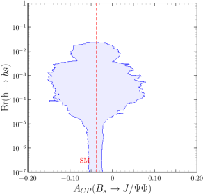
Refer to caption
(a) Br(hbs)Brh𝑏𝑠\text{Br}({\rm h}\to bs) vs. AJ/ΨΦCPsubscriptsuperscript𝐴𝐶𝑃𝐽ΨΦA^{CP}_{J/\Psi\Phi}.
Refer to caption
(b) Br(hq1q2)Brhsubscript𝑞1subscript𝑞2\text{Br}({\rm h}\to q_{1}q_{2}) vs. tβsubscript𝑡𝛽t_{\beta}.
Figure 10: Region allowed at 99% C.L. by the requirements of the full analysis.
Refer to caption
(a) thq𝑡h𝑞t\to{\rm h}q vs. hq1q2hsubscript𝑞1subscript𝑞2{\rm h}\to q_{1}q_{2}.
Refer to caption
(b) thq𝑡h𝑞t\to{\rm h}q vs. hbqh𝑏𝑞{\rm h}\to bq.
Refer to caption
(c) hq1q2hsubscript𝑞1subscript𝑞2{\rm h}\to q_{1}q_{2} vs. hbqh𝑏𝑞{\rm h}\to bq.
Refer to caption
(d) thu𝑡h𝑢t\to{\rm h}u vs. thc𝑡h𝑐t\to{\rm h}c.
Refer to caption
(e) hbdh𝑏𝑑{\rm h}\to bd vs. hbsh𝑏𝑠{\rm h}\to bs.
Refer to caption
(f) thc𝑡h𝑐t\to{\rm h}c vs. hbsh𝑏𝑠{\rm h}\to bs.
Figure 11: Regions allowed at 99% C.L. by the requirements of the full analysis.

Conclusions

In this paper we have addressed the question: is it possible to construct a realistic model with spontaneous CP violation, in the framework of a minimal two Higgs doublet extension of the Standard Model? We show that this is indeed possible. In order to accomplish this task, one has to surmount enormous obstacles, like having a natural suppression of SFCNC and generating a complex CKM matrix from the vacuum phase, with the correct strength of the invariant measure of the amount of CP violation in the quark mixing matrix.

We have shown that a minimal scenario is phenomenological viable, through the introduction of a flavoured 2subscript2\mathbb{Z}_{2} symmetry, where one of the three quark families is odd under 2subscript2\mathbb{Z}_{2} while the other two are even. A remarkable feature of the model is its prediction of New Physics which can be discovered at the LHC. More precisely, the model predicts that all the new scalars have a mass below 950 GeV with at least one of the masses below 750 GeV. This prediction is obtained through a thorough study of the constraints arising from the 125 GeV Higgs signals, the size of neutral meson mixings, the size of bsγ𝑏𝑠𝛾b\to s\gamma, and reproducing a correct CKM matrix, including the size of CP violation. Constraints from the electroweak oblique parameters, and perturbative unitarity and boundedness of the scalar potential are also included.
We encounter a deep connection between the generation of a complex CKM matrix from a vacuum phase and the necessary appearance of SFCNC. In the New Physics predictions, we give special emphasis to processes like thc,hu𝑡h𝑐h𝑢t\to{\rm h}c,{\rm h}u, hbs,bd𝑏𝑠𝑏𝑑h\to bs,bd, which are relevant for the LHC and the ILC. Interestingly, there is still room for important New Physics contributions to the phase of Bs0superscriptsubscript𝐵𝑠0B_{s}^{0}B¯s0superscriptsubscript¯𝐵𝑠0\bar{B}_{s}^{0} mixing.

In the present model of SCPV, none of the new scalars can be heavier than 1 TeV, and the presence of SFCNC cannot be avoided. The experimental constraints select regions in parameter space where the SFCNC are kept under control, as happens in BGL models. It is indeed remarkable that these allowed regions are located close to BGL models: for example, in the neighbourhood of a down-type BGL flavour structure, we almost do not have SFCNC in the down sector while the SFCNC in the up sector are of the Minimal Flavour Violating type [6]. Apparently these are the only regions within this model, where one can have an effective suppression of the dangerous SFCNC.

Acknowledgments

This work is partially supported by Spanish MINECO under grant FPA2017-85140-C3-3-P and by the Severo Ochoa Excellence Center Project SEV-2014-0398, by Generalitat Valenciana under grant GVPROMETEOII 2014-049 and by Fundação para a Ciência e a Tecnologia (FCT, Portugal) through the projects CERN/FIS-NUC/0010/2015 CFTP-FCT Unit 777 (UID/FIS/00777/2013) and PTDC/FIS-PAR/29436/2017 which are partially funded through POCTI (FEDER), COMPETE, QREN and EU. MN acknowledges support from FCT through postdoctoral grant SFRH/BPD/112999/2015.

Appendix A SFCNC and CP Violating CKM

In subsection 3.2 we have addressed the incompatibility between a CP violating CKM matrix and the absence of tree level SFCNC in one quark sector, in this model. In this appendix we provide a simple proof that completes the discussion.
Let us consider the case of the down quark sector. According to eqs. (22) and (23),

Nd=[tβ𝟏(tβ+tβ1)𝒪LdTP3𝒪Ld]Md,[𝒪LdTP3𝒪Ld]ij=r^[d]ir^[d]j.formulae-sequencesuperscriptsubscript𝑁𝑑absentdelimited-[]subscript𝑡𝛽1subscript𝑡𝛽superscriptsubscript𝑡𝛽1superscriptsubscript𝒪𝐿𝑑𝑇subscriptP3superscriptsubscript𝒪𝐿𝑑superscriptsubscript𝑀𝑑absentsubscriptdelimited-[]superscriptsubscript𝒪𝐿𝑑𝑇subscriptP3superscriptsubscript𝒪𝐿𝑑𝑖𝑗subscript^𝑟delimited-[]d𝑖subscript^𝑟delimited-[]d𝑗N_{d}^{\phantom{\dagger}}=[t_{\beta}\mathbf{1}-(t_{\beta}+t_{\beta}^{-1})\mathcal{O}_{L}^{d\,T}{\rm P}_{\!3}\mathcal{O}_{L}^{d}]M_{d}^{\phantom{\dagger}}\,,\quad[\mathcal{O}_{L}^{d\,T}{\rm P}_{\!3}\mathcal{O}_{L}^{d}]_{ij}=\hat{r}_{{\rm[d]}i}\hat{r}_{{\rm[d]}j}\,. (87)

Tree level SFCNC in the down sector are absent when 𝒪LdTP3𝒪Ldsuperscriptsubscript𝒪𝐿𝑑𝑇subscriptP3superscriptsubscript𝒪𝐿𝑑\mathcal{O}_{L}^{d\,T}{\rm P}_{\!3}\mathcal{O}_{L}^{d} is diagonal, that is r^[d]i=δiksubscript^𝑟delimited-[]d𝑖subscript𝛿𝑖𝑘\hat{r}_{{\rm[d]}i}=\delta_{ik} for some k𝑘k (1 or 2 or 3). In that case,

[𝒪LdTP3𝒪Ld]ij=δikδjk=δikδij=[Pk]ijsubscriptdelimited-[]superscriptsubscript𝒪𝐿𝑑𝑇subscriptP3superscriptsubscript𝒪𝐿𝑑𝑖𝑗subscript𝛿𝑖𝑘subscript𝛿𝑗𝑘subscript𝛿𝑖𝑘subscript𝛿𝑖𝑗subscriptdelimited-[]subscriptP𝑘𝑖𝑗[\mathcal{O}_{L}^{d\,T}{\rm P}_{\!3}\mathcal{O}_{L}^{d}]_{ij}=\delta_{ik}\delta_{jk}=\delta_{ik}\delta_{ij}=[{\rm P}_{\!k}]_{ij} (88)

with the projectors

P1=(100000000),P2=(000010000),P3=(000000001).formulae-sequencesubscriptP1matrix100000000formulae-sequencesubscriptP2matrix000010000subscriptP3matrix000000001{\rm P}_{\!1}=\begin{pmatrix}1&0&0\\ 0&0&0\\ 0&0&0\end{pmatrix},\quad{\rm P}_{\!2}=\begin{pmatrix}0&0&0\\ 0&1&0\\ 0&0&0\end{pmatrix},\quad{\rm P}_{\!3}=\begin{pmatrix}0&0&0\\ 0&0&0\\ 0&0&1\end{pmatrix}. (89)

On the other hand, the CKM matrix in eq. (33) reads in that case

V=𝒪LuT[𝟏+(ei2θ1)P3]𝒪Ld=R[𝟏+(ei2θ1)𝒪LdTP3𝒪Ld]=R[𝟏+(ei2θ1)Pk],𝑉superscriptsubscript𝒪𝐿𝑢𝑇delimited-[]1superscript𝑒𝑖2𝜃1subscriptP3superscriptsubscript𝒪𝐿𝑑𝑅delimited-[]1superscript𝑒𝑖2𝜃1superscriptsubscript𝒪𝐿𝑑𝑇subscriptP3superscriptsubscript𝒪𝐿𝑑𝑅delimited-[]1superscript𝑒𝑖2𝜃1subscriptP𝑘V=\mathcal{O}_{L}^{u\,T}[\mathbf{1}+(e^{i2\theta}-1){\rm P}_{\!3}]\mathcal{O}_{L}^{d}=R\,[\mathbf{1}+(e^{i2\theta}-1)\mathcal{O}_{L}^{d\,T}{\rm P}_{\!3}\mathcal{O}_{L}^{d}]=R\,[\mathbf{1}+(e^{i2\theta}-1){\rm P}_{\!k}], (90)

it is the product of a real orthogonal matrix R𝑅R and a diagonal matrix of phases, and hence CP conserving.

For the up quark sector, the reasoning is analogous: the absence of tree level SFCNC requires 𝒪LuTP3𝒪Lusuperscriptsubscript𝒪𝐿𝑢𝑇subscriptP3superscriptsubscript𝒪𝐿𝑢\mathcal{O}_{L}^{u\,T}{\rm P}_{\!3}\mathcal{O}_{L}^{u} to be diagonal in

Nu=[tβ𝟏(tβ+tβ1)𝒪LuTP3𝒪Lu]Mu,[𝒪LuTP3𝒪Lu]ij=r^[u]ir^[u]j,formulae-sequencesuperscriptsubscript𝑁𝑢absentdelimited-[]subscript𝑡𝛽1subscript𝑡𝛽superscriptsubscript𝑡𝛽1superscriptsubscript𝒪𝐿𝑢𝑇subscriptP3superscriptsubscript𝒪𝐿𝑢superscriptsubscript𝑀𝑢absentsubscriptdelimited-[]superscriptsubscript𝒪𝐿𝑢𝑇subscriptP3superscriptsubscript𝒪𝐿𝑢𝑖𝑗subscript^𝑟delimited-[]u𝑖subscript^𝑟delimited-[]u𝑗N_{u}^{\phantom{\dagger}}=[t_{\beta}\mathbf{1}-(t_{\beta}+t_{\beta}^{-1})\mathcal{O}_{L}^{u\,T}{\rm P}_{\!3}\mathcal{O}_{L}^{u}]M_{u}^{\phantom{\dagger}}\,,\quad[\mathcal{O}_{L}^{u\,T}{\rm P}_{\!3}\mathcal{O}_{L}^{u}]_{ij}=\hat{r}_{{\rm[u]}i}\hat{r}_{{\rm[u]}j}\,, (91)

that is r^[u]i=δiksubscript^𝑟delimited-[]u𝑖subscript𝛿𝑖𝑘\hat{r}_{{\rm[u]}i}=\delta_{ik} for some k𝑘k, in which case [𝒪LuTP3𝒪Lu]ij=[Pk]ijsubscriptdelimited-[]superscriptsubscript𝒪𝐿𝑢𝑇subscriptP3superscriptsubscript𝒪𝐿𝑢𝑖𝑗subscriptdelimited-[]subscriptP𝑘𝑖𝑗[\mathcal{O}_{L}^{u\,T}{\rm P}_{\!3}\mathcal{O}_{L}^{u}]_{ij}=[{\rm P}_{\!k}]_{ij} and

V=[𝟏+(ei2θ1)𝒪LuTP3𝒪Lu]R=[𝟏+(ei2θ1)Pk]R,𝑉delimited-[]1superscript𝑒𝑖2𝜃1superscriptsubscript𝒪𝐿𝑢𝑇subscriptP3superscriptsubscript𝒪𝐿𝑢𝑅delimited-[]1superscript𝑒𝑖2𝜃1subscriptP𝑘𝑅V=[\mathbf{1}+(e^{i2\theta}-1)\mathcal{O}_{L}^{u\,T}{\rm P}_{\!3}\mathcal{O}_{L}^{u}]R=[\mathbf{1}+(e^{i2\theta}-1){\rm P}_{\!k}]R, (92)

with the CKM matrix the product of a diagonal matrix of phases and a real orthogonal matrix R𝑅R, hence CP conserving again.

Appendix B Scalar potential

In this appendix we discuss different aspects concerning the scalar potential of section 4: in B.1 the election of a convenient set of basic parameters, in B.2 boundedness (from below) of the potential, then perturbativity requirements in B.3, and finally, in B.4, a simple proof that λ5>0subscript𝜆50\lambda_{5}>0 is a necessary condition in the present scenario.

B.1 Independent parameters

It is important to discuss the number and nature of the independent parameters of interest in the scalar sector. The goal is to adopt the most convenient choice for them. Through the minimization conditions of section 4.1, it is already clear that one can trade the three quadratic coefficients μij2superscriptsubscript𝜇𝑖𝑗2\mu_{ij}^{2} for v2superscript𝑣2v^{2}, β𝛽\beta and θ𝜃\theta, and set v=246 GeV𝑣246 GeVv=246\text{ GeV}. At this stage one could already consider a set of values for {λj}subscript𝜆𝑗\{\lambda_{j}\}, j=1,,5𝑗15j=1,\ldots,5, compute mH±subscript𝑚superscriptHplus-or-minusm_{{\rm H}^{\pm}}, the mass matrix 02superscriptsubscript02\mathcal{M}_{0}^{2}, and from 02superscriptsubscript02\mathcal{M}_{0}^{2}, obtain, at least numerically, mh2superscriptsubscript𝑚h2m_{{\rm h}}^{2}, mH2superscriptsubscript𝑚H2m_{{\rm H}}^{2} ,mA2superscriptsubscript𝑚A2m_{{\rm A}}^{2} and the mixings \mathcal{R}. Of course, one would then need to impose appropriate conditions: for example mh2>0superscriptsubscript𝑚h20m_{{\rm h}}^{2}>0, mH2>0superscriptsubscript𝑚H20m_{{\rm H}}^{2}>0, mA2>0superscriptsubscript𝑚A20m_{{\rm A}}^{2}>0. This is hardly the most convenient strategy, since, besides the computational toll, one would like for example to impose mh=125subscript𝑚h125m_{{\rm h}}=125 GeV. The phenomenological conditions in section 6.1 can be imposed afterwards. With this in mind, one would prefer to have (beside β𝛽\beta and θ𝜃\theta), mh2superscriptsubscript𝑚h2m_{{\rm h}}^{2}, mH2superscriptsubscript𝑚H2m_{{\rm H}}^{2}, mA2superscriptsubscript𝑚A2m_{{\rm A}}^{2}, mH±2superscriptsubscript𝑚superscriptHplus-or-minus2m_{{\rm H}^{\pm}}^{2} and three angles αjsubscript𝛼𝑗\alpha_{j} describing \mathcal{R} as parameters, and the different λjsubscript𝜆𝑗\lambda_{j} expressed in terms of them.
We have already noticed that λ4subscript𝜆4\lambda_{4} can be traded for mH±2superscriptsubscript𝑚superscriptHplus-or-minus2m_{{\rm H}^{\pm}}^{2} and λ5subscript𝜆5\lambda_{5} using eq. (65); this leaves four quantities, λ1subscript𝜆1\lambda_{1}, λ2subscript𝜆2\lambda_{2}, λ345subscript𝜆345\lambda_{345} and λ5subscript𝜆5\lambda_{5}, that, together with β𝛽\beta and θ𝜃\theta, determine 02superscriptsubscript02\mathcal{M}_{0}^{2} (i.e. six different matrix elements). On the other hand, in 02superscriptsubscript02\mathcal{M}_{0}^{2}, we have three masses, mh2superscriptsubscript𝑚h2m_{{\rm h}}^{2}, mH2superscriptsubscript𝑚H2m_{{\rm H}}^{2}, mA2superscriptsubscript𝑚A2m_{{\rm A}}^{2}, while \mathcal{R} requires three parameters: six quantities. It is to be expected that they cannot be chosen independently. One simple procedure that can be adopted is the following:

  1. 1.

    equating elements [02]13subscriptdelimited-[]superscriptsubscript0213[\mathcal{M}_{0}^{2}]_{13}, [02]23subscriptdelimited-[]superscriptsubscript0223[\mathcal{M}_{0}^{2}]_{23} and [02]33subscriptdelimited-[]superscriptsubscript0233[\mathcal{M}_{0}^{2}]_{33} in eqs. (67) with their expressions in terms of mh2superscriptsubscript𝑚h2m_{{\rm h}}^{2}, mH2superscriptsubscript𝑚H2m_{{\rm H}}^{2}, mA2superscriptsubscript𝑚A2m_{{\rm A}}^{2}, and \mathcal{R}, they can be read as a linear system in λ5subscript𝜆5\lambda_{5}, mH2superscriptsubscript𝑚H2m_{{\rm H}}^{2}, mA2superscriptsubscript𝑚A2m_{{\rm A}}^{2} which can be solved, giving them in terms of mh2superscriptsubscript𝑚h2m_{{\rm h}}^{2}, \mathcal{R} and of course β𝛽\beta, v2superscript𝑣2v^{2} and θ𝜃\theta;

  2. 2.

    then, equating elements [02]11subscriptdelimited-[]superscriptsubscript0211[\mathcal{M}_{0}^{2}]_{11}, [02]22subscriptdelimited-[]superscriptsubscript0222[\mathcal{M}_{0}^{2}]_{22} and [02]12subscriptdelimited-[]superscriptsubscript0212[\mathcal{M}_{0}^{2}]_{12} in eqs. (67) with their expressions in terms of mh2superscriptsubscript𝑚h2m_{{\rm h}}^{2}, mH2superscriptsubscript𝑚H2m_{{\rm H}}^{2}, mA2superscriptsubscript𝑚A2m_{{\rm A}}^{2}, and \mathcal{R}, they can be read as a linear system in λ1subscript𝜆1\lambda_{1}, λ2subscript𝜆2\lambda_{2} and λ345subscript𝜆345\lambda_{345}, which can also be solved, giving them in terms of mh2superscriptsubscript𝑚h2m_{{\rm h}}^{2}, \mathcal{R}, β𝛽\beta, v2superscript𝑣2v^{2} and θ𝜃\theta;

  3. 3.

    λ4subscript𝜆4\lambda_{4} is simply given by λ4=λ5mH±2/v2subscript𝜆4subscript𝜆5superscriptsubscript𝑚superscriptHplus-or-minus2superscript𝑣2\lambda_{4}=\lambda_{5}-m_{{\rm H}^{\pm}}^{2}/v^{2} with λ5subscript𝜆5\lambda_{5} already known;

  4. 4.

    with λ345subscript𝜆345\lambda_{345}, λ4subscript𝜆4\lambda_{4} and λ5subscript𝜆5\lambda_{5} known, λ3subscript𝜆3\lambda_{3} is trivially λ3=λ345+λ5λ4subscript𝜆3subscript𝜆345subscript𝜆5subscript𝜆4\lambda_{3}=\lambda_{345}+\lambda_{5}-\lambda_{4}.

Summarising: with these simple steps, for given values of β𝛽\beta, v2superscript𝑣2v^{2}, θ𝜃\theta, mh2superscriptsubscript𝑚h2m_{{\rm h}}^{2}, mH±2superscriptsubscript𝑚superscriptHplus-or-minus2m_{{\rm H}^{\pm}}^{2} and \mathcal{R} (three αjsubscript𝛼𝑗\alpha_{j}), one can compute mH2superscriptsubscript𝑚H2m_{{\rm H}}^{2}, mA2superscriptsubscript𝑚A2m_{{\rm A}}^{2} and all λjsubscript𝜆𝑗\lambda_{j}, j=1𝑗1j=1 to 555. For that set of values to be acceptable, one should then require

  • positive values of all masses (mh2superscriptsubscript𝑚h2m_{{\rm h}}^{2} and mH±2superscriptsubscript𝑚superscriptHplus-or-minus2m_{{\rm H}^{\pm}}^{2} can be chosen and thus only mH2>0superscriptsubscript𝑚H20m_{{\rm H}}^{2}>0 and mA2>0superscriptsubscript𝑚A20m_{{\rm A}}^{2}>0 have to be checked),

  • boundedness from below of 𝒱(Φ1,Φ2)𝒱superscriptsubscriptΦ1absentsuperscriptsubscriptΦ2absent\mathscr{V}(\Phi_{1}^{\phantom{\dagger}},\Phi_{2}^{\phantom{\dagger}}) and absolute minimum for {v2,β,θ}superscript𝑣2𝛽𝜃\{v^{2},\beta,\theta\},

  • perturbative unitarity requirements on λ𝜆\lambda’s.

In order to illustrate the procedure to express mA2superscriptsubscript𝑚A2m_{{\rm A}}^{2}, mH2superscriptsubscript𝑚H2m_{{\rm H}}^{2} and all λjsubscript𝜆𝑗\lambda_{j} in terms of the basic set of parameters {v2\{v^{2}, β𝛽\beta, θ𝜃\theta, mh2superscriptsubscript𝑚h2m_{{\rm h}}^{2}, mH±2superscriptsubscript𝑚superscriptHplus-or-minus2m_{{\rm H}^{\pm}}^{2}, αj}\alpha_{j}\}, we start with the use of [02]13subscriptdelimited-[]superscriptsubscript0213[\mathcal{M}_{0}^{2}]_{13}, [02]23subscriptdelimited-[]superscriptsubscript0223[\mathcal{M}_{0}^{2}]_{23} and [02]33subscriptdelimited-[]superscriptsubscript0233[\mathcal{M}_{0}^{2}]_{33} to obtain mA2superscriptsubscript𝑚A2m_{{\rm A}}^{2}, mH2superscriptsubscript𝑚H2m_{{\rm H}}^{2} and λ5subscript𝜆5\lambda_{5}. One needs to equate those elements in eqs. (67) to

[02]13=mh21131+mH21232+mA21333,subscriptdelimited-[]superscriptsubscript0213superscriptsubscript𝑚h2subscript11subscript31superscriptsubscript𝑚H2subscript12subscript32superscriptsubscript𝑚A2subscript13subscript33\displaystyle[\mathcal{M}_{0}^{2}]_{13}=m_{{\rm h}}^{2}\,\mathcal{R}_{11}\mathcal{R}_{31}+m_{{\rm H}}^{2}\,\mathcal{R}_{12}\mathcal{R}_{32}+m_{{\rm A}}^{2}\,\mathcal{R}_{13}\mathcal{R}_{33}, (93)
[02]23=mh22131+mH22232+mA22333,subscriptdelimited-[]superscriptsubscript0223superscriptsubscript𝑚h2subscript21subscript31superscriptsubscript𝑚H2subscript22subscript32superscriptsubscript𝑚A2subscript23subscript33\displaystyle[\mathcal{M}_{0}^{2}]_{23}=m_{{\rm h}}^{2}\,\mathcal{R}_{21}\mathcal{R}_{31}+m_{{\rm H}}^{2}\,\mathcal{R}_{22}\mathcal{R}_{32}+m_{{\rm A}}^{2}\,\mathcal{R}_{23}\mathcal{R}_{33}, (94)
[02]33=mh2312+mH2322+mA2332.subscriptdelimited-[]superscriptsubscript0233superscriptsubscript𝑚h2superscriptsubscript312superscriptsubscript𝑚H2superscriptsubscript322superscriptsubscript𝑚A2superscriptsubscript332\displaystyle[\mathcal{M}_{0}^{2}]_{33}=m_{{\rm h}}^{2}\,\mathcal{R}_{31}^{2}+m_{{\rm H}}^{2}\,\mathcal{R}_{32}^{2}+m_{{\rm A}}^{2}\,\mathcal{R}_{33}^{2}. (95)

From the orthonormality relations (T)ij=δijsubscriptsuperscript𝑇𝑖𝑗subscript𝛿𝑖𝑗(\mathcal{R}^{T}\mathcal{R})_{ij}=\delta_{ij} we have

mh231=11[02]13+21[02]23+31[02]33,superscriptsubscript𝑚h2subscript31subscript11subscriptdelimited-[]superscriptsubscript0213subscript21subscriptdelimited-[]superscriptsubscript0223subscript31subscriptdelimited-[]superscriptsubscript0233\displaystyle m_{{\rm h}}^{2}\,\mathcal{R}_{31}=\mathcal{R}_{11}[\mathcal{M}_{0}^{2}]_{13}+\mathcal{R}_{21}[\mathcal{M}_{0}^{2}]_{23}+\mathcal{R}_{31}[\mathcal{M}_{0}^{2}]_{33}, (96)
mH232=12[02]13+22[02]23+32[02]33,superscriptsubscript𝑚H2subscript32subscript12subscriptdelimited-[]superscriptsubscript0213subscript22subscriptdelimited-[]superscriptsubscript0223subscript32subscriptdelimited-[]superscriptsubscript0233\displaystyle m_{{\rm H}}^{2}\,\mathcal{R}_{32}=\mathcal{R}_{12}[\mathcal{M}_{0}^{2}]_{13}+\mathcal{R}_{22}[\mathcal{M}_{0}^{2}]_{23}+\mathcal{R}_{32}[\mathcal{M}_{0}^{2}]_{33}, (97)
mA233=13[02]13+23[02]23+33[02]33,superscriptsubscript𝑚A2subscript33subscript13subscriptdelimited-[]superscriptsubscript0213subscript23subscriptdelimited-[]superscriptsubscript0223subscript33subscriptdelimited-[]superscriptsubscript0233\displaystyle m_{{\rm A}}^{2}\,\mathcal{R}_{33}=\mathcal{R}_{13}[\mathcal{M}_{0}^{2}]_{13}+\mathcal{R}_{23}[\mathcal{M}_{0}^{2}]_{23}+\mathcal{R}_{33}[\mathcal{M}_{0}^{2}]_{33}, (98)

and thus

mh231=v2λ5[s2βs2θ11c2βs2θ21+2sθ231],superscriptsubscript𝑚h2subscript31superscript𝑣2subscript𝜆5delimited-[]subscript𝑠2𝛽subscript𝑠2𝜃subscript11subscript𝑐2𝛽subscript𝑠2𝜃subscript212superscriptsubscript𝑠𝜃2subscript31\displaystyle m_{{\rm h}}^{2}\,\mathcal{R}_{31}=v^{2}\lambda_{5}\left[-s_{2\beta}s_{2\theta}\mathcal{R}_{11}-c_{2\beta}s_{2\theta}\mathcal{R}_{21}+2s_{\theta}^{2}\mathcal{R}_{31}\right], (99)
mH2=mh2313212[02]13+22[02]23+32[02]3311[02]13+21[02]23+31[02]33,superscriptsubscript𝑚H2superscriptsubscript𝑚h2subscript31subscript32subscript12subscriptdelimited-[]superscriptsubscript0213subscript22subscriptdelimited-[]superscriptsubscript0223subscript32subscriptdelimited-[]superscriptsubscript0233subscript11subscriptdelimited-[]superscriptsubscript0213subscript21subscriptdelimited-[]superscriptsubscript0223subscript31subscriptdelimited-[]superscriptsubscript0233\displaystyle m_{{\rm H}}^{2}=m_{{\rm h}}^{2}\frac{\mathcal{R}_{31}}{\mathcal{R}_{32}}\frac{\mathcal{R}_{12}[\mathcal{M}_{0}^{2}]_{13}+\mathcal{R}_{22}[\mathcal{M}_{0}^{2}]_{23}+\mathcal{R}_{32}[\mathcal{M}_{0}^{2}]_{33}}{\mathcal{R}_{11}[\mathcal{M}_{0}^{2}]_{13}+\mathcal{R}_{21}[\mathcal{M}_{0}^{2}]_{23}+\mathcal{R}_{31}[\mathcal{M}_{0}^{2}]_{33}}, (100)
mA2=mh2313313[02]13+23[02]23+33[02]3311[02]13+21[02]23+31[02]33.superscriptsubscript𝑚A2superscriptsubscript𝑚h2subscript31subscript33subscript13subscriptdelimited-[]superscriptsubscript0213subscript23subscriptdelimited-[]superscriptsubscript0223subscript33subscriptdelimited-[]superscriptsubscript0233subscript11subscriptdelimited-[]superscriptsubscript0213subscript21subscriptdelimited-[]superscriptsubscript0223subscript31subscriptdelimited-[]superscriptsubscript0233\displaystyle m_{{\rm A}}^{2}=m_{{\rm h}}^{2}\frac{\mathcal{R}_{31}}{\mathcal{R}_{33}}\frac{\mathcal{R}_{13}[\mathcal{M}_{0}^{2}]_{13}+\mathcal{R}_{23}[\mathcal{M}_{0}^{2}]_{23}+\mathcal{R}_{33}[\mathcal{M}_{0}^{2}]_{33}}{\mathcal{R}_{11}[\mathcal{M}_{0}^{2}]_{13}+\mathcal{R}_{21}[\mathcal{M}_{0}^{2}]_{23}+\mathcal{R}_{31}[\mathcal{M}_{0}^{2}]_{33}}. (101)

The solution reads

λ5=mh22v231sθ1sθ31cθc2β21cθs2β11,subscript𝜆5superscriptsubscript𝑚h22superscript𝑣2subscript31subscript𝑠𝜃1subscript𝑠𝜃subscript31subscript𝑐𝜃subscript𝑐2𝛽subscript21subscript𝑐𝜃subscript𝑠2𝛽subscript11\displaystyle\lambda_{5}=\frac{m_{{\rm h}}^{2}}{2v^{2}}\frac{\mathcal{R}_{31}}{s_{\theta}}\frac{1}{s_{\theta}\mathcal{R}_{31}-c_{\theta}c_{2\beta}\mathcal{R}_{21}-c_{\theta}s_{2\beta}\mathcal{R}_{11}}, (102)
mH2=mh23132[cθs2β12cθc2β22+sθ32cθs2β11cθc2β21+sθ31],superscriptsubscript𝑚H2superscriptsubscript𝑚h2subscript31subscript32delimited-[]subscript𝑐𝜃subscript𝑠2𝛽subscript12subscript𝑐𝜃subscript𝑐2𝛽subscript22subscript𝑠𝜃subscript32subscript𝑐𝜃subscript𝑠2𝛽subscript11subscript𝑐𝜃subscript𝑐2𝛽subscript21subscript𝑠𝜃subscript31\displaystyle m_{{\rm H}}^{2}=m_{{\rm h}}^{2}\frac{\mathcal{R}_{31}}{\mathcal{R}_{32}}\left[\frac{-c_{\theta}s_{2\beta}\mathcal{R}_{12}-c_{\theta}c_{2\beta}\mathcal{R}_{22}+s_{\theta}\mathcal{R}_{32}}{-c_{\theta}s_{2\beta}\mathcal{R}_{11}-c_{\theta}c_{2\beta}\mathcal{R}_{21}+s_{\theta}\mathcal{R}_{31}}\right], (103)
mA2=mh23133[cθs2β13cθc2β23+sθ33cθs2β11cθc2β21+sθ31].superscriptsubscript𝑚A2superscriptsubscript𝑚h2subscript31subscript33delimited-[]subscript𝑐𝜃subscript𝑠2𝛽subscript13subscript𝑐𝜃subscript𝑐2𝛽subscript23subscript𝑠𝜃subscript33subscript𝑐𝜃subscript𝑠2𝛽subscript11subscript𝑐𝜃subscript𝑐2𝛽subscript21subscript𝑠𝜃subscript31\displaystyle m_{{\rm A}}^{2}=m_{{\rm h}}^{2}\frac{\mathcal{R}_{31}}{\mathcal{R}_{33}}\left[\frac{-c_{\theta}s_{2\beta}\mathcal{R}_{13}-c_{\theta}c_{2\beta}\mathcal{R}_{23}+s_{\theta}\mathcal{R}_{33}}{-c_{\theta}s_{2\beta}\mathcal{R}_{11}-c_{\theta}c_{2\beta}\mathcal{R}_{21}+s_{\theta}\mathcal{R}_{31}}\right]. (104)

Next, equating elements [02]11subscriptdelimited-[]superscriptsubscript0211[\mathcal{M}_{0}^{2}]_{11}, [02]22subscriptdelimited-[]superscriptsubscript0222[\mathcal{M}_{0}^{2}]_{22} and [02]12subscriptdelimited-[]superscriptsubscript0212[\mathcal{M}_{0}^{2}]_{12} in eqs. (67) to

[02]11=mh2112+mH2122+mA2132,subscriptdelimited-[]superscriptsubscript0211superscriptsubscript𝑚h2superscriptsubscript112superscriptsubscript𝑚H2superscriptsubscript122superscriptsubscript𝑚A2superscriptsubscript132\displaystyle[\mathcal{M}_{0}^{2}]_{11}=m_{{\rm h}}^{2}\,\mathcal{R}_{11}^{2}+m_{{\rm H}}^{2}\,\mathcal{R}_{12}^{2}+m_{{\rm A}}^{2}\,\mathcal{R}_{13}^{2}, (105)
[02]22=mh2212+mH2222+mA2232,subscriptdelimited-[]superscriptsubscript0222superscriptsubscript𝑚h2superscriptsubscript212superscriptsubscript𝑚H2superscriptsubscript222superscriptsubscript𝑚A2superscriptsubscript232\displaystyle[\mathcal{M}_{0}^{2}]_{22}=m_{{\rm h}}^{2}\,\mathcal{R}_{21}^{2}+m_{{\rm H}}^{2}\,\mathcal{R}_{22}^{2}+m_{{\rm A}}^{2}\,\mathcal{R}_{23}^{2}, (106)
[02]12=mh21121+mH21222+mA21323,subscriptdelimited-[]superscriptsubscript0212superscriptsubscript𝑚h2subscript11subscript21superscriptsubscript𝑚H2subscript12subscript22superscriptsubscript𝑚A2subscript13subscript23\displaystyle[\mathcal{M}_{0}^{2}]_{12}=m_{{\rm h}}^{2}\,\mathcal{R}_{11}\mathcal{R}_{21}+m_{{\rm H}}^{2}\,\mathcal{R}_{12}\mathcal{R}_{22}+m_{{\rm A}}^{2}\,\mathcal{R}_{13}\mathcal{R}_{23}, (107)

one can solve for λ1subscript𝜆1\lambda_{1}, λ2subscript𝜆2\lambda_{2} and λ345subscript𝜆345\lambda_{345}:

λ1subscript𝜆1\displaystyle\lambda_{1} =12v2[[02]11+tβ2[02]22+2tβ[02]12]λ5cθ2tβ2,absent12superscript𝑣2delimited-[]subscriptdelimited-[]superscriptsubscript0211superscriptsubscript𝑡𝛽2subscriptdelimited-[]superscriptsubscript02222subscript𝑡𝛽subscriptdelimited-[]superscriptsubscript0212subscript𝜆5superscriptsubscript𝑐𝜃2superscriptsubscript𝑡𝛽2\displaystyle=\frac{1}{2v^{2}}\left[[\mathcal{M}_{0}^{2}]_{11}+t_{\beta}^{2}[\mathcal{M}_{0}^{2}]_{22}+2t_{\beta}[\mathcal{M}_{0}^{2}]_{12}\right]-\lambda_{5}c_{\theta}^{2}t_{\beta}^{2}\,, (108)
λ2subscript𝜆2\displaystyle\lambda_{2} =12v2[[02]11+tβ2[02]222tβ1[02]12]λ5cθ2tβ2,absent12superscript𝑣2delimited-[]subscriptdelimited-[]superscriptsubscript0211superscriptsubscript𝑡𝛽2subscriptdelimited-[]superscriptsubscript02222superscriptsubscript𝑡𝛽1subscriptdelimited-[]superscriptsubscript0212subscript𝜆5superscriptsubscript𝑐𝜃2superscriptsubscript𝑡𝛽2\displaystyle=\frac{1}{2v^{2}}\left[[\mathcal{M}_{0}^{2}]_{11}+t_{\beta}^{-2}[\mathcal{M}_{0}^{2}]_{22}-2t_{\beta}^{-1}[\mathcal{M}_{0}^{2}]_{12}\right]-\lambda_{5}c_{\theta}^{2}t_{\beta}^{-2}\,, (109)
λ345subscript𝜆345\displaystyle\lambda_{345} =12v2[[02]11[02]22+(tβ1tβ)[02]12]λ5cθ2,absent12superscript𝑣2delimited-[]subscriptdelimited-[]superscriptsubscript0211subscriptdelimited-[]superscriptsubscript0222superscriptsubscript𝑡𝛽1subscript𝑡𝛽subscriptdelimited-[]superscriptsubscript0212subscript𝜆5superscriptsubscript𝑐𝜃2\displaystyle=\frac{1}{2v^{2}}\left[[\mathcal{M}_{0}^{2}]_{11}-[\mathcal{M}_{0}^{2}]_{22}+(t_{\beta}^{-1}-t_{\beta})[\mathcal{M}_{0}^{2}]_{12}\right]-\lambda_{5}c_{\theta}^{2}\,, (110)

that is

λ1subscript𝜆1\displaystyle\lambda_{1} =mh22v2(11tβ21)2+mH22v2(12tβ22)2+mA22v2(13tβ23)2λ5cθ2tβ2,absentsuperscriptsubscript𝑚h22superscript𝑣2superscriptsubscript11subscript𝑡𝛽subscript212superscriptsubscript𝑚H22superscript𝑣2superscriptsubscript12subscript𝑡𝛽subscript222superscriptsubscript𝑚A22superscript𝑣2superscriptsubscript13subscript𝑡𝛽subscript232subscript𝜆5superscriptsubscript𝑐𝜃2superscriptsubscript𝑡𝛽2\displaystyle=\frac{m_{{\rm h}}^{2}}{2v^{2}}(\mathcal{R}_{11}-t_{\beta}\mathcal{R}_{21})^{2}+\frac{m_{{\rm H}}^{2}}{2v^{2}}(\mathcal{R}_{12}-t_{\beta}\mathcal{R}_{22})^{2}+\frac{m_{{\rm A}}^{2}}{2v^{2}}(\mathcal{R}_{13}-t_{\beta}\mathcal{R}_{23})^{2}-\lambda_{5}c_{\theta}^{2}t_{\beta}^{2}\,, (111)
λ2subscript𝜆2\displaystyle\lambda_{2} =mh22v2(11+tβ121)2+mH22v2(12+tβ122)2+mA22v2(13+tβ123)2λ5cθ2tβ2,absentsuperscriptsubscript𝑚h22superscript𝑣2superscriptsubscript11superscriptsubscript𝑡𝛽1subscript212superscriptsubscript𝑚H22superscript𝑣2superscriptsubscript12superscriptsubscript𝑡𝛽1subscript222superscriptsubscript𝑚A22superscript𝑣2superscriptsubscript13superscriptsubscript𝑡𝛽1subscript232subscript𝜆5superscriptsubscript𝑐𝜃2superscriptsubscript𝑡𝛽2\displaystyle=\frac{m_{{\rm h}}^{2}}{2v^{2}}(\mathcal{R}_{11}+t_{\beta}^{-1}\mathcal{R}_{21})^{2}+\frac{m_{{\rm H}}^{2}}{2v^{2}}(\mathcal{R}_{12}+t_{\beta}^{-1}\mathcal{R}_{22})^{2}+\frac{m_{{\rm A}}^{2}}{2v^{2}}(\mathcal{R}_{13}+t_{\beta}^{-1}\mathcal{R}_{23})^{2}-\lambda_{5}c_{\theta}^{2}t_{\beta}^{-2}\,, (112)
λ345subscript𝜆345\displaystyle\lambda_{345} =mh22v2(112212+(tβ1tβ)1121)+mH22v2(122222+(tβ1tβ)1222)absentsuperscriptsubscript𝑚h22superscript𝑣2superscriptsubscript112superscriptsubscript212superscriptsubscript𝑡𝛽1subscript𝑡𝛽subscript11subscript21superscriptsubscript𝑚H22superscript𝑣2superscriptsubscript122superscriptsubscript222superscriptsubscript𝑡𝛽1subscript𝑡𝛽subscript12subscript22\displaystyle=\frac{m_{{\rm h}}^{2}}{2v^{2}}(\mathcal{R}_{11}^{2}-\mathcal{R}_{21}^{2}+(t_{\beta}^{-1}-t_{\beta})\mathcal{R}_{11}\mathcal{R}_{21})+\frac{m_{{\rm H}}^{2}}{2v^{2}}(\mathcal{R}_{12}^{2}-\mathcal{R}_{22}^{2}+(t_{\beta}^{-1}-t_{\beta})\mathcal{R}_{12}\mathcal{R}_{22})
+mA22v2(132232+(tβ1tβ)1323)λ5cθ2,superscriptsubscript𝑚A22superscript𝑣2superscriptsubscript132superscriptsubscript232superscriptsubscript𝑡𝛽1subscript𝑡𝛽subscript13subscript23subscript𝜆5superscriptsubscript𝑐𝜃2\displaystyle\ +\frac{m_{{\rm A}}^{2}}{2v^{2}}(\mathcal{R}_{13}^{2}-\mathcal{R}_{23}^{2}+(t_{\beta}^{-1}-t_{\beta})\mathcal{R}_{13}\mathcal{R}_{23})-\lambda_{5}c_{\theta}^{2}\,, (113)

with mH2superscriptsubscript𝑚H2m_{{\rm H}}^{2}, mA2superscriptsubscript𝑚A2m_{{\rm A}}^{2} and λ5subscript𝜆5\lambda_{5} in eqs. (102)–(104). To complete the procedure, we just need to recall

λ4=λ5mH±2/v2,λ3=λ345λ4+λ5.formulae-sequencesubscript𝜆4subscript𝜆5superscriptsubscript𝑚superscriptHplus-or-minus2superscript𝑣2subscript𝜆3subscript𝜆345subscript𝜆4subscript𝜆5\lambda_{4}=\lambda_{5}-m_{{\rm H}^{\pm}}^{2}/v^{2},\qquad\lambda_{3}=\lambda_{345}-\lambda_{4}+\lambda_{5}\,. (114)

B.2 Boundedness and absolute minimum

The conditions to be imposed on the resulting λjsubscript𝜆𝑗\lambda_{j}’s for a scalar potential bounded from below are

λ1>0,λ2>0,λ1λ2>λ3,λ345>λ1λ2.formulae-sequencesubscript𝜆10formulae-sequencesubscript𝜆20formulae-sequencesubscript𝜆1subscript𝜆2subscript𝜆3subscript𝜆345subscript𝜆1subscript𝜆2\lambda_{1}>0,\quad\lambda_{2}>0,\quad\sqrt{\lambda_{1}\lambda_{2}}>-\lambda_{3},\quad\lambda_{345}>-\sqrt{\lambda_{1}\lambda_{2}}\,. (115)

Notice that with the expression of det02superscriptsubscript02\det\mathcal{M}_{0}^{2} in eq. (71), with λ5>0subscript𝜆50\lambda_{5}>0 (see subsection B.4 below) it follows from det02>0superscriptsubscript020\det\mathcal{M}_{0}^{2}>0 that

λ1λ2>λ345>λ1λ2.subscript𝜆1subscript𝜆2subscript𝜆345subscript𝜆1subscript𝜆2\sqrt{\lambda_{1}\lambda_{2}}>\lambda_{345}>-\sqrt{\lambda_{1}\lambda_{2}}\,. (116)

One last concern on the scalar potential is the possibility that the local minimum for {v2,\{v^{2}, β,𝛽\beta, θ}\theta\} is not the absolute minimum of the potential, but instead a metastable minimum which can decay to the “true” absolute minimum (such a situation is sometimes dubbed the panic vacuum [45]). From general studies of the minimization problem in 2HDM [46, 47, 48, 45], it follows that {v2,\{v^{2}, β,𝛽\beta, θ}\theta\} and {v2,\{v^{2}, β,𝛽\beta, θ}-\theta\} (this discrete ambiguity arised already in eq. (57)) give indeed the absolute minima of the potential.

B.3 Perturbative unitarity

Requiring perturbative unitarity of tree level scattering processes translates into the following bounds [49, 50] (one loop corrections in a CP conserving 2HDM scenario have been addressed in [51])

λ1+λ2±(λ1λ2)2+4λ52<Λ,plus-or-minussubscript𝜆1subscript𝜆2superscriptsubscript𝜆1subscript𝜆224superscriptsubscript𝜆52Λ\displaystyle\lambda_{1}+\lambda_{2}\pm\sqrt{(\lambda_{1}-\lambda_{2})^{2}+4\lambda_{5}^{2}}<\Lambda,
2(λ3+λ4)<Λ,2subscript𝜆3subscript𝜆4Λ\displaystyle 2(\lambda_{3}+\lambda_{4})<\Lambda,
2(λ3λ4)<Λ,2subscript𝜆3subscript𝜆4Λ\displaystyle 2(\lambda_{3}-\lambda_{4})<\Lambda,
λ1+λ2±(λ1λ2)2+4λ42<Λ,plus-or-minussubscript𝜆1subscript𝜆2superscriptsubscript𝜆1subscript𝜆224superscriptsubscript𝜆42Λ\displaystyle\lambda_{1}+\lambda_{2}\pm\sqrt{(\lambda_{1}-\lambda_{2})^{2}+4\lambda_{4}^{2}}<\Lambda,
2(λ3±λ5)<Λ,2plus-or-minussubscript𝜆3subscript𝜆5Λ\displaystyle 2(\lambda_{3}\pm\lambda_{5})<\Lambda,
3(λ1+λ2)±9(λ1λ2)2+4(2λ3+λ4)2<Λ,plus-or-minus3subscript𝜆1subscript𝜆29superscriptsubscript𝜆1subscript𝜆224superscript2subscript𝜆3subscript𝜆42Λ\displaystyle 3(\lambda_{1}+\lambda_{2})\pm\sqrt{9(\lambda_{1}-\lambda_{2})^{2}+4(2\lambda_{3}+\lambda_{4})^{2}}<\Lambda,
2(λ3+2λ4±3λ5)<Λ,2plus-or-minussubscript𝜆32subscript𝜆43subscript𝜆5Λ\displaystyle 2(\lambda_{3}+2\lambda_{4}\pm 3\lambda_{5})<\Lambda, (117)

with Λ=16πΛ16𝜋\Lambda=16\pi.

B.4 λ5>0subscript𝜆50\lambda_{5}>0

As anticipated in section 4, the necessary condition λ5>0subscript𝜆50\lambda_{5}>0 follows from a simple requirement on the scalar potential. If V(v1,v2,θ)𝑉subscript𝑣1subscript𝑣2𝜃V(v_{1},v_{2},\theta) is the absolute minimum of the potential, it is obviously necessary that V(v1,v2,θ)<V(v1,v2,0)𝑉subscript𝑣1subscript𝑣2𝜃𝑉subscript𝑣1subscript𝑣20V(v_{1},v_{2},\theta)<V(v_{1},v_{2},0) and V(v1,v2,θ)<V(v1,v2,π)𝑉subscript𝑣1subscript𝑣2𝜃𝑉subscript𝑣1subscript𝑣2𝜋V(v_{1},v_{2},\theta)<V(v_{1},v_{2},\pi). Notice that, although {v1,v2,0}subscript𝑣1subscript𝑣20\{v_{1},v_{2},0\} and {v1,v2,π}subscript𝑣1subscript𝑣2𝜋\{v_{1},v_{2},\pi\} fulfill eq. (54), they do not fulfill eqs. (55)–(56), that is, V𝑉V cannot have a minimum for {v1,v2,0}subscript𝑣1subscript𝑣20\{v_{1},v_{2},0\}, {v1,v2,π}subscript𝑣1subscript𝑣2𝜋\{v_{1},v_{2},\pi\}. Since the θ𝜃\theta-independent terms of V𝑉V are common to all three cases, we only need to analyse the θ𝜃\theta-dependent part, Vθsubscript𝑉𝜃V_{\theta}.

Vθ(v1,v2,0π)=v1v2[±μ122+12v1v2λ5]=v12v22λ5[122cosθ],subscript𝑉𝜃subscript𝑣1subscript𝑣20𝜋subscript𝑣1subscript𝑣2delimited-[]plus-or-minussuperscriptsubscript𝜇12212subscript𝑣1subscript𝑣2subscript𝜆5superscriptsubscript𝑣12superscriptsubscript𝑣22subscript𝜆5delimited-[]minus-or-plus122𝜃V_{\theta}(v_{1},v_{2},\begin{smallmatrix}0\\ \pi\end{smallmatrix})=v_{1}v_{2}\left[\pm\mu_{12}^{2}+\frac{1}{2}v_{1}v_{2}\lambda_{5}\right]=v_{1}^{2}v_{2}^{2}\lambda_{5}\left[\frac{1}{2}\mp 2\cos\theta\right]\,, (118)

while

Vθ(v1,v2,θ)=v1v2[μ122cosθ+12v1v2λ5(2cos2θ1)]=v12v22λ5[cos2θ+12].subscript𝑉𝜃subscript𝑣1subscript𝑣2𝜃subscript𝑣1subscript𝑣2delimited-[]superscriptsubscript𝜇122𝜃12subscript𝑣1subscript𝑣2subscript𝜆52superscript2𝜃1superscriptsubscript𝑣12superscriptsubscript𝑣22subscript𝜆5delimited-[]superscript2𝜃12V_{\theta}(v_{1},v_{2},\theta)=v_{1}v_{2}\left[\mu_{12}^{2}\cos\theta+\frac{1}{2}v_{1}v_{2}\lambda_{5}(2\cos^{2}\theta-1)\right]\\ =-v_{1}^{2}v_{2}^{2}\lambda_{5}\left[\cos^{2}\theta+\frac{1}{2}\right]\,. (119)

Then

Vθ(v1,v2,θ)<Vθ(v1,v2,0π)v12v22λ5[cos2θ+12]<v12v22λ5[122cosθ]λ5(1cosθ)2<0,subscript𝑉𝜃subscript𝑣1subscript𝑣2𝜃subscript𝑉𝜃subscript𝑣1subscript𝑣20𝜋superscriptsubscript𝑣12superscriptsubscript𝑣22subscript𝜆5delimited-[]superscript2𝜃12superscriptsubscript𝑣12superscriptsubscript𝑣22subscript𝜆5delimited-[]minus-or-plus122𝜃subscript𝜆5superscriptminus-or-plus1𝜃20V_{\theta}(v_{1},v_{2},\theta)<V_{\theta}(v_{1},v_{2},\begin{smallmatrix}0\\ \pi\end{smallmatrix})\Leftrightarrow\\ -v_{1}^{2}v_{2}^{2}\lambda_{5}\left[\cos^{2}\theta+\frac{1}{2}\right]<v_{1}^{2}v_{2}^{2}\lambda_{5}\left[\frac{1}{2}\mp 2\cos\theta\right]\Leftrightarrow-\lambda_{5}(1\mp\cos\theta)^{2}<0\,, (120)

that is λ5>0subscript𝜆50\lambda_{5}>0.

Appendix C Rephasings

The diagonalisation of the mass matrices Md0superscriptsubscript𝑀𝑑0M_{d}^{0} and Mu0superscriptsubscript𝑀𝑢0M_{u}^{0} is only defined up to rephasings of the quark mass eigenstates. With

Md=diag(mdj)=𝒰LdMd0𝒰Rd,Mu=diag(muj)=𝒰LuMu0𝒰Ru,formulae-sequencesuperscriptsubscript𝑀𝑑absentdiagsubscript𝑚subscript𝑑𝑗superscriptsubscript𝒰𝐿𝑑superscriptsubscript𝑀𝑑0superscriptsubscript𝒰𝑅𝑑superscriptsubscript𝑀𝑢absentdiagsubscript𝑚subscript𝑢𝑗superscriptsubscript𝒰𝐿𝑢superscriptsubscript𝑀𝑢0superscriptsubscript𝒰𝑅𝑢M_{d}^{\phantom{\dagger}}=\text{diag}(m_{d_{j}})=\mathcal{U}_{L}^{d\dagger}M_{d}^{0}\mathcal{U}_{R}^{d}\,,\quad M_{u}^{\phantom{\dagger}}=\text{diag}(m_{u_{j}})=\mathcal{U}_{L}^{u\dagger}M_{u}^{0}\mathcal{U}_{R}^{u}\,, (121)

and the rephasings

Rd=diag(eiφjd),Ru=diag(eiφju),Rq=Rq1=Rq,formulae-sequencesubscript𝑅𝑑diagsuperscript𝑒𝑖subscriptsuperscript𝜑𝑑𝑗formulae-sequencesubscript𝑅𝑢diagsuperscript𝑒𝑖subscriptsuperscript𝜑𝑢𝑗superscriptsubscript𝑅𝑞superscriptsubscript𝑅𝑞1superscriptsubscript𝑅𝑞R_{d}=\text{diag}(e^{i\varphi^{d}_{j}})\,,R_{u}=\text{diag}(e^{i\varphi^{u}_{j}})\,,\quad R_{q}^{\dagger}=R_{q}^{-1}=R_{q}^{\ast}\,, (122)

it is clear that

RdMdRd=Md=𝒰LdMd0𝒰Rd,RuMuRu=Mu=𝒰LuMu0𝒰Ru.formulae-sequencesuperscriptsubscript𝑅𝑑superscriptsubscript𝑀𝑑absentsubscript𝑅𝑑superscriptsubscript𝑀𝑑absentsuperscriptsubscript𝒰𝐿𝑑superscriptsubscript𝑀𝑑0superscriptsubscript𝒰𝑅𝑑superscriptsubscript𝑅𝑢superscriptsubscript𝑀𝑢absentsubscript𝑅𝑢superscriptsubscript𝑀𝑢absentsuperscriptsubscript𝒰𝐿𝑢superscriptsubscript𝑀𝑢0superscriptsubscript𝒰𝑅𝑢R_{d}^{\dagger}M_{d}^{\phantom{\dagger}}R_{d}=M_{d}^{\phantom{\dagger}}=\mathcal{U}_{L}^{d\dagger}M_{d}^{0}\mathcal{U}_{R}^{d}\,,\quad R_{u}^{\dagger}M_{u}^{\phantom{\dagger}}R_{u}=M_{u}^{\phantom{\dagger}}=\mathcal{U}_{L}^{u\dagger}M_{u}^{0}\mathcal{U}_{R}^{u}\,. (123)

Consequently the diagonalising unitary matrices 𝒰Ldsuperscriptsubscript𝒰𝐿𝑑\mathcal{U}_{L}^{d}, 𝒰Lusuperscriptsubscript𝒰𝐿𝑢\mathcal{U}_{L}^{u}, 𝒰Rdsuperscriptsubscript𝒰𝑅𝑑\mathcal{U}_{R}^{d} and 𝒰Rusuperscriptsubscript𝒰𝑅𝑢\mathcal{U}_{R}^{u} are only given up to common redefinitions

𝒰Ld𝒰LdRd,𝒰Rd𝒰RdRd,𝒰Lu𝒰LuRu,𝒰Ru𝒰RuRu.formulae-sequencemaps-tosuperscriptsubscript𝒰𝐿𝑑superscriptsubscript𝒰𝐿𝑑subscript𝑅𝑑formulae-sequencemaps-tosuperscriptsubscript𝒰𝑅𝑑superscriptsubscript𝒰𝑅𝑑subscript𝑅𝑑formulae-sequencemaps-tosuperscriptsubscript𝒰𝐿𝑢superscriptsubscript𝒰𝐿𝑢subscript𝑅𝑢maps-tosuperscriptsubscript𝒰𝑅𝑢superscriptsubscript𝒰𝑅𝑢subscript𝑅𝑢\mathcal{U}_{L}^{d}\mapsto\mathcal{U}_{L}^{d}\,R_{d}\,,\ \mathcal{U}_{R}^{d}\mapsto\mathcal{U}_{R}^{d}\,R_{d}\,,\qquad\mathcal{U}_{L}^{u}\mapsto\mathcal{U}_{L}^{u}\,R_{u}\,,\ \mathcal{U}_{R}^{u}\mapsto\mathcal{U}_{R}^{u}\,R_{u}\,. (124)

Under such rephasings, the CKM matrix is transformed into

VRuVRd,Vjkei(φkdφju)Vjk.formulae-sequencemaps-to𝑉superscriptsubscript𝑅𝑢𝑉subscript𝑅𝑑maps-tosuperscriptsubscript𝑉𝑗𝑘absentsuperscript𝑒𝑖subscriptsuperscript𝜑𝑑𝑘subscriptsuperscript𝜑𝑢𝑗superscriptsubscript𝑉𝑗𝑘absentV\mapsto R_{u}^{\dagger}\,V\,R_{d}\,,\qquad{V_{jk}^{\phantom{\ast}}}\mapsto e^{i(\varphi^{d}_{k}-\varphi^{u}_{j})}{V_{jk}^{\phantom{\ast}}}\,. (125)

The off-diagonal elements of the matrices Ndsuperscriptsubscript𝑁𝑑absentN_{d}^{\phantom{\dagger}} and Nusuperscriptsubscript𝑁𝑢absentN_{u}^{\phantom{\dagger}} are also transformed under rephasings,

NdRdNdRd,NuRuNuRu,formulae-sequencemaps-tosuperscriptsubscript𝑁𝑑absentsuperscriptsubscript𝑅𝑑superscriptsubscript𝑁𝑑absentsubscript𝑅𝑑maps-tosuperscriptsubscript𝑁𝑢absentsuperscriptsubscript𝑅𝑢superscriptsubscript𝑁𝑢absentsubscript𝑅𝑢N_{d}^{\phantom{\dagger}}\mapsto R_{d}^{\dagger}N_{d}^{\phantom{\dagger}}R_{d},\quad N_{u}^{\phantom{\dagger}}\mapsto R_{u}^{\dagger}N_{u}^{\phantom{\dagger}}R_{u}, (126)

with

n^[d]j=[𝒰Ld]3j[𝒰LdRd]3j=eiφjdn^[d]j,n^[d]jn^[d]kei(φkdφjd)n^[d]jn^[d]k,formulae-sequencesuperscriptsubscript^𝑛delimited-[]d𝑗absentsubscriptdelimited-[]superscriptsubscript𝒰𝐿𝑑3𝑗maps-tosubscriptdelimited-[]superscriptsubscript𝒰𝐿𝑑subscript𝑅𝑑3𝑗superscript𝑒𝑖subscriptsuperscript𝜑𝑑𝑗superscriptsubscript^𝑛delimited-[]d𝑗absentmaps-tosuperscriptsubscript^𝑛delimited-[]d𝑗superscriptsubscript^𝑛delimited-[]d𝑘absentsuperscript𝑒𝑖subscriptsuperscript𝜑𝑑𝑘subscriptsuperscript𝜑𝑑𝑗superscriptsubscript^𝑛delimited-[]d𝑗superscriptsubscript^𝑛delimited-[]d𝑘absent\hat{n}_{{\rm[d]}j}^{\phantom{\ast}}=[\mathcal{U}_{L}^{d}]_{3j}\mapsto[\mathcal{U}_{L}^{d}R_{d}]_{3j}=e^{i\varphi^{d}_{j}}\hat{n}_{{\rm[d]}j}^{\phantom{\ast}}\,,\quad\hat{n}_{{\rm[d]}j}^{\ast}\hat{n}_{{\rm[d]}k}^{\phantom{\ast}}\mapsto e^{i(\varphi^{d}_{k}-\varphi^{d}_{j})}\hat{n}_{{\rm[d]}j}^{\ast}\hat{n}_{{\rm[d]}k}^{\phantom{\ast}}\,, (127)

and

n^[u]j=[𝒰Lu]3j[𝒰LuRu]3j=eiφjun^[u]j,n^[u]jn^[u]kei(φkuφju)n^[u]jn^[u]k.formulae-sequencesuperscriptsubscript^𝑛delimited-[]u𝑗absentsubscriptdelimited-[]superscriptsubscript𝒰𝐿𝑢3𝑗maps-tosubscriptdelimited-[]superscriptsubscript𝒰𝐿𝑢subscript𝑅𝑢3𝑗superscript𝑒𝑖subscriptsuperscript𝜑𝑢𝑗superscriptsubscript^𝑛delimited-[]u𝑗absentmaps-tosuperscriptsubscript^𝑛delimited-[]u𝑗superscriptsubscript^𝑛delimited-[]u𝑘absentsuperscript𝑒𝑖subscriptsuperscript𝜑𝑢𝑘subscriptsuperscript𝜑𝑢𝑗superscriptsubscript^𝑛delimited-[]u𝑗superscriptsubscript^𝑛delimited-[]u𝑘absent\hat{n}_{{\rm[u]}j}^{\phantom{\ast}}=[\mathcal{U}_{L}^{u}]_{3j}\mapsto[\mathcal{U}_{L}^{u}R_{u}]_{3j}=e^{i\varphi^{u}_{j}}\hat{n}_{{\rm[u]}j}^{\phantom{\ast}}\,,\quad\hat{n}_{{\rm[u]}j}^{\ast}\hat{n}_{{\rm[u]}k}^{\phantom{\ast}}\mapsto e^{i(\varphi^{u}_{k}-\varphi^{u}_{j})}\hat{n}_{{\rm[u]}j}^{\ast}\hat{n}_{{\rm[u]}k}^{\phantom{\ast}}\,. (128)

References

  • [1] T. Lee, A Theory of Spontaneous T Violation, Phys.Rev. D8 (1973) 1226–1239.
  • [2] G. Branco, P. Ferreira, L. Lavoura, M. Rebelo, M. Sher, et al., Theory and phenomenology of two-Higgs-doublet models, Phys.Rept. 516 (2012) 1–102, [1106.0034].
  • [3] I. P. Ivanov, Building and testing models with extended Higgs sectors, Prog. Part. Nucl. Phys. 95 (2017) 160–208, [1702.03776].
  • [4] S. L. Glashow and S. Weinberg, Natural Conservation Laws for Neutral Currents, Phys.Rev. D15 (1977) 1958.
  • [5] G. Branco, W. Grimus, and L. Lavoura, Relating the scalar flavor changing neutral couplings to the CKM matrix, Phys.Lett. B380 (1996) 119–126, [hep-ph/9601383].
  • [6] F. Botella, G. Branco, and M. Rebelo, Minimal Flavour Violation and Multi-Higgs Models, Phys.Lett. B687 (2010) 194–200, [0911.1753].
  • [7] F. Botella, G. Branco, M. Nebot, and M. Rebelo, Two-Higgs Leptonic Minimal Flavour Violation, JHEP 1110 (2011) 037, [1102.0520].
  • [8] G. Bhattacharyya, D. Das, and A. Kundu, Feasibility of light scalars in a class of two-Higgs-doublet models and their decay signatures, Phys.Rev. D89 (2014) 095029, [1402.0364].
  • [9] F. Botella, G. Branco, A. Carmona, M. Nebot, L. Pedro, and M. Rebelo, Physical Constraints on a Class of Two-Higgs Doublet Models with FCNC at tree level, JHEP 1407 (2014) 078, [1401.6147].
  • [10] A. Celis, J. Fuentes-Martin, and H. Serodio, An invisible axion model with controlled FCNCs at tree level, Phys. Lett. B741 (2015) 117–123, [1410.6217].
  • [11] F. J. Botella, G. C. Branco, M. Nebot, and M. N. Rebelo, Flavour Changing Higgs Couplings in a Class of Two Higgs Doublet Models, Eur. Phys. J. C76 (2016), no. 3 161, [1508.05101].
  • [12] J. M. Alves, F. J. Botella, G. C. Branco, F. Cornet-Gomez, and M. Nebot, Controlled Flavour Changing Neutral Couplings in Two Higgs Doublet Models, Eur. Phys. J. C77 (2017), no. 9 585, [1703.03796].
  • [13] G. C. Branco, Spontaneous CP Nonconservation and Natural Flavor Conservation: A Minimal Model, Phys. Rev. D22 (1980) 2901.
  • [14] G. C. Branco and M. N. Rebelo, The Higgs Mass in a Model With Two Scalar Doublets and Spontaneous CP Violation, Phys. Lett. B160 (1985) 117–120.
  • [15] G. C. Branco and I. P. Ivanov, Group-theoretic restrictions on generation of CP-violation in multi-Higgs-doublet models, JHEP 01 (2016) 116, [1511.02764].
  • [16] F. Botella, G. Branco, M. Nebot, and M. Rebelo, New physics and evidence for a complex CKM, Nucl.Phys. B725 (2005) 155–172, [hep-ph/0502133].
  • [17] H. Georgi and D. V. Nanopoulos, Suppression of Flavor Changing Effects From Neutral Spinless Meson Exchange in Gauge Theories, Phys. Lett. B82 (1979) 95.
  • [18] J. F. Donoghue and L. F. Li, Properties of Charged Higgs Bosons, Phys. Rev. D19 (1979) 945.
  • [19] F. J. Botella and J. P. Silva, Jarlskog - like invariants for theories with scalars and fermions, Phys. Rev. D51 (1995) 3870–3875, [hep-ph/9411288].
  • [20] P. M. Ferreira, L. Lavoura, and J. P. Silva, A Soft origin for CKM-type CP violation, Phys. Lett. B704 (2011) 179–188, [1102.0784].
  • [21] G. C. Branco, Spontaneous CP Violation in Theories with More Than Four Quarks, Phys. Rev. Lett. 44 (1980) 504.
  • [22] Particle Data Group Collaboration, C. Patrignani et al., Review of Particle Physics, Chin. Phys. C40 (2016), no. 10 100001.
  • [23] W. Grimus, L. Lavoura, O. Ogreid, and P. Osland, The Oblique parameters in multi-Higgs-doublet models, Nucl.Phys. B801 (2008) 81–96, [0802.4353].
  • [24] ATLAS, CMS Collaboration, G. Aad et al., Measurements of the Higgs boson production and decay rates and constraints on its couplings from a combined ATLAS and CMS analysis of the LHC pp collision data at s=7𝑠7\sqrt{s}=7 and 8 TeV, JHEP 08 (2016) 045, [1606.02266].
  • [25] M. Nebot and J. P. Silva, Self-cancellation of a scalar in neutral meson mixing and implications for the LHC, Phys. Rev. D92 (2015), no. 8 085010, [1507.07941].
  • [26] M. Jung and A. Pich, Electric Dipole Moments in Two-Higgs-Doublet Models, JHEP 04 (2014) 076, [1308.6283].
  • [27] ATLAS Collaboration, M. Aaboud et al., Evidence for the Hbb¯𝐻𝑏¯𝑏H\to b\overline{b} decay with the ATLAS detector, JHEP 12 (2017) 024, [1708.03299].
  • [28] CMS Collaboration, A. M. Sirunyan et al., Evidence for the Higgs boson decay to a bottom quark-antiquark pair, 1709.07497.
  • [29] F. J. Botella, F. Cornet-Gomez, and M. Nebot, Flavour Conservation in Two Higgs Doublet Models, 1803.08521.
  • [30] Heavy Flavor Averaging Group (HFAG) Collaboration, Y. Amhis et al., Averages of b𝑏b-hadron, c𝑐c-hadron, and τ𝜏\tau-lepton properties as of summer 2014, 1412.7515.
  • [31] M. Ciuchini, E. Franco, V. Lubicz, G. Martinelli, I. Scimemi, and L. Silvestrini, Next-to-leading order QCD corrections to Delta F = 2 effective Hamiltonians, Nucl. Phys. B523 (1998) 501–525, [hep-ph/9711402].
  • [32] A. J. Buras, M. Misiak, and J. Urban, Two loop QCD anomalous dimensions of flavor changing four quark operators within and beyond the standard model, Nucl. Phys. B586 (2000) 397–426, [hep-ph/0005183].
  • [33] J. Aebischer, M. Fael, C. Greub, and J. Virto, B physics Beyond the Standard Model at One Loop: Complete Renormalization Group Evolution below the Electroweak Scale, JHEP 09 (2017) 158, [1704.06639].
  • [34] ETM Collaboration, N. Carrasco, P. Dimopoulos, R. Frezzotti, V. Lubicz, G. C. Rossi, S. Simula, and C. Tarantino, ΔS=2Δ𝑆2\Delta S=2 and ΔC=2Δ𝐶2\Delta C=2 bag parameters in the standard model and beyond from Nfsubscript𝑁𝑓N_{f}=2+1+1 twisted-mass lattice QCD, Phys. Rev. D92 (2015), no. 3 034516, [1505.06639].
  • [35] Fermilab Lattice, MILC Collaboration, A. Bazavov et al., B(s)0subscriptsuperscript𝐵0𝑠B^{0}_{(s)}-mixing matrix elements from lattice QCD for the Standard Model and beyond, Phys. Rev. D93 (2016), no. 11 113016, [1602.03560].
  • [36] S. Aoki et al., Review of lattice results concerning low-energy particle physics, Eur. Phys. J. C77 (2017), no. 2 112, [1607.00299].
  • [37] M. Misiak et al., Estimate of (B¯Xsγ)¯𝐵subscript𝑋𝑠𝛾\mathcal{B}(\bar{B}\to X_{s}\gamma) at O(αs2)𝑂superscriptsubscript𝛼𝑠2O(\alpha_{s}^{2}), Phys. Rev. Lett. 98 (2007) 022002, [hep-ph/0609232].
  • [38] A. Crivellin, A. Kokulu, and C. Greub, Flavor-phenomenology of two-Higgs-doublet models with generic Yukawa structure, Phys.Rev. D87 (2013), no. 9 094031, [1303.5877].
  • [39] ATLAS Collaboration, M. Aaboud et al., Search for top quark decays tqH𝑡𝑞𝐻t\rightarrow qH, with Hγγ𝐻𝛾𝛾H\to\gamma\gamma, in s=13𝑠13\sqrt{s}=13 TeV pp𝑝𝑝pp collisions using the ATLAS detector, JHEP 10 (2017) 129, [1707.01404].
  • [40] CMS Collaboration, V. Khachatryan et al., Search for top quark decays via Higgs-boson-mediated flavor-changing neutral currents in pp collisions at s=8𝑠8\sqrt{s}=8 TeV, JHEP 02 (2017) 079, [1610.04857].
  • [41] CMS Collaboration, A. M. Sirunyan et al., Search for the flavor-changing neutral current interactions of the top quark and the Higgs boson which decays into a pair of b quarks at s=𝑠absent\sqrt{s}= 13 TeV, 1712.02399.
  • [42] D. Barducci and A. J. Helmboldt, Quark flavour-violating Higgs decays at the ILC, JHEP 12 (2017) 105, [1710.06657].
  • [43] HFLAV Collaboration, Y. Amhis et al., Averages of b𝑏b-hadron, c𝑐c-hadron, and τ𝜏\tau-lepton properties as of summer 2016, Eur. Phys. J. C77 (2017), no. 12 895, [1612.07233].
  • [44] J. Albrecht, S. Reichert, and D. van Dyk, Status of rare exclusive B𝐵B meson decays in 2018, 1806.05010.
  • [45] I. P. Ivanov and J. P. Silva, Tree-level metastability bounds for the most general two Higgs doublet model, Phys. Rev. D92 (2015), no. 5 055017, [1507.05100].
  • [46] I. P. Ivanov, Minkowski space structure of the Higgs potential in 2HDM. II. Minima, symmetries, and topology, Phys. Rev. D77 (2008) 015017, [0710.3490].
  • [47] A. Barroso, P. M. Ferreira, I. P. Ivanov, R. Santos, and J. P. Silva, Evading death by vacuum, Eur. Phys. J. C73 (2013) 2537, [1211.6119].
  • [48] A. Barroso, P. M. Ferreira, I. P. Ivanov, and R. Santos, Metastability bounds on the two Higgs doublet model, JHEP 06 (2013) 045, [1303.5098].
  • [49] S. Kanemura, T. Kubota, and E. Takasugi, Lee-Quigg-Thacker bounds for Higgs boson masses in a two doublet model, Phys. Lett. B313 (1993) 155–160, [hep-ph/9303263].
  • [50] I. F. Ginzburg and I. P. Ivanov, Tree-level unitarity constraints in the most general 2HDM, Phys. Rev. D72 (2005) 115010, [hep-ph/0508020].
  • [51] B. Grinstein, C. W. Murphy, and P. Uttayarat, One-loop corrections to the perturbative unitarity bounds in the CP-conserving two-Higgs doublet model with a softly broken 2subscript2{\mathrm{\mathbb{Z}}}_{2} symmetry, JHEP 06 (2016) 070, [1512.04567].