From Bloch Oscillations to Many Body Localization in Clean Interacting Systems
Abstract
In this work we demonstrate that non-random mechanisms that lead to single-particle localization may also lead to many-body localization, even in the absence of disorder. In particular, we consider interacting spins and fermions in the presence of a linear potential. In the non-interacting limit, these models show the well known Wannier-Stark localization. We analyze the fate of this localization in the presence of interactions. Remarkably, we find that beyond a critical value of the potential gradient, these models exhibit non-ergodic behavior as indicated by their spectral and dynamical properties. These models, therefore, constitute a new class of generic non-random models that fail to thermalize. As such, they suggest new directions for experimentally exploring and understanding the phenomena of many-body localization. We supplement our work by showing that by employing machine learning techniques, the level statistics of a system may be calculated without generating and diagonalizing the Hamiltonian, which allows a generation of large statistics.
I Introduction
Since the phenomenon of many-body-localization (MBL) was re-postulated more than a decade ago Anderson (1958); Basko et al. (2006); Gornyi et al. (2005), it has attracted a great deal of attention. It provides an example of a generic quantum many-body system that cannot reach thermal equilibrium Nandkishore and Huse (2015); Abanin and Papić (2017); Imbrie (2016); Huse et al. (2014). In recent years, an enormous theoretical effort was invested in understanding the nature of the MBL transition Oganesyan and Huse (2007); Pal and Huse (2010); Vosk et al. (2015), the dynamical Bar Lev and Reichman (2014); White et al. (2018); van Nieuwenburg et al. (2017) and entanglement Bauer and Nayak (2013); Žnidarič et al. (2008); Bardarson et al. (2012); Khemani et al. (2017a) properties of these systems and their response to external probes Gopalakrishnan et al. (2015); Berkelbach and Reichman (2010) and periodic driving Lazarides et al. (2015); D’Alessio and Polkovnikov (2013); Khemani et al. (2016). Also the experimental community Smith et al. (2016); Choi et al. (2016); Schreiber et al. (2015); Kondov et al. (2015); Bordia et al. (2017) has found interest in this field, in particular, because these systems have the potential of storing information about initial states for long times, and hence may implement quantum memory devices. These systems may also be useful for dynamical quantum control, as they allow the application of driving protocols without heating the system to an infinite temperature.
A key ingredient for achieving the MBL phase is disorder (randomness). The roots of this phase lie within the phenomenon of Anderson localization Anderson (1958), where non-interacting particles form a localized non-ergodic phase. Questioning the fate of Anderson localization in the presence of interactions led to the discovery of the MBL phase.
In this work we ask whether randomness is indeed an essential ingredient in achieving generic non-ergodic interacting phases. Viewing MBL as a competition between single-particle localization and interactions, one may wonder whether a localizing mechanism that does not require disorder may produce similar results. It was suggested that quasi-many-body localization may exist in a translationally invariant quantum system such as a quantum disentangled liquid De Roeck et al. (2016); Smith et al. (2017a, b, 2018), where light particles evade thermalization (for long times) by localizing on heavy particles Grover and Fisher (2014); Kagan and Maksimov (1984); De Roeck and Huveneers (2014); Schiulaz et al. (2015); Yao et al. (2016). Moreover, it was shown that clean D systems with quasi-periodic potentials may host an MBL phase Iyer et al. (2013); Lüschen et al. (2017); Khemani et al. (2017b). While quasi periodic systems are not considered disordered, they do not respect exactly the discrete translational symmetry of the lattice either and can not be treated in momentum space. Other proposals (Ref. Kim and Haah (2016)) suggested the appearance of non-ergodic dynamics for a large portion of states belonging to the low energy subspace of the cubic code Hamiltonian which involves eight-spin interaction terms. The model we propose in this work respects the crystal symmetry exactly, and hence, in that regard it is a realizable and a truly discrete translational invariant model. We show that this model supports a phase that is indistinguishable from the MBL phase based on all the standard characteristics.
A well known mechanism for localizing single particles is the Wannier-Stark effect Wannier (1960), in which particles living on a lattice become localized in the presence of a linear potential. We refer to this phenomenon as Bloch localization. Notice that beside lacking randomness, such systems also preserve translation-invariance as the linear potential represents a uniform force and may be replaced by a time-dependent vector potential. One may consider Wannier-Stark effect as a particular case of dynamical localization G. et al. (1979) with linear-in-time vector potential. While no physical difference is expected between the different gauges, the thermodynamic limit in the time-dependent gauge avoids the existence of an infinite energy difference between the edges of the system. Nevertheless, we chose to work in the static gauge since in this work we are only interested in static forces and since it dramatically reduces the numerical effort. In the appendices we show that our numerical method is, as expected, indifferent to the choice of gauge. The fate of dynamical-localization in the case of time dependent fields has been discussed in Refs. Baum et al. (2018); Luitz et al. (2017). The interplay between interactions and linear fields has been investigated in the past. It was shown that the oscillatory part of the current, i.e. Bloch oscillations (BO), decays as the interaction strength increases Eckstein and Werner (2011); Krimer et al. (2009). It was also shown that the presence of a uniform force changes the nature of the evolution of an initial state under the non-linear Schrödinger equation (NLSE) as the non-linearity increases, e.g., for a large non-linearity the dynamics is localized. Yet, the ergodic properties and the generality (stability) of these phases can not be inferred from these works. The absence of BO does not necessarily signify ergodicity and the dynamics of generic interacting models can not be captured by the NLSE, which is generally valid only as a mean field description of weakly interacting Bosons Pieri and Strinati (2003). Moreover, only the evolution of low energy (near ground state) states have been considered and the stability of the above phenomenon was not analyzed.
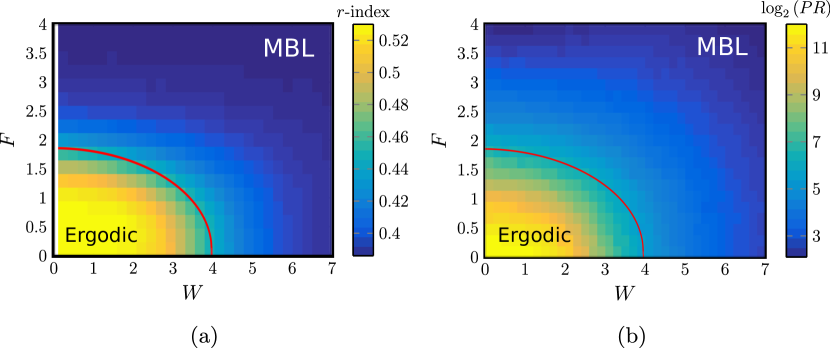
In this work we show that single-particle-localization that is not necessarily due to disorder, results in a state that is indistinguishable from the MBL state based on the typical tools of assessment. We analyze the spectral and the dynamical properties of one-dimensional interacting fermions and spins in the presence of both disorder and a linear potential. We show that by considering these two different localizing mechanisms, i.e., disorder () and linear fields (), one may construct a two-dimensional phase diagram in the -space which hosts a connected non-ergodic (MBL) phase. We find that above a critical value , the MBL phase extends down to the clean limit, i.e., the line.
It is worth mentioning that integrable models, such as the D Heisenberg and transverse field Ising models, are known examples of clean models that fail to thermalize. While these models fail to thermalize, they are sensitive to the existence of small integrability-breaking terms such as disorder or longer range interactions and hopping. In this sense the model we suggest is more generic, since the addition of disorder and/or weak longer range hopping and interactions does not lead to thermalization.
The existence of generic clean models that fail to thermalize may have important implications both theoretically and experimentally. From the theory side, it can simplify dramatically the numerical effort in analyzing these interacting systems. Moreover, the lack of randomness gives hope that the nature of the MBL transition, the emergent conserved quantities and the generalization to higher dimensions may be approached analytically. From the experimental side the necessity of strong disorder is a major drawback. In intrinsic systems it is not clear whether such strong disorder generically exists. In controlled systems, such as optical lattices, only quasi-random disorder or correlated disorder, e.g. speckle potentials, may be implemented and a repetition over many realizations is needed due to the small size of the systems Garreau (2017); Sanchez-Palencia et al. (2007). In stark contrast, linear field (tilt in optical lattices) may be implemented relatively easily and it provides the ability to experimentally realize these systems in a highly reproducible way, and without the necessity of many repetitions. Unlike integrable models, the inevitable existence of unwanted terms such as weak disorder, should not have a dramatic effect on the dynamics.
II Background and Model Definition
II.1 Bloch localization
Our ultimate goal is to understand the fate of Bloch localization in the presence of interactions. In this section we briefly review the properties of non-interacting particles in the presence of a uniform force (linear potential). Consider a D lattice model in the presence of a linear potential,
| (1) |
where annihilates a particle from lattice site , is the nearest neighbor hopping amplitude, and is the uniform force. The Hamiltonian can be diagonalized by the following transformation,
| (2) |
with being the Bessel functions of the first kind and . Under this transformation Eq. (1) becomes,
| (3) |
Since for , all the eigenstates are localized for any . Each eigenstate, , is localized around site with an inverse localization length given by .
Unlike for Anderson localization, where the localization length is energy dependent (smaller near the middle of the energy band), for Bloch localization case the localization length is an energy independent quantity. Another prominent difference between the two is the form of the density of states, where in the case of Bloch localization the spectrum forms an ordered ladder even deep in the localized phase.
II.2 Model Definition
The basic model we wish to analyze concerns the interplay between the two mechanisms of single particle localization (disorder and linear field) and interactions. For that, we consider a D lattice of interacting spinless fermions in the presence of disorder and a uniform force,
| (4) |
where annihilates a particle from lattice site , is the density, is the nearest-neighbor (nn) hopping amplitude, is the uniform force, is a random on-site potential with strength and is the nn interaction strength.
The above fermionic Hamiltonian may be mapped, via a Jordan-Wigner transformation, into an equivalent spin- chain (Heisenberg),
| (5) |
with and while and defined as before. In the rest of this paper we will analyze the localization and dynamical properties of these Hamiltonians as a function of the interaction strength, force and disorder strength. Since the particle-number (fermionic model) or the total (spin model) are conserved, we focus our analysis on the half-filled () sector. Regardless, the results do not depend much on the specific sector.
III Results and Discussion
III.1 Level statistics
A well established signature for the transition from ergodic to non-ergodic dynamics is the level statistics of the many body spectrum. In particular, generic ergodic Hamiltonians belong to the Gaussian Orthogonal Ensemble (GOE) Guhr et al. (1998); Olshanii et al. (2012) and their level-spacings, , typically obey the Wigner-Dyson distribution. On the other hand, for non-ergodic systems the level-spacings typically obey the Poisson distribution. It should be pointed out that in both cases, symmetries may add high level of degeneracies which lead to deviation from the Wigner-Dyson distribution (non-ergodic) and from perfect Poisson distribution (ergodic). Yet, level spacing obtained from symmetry sectors should not have these additional degeneracies. As in the case of the disordered Heisenberg chain within the sector of zero total magnetization, the transition from ergodic to non-ergodic is accompanied by a transition from Wigner-Dyson to Poisson level statistics Pal and Huse (2010).
Both distributions are often characterized by a single parameter, , which conveniently avoids the need for unfolding the spectrum. For the Wigner-Dyson distribution and for the Poisson distribution.
We diagonalize the Hamiltonian in Eq. (5) for spins using exact diagonalization, with and for different values of and . In the appendices we show that by employing machine learning techniques, statistics for the -value may be generated from directly without the need of diagonalizing the Hamiltonian.
In Fig. 1(a) we show the value (averaged over different disorder realizations) in the space of . We find that the ergodic phase lives in a dome-shaped region near the origin of the space. The line corresponds to the often discussed MBL transition near the critical disorder strength . As increases, the value of decreases. Above a critical value of , the critical disorder appears to go to zero and the non-ergodic phase appears also in the clean non-disordered limit.
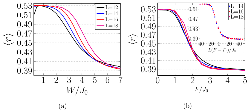
In Fig. 2 we show the value for different system sizes as a function disorder (zero field) and as a function of the field (for a fixed weak disorder). The critical values may be extracted by finite size scaling through a scaling collapse. The case of zero field was analyzed in several works Oganesyan and Huse (2007); Luitz et al. (2015); Bertrand and García-García (2016); Kudo and Deguchi (2018) in which the critical disorder was found to be in the range (notice a factor of due to a different definition of the spin matrices). For the weak disorder case we plot the data, Fig. 2 (inset), as a function of . We find that the critical exponent is and the critical field is , for which the data collapse on one curve. In the appendices we provide more details regarding the finite size scaling, and show that the above results are not sensitive to integrability-breaking terms such as next-next-nearest-neighbor hopping and interactions.
Notice that in this part, we always considered , since for small enough disorder, small systems behave as clean systems which leads to symmetry related degeneracies in the spectrum.
III.2 Inverse participation ratio
Analyzing level statistics of clean systems requires a separation of the Hilbert space into momentum sectors, since degeneracies due to symmetries have to be removed. For finite systems and below a critical disorder strength, the system behaves similar to a clean system. Therefore, the level statistics becomes a less reliable measure for small disorder strengths since degeneracies start to appear due to the emergence of translation symmetry. A quantity which is less sensitive to symmetries is the inverse participation ratio (IPR). The IPR is also a measure of the long-time return probability of arbitrary initial states. To see that, consider the return probability of a state ,
| (6) |
where is the time evolution operator. The state may be expanded in terms of the Hamiltonian eigenstates, which allows to write the IPR (long-time limit of the return probability) as,
| (7) |
In the absence of degeneracies, Eq. (7) becomes . Clearly, if the initial state is an eigenstate then , while if the initial states is an equal-superposition of all the eigenstates then , where is the Hilbert space dimension which generically is exponential in the system size. In the following we average the over different initial states which we choose to be eigenstates of some local operators, e.g., . For ergodic systems, the should be exponentially small in the system size and the system should lose its memory of the initial state. In stark contrast, in the localized phase the converges to a positive system size independent constant.
In Fig. 1(a) we present the averaged and normalized participation ratio, , in the space of . While the IPR is a smooth function, there is a transition between a region where the IPR is exponentially small to a region where the IPR is independent of system size. These regions agree with the results obtained in the previous section. Here also the line behaves in a similar way (c.f. Fig. 1(b)), where the IPR becomes independent of system size as a function of .
III.3 Dynamics and experimental measurables
The distinction between ergodic and non-ergodic dynamics is well-captured by the level-statistics and the participation ratio. Yet both these measures are hard to access in experiments. As shown in Refs. Choi et al. (2016); Schreiber et al. (2015); Bordia et al. (2017), the nature of the dynamics is examined by tracking the dynamics of an initially prepared out-of-equilibrium density configuration. We numerically show that the existence of a linear field prevents thermalization. For concreteness, we consider a similar out-of-equilibrium initial state as in Ref. Choi et al. (2016).
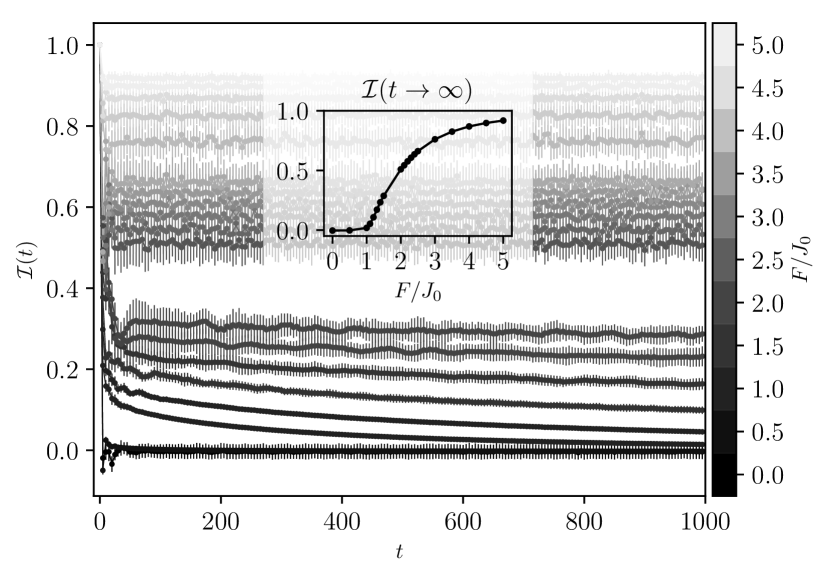
The system is prepared in a anti-ferromagnetic configuration (or charge density wave for the fermions), where the spins on odd sites point down (empty) and on even sites point up (full). We then track the time evolution of the odd-even imbalance, . We use a numerical method based on Krylov-subspaces via a re-orthogonalized Lanczos implementation to do so (see the appendices for more information).
In the inset of Fig. 3 we show the resulting long time limit as a function of . Below a critical value the long time limit of tends to zero, while above that value the long time limit tends to a finite value that increases with the field. Computational costs limit the available times we can access, and we remark that not each of these curves have converged yet. Extrapolating the available curves will move the estimated critical field to higher values than suggested by the inset.
In ergodic systems, is expected to decay to zero with a typical relaxation time . We show that while indeed this is the case when the linear field is small, both for the clean case and for weak disorder, beyond a critical field strength, the long time limit of is different from zero. In Fig. 3 we show the imbalance in a system of spins (sites) as a function of time for different values of the field and for a fixed weak disorder strength (). It is worth noticing that energetics gives an upper bound to this relaxation process. In the fermionic language, the charge density wave (CDW) configuration and the uniform configuration differ in their dipole moment by an extensive amount . In the absence of a field, the many-body bandwidth of the Heisenberg model with all is . Hence, in the presence of a field, if or the CDW configuration can not evolve into a uniform configuration at any time. In practice, the critical field obtained from the the level statistics is around while it seems that the dynamics suggests a slightly lower value (notice that not all of the imbalance curves have converged yet). Yet, while the the true critical field (if it exists) should limit the dynamics of all processes, specific processes like the one considered here may show non-ergodic dynamics at lower values. Moreover, one may consider the presence of a pre-localized phase (or pre-thermal for that matter) that appears in the dynamics. Our numerical data cannot confirm or disprove the existence of such a phase. An analysis of larger systems, and more importantly, much longer times, may resolve that issue.
IV MBL in two-dimensions
The lesson we learned about the effect of interaction on the Anderson localized (AL) phase in D can not be trivially extended to higher dimensions. The nature, and even the existence, of a many-body-localized phase in is a hotly debated subject. While theoretical works Chandran et al. (2016); De Roeck and Huveneers (2017); De Roeck and Imbrie (2017) showed that locally thermal regions in systems with true random disorder can destabilize the MBL phase in two dimensions, experimental works Choi et al. (2016); Kondov et al. (2015); Bordia et al. (2017) have shown indications for such a phase in .
Similar questions may be posed in the context of the uniform field as a cause for single particle localization. In stark contrast to the AL phase, this phase is not sensitive to rare regions. In particular, if the field is applied at an irrational angle, the field is non-zero along all lattice directions. This field can indeed be arbitrarily small for specific lattice directions, but can be chosen such that lattice sites along directions at which the field is below the critical value are separated by multiple hops. Since each of these hopping processes has a component against a strong field, and since the bare interaction is local, both the effective hopping coefficient and the effective interaction along these directions may be extremely small. How these renormalized hopping coefficients and interactions scale with the field along these direction, and whether it is possible to choose the field such that along each lattice direction the field is larger than the D critical field, is an interesting question worth further investigation. Additionally, along these same lattice directions the linear potential is not perfect and can be regarded as a combination of a linear field and weak quasi-periodic disorder. This quasi-periodic disorder may also help the localization along directions where the field is small. Finally, the absence of rare regions (which are a main reason to exclude MBL in high dimensions De Roeck and Huveneers (2017)) may help the survival of the non-ergodic behavior in the thermodynamic limit.
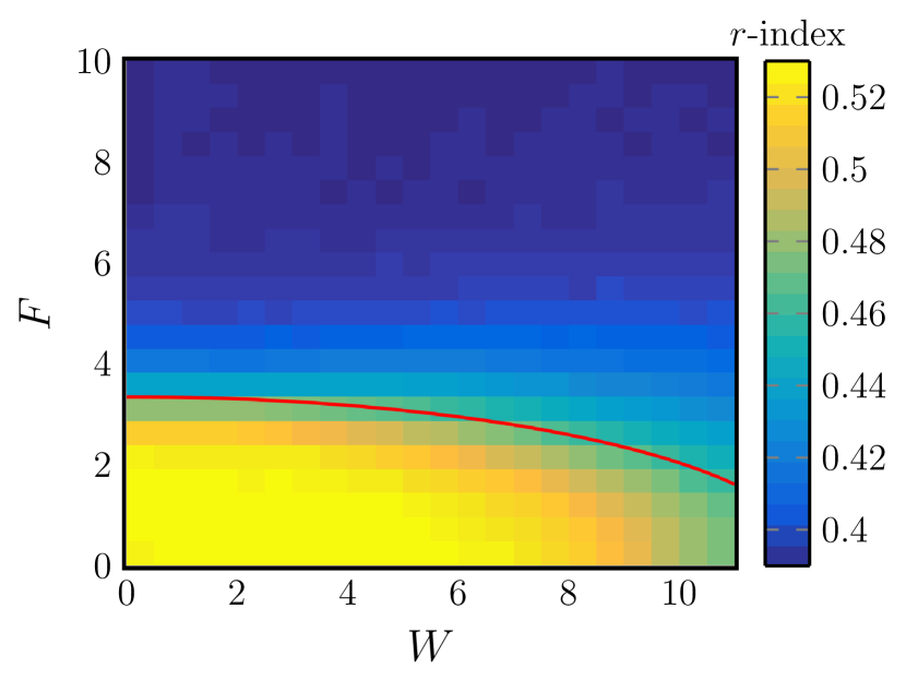
To further speculate on the existence of MBL in 2D, Fig. 4 shows the level statistics (r index) of a D Heisenberg model as a function of the uniform force and disorder. Similar to the D case, we see a clear transition from a Wigner-Dyson distribution to Poisson distribution. Since we are restricted to very small system sizes ( lattice), these results should not be taken as a claim of the existence of a two dimensional MBL phase. However, we hope that these ideas will stimulate further works in this directions.
V Dipole moment analysis
Single-particle Wannier-Stark localization may be thought of in terms of energetic constraints imposed by the field. In the many-body case, one may wonder whether interactions can help overcome energetic constraints by reordering of particles. Heuristically, a many-body configuration can be described by its dipole moment (see section III.3), which in the presence of a field is associated with an energy . In order for such a configuration to evolve into a different configuration with dipole moment , the internal structure of the system, i.e., hopping and interaction, must be able to supply the energy difference . This condition is captured in the dipole moment structure of the eigenstates. Clearly, in the infinite field limit of our model, the dipole moment becomes an exactly conserved quantity. In that case an analogy with Ref. Pai et al. (2018) can be made, where it was shown that non-ergodic dynamics arises in a one dimensional random quantum circuit model which is constrained to conserve both a charge and the dipole moment of this charge.
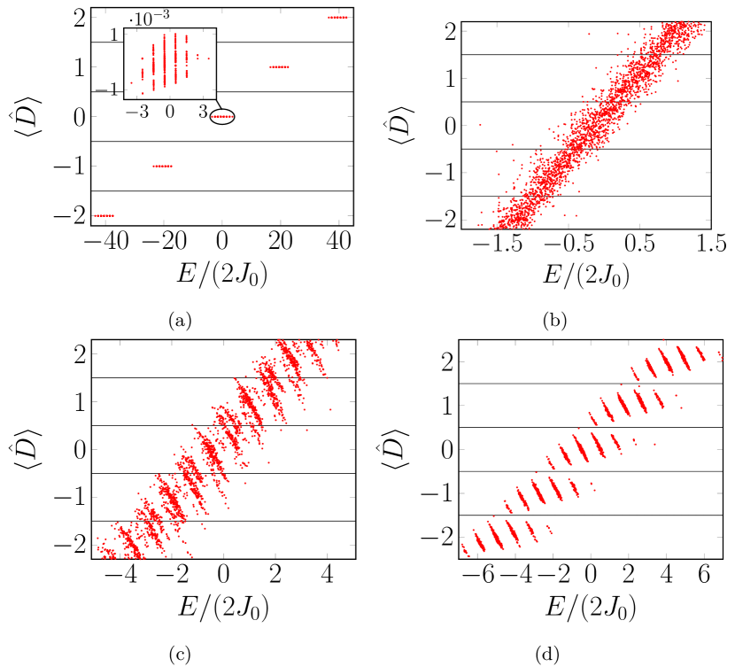
The main question is to what extent the dipole moment may be considered as a conserved quantity for finite fields. In the appendices we show the results of exact diagonalization of a half-filled fermionic system where each point represents an eigenstate in the space of energy and dipole-moment. As expected, in a given energy window and for large field the many body wave functions have well-defined dipole moment. Each dipole moment sector is further split into subsectors of doublon (occupied neighboring sites) number. Hence the dynamics is effectively restricted to preserve the initial dipole moment and the initial doublon number, which is predicted to yield non-ergodic dynamics Pai et al. (2018). For a weak field however, this is not the case. The eigenstates in a given energy window span a range of dipole moments and doublon numbers. Around the critical field, we observe that while the eigenstates in a given energy have a finite spread in the dipole moment, the different sectors become distinct and the integer part of the dipole moment behaves as a conserved quantity. Beyond this critical field we also observe a separation into the subsectors of doublon number. While it is hard to pinpoint the exact value of the transition using this approach, the transition can be bounded and is consistent with the value we obtained from the level spacing statistics.
VI Conclusions
In this work we analyzed the effect of interactions on single particle localization that arise both from disorder, , and from the existence of linear potentials . With that, we showed that the notion of a many-body localized (MBL) phase may be generalized also to a class of clean (non-integrable) systems. In particular, we find that a phase boundary in the space exists, beyond which the resulting phase fails to thermalize. We find that, unlike in clean integrable models, this non-ergodic phase is stable to perturbations, and shares all the familiar fingerprints of the well studied MBL phase in the presence of disorder.
The existence of such a phase demonstrates that randomness is not an essential ingredient for the emergence of stable non-ergodic interacting phases. Such a conclusion may have an impact on the realization of these non-ergodic phases. Unlike disorder potentials, linear potentials are relatively easy to implement, and are highly tunable and may be controlled dynamically. The ability to realize stable and generic non-ergodic phases is an important step toward the realization of quantum memory devices that may store information for long times. Moreover, the lack of randomness and the low sensitivity to dimensionality may render these systems more accessible to a further theoretical investigation, both numerically and analytically. It came to our knowledge that simultaneously to our work, the entanglement-entropy grows in the presence of linear field has been studied in Refs. Schulz et al. (2018). The results presented in Refs. Schulz et al. (2018) are in agreement with the conclusions we presented in this work.
Acknowledgements.
E.v.N. gratefully acknowledges financial support from the Swiss National Science Foundation through grant P2EZP2-172185. G.R. is grateful to the ARO MURI W911NF-16-1-0361 “Quantum Materials by Design with Electromagnetic Excitation” sponsored by the U.S. Army as well as the Packard Foundation. We are grateful for support from the IQIM, an NSF physics frontier center funded in part by the Moore Foundation.The C++ code we developed for this is available online at https://www.github.com/everthemore/krylov-cpp, and the data for Fig. 3 is available at https://data.caltech.edu/records/1089.
Appendix A Data augmentation using machine learning
The different disorder realizations we study in this manuscript differ only in the values for the on-site potentials. Given the on-site potentials, there exists a procedure that results in the value for the -statistics. Namely, one builds the corresponding Hamiltonian matrix and diagonalizes it to obtain the eigenvalues . The r-statistics is obtained by looking at neighboring eigenvalue differences and computing the ratio as discussed in the main text.
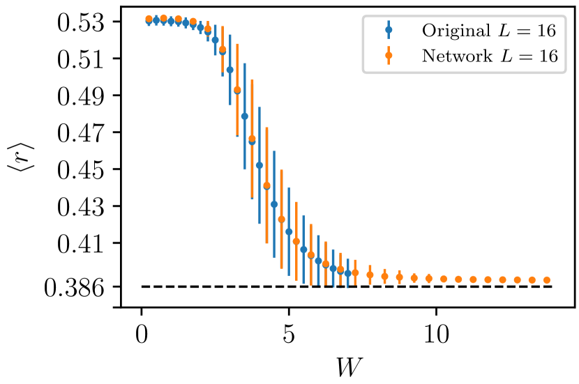
Here, however, we ask whether or not a more direct (approximate) map exists from the on-site potentials to . Rather than trying to explicitly construct it, we attempt to train a neural network to perform this map for us. Hence we generate a large data-set of pairs , where is a vector of the on-site potentials augmented with the value of from which they were drawn, and is the resulting -statistics for this particular realization. These serve as the input and output respectively for the machine learning model.
Provided that such a mapping exists and that the network is capable of learning it, the resulting network can be used to generate more -values by using it to predict on more realizations. This allows one to generate statistics much faster compared to running the full exact diagonalization. It must be noted that this procedure cannot take away the inherent statistical uncertainty due to the finite size of the system. Particularly, for disorder strengths near the transitions point, the exact -values of systems with different realizations drawn from the same distribution, lie within a relatively large window. As the system becomes larger this window becomes smaller. For example, already by including a few hundreds of realizations, for , the error bars near the transition are dominated by the intrinsic finite size effect and cannot be improved by adding more realizations.
In Fig. 5 we demonstrate the above procedure for the data, for which the data-set consists of k entries ( values of spread over realizations). We split off of the data as a validation set, and train a network with the following architecture. First, two convolutional layers with filters and kernel sizes and , followed by a maximum pooling of size 3. Then a convolutional layer with 64 filters and kernel size 2, followed by a global average pooling. Next, two fully connected sigmoid layers with 256 and 128 neurons respectively, and dropout 0.5. And finally an output layer with a single sigmoid neuron.
We train the network with the Adam Kingma and Ba (2014) optimizer to minimize the mean-squared-error loss function, and achieve a validation loss of in 100 epochs of batchsize . In our experiments, we have found no particular reason for the above network to work better than others, but we found that considerably simpler networks (e.g. just fully connected layers) converge much slower. For the purpose of extracting the mapping, our chosen network might be hard to interpret. It would be an interesting research direction however to see if the approximate mapping can be extracted from a network, or whether a single network can be trained on different system sizes to extract finite size behavior. Both would potentially allow predictions to be made on larger system sizes than trained on, although further investigation into this question is required.
Finite size scaling
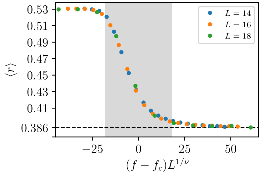
In this appendix we discuss the transition from the ergodic to the non-ergodic phase as a function of the linear field . To do so, we fix and perform a finite size scaling analysis attempting to collapse the curves for different system sizes. We consider a universal function for the -statistics, and optimize the parameters and so that the rescaled -statistics curves for the different sizes collapse.
Each of the curves is first rescaled with proposed and after which we use spline interpolation to numerically minimize the cost function , where both run over system sizes and represents the spline-interpolated data. The integration regime is taken to be centered around the transition (i.e. ) and has a width that we vary to obtain statistics on and . In the collapse including the system size data, the curve is consistently the most off. In the spirit of Ref. Luitz et al. (2015) we consider the width for which the extracted parameters are least sensitive to the inclusion/removal of the data. This results in the parameters and . The resulting collapse for this set of parameters is shown in Fig. 6.
Appendix B Choice of gauge for numerics
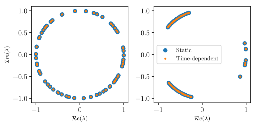
We chose to work with a time-independent Hamiltonian for which the linear field is added via the dipole term, rather than as a time-dependent phase factor for the hopping. This interpretation brings with it the potential issue of having an infinite energy difference between the endpoints of our system as one scales up to the thermodynamic limit. The physics in these two gauges is evidently invariant, but since we consider (rather small) finite size systems the infinite energies are not a concern. Working in the time-independent gauge is numerically considerably more convenient, since the time evolution operator over a period , i.e. , can be constructed by a single exponentiation through as . For the time-dependent case, one would have to compute the time ordered integral by breaking it down into many small -sized steps and exponentiating for each. The resulting differences in the spectra and are only of the order of . An interesting phenomenon for future investigation is the observed clustering of the eigenvalues for field , shown in Fig. 7.
Appendix C Sensitivity to integrability-breaking terms
We now consider an extended version of Eq. 5 of the main text,
| (8) | ||||
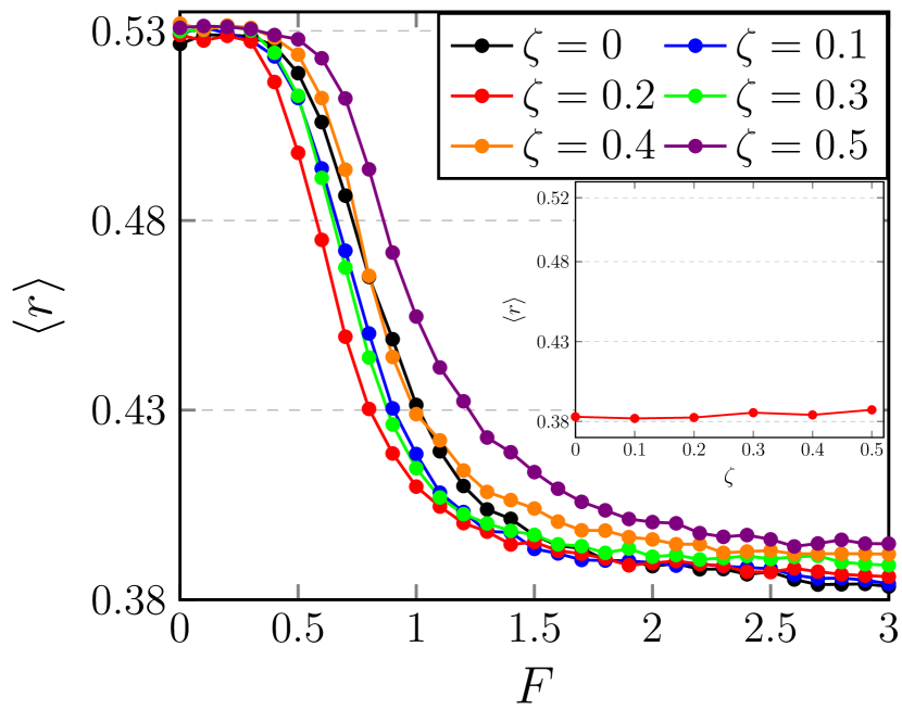
In the absence of both disorder and linear field, the above model is integrable for . We show that also in the presence of the integrability-breaking terms, the application of linear field (with or without disorder) leads to a transition from a Wigner-Dyson level statistics (ergodic) to a Poisson level statistics (non-ergodic). While the value of the critical field depends on and the disorder strength, the qualitative behavior is indifferent to these terms. In Fig. 8 we show the -index as a function of the linear field strength. Different curves represent different values of .
Appendix D Time-evolution using the re-orthogonalized Lanczos algorithm
In this appendix we discuss algorithmic details of simulating the time-evolution of a wavefunction using a Krylov-subspace method. In particular, we have used the so-called Lanzcos algorithm with re-orthogonalization to obtain the results presented in Fig. 3 of the main text.
We wish to numerically perform the time-evolution of a wavefunction, i.e., to compute . To do this exactly would require the full diagonalization of the Hamiltonian , which becomes impossible for large system sizes due to memory requirements. An improvement can be made by using a sparse matrix implementation of the Hamiltonian and iteratively simulating
| (9) |
for small time-steps . A naive implementation of this iterative algorithm quickly accumulates numerical errors and becomes unstable, however, a more stable variant can be constructed using Krylov-subspaces Moler and Van Loan (2003). A Krylov-subspace of dimension , , is defined as the span of the vectors . The vector , after expanding the exponent on right-hand side of Eq. 9, is approximated well by a vector in this Krylov subspace.
The vectors in first need to be orthonormalized (discussed in more depth shortly), after which we store them as the columns of a new matrix of dimension , where is the size of the Hilbert space. After obtaining , we project the Hamiltonian into the spanned subspace to obtain . This is a much smaller matrix that can be easily exponentiate, and allows us to compute
| (10) |
In all of the above, the Krylov subspace dimension can either be systematically increased until convergence is obtained, or changed adaptively during the orthogonalization procedure described next.
The numerically most challenging step in this algorithm is obtaining the orthonormalized set of vectors for from . A standard Gram-Schmidt procedure for orthonormalizing a set of vectors loses the orthogonality between successive vectors simply due to rounding errors (i.e. finite precision of floating point numbers). The modified Gram-Schmidt procedure does considerably better, but we have found it insufficient for our purpose. The set of vectors we wish to orthonormalize is a special set, in which each vector is generated from the previous one by application of a matrix. This means we can generate the vectors during the Gram-Schmidt procedure instead of having them given to use beforehand. This small but important difference leads to this algorithm often being called the Arnoldi method. The resulting projected matrix is in general an upper Hessenberg matrix (upper triangular plus the first lower off-diagonal). If the matrix is Hermitian as it is in our case, the projected matrix is therefore tri-diagonal. The Arnoldi algorithm with a Hermitian matrix is called the Lanczos algorithm, and provides an improvement in terms of computational effort.
Regardless of using modified Gram-Schmidt, Arnoldi or Lanczos, the orthogonality between successive vectors is gradually lost. A significant improvement, at computational cost of course, can be made by simply re-orthogonalizing the set of obtained (semi-)orthogonal vectors. It turns out that for the re-orthogonalization “twice is enough” for non-singular cases Giraud et al. (2005). For the numerics presented in Fig. 3 of the main text, we have checked the convergence of the curves with respect to the timestep dt and the Krylov-subspace dimension . The values we have used are and .
Appendix E Dipole moment analysis
We show in Fig. 9 the results of exact diagonalization of a half-filled fermionic system where each point represents an eigenstate in the space of energy and dipole-moment. As expected, in a given energy window and for large field (Fig. 9a) the many body wave functions have well-defined dipole moment. For a weak field however (Fig. 9b), this is not the case. The eigenstates in a given energy window span a range of dipole moments. Around the critical field (Fig. 9c,d), while the eigenstates in a given energy have a finite spread in the dipole moment, the different sectors become distinct and the integer part of the dipole moment behaves as a conserved quantity.
References
- Anderson (1958) P. W. Anderson, “Absence of diffusion in certain random lattices,” Phys. Rev. 109, 1492–1505 (1958).
- Basko et al. (2006) D.M. Basko, I.L. Aleiner, and B.L. Altshuler, “Metal–insulator transition in a weakly interacting many-electron system with localized single-particle states,” Annals of Physics 321, 1126 – 1205 (2006).
- Gornyi et al. (2005) I. V. Gornyi, A. D. Mirlin, and D. G. Polyakov, “Interacting electrons in disordered wires: Anderson localization and low- transport,” Phys. Rev. Lett. 95, 206603 (2005).
- Nandkishore and Huse (2015) Rahul Nandkishore and David A. Huse, “Many-body localization and thermalization in quantum statistical mechanics,” Annual Review of Condensed Matter Physics 6, 15–38 (2015).
- Abanin and Papić (2017) Dmitry A. Abanin and Zlatko Papić, “Recent progress in many-body localization,” Annalen der Physik 529, 1700169–n/a (2017), 1700169.
- Imbrie (2016) John Z. Imbrie, “Diagonalization and many-body localization for a disordered quantum spin chain,” Phys. Rev. Lett. 117, 027201 (2016).
- Huse et al. (2014) David A. Huse, Rahul Nandkishore, and Vadim Oganesyan, “Phenomenology of fully many-body-localized systems,” Phys. Rev. B 90, 174202 (2014).
- Oganesyan and Huse (2007) Vadim Oganesyan and David A. Huse, “Localization of interacting fermions at high temperature,” Phys. Rev. B 75, 155111 (2007).
- Pal and Huse (2010) Arijeet Pal and David A. Huse, “Many-body localization phase transition,” Phys. Rev. B 82, 174411 (2010).
- Vosk et al. (2015) Ronen Vosk, David A. Huse, and Ehud Altman, “Theory of the many-body localization transition in one-dimensional systems,” Phys. Rev. X 5, 031032 (2015).
- Bar Lev and Reichman (2014) Yevgeny Bar Lev and David R. Reichman, “Dynamics of many-body localization,” Phys. Rev. B 89, 220201 (2014).
- White et al. (2018) Christopher David White, Michael Zaletel, Roger S. K. Mong, and Gil Refael, “Quantum dynamics of thermalizing systems,” Phys. Rev. B 97, 035127 (2018).
- van Nieuwenburg et al. (2017) E. van Nieuwenburg, E. Bairey, and G. Refael, “Learning phase transitions from dynamics,” ArXiv e-prints (2017), arXiv:1712.00450 [cond-mat.dis-nn] .
- Bauer and Nayak (2013) Bela Bauer and Chetan Nayak, “Area laws in a many-body localized state and its implications for topological order,” Journal of Statistical Mechanics: Theory and Experiment 2013, P09005 (2013).
- Žnidarič et al. (2008) Marko Žnidarič, Toma ž Prosen, and Peter Prelovšek, “Many-body localization in the heisenberg magnet in a random field,” Phys. Rev. B 77, 064426 (2008).
- Bardarson et al. (2012) Jens H. Bardarson, Frank Pollmann, and Joel E. Moore, “Unbounded growth of entanglement in models of many-body localization,” Phys. Rev. Lett. 109, 017202 (2012).
- Khemani et al. (2017a) Vedika Khemani, S. P. Lim, D. N. Sheng, and David A. Huse, “Critical properties of the many-body localization transition,” Phys. Rev. X 7, 021013 (2017a).
- Gopalakrishnan et al. (2015) Sarang Gopalakrishnan, Markus Müller, Vedika Khemani, Michael Knap, Eugene Demler, and David A. Huse, “Low-frequency conductivity in many-body localized systems,” Phys. Rev. B 92, 104202 (2015).
- Berkelbach and Reichman (2010) Timothy C. Berkelbach and David R. Reichman, “Conductivity of disordered quantum lattice models at infinite temperature: Many-body localization,” Phys. Rev. B 81, 224429 (2010).
- Lazarides et al. (2015) Achilleas Lazarides, Arnab Das, and Roderich Moessner, “Fate of many-body localization under periodic driving,” Phys. Rev. Lett. 115, 030402 (2015).
- D’Alessio and Polkovnikov (2013) Luca D’Alessio and Anatoli Polkovnikov, “Many-body energy localization transition in periodically driven systems,” Annals of Physics 333, 19 – 33 (2013).
- Khemani et al. (2016) Vedika Khemani, Achilleas Lazarides, Roderich Moessner, and S. L. Sondhi, “Phase structure of driven quantum systems,” Phys. Rev. Lett. 116, 250401 (2016).
- Smith et al. (2016) J. Smith, A. Lee, P. Richerme, B. Neyenhuis, P. W. Hess, P. Hauke, M. Heyl, D. A. Huse, and C. Monroe, “Many-body localization in a quantum simulator with programmable random disorder,” Nature Phys. 12 (2016), 10.1038/nphys3783.
- Choi et al. (2016) Jae-yoon Choi, Sebastian Hild, Johannes Zeiher, Peter Schauß, Antonio Rubio-Abadal, Tarik Yefsah, Vedika Khemani, David A. Huse, Immanuel Bloch, and Christian Gross, “Exploring the many-body localization transition in two dimensions,” Science 352, 1547–1552 (2016).
- Schreiber et al. (2015) Michael Schreiber, Sean S. Hodgman, Pranjal Bordia, Henrik P. Lüschen, Mark H. Fischer, Ronen Vosk, Ehud Altman, Ulrich Schneider, and Immanuel Bloch, “Observation of many-body localization of interacting fermions in a quasirandom optical lattice,” Science 349, 842–845 (2015).
- Kondov et al. (2015) S. S. Kondov, W. R. McGehee, W. Xu, and B. DeMarco, “Disorder-induced localization in a strongly correlated atomic hubbard gas,” Phys. Rev. Lett. 114, 083002 (2015).
- Bordia et al. (2017) Pranjal Bordia, Henrik Lüschen, Sebastian Scherg, Sarang Gopalakrishnan, Michael Knap, Ulrich Schneider, and Immanuel Bloch, “Probing slow relaxation and many-body localization in two-dimensional quasiperiodic systems,” Phys. Rev. X 7, 041047 (2017).
- De Roeck et al. (2016) Wojciech De Roeck, Francois Huveneers, Markus Müller, and Mauro Schiulaz, “Absence of many-body mobility edges,” Phys. Rev. B 93, 014203 (2016).
- Smith et al. (2017a) A. Smith, J. Knolle, D. L. Kovrizhin, and R. Moessner, “Disorder-free localization,” Phys. Rev. Lett. 118, 266601 (2017a).
- Smith et al. (2017b) A. Smith, J. Knolle, R. Moessner, and D. L. Kovrizhin, “Absence of ergodicity without quenched disorder: From quantum disentangled liquids to many-body localization,” Phys. Rev. Lett. 119, 176601 (2017b).
- Smith et al. (2018) Adam Smith, Johannes Knolle, Roderich Moessner, and Dmitry L. Kovrizhin, “Dynamical localization in lattice gauge theories,” Phys. Rev. B 97, 245137 (2018).
- Grover and Fisher (2014) Tarun Grover and Matthew P A Fisher, “Quantum disentangled liquids,” Journal of Statistical Mechanics: Theory and Experiment 2014, P10010 (2014).
- Kagan and Maksimov (1984) Yu. Kagan and L.A. Maksimov, “Localization in a system of interacting particles diffusing in a regular crystal,” JETP 60, 201 (1984).
- De Roeck and Huveneers (2014) Wojciech De Roeck and Fran çois Huveneers, “Scenario for delocalization in translation-invariant systems,” Phys. Rev. B 90, 165137 (2014).
- Schiulaz et al. (2015) Mauro Schiulaz, Alessandro Silva, and Markus Müller, “Dynamics in many-body localized quantum systems without disorder,” Phys. Rev. B 91, 184202 (2015).
- Yao et al. (2016) N. Y. Yao, C. R. Laumann, J. I. Cirac, M. D. Lukin, and J. E. Moore, “Quasi-many-body localization in translation-invariant systems,” Phys. Rev. Lett. 117, 240601 (2016).
- Iyer et al. (2013) Shankar Iyer, Vadim Oganesyan, Gil Refael, and David A. Huse, “Many-body localization in a quasiperiodic system,” Phys. Rev. B 87, 134202 (2013).
- Lüschen et al. (2017) Henrik P. Lüschen, Pranjal Bordia, Sebastian Scherg, Fabien Alet, Ehud Altman, Ulrich Schneider, and Immanuel Bloch, “Observation of slow dynamics near the many-body localization transition in one-dimensional quasiperiodic systems,” Phys. Rev. Lett. 119, 260401 (2017).
- Khemani et al. (2017b) Vedika Khemani, D. N. Sheng, and David A. Huse, “Two universality classes for the many-body localization transition,” Phys. Rev. Lett. 119, 075702 (2017b).
- Kim and Haah (2016) Isaac H. Kim and Jeongwan Haah, “Localization from superselection rules in translationally invariant systems,” Phys. Rev. Lett. 116, 027202 (2016).
- Wannier (1960) Gregory H. Wannier, “Wave functions and effective hamiltonian for bloch electrons in an electric field,” Phys. Rev. 117, 432–439 (1960).
- G. et al. (1979) Casati G., Chirikov B.V., Izraelev, and F.M. Ford J., “Stochastic behavior of a quantum pendulum under a periodic perturbation,” Casati G., Ford J. (eds) Stochastic Behavior in Classical and Quantum Hamiltonian Systems. Lecture Notes in Physics, vol 93. Springer, Berlin, Heidelberg 93 (1979).
- Baum et al. (2018) Yuval Baum, Evert P. L. van Nieuwenburg, and Gil Refael, “From dynamical localization to bunching in interacting floquet systems,” SciPost Phys. 5, 17 (2018).
- Luitz et al. (2017) David J. Luitz, Yevgeny Bar Lev, and Achilleas Lazarides, “Absence of dynamical localization in interacting driven systems,” SciPost Phys. 3, 029 (2017).
- Eckstein and Werner (2011) Martin Eckstein and Philipp Werner, “Damping of bloch oscillations in the hubbard model,” Phys. Rev. Lett. 107, 186406 (2011).
- Krimer et al. (2009) Dmitry O. Krimer, Ramaz Khomeriki, and Sergej Flach, “Delocalization and spreading in a nonlinear stark ladder,” Phys. Rev. E 80, 036201 (2009).
- Pieri and Strinati (2003) P. Pieri and G. C. Strinati, “Derivation of the gross-pitaevskii equation for condensed bosons from the bogoliubov˘de gennes equations for superfluid fermions,” Phys. Rev. Lett. 91, 030401 (2003).
- Garreau (2017) Jean-Claude Garreau, “Quantum simulation of disordered systems with cold atoms,” Comptes Rendus Physique 18, 31 – 46 (2017), prizes of the French Academy of Sciences 2015 / Prix de l’Académie des sciences 2015.
- Sanchez-Palencia et al. (2007) L. Sanchez-Palencia, D. Clément, P. Lugan, P. Bouyer, G. V. Shlyapnikov, and A. Aspect, “Anderson localization of expanding bose-einstein condensates in random potentials,” Phys. Rev. Lett. 98, 210401 (2007).
- Guhr et al. (1998) Thomas Guhr, Axel Müller–Groeling, and Hans A. Weidenmüller, “Random-matrix theories in quantum physics: common concepts,” Physics Reports 299, 189 – 425 (1998).
- Olshanii et al. (2012) Maxim Olshanii, Kurt Jacobs, Marcos Rigol, Vanja Dunjko, Harry Kennard, and Vladimir A. Yurovsky, “An exactly solvable model for the integrability and chaos transition in rough quantum billiards,” Nature Communications 3 (2012), 10.1038/ncomms1653.
- Luitz et al. (2015) David J. Luitz, Nicolas Laflorencie, and Fabien Alet, “Many-body localization edge in the random-field heisenberg chain,” Phys. Rev. B 91, 081103 (2015).
- Bertrand and García-García (2016) Corentin L. Bertrand and Antonio M. García-García, “Anomalous thouless energy and critical statistics on the metallic side of the many-body localization transition,” Phys. Rev. B 94, 144201 (2016).
- Kudo and Deguchi (2018) Kazue Kudo and Tetsuo Deguchi, “Finite-size scaling with respect to interaction and disorder strength at the many-body localization transition,” Phys. Rev. B 97, 220201 (2018).
- Chandran et al. (2016) A. Chandran, A. Pal, C. R. Laumann, and A. Scardicchio, “Many-body localization beyond eigenstates in all dimensions,” Phys. Rev. B 94, 144203 (2016).
- De Roeck and Huveneers (2017) Wojciech De Roeck and Fran çois Huveneers, “Stability and instability towards delocalization in many-body localization systems,” Phys. Rev. B 95, 155129 (2017).
- De Roeck and Imbrie (2017) Wojciech De Roeck and John Z. Imbrie, “Many-body localization: stability and instability,” Philosophical Transactions of the Royal Society of London A: Mathematical, Physical and Engineering Sciences 375 (2017), 10.1098/rsta.2016.0422.
- Pai et al. (2018) Shriya Pai, Michael Pretko, and Rahul M. Nandkishore, “Localization in fractonic random circuits,” arXiv e-prints , arXiv:1807.09776 (2018), arXiv:1807.09776 [cond-mat.stat-mech] .
- Schulz et al. (2018) M. Schulz, C. A. Hooley, R. Moessner, and F. Pollmann, “Stark many-body localization,” ArXiv e-prints (2018), arXiv:1808.01250 [cond-mat.dis-nn] .
- Kingma and Ba (2014) D.P. Kingma and J. Ba, “Adam: A Method for Stochastic Optimization,” ArXiv e-prints (2014), arXiv:1412.6980 .
- Moler and Van Loan (2003) C. Moler and C. Van Loan, “Nineteen dubious ways to compute the exponential of a matrix, twenty-five years later,” SIAM Review 45, 3–49 (2003), https://doi.org/10.1137/S00361445024180 .
- Giraud et al. (2005) Luc Giraud, Julien Langou, Miroslav Rozložník, and Jasper van den Eshof, “Rounding error analysis of the classical gram-schmidt orthogonalization process,” Numerische Mathematik 101, 87–100 (2005).