Entropic Leggett-Garg inequality in neutrinos and $B(K)$ meson systems

Abstract

Entropic Leggett-Garg inequality is studied in systems like neutrinos in the context of two and three flavor neutrino oscillations and in neutral $B_{d}$, $B_{s}$ and $K$ mesons. The neutrino dynamics is described with the matter effect taken into consideration. For the decohering $B/K$ meson systems, the effect of decoherence and CP violation have also been taken into account, using the techniques of open quantum systems. Enhancement in the violation with increase in the number of measurements has been found, in consistency with findings in spin-$s$ systems. The effect of decoherence is found to bring the deficit parameter $\mathcal{D}^{[n]}$ closer to its classical value zero, as expected. The violation of entropic Leggett-Garg inequality lasts for a much longer time in $K$ meson system than in $B_{d}$ and $B_{s}$ systems.

I INTRODUCTION

There is no sharp boundary between the classical and the quantum worlds. However, physicists have developed some important notions which can shed light on the distinction of the two domains. The most profound among these notions being the uncertainty principle Heisenberg (1927). The violation of Bell inequality Bell (1964); Clauser et al. (1969) is another prominent example which reveals the nonclassical nature of correlations between spatially separated quantum systems Mermin (1993). Aspect’s experiment Aspect et al. (1982) verified for the first time the CHSH form of the Bell inequality by using pairs of spatially separated polarization-entangled photons. Since then, Bell theorem has been successfully verified in many experiments Tittel et al. (1998a, b); PhysRevLett.81.5039 ; Pan et al. (2000); Rowe et al. (2001); Salart et al. (2008); Kofler et al. ; Handsteiner et al. (2017); Rosenfeld et al. (2017).

Quantum correlations could be spatial or temporal. Among spatial quantum correlations, much attention has been devoted to entanglement Horodecki et al. (2009): entangled states are non classical and sometimes display even stronger correlations such as steering Cavalcanti and Skrzypczyk and non-locality Brunner et al. (2014). However, even unentangled states, may not have a classical description. Quantum discord Ollivier and Zurek (2001); Henderson and Vedral (2001); Adhikari and Banerjee (2012) is another important spatial quantum correlation and captures the fact that local measurements on parts of a composite system induce an overall disturbance in the state. Details of various facets of spatial quantum correlations studied on different physical systems can be seen in, for example, Aspect et al. (1981); Tittel et al. (1998c, d); PhysRevLett.81.5039 ; Banerjee et al. (2010); Chakrabarty et al. (2011); Lanyon et al. (2013); Kessel and Ermakov (2000); Laflamme et al. (2001); Blasone et al. (2009); alok2016quantum ; Banerjee et al. (2015, 2016); khushQC .

Leggett-Garg inequalities (LGIs), considered to be the temporal analogue of Bell inequalities, were constructed to understand the extrapolation of quantum theory to macroscopic systems, by assuming macro-realism and noninvasive measurability Leggett and Garg (1985). Macro-realism implies that a system with two or more distinct states available to it will be, at any time, in one of these states. Noninvasive measurability means that it is possible to determine this state without disturbing the future dynamics of the system. LGIs have been studied in various theoretical works Barbieri (2009); Avis et al. (2010); Lambert et al. (2010, 2011); Montina (2012); Emary et al. (2013); Kofler and Brukner (2013); emarydeco including, in recent times, neutrino oscillations Naikoo et al. ; Fu and Chen (2017) and neutral mesons Naikoo et al. (2018) and verified in a number of experiments Palacios-Laloy et al. (2010); Groen et al. (2013); Goggin et al. (2011); Xu et al. (2011); Dressel et al. (2011); Suzuki et al. (2012); Athalye et al. (2011); Souza et al. (2011); Katiyar et al. (2013). The Leggett-Garg string for an $n$ measurement scenario is given as

$$K_{n}=\sum\limits_{i=1}^{n}C_{i,i+1}-C_{i,n}.$$ (1)

Here, $C_{ij}=\langle\hat{A}(t_{i})\hat{A}(t_{j})\rangle$ is the two time correlation function for the operator $\hat{A}$. The assumptions of macrorealism and non-invasive measurability impose the following restrictions on $K_{n}$:

$$-n \leq K_{n}\leq n-2\qquad\qquad{\rm for}~{}n\geq 3,n~{}~{}odd;$$

$$-(n-2) \leq K_{n}\leq n-2\qquad\qquad{\rm for}~{}n\geq 4,n~{}~{}even.$$ (2)

The entropic version of Bell inequality was formulated in Braunstein and Caves (1988). Entropic formulations derive their utility from their ability to deal with any finite number of outcomes, allowing, in principle, to go beyond the standard dichotomic choice of observable Chaves and Fritz (2012); Rastegin (2014). Entropic version of the temporal counterpart of Bell inequality was developed in Morikoshi (2006). This was followed by an application of the entropic version of Leggett-Garg inequality to a spin-$s$ system in Devi et al. (2013).

In this work, we will analyze the entropic Leggett-Garg inequality for the neutrino system in the context of neutrino oscillations and for the decohering $K$ and $B$ mesons by using the formalism of open quantum systems. In Sec. (II), we provide a brief account of the entropic formulation of Leggett-Garg inequality. Section (III) is devoted to a discussion of neutrino oscillations and the entropic Leggett-Garg inequality for the neutrino system. The dynamics of $K$ and $B$ mesons using the open systems approach is spelled out in Sec. (IV) wherein we also discuss the construction of entropic Leggett-Garg inequality for the meson system. Section (V) is devoted to a discussion of the results obtained. We conclude in Sec. (VI).

II Entropic Leggett-Garg inequality

We now provide a brief review of some rudiments of information theory used in the development of the entropic Leggett-Garg inequality. We begin by considering the observable $A$ which can take discrete values denoted by $a_{i}$ at time $t_{i}$, that is, $A(t_{i})=a_{i}$. We define the joint probability of the measurement of $A$ at times $t_{i}$ and $t_{j}$ giving results $a_{i}$ and $a_{j}$, respectively, as $P(a_{i},a_{j})$. According to Bayes’s theorem the joint probability is related to the conditional probability as,

$$P(a_{i},a_{j})=P(a_{j}|a_{i})P(a_{i})=P(a_{i}|a_{j})P(a_{j}).$$ (3)

Here, $P(a_{j}|a_{i})$ is the conditional probability of obtaining the outcome $a_{j}$ at time $t_{j}$, given that $a_{i}$ was obtained at time $t_{i}$.

A classical theory can assign well defined values to all observables of the system with no reference to the measurement process. This assumption lies at the heart of Bell and Leggett-Garg inequalities, leading to bounds which may not be respected by the non-classical systems. In other words, this assumption demands a joint probability distribution,
$P(a_{i},a_{j})$, yielding information about the marginals of individual observations at time $t_{i}$. The assumption of non-invasive measurability implies that the measurement made on a system at any time does not disturb its future dynamics and hence any measurement made at a later time $t_{j}$ where $t_{j}>t_{i}$. The mathematical statement would be that the joint probabilities be expressed as a convex combination of the product of probabilities $P(a_{i}|\lambda)$, averaged over a hidden variable probability distribution $\rho(\lambda)$ Kofler and Brukner (2013, 2008); Fine (1982):

$$P(a_{1},a_{2},\dots,a_{n})=\sum\limits_{\lambda}\rho(\lambda)P(a_{1}|\lambda)P(a_{2}|\lambda)\cdots P(a_{n}|\lambda),$$ (4)

such that the following properties are satisfied

$$0\leq\rho(\lambda)\leq 1,\quad\sum\limits_{\lambda}\rho(\lambda)=1;\quad 0\leq P(a_{i}|\lambda)\leq 1,\quad\sum\limits_{\lambda}P(a_{i}|\lambda)=1.$$ (5)

One can use the conditional probability given by Eq. (3) to define the conditional entropy as

$$H[A(t_{j})|A(t_{i})]=-\sum\limits_{a_{i},a_{j}}P(a_{j}|a_{i})\log_{2}P(a_{j}|a_{i}).$$ (6)

Now using chain rule and the fact that conditioning reduces entropy Cover and Thomas (2012), one obtains Morikoshi (2006)

$$H[A(t_{N-1}),...,A(t_{0})]\leq H[A(t_{N-1})|A(t_{N-2})]+...+H[A(t_{1})|A(t_{0})]+H[A(t_{0})].$$ (7)

This temporal entropic inequality was used in Morikoshi (2006) to study the role of quantum coherence in Grover’s algorithm. Using the relation $H[A(t_{i}),A(t_{i+j})]=H[A(t_{i+j})|A(t_{i})]+H[A(t_{i})]$, one can derive the temporal analogues of the spatial entropic Bell inequalities

$$\sum\limits_{k=1}^{N-1}H[A(t_{k})|A(t_{k-1})]-H[A(t_{N-1})|A(t_{0})]\geq 0.$$ (8)

These are the entropic Leggett-Garg inequalities Devi et al. (2013). Here, $N$ denotes the number of measurements, inclusive of the preparation; the case of $N=3$ was experimentally tested in Katiyar et al. (2013).

III Neutrino oscillation

Consider an arbitrary number of $n$ orthogonal flavor eigenstates $\ket{\nu_{\alpha}}$ with $\langle\nu_{\alpha}|\nu_{\beta}\rangle=\delta_{\alpha\beta}$. These flavor states are connected to $n$ mass eigenstates by a unitary operator $U$ Bilenky et al. (1999); Gonzalez-Garcia and Maltoni (2008):

$$\ket{\nu_{\alpha}}=\sum\limits_{k}U_{\alpha k}\ket{\nu_{k}}\qquad\ket{\nu_{k}}=\sum\limits_{\alpha}U^{*}_{\alpha k}\ket{\nu_{\alpha}},$$ (9)

such that $U^{\dagger}U=UU^{\dagger}=\mathbb{1}$, $\sum\limits_{k}U_{\alpha k}^{*}U_{\beta k}=\delta_{\alpha\beta}$ and $\sum\limits_{\alpha}U_{\alpha i}^{*}U_{\alpha k}=\delta_{ik}$. The mass eigenstates are stationary states and have the following time dependence:

$$\ket{\nu_{k}(t)}=e^{-iE_{k}t}\ket{\nu_{k}(0)}.$$ (10)

From Eqs. (9) and (10) we conclude

$$\ket{\nu_{\alpha}(t)} =\sum\limits_{k}U_{\alpha k}e^{-iE_{k}t}\ket{\nu_{k}(0)},$$

$$=\sum\limits_{k}\sum\limits_{\beta}U_{\alpha k}e^{-iE_{k}t}(U_{\beta k})^{*}\ket{\nu_{\beta}(0)}.$$ (11)

An arbitrary neutrino state $\psi\in\mathcal{H}$ can be expanded in both the flavor and mass basis as Ohlsson and Snellman (2000a):

$$\ket{\psi} \equiv\sum\limits_{\alpha=e,\mu,\tau}\psi_{\alpha}\ket{\nu_{\alpha}}=\sum\limits_{\alpha=e,\mu,\tau}\psi_{\alpha}\bigg{(}\sum_{k=1}^{3}U^{*}_{\alpha k}\ket{\nu_{k}}\bigg{)},$$

$$=\sum\limits_{k=1}^{3}\bigg{(}\sum\limits_{\alpha=e,\mu,\tau}\psi_{\alpha}U^{*}_{\alpha k}\bigg{)}\ket{\nu_{k}}\equiv\sum\limits_{k=1}^{3}\psi_{k}\ket{\nu_{k}}.$$ (12)

Here $\psi_{\alpha}$ and $\psi_{k}$ are the components of the wavefunction $\ket{\psi}$ in the flavor basis and the mass eigenbasis, respectively, with the following relation:

$$\psi_{\alpha} =\sum\limits_{\alpha=e,\mu,\tau}U_{\alpha k}\psi_{k}\qquad k=1,2,3.$$ (13)

$$\psi_{f} =U\psi_{m},$$ (14)

with the subscripts $f$ and $m$ denoting the flavor and the mass state basis, respectively. For three flavor scenario ($n=3$), a convenient parametrization for $U(\theta_{12},\theta_{23},\theta_{32},\delta)$ is given by Chau and Keung (1984); Giunti and Kim (2007)

$$U(\theta_{12},\theta_{23},\theta_{32},\delta)=\begin{pmatrix}c_{12}c_{13}&s_{12}c_{13}&s_{23}e^{-i\delta}\\ -s_{12}c_{23}-c_{12}s_{23}s_{13}e^{i\delta}&c_{12}c_{23}-s_{12}s_{23}s_{13}e^{i\delta}&s_{23}c_{13}\\ s_{13}s_{23}-c_{12}c_{23}s_{13}e^{i\delta}&-c_{12}s_{23}-s_{12}c_{23}s_{13}e^{i\delta}&c_{23}c_{13}\end{pmatrix},$$ (15)

where $c_{ij}=\cos\theta_{ij}$, $s_{ij}=\sin\theta_{ij}$, $\theta_{ij}$ are the mixing angles and $\delta$ the $CP$ violating phase.
We are usually interested in the unitary transformation $U_{f}$ that would take the state $\psi(0)$ at time $t=0$ to $\psi(t)$ at a later time $t$, that is, $\psi(t)=U_{f}\psi(0)$, where $U_{f}=e^{-iH_{f}t}=Ue^{-iH_{m}t}U^{-1}=e^{-iH_{f}t}$ Ohlsson and Snellman (2000a), with $H_{f}=UH_{m}U^{-1}$ holds for the case of neutrinos traveling in vacuum and the flavor evolution matrix $U_{f}$ can be expressed in a compact form. A detailed account of dealing with the neutrinos propagating through a matter density is given in Barger et al. (1980); Kim and Sze (1987); Zaglauer and Schwarzer (1988). An entirely different approach was developed for treating neutrino oscillations in presence of matter effect in Ohlsson and Snellman (2000a, c, 2001).

$Entropic~{}Leggett-Garg~{}Inequality~{}for~{}Neutrinos:$

Let us assume that we have prepared an ensemble of neutrinos all existing in a fixed flavor state, say $\nu_{\alpha}$ ($\alpha=e,\mu,\tau$), at time $t_{i}$. We choose the projector $\Pi=|\nu_{\beta}\rangle\langle\nu_{\beta}|$, which projects a particular flavor state $\ket{\nu_{\beta}}$ ($\beta=e,\mu,\tau$). In Heisenberg picture, $\Pi(t)=U_{f}^{\dagger}(t)\Pi U_{f}(t)$. For brevity, let us use the notation $\alpha_{j}$ to denote the flavor state $\ket{\nu_{\alpha}}$ at time $t_{j}$. The conditional probability of obtaining outcome $\alpha_{j+1}$ at time $t_{j+1}$ given that $\alpha_{j}$ was obtained at time $t_{j}$ is given by

$$P(\alpha_{j+1},t_{j+1}|\alpha_{j},t_{j}) =Tr[\rho^{\prime}\Pi_{\alpha_{j+1}}(t_{j+1})],$$

$$=Tr\Bigg{[}\frac{\Pi_{\alpha_{j}}(t_{j})\rho(0)\Pi_{\alpha_{j}}(t_{j})}{Tr[\rho(0)\Pi_{\alpha_{j}}(t_{j})]}\Pi_{\alpha_{j+1}}(t_{j+1})\Bigg{]},$$

$$=Tr\Bigg{[}\frac{\Pi_{\alpha_{j}}(t_{j})\rho(0)\Pi_{\alpha_{j}}(t_{j})}{P_{\alpha_{j}}(t_{j})}\Pi_{\alpha_{j+1}}(t_{j+1})\Bigg{]}.$$ (16)

Here $\rho^{\prime}$ is the state after the projective measurement made at time $t_{j}$ and is given by $\frac{\Pi_{\alpha_{j}}(t_{j})\rho(0)\Pi_{\alpha_{j}}(t_{j})}{Tr[\rho\Pi_{\alpha_{j}}(t_{j})]}$. The joint probability, therefore becomes

$$P(\alpha_{j},\alpha_{j+1}) =Tr[\Pi_{\alpha_{j}}(t_{j})\rho(0)\Pi_{\alpha_{j}}(t_{j})\Pi_{\alpha_{j+1}}(t_{j+1})],$$

$$=Tr[U_{f}^{\dagger}(t_{j})\ket{\alpha_{j}}\bra{\alpha_{j}}U_{f}(t_{j})\rho(0)U_{f}^{\dagger}(t_{j})\ket{\alpha_{j}}\bra{\alpha_{j}}U_{f}(t_{j})U_{f}^{\dagger}(t_{j+1})\ket{\alpha_{j+1}}\bra{\alpha_{j+1}}U_{f}(t_{j+1})],$$

$$=Tr[\ket{\alpha_{j}}\bra{\alpha_{j}}U_{f}(t_{j})\rho(0)U_{f}^{\dagger}(t_{j})\ket{\alpha_{j}}\bra{\alpha_{j}}U_{f}(t_{j})U_{f}^{\dagger}(t_{j+1})\ket{\alpha_{j+1}}\bra{\alpha_{j+1}}U_{f}(t_{j+1})U_{f}^{\dagger}(t_{j})],$$

$$=\langle\alpha_{j}|\rho(t_{j})|\alpha_{j}\rangle~{}|\langle\alpha_{j+1}|U_{f}(t_{j+1})U_{f}^{\dagger}(t_{j})|\alpha_{j}\rangle|^{2}.$$ (17)

This joint probability can be used to compute the mean conditional information entropy

$$H(Q_{k+1}|Q_{k})=-\sum\limits_{\alpha_{k},\alpha_{k+1}}P(\alpha_{k+1},\alpha_{k})\log_{2}\bigg{(}\frac{P(\alpha_{k+1},\alpha_{k})}{P(\alpha_{k})}\bigg{)}.$$ (18)

Here $\alpha_{k}$ is a particular realization of the random variable $Q_{k}$. For a neutrino born in flavor state $|\nu_{\alpha}\rangle$ at time $t_{0}$, we have $\rho(t_{0})=|\nu_{\alpha}\rangle\langle\nu_{\alpha}|$, and

$$H(Q_{t_{1}}|Q_{t_{0}}) =H[\nu(t_{1})|\nu(t_{0})=\nu_{\alpha}]$$

$$=-\mathcal{P}_{\alpha\alpha}(t_{1}-t_{0})\log_{2}\mathcal{P}_{\alpha\alpha}(t_{1}-t_{0})-\sum\limits_{\beta\neq\alpha}\big{[}\mathcal{P}_{\alpha\beta}(t_{1}-t_{0})\log_{2}\mathcal{P}_{\alpha\beta}(t_{1}-t_{0})\big{]}.$$ (19)

Here $\mathcal{P}_{\alpha\alpha}(t_{1}-t_{0})$ and $\mathcal{P}_{\alpha\beta}(t_{1}-t_{0})$ are for the survival and transition probability, respectively.

Given an ensemble of identically prepared neutrinos at time $t_{0}$, and considering the preparation step as the first measurement, we can perform a series of measurements, for (say) $N=3$, such that on the first set of runs, the measurement is performed at time $t_{1}$; only at $t_{1}$ and $t_{2}$ on the second set of runs and at $t_{2}$ on the third run $(t_{2}>t_{1}>t_{0})$. For measurements carried out at equal time intervals $\Delta t=t_{i+1}-t_{i}$, $i=1,2,\dots,n$, the survival and oscillation probabilities depend only on the time difference $\Delta t$. We define a dimensionless parameter $\phi$, which is related to $\Delta t$ as $\phi=(\Delta_{21}\Delta t)/(2\hbar E)$, where $\Delta_{21}=m_{2}^{2}-m_{1}^{2}$ is the mass squared difference and E is the energy of the neutrino.

As an example, the mean conditional information, when the initial state at time $t_{0}$ is chosen to be $\ket{\nu_{e}}$, as a function of $\phi$ has the following form:

$$H[\nu(t_{1})|\nu(t_{0})=\nu_{e}](\phi) =-\mathcal{P}_{ee}(\phi)\log_{2}\mathcal{P}_{ee}(\phi)-\big{[}\mathcal{P}_{e\mu}(\phi)\log_{2}\mathcal{P}_{e\mu}(\phi)+\mathcal{P}_{e\tau}(\phi)\log_{2}\mathcal{P}_{e\tau}(\phi)\big{]}.$$ (20)

Similarly, one can find the expressions for $H(Q_{2}|Q_{1})$ and $H(Q_{2}|Q_{0})$. It turns out that the actual form of $H(Q_{2}|Q_{1})$ involves probabilities which cannot be measured with the present day neutrino experimental facilities. One can overcome this difficulty by exploiting the stationarity principle Huelga et al. (1995, 1996); Emary et al. (2013); Naikoo et al. ; Naikoo et al. (2018), which, apart from other conditions demands that if the neutrino is prepared in state $n$ at time $t=0$, then the conditional probabilities $P(n,t+\tau|n,\tau)$ are invariant under time-translation, i.e., $P(n,t+\tau|n,\tau)=P(n,t|n,0)$. The inequality so obtained could be called entropic Leggett-Garg type inequality, in consonance with its Leggett-Garg counterparts Naikoo et al. . From now on, to avoid complexity of notation, we will address the entropic Leggett-Garg type inequality as ELGI.

With the notation $H[\nu(t_{j})|\nu(t_{i})=\nu_{e}](\phi)=H(\phi)$, the ELGI given by Eq. (8), for the neutrino system, under the stationarity assumption discussed above, becomes

$$\mathcal{D}^{[n]}(\phi)=(n-1)H(\phi)-H((n-1)\phi)\geq 0.$$ (21)

A violation of this inequality, i.e., $\mathcal{D}^{[n]}(\phi)<0$, would be a signature of the quantum behavior of the system. This information difference is measured in bits ($\log$ to base 2). We have studied this equation for two (Fig. (1)) and three (Fig. (2)) flavor scenarios of neutrino oscillations in vacuum. The effect of the number of measurements on the information deficit is depicted in Fig. (3). We also study the effect of matter density on the deficit parameter in the context of various neutrino experiments as shown in Fig. (4). Discussion of these results is made in Sec. (V).

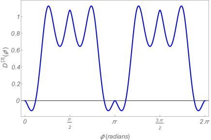
Figure 1: (Color online) Information deficit $\mathcal{D}^{[3]}(\phi)$ plotted against dimensionless parameter $\phi(=(\frac{\Delta_{21}L}{2\hbar cE})$ for two flavor approximation in vacuum and three measurements made at $t_{0},t_{1}$ and $t_{2}$ ($t_{0}<t_{1}<t_{2}$). The negative values of $D^{[3]}(\phi)$ correspond to the violation of ELGI. The values of the mixing angle $\theta_{12}$ and mass squared difference $\Delta_{21}$ are chosen to be $33.48^{o}$ and $7.5\times 10^{-5}eV^{2}$, respectively. The result is independent of the initial state chosen, since the survival and oscillation probabilities have same form irrespective of the initial state. The maximum negative value (measure of the strength of violation) acquired by $\mathcal{D}^{[3]}(\phi)$ is $-0.1193$.

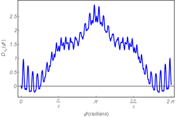
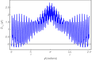
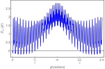
Figure 2: (Color online) Three flavor scenario in vacuum. Information deficit $\mathcal{D}_{\nu_{x}}^{[3]}(\phi)(x=e,\mu,\tau)$ plotted against dimensionless parameter $\phi(=(\frac{\Delta_{21}L}{2\hbar cE})$. The various neutrino parameters used are as: $\theta_{12}=33.48^{o},~{}\theta_{13}=8.50^{o},~{}\theta_{23}=42.3^{o},~{}\Delta_{21}=7.5\times 10^{-5}~{}eV^{2},~{}\Delta_{32}=~{}\Delta_{31}=2.457\times 10^{-3}~{}eV^{2}$. The top-left, top-right and bottom figures correspond to the cases with initial state $\nu_{e}$, $\nu_{\mu}$ and $\nu_{\tau}$, respectively. The maximum negative value of the information difference is a measure of the strength of the entropic violation and in this case, turn out to be $Min[\mathcal{D}_{e}^{[3]}(\phi)]\approx-0.2196$ at $\phi\approx 5.7527~{}radians$, $Min[\mathcal{D}_{\mu}^{[3]}(\phi)]\approx-0.2151$ at $\phi\approx 5.7527~{}radians$, $Min[\mathcal{D}_{\uptau}^{[3]}(\phi)]\approx-0.2189$ at $\phi\approx 5.7527~{}radians$.

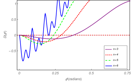
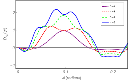
Figure 3: (Color online) Information difference $\mathcal{D}^{[n]}(\phi)$ plotted against dimensionless parameter $\phi$ for different values of $n$, the number of observations made on the system. The left and right panels correspond to the two and three flavor cases, in vacuum, respectively. It is clear that, as the number of measurements $n$ increases, the information difference becomes more and more negative. In other words, the maximum negative value of $\mathcal{D}^{[n]}(\phi)$ increases with the increase in the number of measurements. The subscript $\nu_{e}$ shows that the initial state for the three flavor case is chosen to be $\ket{\nu_{e}}$.

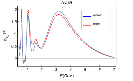
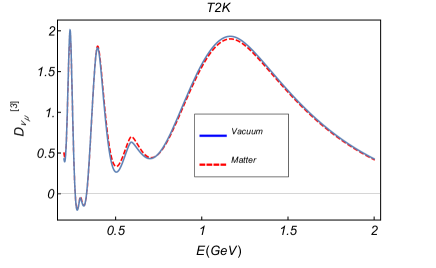
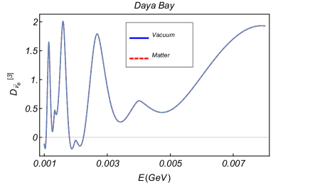
Figure 4: (Color online) Information deficit $\mathcal{D}^{[3]}$ as a function of neutrino energy in three flavor scenario of neutrino oscillation. The top-left, top-right bottom plots correspond to NO$\nu$A, T2K and Daya-Bay experiments, respectively. Solid and dashed curves show the variation of $\mathcal{D}^{[3]}$ in matter and vacuum, respectively. The baseline for NO$\nu$A experiments is 810 km and the energy of the neutrinos varies between 0.5 GeV to 10 GeV. For of T2K experiment, the neutrinos pass through a baseline of 295 km with the energy upto 2 GeV. While as in Daya-Bay experiment, neutrino energy is of the order of few MeVs. It is clear that the matter effect is prominent in long baseline and high energy experiments like NO$\nu$A than in the small baseline and low energy experiments (T2K and Daya-Bay). The initial flavor in both the accelerator experiments NO$\nu$A and T2K is $\nu_{\mu}$, while in the reactor Daya-Bay experiment, the initial state is the electron anti-neutrino $\bar{\nu}_{e}$.

IV Time evolution of $B$ and $K$ meson systems

In this section we spell out the time evolution of B(K) meson system in the lexicon of open quantum systems. The quantum system is in reality an open system interacting with its environment. This leads to decoherence, the process of loosing the quantum coherence. The study of such decoherence in elementary particles has been a topic of great interest Ellis et al. (1984); Huet and Peskin (1995); Ellis et al. (1996); Bertlmann et al. (1999, 2003); Banerjee et al. (2016); Alok et al. (2015).

We start by assuming that the Hilbert space is the direct sum $H_{B^{o}}\bigoplus H_{0}$, spanned by the orthonormal basis $\ket{B^{o}}=\begin{bmatrix}1&0&0\end{bmatrix}^{T}$, $\ket{\bar{B}^{o}}=\begin{bmatrix}0&1&0\end{bmatrix}^{T}$ and $\ket{0}=\begin{bmatrix}0&0&1\end{bmatrix}^{T}$, with $\langle B^{o}|B^{o}\rangle=\langle\bar{B}^{o}|\bar{B}^{o}\rangle=\langle 0|0\rangle=\mathbb{1}$ and $\langle B^{o}|\bar{B}^{o}\rangle=\langle B^{o}|0\rangle=\langle\bar{B}^{o}|0\rangle=0$. However, the flavor states are not the eigenstates of the time evolution but are related to the stationary states $\{B_{H},B_{L}\}$ by the following equations

$$\ket{B^{o}}=\frac{1}{2p}\bigg{(}\ket{B_{L}}+\ket{B_{H}}\bigg{)};\qquad\ket{\bar{B}^{o}}=\frac{1}{2q}\bigg{(}\ket{B_{L}}-\ket{B_{H}}\bigg{)}.$$ (22)

Due to normalization $|p|^{2}+|q|^{2}=1$ and $\langle B_{H}|B_{L}\rangle=|p|^{2}-|q|^{2}$. The existence of CP violation is implied by $|\frac{p}{q}|\neq 1$.

The evolution of the system is represented by the operator-sum representation Kraus (1983)

$$\rho(t)=\sum_{i=0}^{5}\mathcal{K}_{i}(t)\rho(0)\mathcal{K}^{\dagger}_{i}(t),$$ (23)

where $\mathcal{K}_{i}(t)$ are the Kraus operators with the following form:

$$\left.\begin{array}[]{r@{\;}l}\mathcal{K}_{0}=&\ket{0}\bra{0},\\ \\ \mathcal{K}_{1}=&\mathcal{C}_{1+}\big{(}\ket{B^{0}}\bra{B^{0}}+\ket{\bar{B}^{0}}\bra{\bar{B}^{0}o}\big{)}+\mathcal{C}_{1-}\big{(}\frac{p}{q}\ket{B^{0}}\bra{\bar{B}^{0}}+\frac{q}{p}\ket{\bar{B}^{0}}\bra{B^{0}}\big{)},\\ \\ \mathcal{K}_{2}=&\mathcal{C}_{2}\big{(}\frac{p+q}{2p}\ket{0}\bra{B^{0}}+\frac{p+q}{2q}\ket{0}\bra{\bar{B}^{0}}\big{)},\\ \\ \mathcal{K}_{3}=&\mathcal{C}_{3+}\frac{p+q}{2p}\ket{0}\bra{B^{0}}+\mathcal{C}_{3-}\frac{p+q}{2q}\ket{0}\bra{\bar{B}^{0}},\\ \\ \mathcal{K}_{4}=&\mathcal{C}_{4}\big{(}\ket{B^{0}}\bra{B^{0}}+\ket{\bar{B}^{0}}\bra{\bar{B}^{0}}+\frac{p}{q}\ket{B^{0}}\bra{\bar{B}^{o}}+\frac{q}{p}\ket{\bar{B}^{0}}\bra{B^{0}}\big{)},\\ \\ \mathcal{K}_{5}=&\mathcal{C}_{5}\big{(}\ket{B^{0}}\bra{B^{0}}+\ket{\bar{B}^{0}}\bra{\bar{B}^{0}}-\frac{p}{q}\ket{B^{0}}\bra{\bar{B}^{0}}-\frac{q}{p}\ket{\bar{B}^{0}}\bra{B^{0}}\big{)}.\end{array}\right\}$$ (24)

The coefficients are given by $\mathcal{C}_{1\pm}=\frac{1}{2}\left[e^{-(2im_{L}+\Gamma_{L}+\lambda)t/2}\pm e^{-(2im_{H}+\Gamma_{H}+\lambda)t/2}\right]$,
$\mathcal{C}_{2}=\sqrt{\frac{Re[\frac{p-q}{p+q}]}{|p|^{2}-|q|^{2}}\big{(}1-e^{-\Gamma_{L}t}-(|p|^{2}-|q|^{2})^{2}\frac{|1-e^{-(\Gamma+\lambda-i\Delta m)t}|^{2}}{1-e^{-\Gamma_{H}t}}}\big{)}$, $\mathcal{C}_{3\pm}=\sqrt{\frac{Re[\frac{p-q}{p+q}]}{(|p|^{2}-|q|^{2})(1-e^{-\Gamma_{H}t})}}\big{[}1-e^{-\Gamma_{H}t}\pm(1-e^{-(\Gamma+\lambda-i\Delta m)t})(|p|^{2}-|q|^{2})\big{]}$, $\mathcal{C}_{4}=\frac{e^{-\Gamma_{L}t/2}}{2}\sqrt{1-e^{-\lambda t}}$ and $\mathcal{C}_{5}=\frac{e^{-\Gamma_{H}t/2}}{2}\sqrt{1-e^{-\lambda t}}$. Here $p$ and $q$ are as defined in Eq. (22). $\Gamma_{L}$($\Gamma_{H}$) is the decay width of $B^{o}_{L}$($B^{o}_{H}$), $\Gamma=0.5(\Gamma_{L}+\Gamma_{H})$ is the average decay width. $m_{H}$$(m_{L})$ is the mass of $B_{H}$($B_{L}$) and $\Delta m=m_{H}-m_{L}$ is the mass difference. $\lambda$ is the decoherence parameter which quantifies the strength of the interaction between the one particle system and its environment.

If the meson starts at time $t=0$ in state $\ket{B^{o}}$ or $\ket{\bar{B}^{o}}$, then at some later time $t$, the state is given by Eqns. (25) and (26), respectively.

$$\rho_{B^{0}}(t) =\frac{1}{2}e^{-\Gamma t}\begin{pmatrix}\cosh(\frac{\Delta\Gamma}{2})+e^{-\lambda t}\cos(\Delta mt)~{}~{}~{}&(\frac{q}{p})^{*}(-\sinh(\frac{\Delta\Gamma}{2})-ie^{-\lambda t}\sin(\Delta mt)&0\\ \\ (\frac{q}{p})(-\sinh(\frac{\Delta\Gamma}{2})+ie^{-\lambda t}\sin(\Delta mt))~{}~{}~{}&|\frac{q}{p}|^{2}\cosh(\frac{\Delta\Gamma}{2})-e^{-\lambda t}\cos(\Delta mt)&0\\ \\ 0~{}~{}~{}&0&\rho_{33}(t)\end{pmatrix},$$ (25)

$$\rho_{\bar{B}^{0}}(t) =\frac{1}{2}e^{-\Gamma t}\begin{pmatrix}|\frac{p}{q}|^{2}(\cosh(\frac{\Delta\Gamma}{2})-e^{-\lambda t}\cos(\Delta mt))~{}~{}&(\frac{p}{q})(-\sinh(\frac{\Delta\Gamma}{2})+ie^{-\lambda t}\sin(\Delta mt))&0\\ \\ (\frac{p}{q})^{*}(-\sinh(\frac{\Delta\Gamma}{2})-ie^{-\lambda t}\sin(\Delta mt))&\cosh(\frac{\Delta\Gamma}{2})+e^{-\lambda t}\cos(\Delta mt)&0\\ \\ 0&0&\tilde{\rho}_{33}(t)\\ \end{pmatrix},$$ (26)

where $\Delta\Gamma=\Gamma_{H}-\Gamma_{L}$, $\rho_{33}(t)$ and $\tilde{\rho}_{33}(t)$ are complicated functions. The same description holds for the case of $K$ meson system with appropriate notational changes. The diagonal elements give survival and transition probabilities

$$P_{B^{o}\rightarrow B^{o}}(t) =\frac{1}{2}e^{-\Gamma t}\bigg{[}\cosh(\frac{\Delta\Gamma}{2})+e^{-\lambda t}\cos(\Delta mt)\bigg{]},$$ (27)

$$P_{B^{o}\rightarrow\bar{B}^{o}}(t) =\frac{1}{2}e^{-\Gamma t}\bigg{[}|\frac{q}{p}|^{2}\cosh(\frac{\Delta\Gamma}{2})-e^{-\lambda t}\cos(\Delta mt)\bigg{]}.$$ (28)

Similarly, we can define probabilities like $P_{\bar{B}^{o}\rightarrow B^{o}}(t)$, $P_{\bar{B}^{o}\rightarrow\bar{B}^{o}}(t)$, $P_{\bar{B}^{o}\rightarrow 0}(t)$.

Based on the above discussion, we show in Fig. (5) the probabilities for the case of K and B meson systems. The sub-figure, in case of $K$ system, highlights a region between $\Delta t=0~{}to~{}10\tau_{K}$. It can be seen that the K meson system retains coherence for much longer time, consistent with the findings reported in Banerjee et al. (2016).

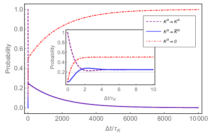
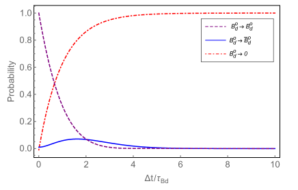
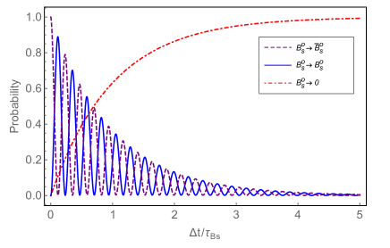
Figure 5: (Color online) Probabilities: The top-left, top-right and bottom figures depict the probabilities plotted w.r.t the dimensionless quantity $\Delta t/\uptau$ for the $K$, $B_{d}$ and $B_{s}$ mesons, respectively. Here $\Delta t$ is the time between successive measurements and $\tau$ is the mean life time of respective mesons. For the $K$ system, the mean life time is $\uptau_{K}=1.7889\times 10^{-10}s$. Also, $\Gamma=5.59\times 10^{9}~{}{\rm s^{-1}}$, $\Delta\Gamma=1.1174\times 10^{10}~{}{\rm s^{-1}}$, $\lambda=2.0\times 10^{8}~{}{\rm s^{-1}}$ and $\Delta m=5.302\times 10^{9}~{}{\rm s^{-1}}$ Patrignani et al. (2016). Here we used $Re(\epsilon)=1.596\times 10^{-3}$ and $|\epsilon|=2.228\times 10^{-3}$ D’Ambrosio et al. (2006). For the $B_{d}$ system, $\uptau_{B_{d}}=1.518\times 10^{-12}s$, $\Gamma=6.58\times 10^{11}~{}{\rm s^{-1}}$, $\Delta\Gamma=0$, $\lambda=0.012\times 10^{12}~{}{\rm s^{-1}}$ Alok et al. (2015) and $\Delta m=0.5064\times 10^{12}~{}{\rm s^{-1}}$ Amhis et al. (2017). The $CP$ violating parameter used here is $|\frac{q}{p}|=1.010$ Amhis et al. (2017). Finally, for the $B_{s}$ meson, $\uptau_{B_{s}}=1.509\times 10^{-12}s$, $\Gamma=0.6645\times 10^{12}~{}{\rm s^{-1}}$, $\Delta\Gamma=0.086\times 10^{12}~{}{\rm s^{-1}}$, $\lambda=0.012\times 10^{12}~{}{\rm s^{-1}}$ and $\Delta m=17.757\times 10^{12}~{}{\rm s^{-1}}$ Amhis et al. (2017). The value of the $CP$ violating parameter here is $|\frac{q}{p}|=1.003$ Amhis et al. (2017).

Entropic Leggett-Garg inequality for $B$ and $K$ meson systems:
In this case, the joint probability $P(a_{2},a_{1})$ is constructed in terms of the Kraus operators defined in Eq. (24) as

$$P(a_{2},a_{1})=Tr\Big{\{}\Pi^{a_{2}}\sum\limits_{i=0}^{5}\mathcal{K}_{i}(t_{2}-t_{1})\Pi^{a_{1}}\rho(t_{1})\mathcal{K}^{\dagger}_{i}(t_{2}-t_{1})\Big{\}},$$ (29)

with $\Pi^{a_{i}}=|M\rangle\langle M|_{t_{i}}$ is the projector corresponding to the measurement at time $t_{i}$. In particular, if the meson is produced in flavor state $\ket{B^{o}}$ at time $t_{0}$ and a measurement is made at a later time $t_{1}$, then the mean conditional entropy, in terms of various probabilities is given by

$$H[A(t_{1})|A(t_{0})=B^{o}] =-P_{B^{o}\rightarrow B^{o}}(\Delta t)\log_{2}P_{B^{o}\rightarrow B^{o}}(\Delta t)$$

$$-P_{B^{o}\rightarrow\bar{B}^{o}}(\Delta t)\log_{2}P_{B^{o}\rightarrow\bar{B}^{o}}(\Delta t)$$

$$-P_{B^{o}\rightarrow 0}(\Delta t)\log_{2}P_{B^{o}\rightarrow 0}(\Delta t).$$ (30)

Here we have used $\Delta t=t_{1}-t_{0}$. Similarly we can calculate $H[A(t_{2})|A(t_{1})]$ and $H[A(t_{2})|A(t_{0})]$ and construct the simplest ELGI by invoking the stationarity assumption discussed in Sec. (III), such that the $n$-measurement inequality reads

$$\mathcal{D}^{[n]}(\Delta t)=(n-1)H(\Delta t)-H((n-1)\Delta t)\geq 0.$$ (31)

Hence, a violation of ELGI would imply negative values of $\mathcal{D}^{[n]}(\Delta t)$. We now discuss the various results obtained by studying the ELGI for neutrino and meson systems.

V Results and discussion

Figure (1) shows the variation of the information deficit $\mathcal{D}^{[3]}(\phi)$ in two flavor approximation for $n=3$, the number of measurements made on the system. Since the survival and oscillation probabilities, in two flavor approximation of neutrino oscillation, are independent of the initial state, so is the information difference $\mathcal{D}^{[3]}(\phi)$. The maximum negative value of $\mathcal{D}^{[3]}(\phi)$ is $-0.1193$. Fig. (2) depicts the same for three flavor case with different initial states. A clear violation of the ELGI is seen in all the cases. We find that the maximum negative value of $\mathcal{D}^{[3]}(\phi)$(measure of the strength of entropic violation) is same upto second decimal place, Min$[\mathcal{D}^{[3]}(\phi)]\approx-0.21$ occuring at $\phi\approx 5.75~{}radians$. Thus, the strength of violation in three flavor case in approximately twice as that of the two flavor scenaio, i.e., Min$[\mathcal{D}^{[3]}(\phi)]~{}(3-flavor)\approx 1.75$ and Min$[\mathcal{D}^{[3]}(\phi)~{}(2-flavor)]$. The maximum negative value for $\mathcal{D}^{[3]}(\phi)$ increases as we increase $n$-the number of measerements, as shown in Fig. (3). A similar trend was observed in Devi et al. (2013) for a quantum spin-$s$ system.

So far we discussed an ideal scenario of neutrinos propagating in vacuum and also talked about the $n$ time measurements. From the experimental point of view, the neutrinos do interact with matter, although the interaction is quite feeble. Also the possibility of putting up multiple detectors and making arbitrary number of measurements is difficult, given the present experimental facilities. Therefore, it is interesting to study the ELGtI in the context of some ongoing experiments. We will now discuss the violation of ELGtI by taking inputs parameters (viz., energy of neutrino, baseline and matter density) from the experiments like NO$\nu$A, T2K and Daya-Bay.

For the case when neutrinos pass through a constant matter density, one can obtain analytic form of the time evolution operator both in the flavor and mass basis Ohlsson and Snellman (2000c, a, 2001). In flavor basis, the time evolution operator $\mathcal{U}_{f}$ takes a state $\psi(t_{1})$ at time $t_{1}$ to $\psi(t_{2})$ at some late time $t_{2}$ such that $\psi(t_{2})=\mathcal{U}_{f}(t_{2}-t_{1})\psi(t_{1})$. In the ultra-relativistic limit $t\approx L$, where $L$ is the distance traveled by the neutrino. Apart from $L$, the time evolution operator depends on the energy of the neutrino $E_{n}$, the $CP$ violating phase $\delta$, the matter density parameter $A=\pm\sqrt{2}G_{F}N_{e}$ ($G_{F}$ is the Fermi coupling constant, $N_{e}$ is the electron density of the medium), the mixing angles ($\theta_{13}$, $\theta_{23}$, $\theta_{13}$) and the mass square differences ($\Delta_{21}$, $\Delta_{31}$, $\Delta_{32}$). Fig. (4) shows the variation of the deficit parameter $\mathcal{D}^{[3]}$ with the energy of the neutrinos for accelerator experiments like NO$\nu$A and T2K and the reactor Daya-Bay experiment in vacuum (red dashed) and matter (solid blue). It can be seen that the matter effect is more prominent in the long baseline and high energy experiment NO$\nu$A than the relatively short baseline and low energy experiments like T2K and Daya-Bay.

Figure (5) depicts the survival and transition probabilities for the decohering neutral $K$, $B_{d}$ and $B_{s}$ meson systems. The mean-lifetime of the neutral $K$ meson system is much longer than its $B$ meson counterpart. The information deficit is plotted in Fig. (6) for $K$, $B_{d}$ and $B_{s}$ systems. It is clear that the ELGI for three time measurement is violated in all the three cases. The extent of violation increases with the increase in the number of measurements $n$. Also, the time for which $\mathcal{D}^{[3]}$ remains negative (before it touches the classical limit 0), also increases with the increase in number of measurements. Analogous features were seen in Devi et al. (2013) in the context of a spin-$s$ system. The violation sustains for a much longer time in $K$ meson system than in $B_{d}$ and $B_{s}$ systems, bringing out the point that the $K$ meson system sustains its quantum behavior for a much longer time as compared to $B$ meson system, consistent with earlier works. The oscillatory behavior of $\mathcal{D}^{[3]}$, in the $B_{s}$ system, is because of the fact that the mass difference $\Delta m$ for $B_{s}$ system is nearly 35 times the value for the $B_{d}$ system and plays the role of frequency, in the form of terms like $\cos\Delta mt(\sin\Delta mt)$, in the state matrix and hence in the probabilities.

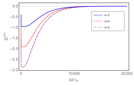
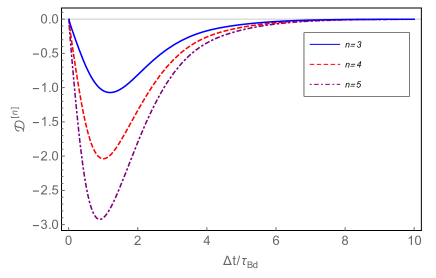
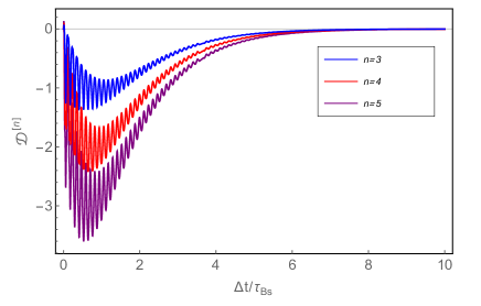
Figure 6: (Color online) Information deficit parameter $\mathcal{D}^{[n]}$ plotted against the dimensionless quantity $\Delta t/\uptau$, for different number of measurements $n$. The various parameters used are the same as used in Fig. (5).

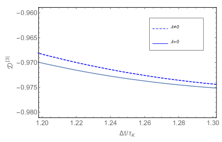
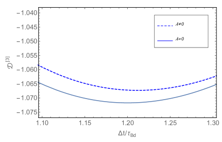
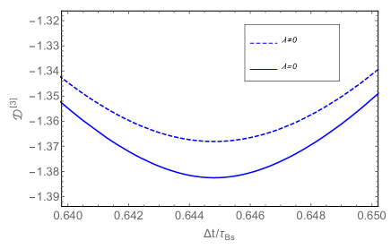
Figure 7: (Color online) Information deficit parameter $\mathcal{D}^{[3]}$ with and without decoherence. It can be seen that the non-zero value of the decoherence parameter $\lambda$ brings $\mathcal{D}^{[3]}$ closer to its classical limit, zero.

Decoherence is the process of loosing quantum coherence. In other words, the system comes close to the classical domain. It can be seen from Fig. (7) that the effect of decoherence is to bring the deficit parameter $\mathcal{D}^{[3]}$ closer to the classical value zero, as expected.

The ELGI for neutrino and meson systems given by Eqs. (21) and (31), respectively, are in terms of measurable quantities, i.e., the survival and transition probabilities. Several neutrino experiments like NO$\nu$A, T2K, Daya-Bay, use a neutrino source producing neutrinos in a particular state $\nu_{\mu}$ and the detector is sensitive to detect a particular flavor state $\nu_{e}$. Therefore, by using the experimentally observed probabilities at various energies, one can compute the information deficit parameter, thereby verifying the ELGI. For meson system, the state of a neutral meson is determined using the method of tagging. This allows one to determine the survival and transition probability of the neutral meson by identifying the charge of the lepton in its semileptonic decay. A knowledge of these probabilities would allow one to compute the deficit parameter and hence verify the ELGI.

VI Conclusion

In conclusion, we have studied the entropic Leggett-Garg inequality for neutrinos in the context of neutrino oscillation and for B and K meson systems by using the formalism of open quantum systems. For the neutrino system, ELGI violation in both two and three flavor neutrino scenarios is studied. The strength of entropic violation (quantified by the information deficit $\mathcal{D}^{[n]}$) in three flavor case is roughly twice that in two flavor case. In two flavor case, the probabilities are independent of the initial state, so is the deficit parameter. In the three flavor case, the probabilities are initial state dependent, while the maximum negative value of $\mathcal{D}^{[n]}$ (measure of the extent of violation), shows variation with initial state dependence, only beyond the second decimal place. The extent of violation (characterized by the negative value of $\mathcal{D}^{[n]}$ ) increases with the increase in $n$-the number of observations/measurements made on the system. In the limit of $n\rightarrow\infty$ and $\phi\rightarrow 0$, as shown in Fig. (8), the value of information deficit $\mathcal{D}^{[n]}(\phi)$ is always negative, implying that ELGI is always violated in this limit.

For the meson systems, decoherence and CP violating effects are taken into account. We found that the ELGI is violated in $K$, $B_{d}$ and $B_{s}$ systems, such that the violation persists for a much longer time in K meson system as compared to the $B_{d}$ and $B_{s}$ systems. Enhancement in the violation with the increase in the number of measurements is found and is consistent with earlier works. The effect of decoherence is found to take the deficit parameter closer to its classical value zero.

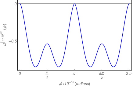
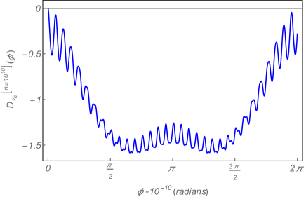
Figure 8: (Color online) Showing the the variation of the information dificit with the dimensionless parameter $\phi(=\frac{\Delta_{21}L}{2\hbar cE})$, for $n\approx 10^{10}$ in two (left) and three (right) flavor scenario of neutrino oscillations in vaccum. In three flavor case, the initial state is $\nu_{e}$. It is clear, that in the regime of large ’$n$’ and small ’$\phi$’, the value of the information deficit, $\mathcal{D}^{[n]}(\phi)$ is always negative.

References

- Heisenberg (1927) W. Heisenberg. Z. Phys. 43, 172 (1927).
- Bell (1964) J. S. Bell. Physics (Long Island City, N.Y.), 1, 195 (1964).
- Clauser et al. (1969) J. F. Clauser, M. A. Horne, A. Shimony, and R. A. Holt, Phys. Rev. Lett. 23, 880 (1969).
- Mermin (1993) N. D. Mermin, Rev. Mod. Phys. 65, 803 (1993).
- Aspect et al. (1982) A. Aspect, P. Grangier, and G. Roger, Phys. Rev. Lett. 49, 91 (1982).
- Tittel et al. (1998a) W. Tittel, J. Brendel, B. Gisin, T. Herzog, H. Zbinden, and N. Gisin, Phys. Rev. A, 57, 3229 (1998).
- Tittel et al. (1998b) W. Tittel, J. Brendel, H. Zbinden, and N. Gisin. Phys. Rev. Lett. 81, 3563, (1998).
- (8) G. Weihs, T. Jennewein, C. Simon, H. Weinfurter, and A. Zeilinger, Phys. Rev. Lett. 81, 5039 (1998).
- Pan et al. (2000) J. W. Pan, D. Bouwmeester, M. Daniell, H. Weinfurter, and A. Zeilinger, Nature, 403, 515 (2000).
- Rowe et al. (2001) M. A. Rowe et al., Nature, 409, 791 (2001).
- Salart et al. (2008) D. Salart, A. Baas, J. A. W. van Houwelingen, N. Gisin, and H. Zbinden, Phys. Rev. Lett. 100, 220404 (2008).
- (12) J. Kofler, S. Ramelow, M. Giustina, and A. Zeilinger, arXiv:1307.6475.
- Handsteiner et al. (2017) J. Handsteiner et al., Phys. Rev. Lett. 118, 060401 (2017).
- Rosenfeld et al. (2017) W. Rosenfeld et al., Phys. Rev. Lett. 119, 010402 (2017).
- Horodecki et al. (2009) R. Horodecki, P. Horodecki, M. Horodecki, and K. Horodecki. Rev. Mod Phys. 81, 865 (2009).
- (16) D. Cavalcanti and P. Skrzypczyk, arXiv:1604.00501.
- Brunner et al. (2014) N. Brunner, D. Cavalcanti, S. Pironio, V. Scarani, and S. Wehner. Rev. Mod. Phys. 86, 419 (2014).
- Ollivier and Zurek (2001) H. Ollivier and W. H. Zurek, Phys. Rev. Lett. 88, 017901 (2001).
- Henderson and Vedral (2001) L. Henderson and V. Vedral, J. Phys. A, 34, 6899 (2001).
- Adhikari and Banerjee (2012) S. Adhikari and S. Banerjee, Phys. Rev. A, 86, 062313 (2012).
- Aspect et al. (1981) A. Aspect, P. Grangier, and G. Roger, Phys. Rev. Lett. 47, 460 (1981).
- Tittel et al. (1998c) W. Tittel, J. Brendel, B. Gisin, T. Herzog, H. Zbinden, and N. Gisin, Phys. Rev. A 57, 3229 (1998).
- Tittel et al. (1998d) W. Tittel, J. Brendel, H. Zbinden, and N. Gisin, Phys. Rev. Lett. 81, 3563 (1998).
- Banerjee et al. (2010) S. Banerjee, V. Ravishankar, and R. Srikanth, Ann. Phys. 325, 816 (2010).
- Chakrabarty et al. (2011) I. Chakrabarty, S. Banerjee, and N. Siddharth, Quantum Information and Computation 11, 0541 (2011).
- Lanyon et al. (2013) B. Lanyon, P. Jurcevic, C. Hempel, M. Gessner, V. Vedral, R. Blatt, and C.F. Roos. Phys. Rev. Lett. 111, 100504 (2013).
- Kessel and Ermakov (2000) A. R. Kessel and V. L. Ermakov, arXiv quant-ph/0011002 (2000).
- Laflamme et al. (2001) R. Laflamme, D. G. Cory, C. Negrevergne, and L. Viola, arXiv quant-ph/0110029 (2001).
- Blasone et al. (2009) M. Blasone, F.abio Dell’Anno, S. De Siena, and F. Illuminati. Eur. Phys. Lett. 85, 50002 (2009).
- (30) A. K. Alok, S. Banerjee, and S Uma Sankar, Nucl. Phys. B, 909, 65 (2016).
- Banerjee et al. (2015) S. Banerjee, A. K. Alok, R. Srikanth, and B. C. Hiesmayr, Eur. Phys. J. C, 75, 487 (2015).
- Banerjee et al. (2016) S. Banerjee, A. K. Alok, and R. MacKenzie, Eur. Phys. J. Plus, 131, 129 (2016).
- (33) Khushboo Dixit, Javid Naikoo, Subhashish Banerjee, Ashutosh Kumar Alok, arXiv:1807.01546.
- Leggett and Garg (1985) A. J Leggett and A. Garg, Phys. Rev. Lett. 54, 857 (1985).
- Barbieri (2009) M. Barbieri. Phys. Rev. A 80, 034102 (2009).
- Avis et al. (2010) D. Avis, P. Hayden, and M. M. Wilde. Phys. Rev. A 82, 030102 (2010).
- Lambert et al. (2010) N. Lambert, C. Emary, Y. N. Chen, and F. Nori. Phys. Rev. Lett. 105, 176801 (2010).
- Lambert et al. (2011) N. Lambert, R. Johansson, and F. Nori. Phys. Rev. B 84, 245421 (2011).
- Montina (2012) A. Montina. Phys. Rev. Lett. 108, 160501 (2012).
- Emary et al. (2013) C. Emary, N. Lambert, and F. Nori. Rep. Prog. in Phys. 77, 016001 (2013).
- Kofler and Brukner (2013) J. Kofler and C. Brukner, Phys. Rev. A 87, 052115 (2013).
- (42) C. Emary. Phys. Rev. A 87, 032106 (2013).
- (43) J. Naikoo, A. K. Alok, S. Banerjee, S. Uma Sankar, G. Guarnieri, and B. C. Hiesmayr, arXiv:1710.05562.
- Fu and Chen (2017) Q. Fu and X. Chen, Eur. Phys. J. C, 77, 775 (2017).
- Naikoo et al. (2018) J. Naikoo, A. K. Alok, and S. Banerjee, Phys. Rev. D 97, 053008 (2018).
- Palacios-Laloy et al. (2010) A. Palacios-Laloy et al. Nat. Phys. 6, 442 (2010).
- Groen et al. (2013) J. Groen et al., Phys. Rev. Lett. 111, 090506 (2013).
- Goggin et al. (2011) M. Goggin et al., Proc. Nat. Acad. Sci., 108, 1256 (2011).
- Xu et al. (2011) J. S. Xu, C. F. Li, X. B. Zou, and G. C. Guo, Sci. Rep. 1, 101 (2011).
- Dressel et al. (2011) J. Dressel, C. Broadbent, J. Howell, and A. N. Jordan, Phys. Rev. Lett., 106, 040402 (2011).
- Suzuki et al. (2012) Y. Suzuki, M. Iinuma, and H. F. Hofmann, New J. Phys., 14, 103022 (2012).
- Athalye et al. (2011) V. Athalye, S. S. Roy, and T. S. Mahesh, Phys. Rev. Lett. 107, 130402 (2011).
- Souza et al. (2011) A. Souza, I. Oliveira, and R. Sarthour, New J. Phys. 13, 053023 (2011).
- Katiyar et al. (2013) H. Katiyar, A. Shukla, K. R. K. Rao, and T. S. Mahesh, Phys. Rev. A 87, 052102 (2013).
- Braunstein and Caves (1988) S. L. Braunstein and C. M. Caves, Phys. Rev. Lett. 61, 662 (1988).
- Chaves and Fritz (2012) R. Chaves and T. Fritz, Phys. Rev. A 85, 032113 (2012).
- Rastegin (2014) A. E. Rastegin, Communications in Theoretical Physics 62, 320 (2014).
- Morikoshi (2006) F. Morikoshi, Phys. Rev. A 73, 052308 (2006).
- Devi et al. (2013) A. R. Usha Devi, H. S. Karthik, A. K. Rajagopal, Phys. Rev. A 87, 052103 (2013).
- Kofler and Brukner (2008) J. Kofler and C. Brukner, Phys. Rev. Lett. 101, 090403 (2008).
- Fine (1982) A. Fine, Phys. Rev. Lett. 48, 291 (1982).
- Cover and Thomas (2012) T. M. Cover and J. A. Thomas, Elements of information theory (John Wiley & Sons), 2012.
- Bilenky et al. (1999) S. M. Bilenky, C. Giunti, and W. Grimus, Prog. Part. and Nucl. Phys. 43, 1 (1999).
- Gonzalez-Garcia and Maltoni (2008) M. C. Gonzalez-Garcia and M. Maltoni, Phys. Rep. 460, 1 (2008).
- Ohlsson and Snellman (2000a) T. Ohlsson and H. Snellman, J. Math. Phys. 41, 2768 (2000).
- Chau and Keung (1984) L. L. Chau and W. Y. Keung, Phys. Rev. Lett. 53, 1802 (1984).
- Giunti and Kim (2007) C. Giunti and C. W. Kim, Fundamentals of neutrino physics and astrophysics (Oxford university press, 2007).
- Barger et al. (1980) V. Barger, K. Whisnant, S. Pakvasa, and R. Phillips, Phys. Rev. D 22, 2718 (1980).
- Kim and Sze (1987) C. W. Kim and W. K. Sze, Phys. Rev. D 35, 1404 (1987).
- Zaglauer and Schwarzer (1988) H. Zaglauer and K. Schwarzer, Zeitschrift für Physik C Particles and Fields 40, 273 (1988).
- Ohlsson and Snellman (2000c) T. Ohlsson and H. Snellman, Phys. Lett. B 474, 153 (2000).
- Ohlsson and Snellman (2001) T. Ohlsson and H. Snellman,Eur. Phys. J. C 20, 507 (2001).
- Huelga et al. (1995) S. F. Huelga, T. W. Marshall, and E. Santos, Phys. Rev. A 52, R2497 (1995).
- Huelga et al. (1996) S. F. Huelga, T. W. Marshall, and E. Santos, Phys. Rev. A 54, 1798 (1996).
- Ellis et al. (1984) J. Ellis, J. S. Hagelin, D. V. Nanopoulos, and M. Srednicki, Nucl. Phys. B 241, 381 (1984).
- Huet and Peskin (1995) P. Huet and M. E. Peskin, Nucl. Phys. B 434, 3 (1995).
- Ellis et al. (1996) J. Ellis, J. L. Lopez, N. Mavromatos, and D. Nanopoulos, Phys. Rev. D 53, 3846 (1996).
- Bertlmann et al. (1999) R. A. Bertlmann, W. Grimus, B. C. Hiesmayr, Phys. Rev. D 60, 114032 (1999).
- Bertlmann et al. (2003) R. A. Bertlmann, K. Durstberger, and B. C. Hiesmayr, Phys. Rev. A 68, 012111 (2003).
- Alok et al. (2015) A. K. Alok, S. Banerjee, and S. Uma Sankar, Phys. Lett. B 749, 94 (2015).
- Kraus (1983) K. Kraus, States, effects and operations: fundamental notions of quantum theory (Springer, 1983).
- Patrignani et al. (2016) C. Patrignani et al., Chin. Phys C 40, 100001 (2016).
- D’Ambrosio et al. (2006) G. D’Ambrosio, G. Isidori, KLOE collaboration, et al., J. High Energy Phys. 2006, 011 (2006).
- Amhis et al. (2017) Y. Amhis et al., Eur. J. C. 77, 895 (2017).