Chirality Driven Helical Pattern Formation

Abstract

We study the pattern formation of chiral charges in the presence of reactions. We show that, in contrast to the original Turing’s mechanism of pattern formation in diffusion-reaction systems, the interplay between chiral effects and reactions can lead to a new kind of instability against spatially inhomogeneous perturbations, and furthermore, to a helical pattern formation, even without diffusion. This provides a new physical mechanism that can generate a macroscopic helical structure from microscopic chirality, including chirality of elementary particles, via nonequilibrium processes.

I Introduction

The notion of chirality is universally important in various areas of natural sciences ranging from physics and chemistry to biology. The helical motions and helical structures that possess right- or left-handed chirality appear over hierarchical scales from elementary particles (e.g., neutrinos), chemical molecules (e.g., amino acids) and biological polymers (e.g., DNA) to biological architectures (e.g., shells). It is generally considered that macroscopic helical structures are tied to microscopic chirality of the constituents. Although theoretical and experimental studies have been made on such connections for specific systems mostly in chemistry and biology, the generic physical mechanism to bridge between the different hierarchies has been elusive. In particular, the possible emergence of macroscopic helical structures from the most microscopic chirality to date—chirality of elementary particles—has been poorly understood.

In this paper, we provide a fundamentally new physical mechanism for the emergence of the macroscopic helical structure from microscopic chirality, including chirality of elementary particles, via nonequilibrium processes. We show that the chiral charges, in the presence of reactions and under certain conditions, lead to a new type of instability against spatially inhomogeneous perturbations, and furthermore, to a helical pattern formation, even without diffusion. Our mechanism should be contrasted with the Turing’s mechanism of pattern formation Turing ; Murray where diffusion plays an essential role. Our analysis is based on the effective theory and is independent of the details of systems. Hence, it is applicable to generic systems involving chiral charges, as long as the conditions that we shall derive are satisfied.

At a more technical level, the question that we address here can be seen from a different viewpoint. The conventional Turing instability and pattern formation Turing ; Murray is based on the diffusion equation that follows from the Fick’s law of diffusion, ${\bm{j}}=-D{\bm{\nabla}}n$ with $D$ the diffusion constant and $n$ the charge density, which necessarily generates entropy. However, it is known that, in some cases, there appear dissipationless currents originating from some topological nature of a system (see below). Then, one may ask a possible pattern formation due to such topological currents instead of diffusion currents. As we will see, our results provide an answer to such a question for the specific case where topological currents occur due to the chirality of elementary particles.

II Effective theory for chiral charges with reactions

To illustrate the essence of our mechanism for helical pattern formation, let us consider a 1+1 dimensional system. It is straightforward to extend our argument to other odd spatial dimensions (including 3+1 dimensions) where chirality is well defined.

Let us consider an effective theory for generic right- and left-handed charges, $n_{\rm R}(x,t)$ and $n_{\rm L}(x,t)$, in an open system with reactions. We define the vector and axial charges, $n_{\rm V}\equiv n_{\rm R}+n_{\rm L}$ and $n_{\rm A}\equiv n_{\rm R}-n_{\rm L}$, which transform under the parity transformation as $n_{\rm V}\rightarrow n_{\rm V}$ and $n_{\rm A}\rightarrow-n_{\rm A}$, respectively. In the presence of reactions, the generic effective theory for $n_{\rm V}$ and $n_{\rm A}$, which is consistent with parity symmetry, to leading order in derivatives is given by

$$\partial_{t}n_{\rm V} =\alpha_{1}\partial_{x}n_{\rm A}+\alpha_{2}n_{\rm A}\partial_{x}n_{\rm V}+\alpha_{3}n_{\rm V}\partial_{x}n_{\rm A}+f(n_{\rm V},n_{\rm A})+O(\partial_{x}^{2}),$$ (1a)

$$\partial_{t}n_{\rm A} =\beta_{1}\partial_{x}n_{\rm V}+\beta_{2}n_{\rm V}\partial_{x}n_{\rm V}+\beta_{3}n_{\rm A}\partial_{x}n_{\rm A}+g(n_{\rm V},n_{\rm A})+O(\partial_{x}^{2}).$$ (1b)

Here $\alpha_{1}$, $\alpha_{2}$, $\alpha_{3}$, $\beta_{1}$, $\beta_{2}$, and $\beta_{3}$ are some parity-invariant constants that depend on the microscopic details of the system, and $f(n_{\rm V},n_{\rm A})$ and $g(n_{\rm V},n_{\rm A})$ denote the reaction terms that are generically nonlinear functions of $n_{\rm V}$ and $n_{\rm A}$ and that make $n_{\rm V}$ and $n_{\rm A}$ nonconserved. From the requirement of parity symmetry, $f$ and $g$ satisfy the conditions, $f(n_{\rm V},-n_{\rm A})=f(n_{\rm V},n_{\rm A})$ and $g(n_{\rm V},-n_{\rm A})=-g(n_{\rm V},n_{\rm A})$. When some parity-breaking background field is present, additional terms, e.g., $\gamma_{1}\partial_{x}n_{\rm V}$ and $\gamma_{2}\partial_{x}n_{\rm A}$ with $\gamma_{1,2}$ being some parity-odd quantities, are added into the right-hand sides of Eqs. (1a) and (1b), respectively. The microscopic origin of the $\alpha$ and $\beta$ terms and the detailed forms of $f(n_{\rm V},n_{\rm A})$ and $g(n_{\rm V},n_{\rm A})$ as well as those of parity-breaking background fields will be irrelevant to the following discussion.

Note that, in a system involving only vector-type charges, which is the usual situation considered in the context of pattern formation Turing ; Murray , the $\alpha$ and $\beta$ terms in Eqs. (1) would be absent; the presence of these terms are specific to the system with chirality, and hence, they will be called the chiral terms. Note also that the diffusion terms of the form $D\partial_{x}^{2}n_{\rm V,A}$, which are typically leading order in derivatives (except for reaction terms), are included in $O(\partial^{2})$ and are higher order compared with the chiral terms.

Example of chiral terms

So far, our construction of the effective theory (1) has been general. Before proceeding further, we discuss one concrete realization of the chiral terms above by the topological transport phenomena in relativistic matter of chiral fermions: the so-called the chiral magnetic effect (CME) Vilenkin:1980fu ; Nielsen:1983rb ; Fukushima:2008xe and the chiral vortical effect (CVE) Vilenkin:1979ui ; Son:2009tf ; Landsteiner:2011cp , which are the currents along the direction of an external magnetic field ${\bm{B}}$ and a vorticity ${\bm{\omega}}$, respectively. The generic expressions of the vector and axial currents due to the CME and CVE at finite vector and axial chemical potentials, $\mu_{\rm V}$ and $\mu_{\rm A}$, and at finite temperature $T$ are given by

$${\bm{j}}_{\rm V} =\frac{\mu_{\rm A}}{2\pi^{2}}{\bm{B}+\frac{\mu_{\rm V}\mu_{\rm A}}{\pi^{2}}}{\bm{\omega}}\,,$$ (2)

$$\quad{\bm{j}}_{\rm A} =\frac{\mu_{\rm V}}{2\pi^{2}}{\bm{B}}+\left(\frac{\mu_{\rm V}^{2}+\mu_{\rm A}^{2}}{2\pi^{2}}+\frac{T^{2}}{6}\right){\bm{\omega}}\,,$$ (3)

respectively. Owing to the topological nature of chiral fermions, the transport coefficients (except for the $T$-dependent term) are exact independently of interactions Son:2012wh . Also, these currents are dissipationless and do not generate entropy Son:2009tf .

Inserting these expressions into the continuity equations for $n_{\rm V}$ and $n_{\rm A}$,

$$\partial_{t}n_{\rm V}+{\bm{\nabla}}\cdot{\bm{j}}_{\rm V}=0,\quad\partial_{t}n_{\rm A}+{\bm{\nabla}}\cdot{\bm{j}}_{\rm A}=0,$$ (4)

we obtain

$$\partial_{t}n_{\rm V} =-\frac{1}{2\pi^{2}\chi_{\rm A}}{\bm{B}}\cdot{\bm{\nabla}}n_{\rm A}-\frac{1}{\pi^{2}\chi_{\rm V}\chi_{\rm A}}(n_{\rm A}{\bm{\omega}}\cdot{\bm{\nabla}}n_{\rm V}+n_{\rm V}{\bm{\omega}}\cdot{\bm{\nabla}}n_{\rm A})\,,$$ (5a)

$$\partial_{t}n_{\rm A} =-\frac{1}{2\pi^{2}\chi_{\rm V}}{\bm{B}}\cdot{\bm{\nabla}}n_{\rm V}-\frac{1}{\pi^{2}\chi_{\rm V}^{2}}n_{\rm V}{\bm{\omega}}\cdot{\bm{\nabla}}n_{\rm V}-\frac{1}{\pi^{2}\chi_{\rm A}^{2}}n_{\rm A}{\bm{\omega}}\cdot{\bm{\nabla}}n_{\rm A}\,,\quad$$ (5b)

for a homogeneous temperature, where $\chi_{\rm V}$ and $\chi_{\rm A}$ are the susceptibilities defined by $\chi_{\rm V}\equiv{\partial\mu_{\rm V}}/{\partial n_{\rm V}}$ and $\chi_{\rm A}\equiv{\partial\mu_{\rm A}}/{\partial n_{\rm A}}$.

In particular, for the homogeneous magnetic field and global rotation that are aligned with each other, we can take ${\bm{B}}=B\hat{\bm{x}}$ and ${\bm{\omega}}=\omega\hat{\bm{x}}$ without loss of generality, and then the system is effectively reduced to 1+1 dimensions. In this case, we arrive at the terms that take exactly the same form as the chiral terms in Eqs. (1), where

$$\alpha_{1}=-\frac{B}{2\pi^{2}\chi_{\rm A}}\,,\quad\alpha_{2}=\alpha_{3}=-\frac{\omega}{\pi^{2}\chi_{\rm V}\chi_{\rm A}}\,,\quad$$ (6)

$$\beta_{1}=-\frac{B}{2\pi^{2}\chi_{\rm V}}\,,\quad\beta_{2}=-\frac{\omega}{\pi^{2}\chi_{\rm V}^{2}}\,,\quad\beta_{3}=-\frac{\omega}{\pi^{2}\chi_{\rm A}^{2}}\,.$$ (7)

In this example, the chiral terms in Eqs. (1) originate from the relativistic quantum effects related to the chirality of elementary particles. Note here that the diffusion term ${\bm{j}}=-D{\bm{\nabla}}n$ is higher order in derivatives compared with the CME and CVE if we take $B=O(\partial^{0})$ and $\omega=O(\partial^{0})$.

In the context of these chiral transport phenomena in both high-energy physics and condensed matter physics, however, effects of reactions have not been taken into account. Inclusion of reaction terms makes the right-hand sides of Eqs. (4) nonvanishing, which may exhibit new and rich physical phenomena. As we will see, the interplay between chiral effects and reactions in Eqs. (1) gives rise to a new type of instability and helical pattern formation. Note again that Eqs. (1), being an effective theory based on symmetries and systematic derivative expansion, are not limited to this particular realization due to the CME or CVE, and can be relevant to generic systems involving chiral charges.

III Linear stability analysis

We now study the linear stability of the system described by the effective theory (1). We assume that the system has a spatially homogeneous stable steady state $(n_{\rm V}$, $n_{\rm A})=(\bar{n}_{\rm V}$, $\bar{n}_{\rm A})$, and so $f(\bar{n}_{\rm V},\bar{n}_{\rm A})=g(\bar{n}_{\rm V},\bar{n}_{\rm A})=0$. We consider sufficiently small perturbations around this steady state,

$$n_{\rm V}=\bar{n}_{\rm V}+\delta n_{\rm V},\quad n_{\rm A}=\bar{n}_{\rm A}+\delta n_{\rm A},$$ (8)

so that the reaction terms can be expanded to linear order in $\delta n_{\rm V}$ and $\delta n_{\rm A}$ as

$$f(n_{\rm V},n_{\rm A})=f_{\rm V}\delta n_{\rm V}+f_{\rm A}\delta n_{\rm A},\quad g(n_{\rm V},n_{\rm A})=g_{\rm V}\delta n_{\rm V}+g_{\rm A}\delta n_{\rm A},$$ (9)

where $f_{\rm V}\equiv\left.{\partial f}/{\partial n_{\rm V}}\right|_{\rm ss}$, $f_{\rm A}\equiv\left.{\partial f}/{\partial n_{\rm A}}\right|_{\rm ss}$, $g_{\rm V}\equiv\left.{\partial g}/{\partial n_{\rm V}}\right|_{\rm ss}$, $g_{\rm A}\equiv\left.{\partial g}/{\partial n_{\rm A}}\right|_{\rm ss}$ are some constants that depend on the details of reactions (here “ss” stands for the steady state). From the consideration of parity symmetry, $f_{\rm V}$ and $g_{\rm A}$ are scalar while $f_{\rm A}$ and $g_{\rm V}$ are pseudoscalar. This is possible, e.g., if $f_{\rm A}\propto\bar{n}_{\rm A}$ and $g_{\rm V}\propto\bar{n}_{\rm A}$, and they can be nonzero when the steady state breaks parity symmetry by a nonzero $\bar{n}_{\rm A}$. Then, we have the linearized equations for Eqs. (1),

$$\partial_{t}\delta n_{\rm V} =\alpha_{\rm V}\partial_{x}\delta n_{\rm V}+\alpha_{\rm A}\partial_{x}\delta n_{\rm A}+f_{\rm V}\delta n_{\rm V}+f_{\rm A}\delta n_{\rm A},$$ (10a)

$$\partial_{t}\delta n_{\rm A} =\beta_{\rm V}\partial_{x}\delta n_{\rm V}+\beta_{\rm A}\partial_{x}\delta n_{\rm A}+g_{\rm V}\delta n_{\rm V}+g_{\rm A}\delta n_{\rm A},$$ (10b)

where $\alpha_{\rm V}\equiv\alpha_{2}\bar{n}_{\rm A}$, $\alpha_{\rm A}\equiv\alpha_{1}+\alpha_{3}\bar{n}_{\rm V}$, $\beta_{\rm V}\equiv\beta_{1}+\beta_{2}\bar{n}_{\rm V}$, $\beta_{\rm A}\equiv\beta_{3}\bar{n}_{\rm A}$. (In the presence of parity-breaking background fields, their contributions can be absorbed into $\alpha_{\rm V}$ and $\beta_{\rm A}$ accordingly.) We assume $\alpha_{\rm A}\beta_{\rm V}>0$, which ensures that the system is stable in the absence of reactions.

Let us take the temporally and spatially dependent (or spatially independent) perturbation of the form,

$$\delta n_{\rm V}=\epsilon_{\rm V}e^{\lambda t+iqx},\quad\delta n_{\rm A}=\epsilon_{\rm A}e^{\lambda t+iqx}.$$ (11)

We then get the matrix equation, $(M_{ij}+iqN_{ij}-\lambda I_{ij})x^{j}=0$, where

$$M\equiv\left(\begin{tabular}[]{cc}$f_{\rm V}$&$f_{\rm A}$\\ $g_{\rm V}$&$g_{\rm A}$\end{tabular}\right)\,,\quad N\equiv\left(\begin{tabular}[]{cc}$\alpha_{\rm V}$&$\alpha_{\rm A}$\\ $\beta_{\rm V}$&$\beta_{\rm A}$\end{tabular}\right)\,,\quad{\bm{x}}\equiv\left(\begin{tabular}[]{c}$\epsilon_{\rm V}$\\ $\epsilon_{\rm A}$\end{tabular}\right)\,,$$ (18)

and $I$ is the unit matrix. In order for it to have a nontrivial solution, we must have $\det(M+iqN-\lambda I)=0$, or

$$\lambda^{2}-[({\rm tr}M)+iq({\rm tr}N)]\lambda+(\det M-q^{2}\det N)+iq(\alpha_{\rm V}g_{\rm A}+\beta_{\rm A}f_{\rm V}-\alpha_{\rm A}g_{\rm V}-\beta_{\rm V}f_{\rm A})=0,$$ (19)

where ${\rm tr}M=f_{\rm V}+g_{\rm A}$, ${\rm tr}N=\alpha_{\rm V}+\beta_{\rm A}$, $\det M=f_{\rm V}g_{\rm A}-f_{\rm A}g_{\rm V}$, and $\det N=\alpha_{\rm V}\beta_{\rm A}-\alpha_{\rm A}\beta_{\rm V}$.

The stability conditions against the spatially homogeneous perturbations can be found from Eq. (19) with $q=0$ as

$${\rm tr}M<0,\quad\det M>0.$$ (20)

We now look for the condition that the steady state is unstable to a spatially inhomogeneous perturbation. This amounts to the condition that there must exist some real $q$, such that the real part of the solution to Eq. (19) is positive, ${\rm Re}\lambda>0$. This eventually reduces to the inequality,

$$\left[H(\alpha,\beta,f,g)-\alpha_{\rm A}\beta_{\rm V}({\rm tr}M)^{2}\right]q^{2}>({\rm tr}M)^{2}\det M,$$ (21)

where

$$H(\alpha,\beta,f,g)\equiv[\beta_{\rm V}f_{\rm A}+\alpha_{\rm A}g_{\rm V}+f_{\rm V}(\alpha_{\rm V}-\beta_{\rm A})][\beta_{\rm V}f_{\rm A}+\alpha_{\rm A}g_{\rm V}-g_{\rm A}(\alpha_{\rm V}-\beta_{\rm A})]\,.$$ (22)

Since the right-hand side of Eq. (21) is some positive constant from Eqs. (20), the necessary and sufficient condition for the existence of such $q$ is

$$H(\alpha,\beta,f,g)>\alpha_{\rm A}\beta_{\rm V}(f_{\rm V}+g_{\rm A})^{2}.$$ (23)

Apparently, in order for the condition (23) to be satisfied, nonzero chiral terms are necessary. Also, the steady state must explicitly break parity symmetry (otherwise $f_{\rm A}=g_{\rm V}=0$). Hence, we call this instability the “chirality-driven instability.”

It should be remarked that, in the original Turing mechanism Turing , diffusion drives the instability and pattern formation in open systems. On the other hand, in our case, the interplay between chiral effects and reactions leads to the instability (and furthermore, a helical pattern formation, as we shall see below) even without diffusion.

For $\alpha_{\rm V}=\beta_{\rm A}$ and $\alpha_{\rm A}=\beta_{\rm V}$, in particular, the condition (23) is simplified as

$$\alpha_{\rm A}\neq 0,\quad|f_{\rm A}+g_{\rm V}|>|f_{\rm V}+g_{\rm A}|\,.$$ (24)

In this case, it is convenient to move to the chiral basis in terms of $n_{\rm R}$ and $n_{\rm L}$, where the linearized equations of Eqs. (1) read

$$\partial_{t}\delta n_{\rm R} =\alpha_{\rm R}\partial_{x}\delta n_{\rm R}+F_{\rm R}\delta n_{\rm R}+F_{\rm L}\delta n_{\rm L},$$ (25a)

$$\partial_{t}\delta n_{\rm L} =\alpha_{\rm L}\partial_{x}\delta n_{\rm L}+G_{\rm R}\delta n_{\rm R}+G_{\rm L}\delta n_{\rm L},$$ (25b)

where $\alpha_{\rm R}\equiv\alpha_{\rm V}+\alpha_{\rm A}$, $\alpha_{\rm L}\equiv\alpha_{\rm V}-\alpha_{\rm A}$, $F_{\rm R}\equiv(f_{\rm V}+f_{\rm A}+g_{\rm V}+g_{\rm A})/2$, $F_{\rm L}\equiv(f_{\rm V}-f_{\rm A}+g_{\rm V}-g_{\rm A})/2$, $G_{\rm R}\equiv(f_{\rm V}+f_{\rm A}-g_{\rm V}-g_{\rm A})/2$, and $G_{\rm L}\equiv(f_{\rm V}-f_{\rm A}-g_{\rm V}+g_{\rm A})/2$. Then, the stability conditions against spatially homogenous perturbations in Eqs. (20) become

$$F_{\rm R}+G_{\rm L}<0,\quad F_{\rm R}G_{\rm L}-F_{\rm L}G_{\rm R}>0.$$ (26)

Also, the condition for the chirality-driven instability in Eq. (23) is rewritten as

$$\alpha_{\rm R}\neq\alpha_{\rm L},\quad F_{\rm R}G_{\rm L}<0\,,$$ (27)

which suggests that one of $F_{\rm R}$ or $G_{\rm L}$ is positive while the other is negative. The positive one may be called the activator, and the negative one the inhibitor. This has a somewhat similar structure to the Turing’s activator-inhibitor model Turing ; Murray , although the underlying mechanism leading to the instability is different.

IV Helical pattern formation

As a demonstration of the chirality-driven instability and helical pattern formation, we consider the following toy model for chiral charges, $n_{\rm R}(x,t)$ and $n_{\rm L}(x,t)$:

$$\partial_{t}n_{\rm R} =\alpha_{\rm R}\partial_{x}n_{\rm R}+F_{\rm R}n_{\rm R}+F_{\rm L}n_{\rm L}+\gamma n_{\rm R}^{3},$$ (28a)

$$\partial_{t}n_{\rm L} =\alpha_{\rm L}\partial_{x}n_{\rm L}+G_{\rm R}n_{\rm R}+G_{\rm L}n_{\rm L},$$ (28b)

where all the variables and coefficients are made dimensionless by certain rescaling (and, for simplicity of notation, we use the same variables and coefficients as before.) This model may be seen as describing fluctuation of chiral charges around the the parity-breaking background field (e.g., background axial charge $n_{\rm A}^{0}\neq 0$) for Eqs. (25). Here, the nonlinear $\gamma$ term is also added to stabilize the system.

Figure 1: Plots of $n_{\rm L}$ (left) and $n_{\rm R}$ (right) for the toy model (28) in the $(x,t)$ plane.

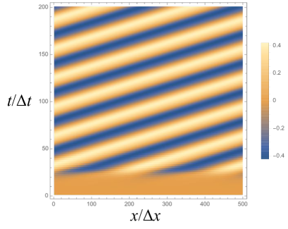
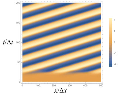
As an example, we take $\alpha_{\rm R}=0.5$, $\alpha_{\rm L}=0.1$, $F_{\rm R}=0.5$, $F_{\rm L}=-1.5$, $G_{\rm R}=1$, $G_{\rm L}=-2$, and $\gamma=-0.1$, such that the conditions (26) and (27) are satisfied. As an initial condition, we take a perturbation $n_{\rm R}(x,0)=\epsilon r_{\rm R}(x)$ and $n_{\rm L}(x,0)=\epsilon r_{\rm L}(x)$, where $r_{\rm R,L}(x)$ are uniform random functions in the interval $[-1,1]$ and $\epsilon=0.01$. In order to compute the time evolution of the initial perturbation, we perform the numerical simulation for 200 units of time with time step size $\Delta t=0.002$ and for 500 grid points with spatial grid size $\Delta x=0.002$. Then, we find $n_{\rm R,L}(x,t)$ at each spatial grid point $x=k\Delta x$ ($k=1,2,\cdots,500$) and at each time step $t=\ell\Delta t$ ($\ell=1,2,\cdots,200$).

The numerical result in the $(x,t)$ plane is shown in Fig. 1. This shows that the initial perturbation evolves into a propagating helical pattern in the $(x,t)$ plane—a feature that cannot be seen in the usual Turing pattern in 1+1 dimensions. This emergent macroscopic helical structure spontaneously breaks parity and both temporal and spatial translational symmetries (although the initial state does not). In particular, this result shows that microscopic chirality can generate a macroscopic helical structure via nonequilibrium processes even in the absence of diffusion.

This symmetry breaking pattern is reminiscent of the so-called “chiral soliton lattice” (CSL) that breaks parity and spatial translational symmetries. The CSL is realized as the ground state of various physical systems with chirality, such as cholesteric liquid crystals DeGennes , chiral magnets Dzyaloshinskii ; CM , and quantum chromodynamics at finite density in a magnetic field Brauner:2016pko and/or under a rotation Huang:2017pqe . Compared with the CSL in these systems, the parity- and translation-violating structure emerges via nonequilibrium processes in the present case. In passing, we also note that the resulting state here may be regarded as a nonequilibrium realization of the so-called time crystal Shapere:2012nq ; Richerme .

V Discussion and outlook

In this paper, we have demonstrated a new mechanism of chirality-driven instability and helical pattern formation due to the interplay between the chiral effects and reactions in open systems. Unlike the original Turing’s diffusion-driven instability, diffusion is irrelevant in our mechanism. Our mechanism, being based on the effective theory, is relevant to generic systems with chiral charges, as long as the conditions (20) and (23) are satisfied. In particular, it is applicable to chiral charges of elementary particles, where the emergence of macroscopic helical patterns is a consequence of topological currents (CME and/or CVE) associated with their chirality.

There are several future directions in which one can extend our analysis. (i) Effects of diffusion can be included as the higher-order correction to see how our mechanism is quantitatively modified. This study would clarify the competition or interplay between the chirality-driven instability and diffusion-driven instability. (ii) It is straightforward to generalize our effective theory (1) to 3+1 dimensions to study the helical pattern formation. One such direction is to solve Eqs. (5) for inhomogeneous magnetic fields and/or rotation in the presence of reactions. (iii) Since chirality is defined only in odd spatial dimensions, our mechanism of the chirality-driven instability is not directly applicable in two spatial dimensions. Still, one can ask if and how the topological currents in 2+1 dimensions, such as the quantum Hall effect, can lead to pattern formation without diffusion.

Finally but not least, it is an important question to understand whether and how our mechanism can be realized in actual physical systems. Concerning the chirality of elementary particles, it is typically considered that effects of parity violation by the weak interaction are too small to affect macroscopic helical structures Bonner2000 ; Avalos2000 . Even if so for each microscopic weak process, this is not necessarily the case in astrophysical systems. In fact, it has been recently argued that a core-collapse supernova is the system with the macroscopically largest parity violation in the Universe, where nonequilibrium electron capture reactions, ${\rm p}+{\rm e}_{\rm L}^{-}\rightarrow{\rm n}+\nu^{\rm e}_{\rm L}$, involving only left-handed electrons and neutrinos, produce large chirality asymmetries of leptons, and consequently, a strong helical magnetic field (which is equivalent to circularly polarized light), and helical fluid motion Yamamoto:2015gzz . Moreover, the length scale of magnetic fields and fluid motion there can be amplified to macroscopic scales by the inverse cascade of the chiral turbulence Masada:2018swb . Since the supernova is an open system with such large parity violation, our mechanism of the helical pattern formation may potentially be realized. This is just one possible example, and it would be interesting to investigate the relevance in other systems as well.

References

- (1) W. A. Bonner, Chirality 12, 114 (2000).
- (2) M. Avalos, R. Babiano, P. Cintas, J. L. Jimenez, and J. C. Palacios, Tetrahedron: Asymmetry 11, 2845 (2000).
- (3) A. M. Turing, Phils. Trans. R. Soc. London Ser. B, 273, 37 (1952).
- (4) J. D. Murray, Mathematical Biology II: Spatial Models and Biomedical Applications, 3rd ed. (Springer-Verlag, New York, 2003).
- (5) A. Vilenkin, Phys. Rev. D 22, 3080 (1980).
- (6) H. B. Nielsen and M. Ninomiya, Phys. Lett. B 130, 389 (1983).
- (7) K. Fukushima, D. E. Kharzeev, and H. J. Warringa, Phys. Rev. D 78, 074033 (2008).
- (8) A. Vilenkin, Phys. Rev. D 20, 1807 (1979).
- (9) D. T. Son and P. Surówka, Phys. Rev. Lett. 103, 191601 (2009).
- (10) K. Landsteiner, E. Megias, and F. Pena-Benitez, Phys. Rev. Lett. 107, 021601 (2011).
- (11) D. T. Son and N. Yamamoto, Phys. Rev. Lett. 109, 181602 (2012).
- (12) Y. Akamatsu and N. Yamamoto, Phys. Rev. Lett. 111, 052002 (2013).
- (13) P. G. de Gennes, Solid State Commun. 6, 163 (1968).
- (14) I. E. Dzyaloshinskii, Zh. Eksp. Teor. Fiz. 46, 1420 (1964) [Sov. Phys. JETP 19, 960 (1964)].
- (15) Y. Togawa, T. Koyama, K. Takayanagi, S. Mori, Y. Kousaka, J. Akimitsu, S. Nishihara, K. Inoue, A. S. Ovchinnikov, and J. Kishine, Phys. Rev. Lett. 108, 107202 (2012).
- (16) T. Brauner and N. Yamamoto, JHEP 1704, 132 (2017).
- (17) X. G. Huang, K. Nishimura, and N. Yamamoto, JHEP 1802, 069 (2018).
- (18) A. Shapere and F. Wilczek, Phys. Rev. Lett. 109, 160402 (2012); F. Wilczek, Phys. Rev. Lett. 109, 160401 (2012).
- (19) P. Richerme, Physics 10, 5 (2017).
- (20) N. Yamamoto, Phys. Rev. D 93, 065017 (2016).
- (21) Y. Masada, K. Kotake, T. Takiwaki, and N. Yamamoto, arXiv:1805.10419 [astro-ph.HE].