Synchronization of small oscillations

Abstract

Synchronization is studied in an array of identical oscillators undergoing small vibrations. The overall coupling is described by a pair of matrix-weighted Laplacian matrices; one representing the dissipative, the other the restorative connectors. A construction is proposed to combine these two real matrices in a single complex matrix. It is shown that whether the oscillators synchronize in the steady state or not depends on the number of eigenvalues of this complex matrix on the imaginary axis. Certain refinements of this condition for the special cases, where the restorative coupling is either weak or absent, are also presented.

1 Introduction

Consider the dynamics [8, Ch. 11]

$$M{\ddot{x}}+Kx=0$$ (1)

where $x\in{\mathbb{R}}^{n}$ and the matrices $M,\,K\in{\mathbb{R}}^{n\times n}$ are symmetric positive definite. This linear time-invariant differential equation, being the generalization of that of harmonic oscillator, plays an important role in mechanics. It emerges as the linearization of a Lagrangian system about a stable equilibrium and satisfactorily represents the behavior of the actual system undergoing small oscillations [1, Ch. 5]. Among examples obeying (1) are the $n$-link pendulum (Fig. 1) and the mass-spring system (Fig. 2). It is possible to find relevant systems outside the domain of mechanics as well. For instance, the LC circuit shown in Fig. 3 is also described by the form (1); see [15].

Figure 1: 3-link pendulum.

Figure 2: Mass-spring system.

Figure 3: LC oscillator.

Suppose now we take a number of identical $n$-link pendulums, each obeying (1), and couple them via passive components such as springs and dampers as shown in Fig. 4. Or, we gather a number of identical LC circuits and connect them through inductors and resistors as shown in Fig. 5. What can be said about the collective behavior of these arrays? In this paper we attempt to answer this question from the synchronization point of view. That is, we investigate conditions on the coupling that guarantee asymptotic synchronization throughout the array, where all the units tend to oscillate in unison despite the initial differences in their trajectories.

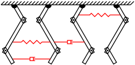
Figure 4: Coupled 3-link pendulums.

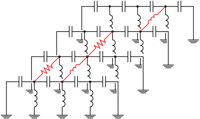
Figure 5: Coupled LC oscillators.

In studying synchronization stability the workhorse of the analysis is the matrix that describes the overall coupling, the ubiquitous Laplacian. The classical Laplacian matrix is a very useful representation of a graph with scalar-weighted edges. This matrix often appears in various network dynamics and its spectral properties have proved instrumental in understanding or establishing synchronization; see, for instance, [10, 9, 3, 4]. Although a single scalar-weighted Laplacian turns out to be quite able to represent the coupling in many different networks (which have been thoroughly investigated in the duly vast literature) significant exceptions do exist. One such exception we find appropriate to point out has to do with the case where the coupling can only be represented by a matrix-weighted Laplacian [15, 14, 17]. Another instance of deviation manifests itself in the array of harmonic oscillators linked simultaneously by both dissipative and restorative connectors [16], where two separate scalar-weighted Laplacians are required to account for the coupling in its entirety; one for the restorative, the other for the dissipative links. The particular problem we consider in this paper happens to fit to neither of these instances and instead contains them as special cases. Namely, the coupling of the array we study here cannot be properly described except by a pair of matrix-weighted Laplacians. To the best of our knowledge, the problem of synchronization of small oscillations has not yet been investigated under such direction and degree of generality. It is, of course, worthwhile to ask whether the suggested generalization is meaningful. In short, is it (in some sense) natural? We believe that it is; for two reasons. First, as we mentioned already, the dynamics we study can be realized by some very basic building blocks from physics and engineering: pendulum, spring, damper; or, capacitor, inductor, resistor. Second, some of the methods we develop in our analysis bear strong resemblance to classical tools from systems theory and graph theory, such as the Popov-Belevitch-Hautus (PBH) test for observability and the positivity check of the second smallest eigenvalue of the Laplacian for connectivity.

Somewhat imprecisely, we now give the statements of the three main results of this paper. Our setup, the array of $q$ oscillators, is described by three parameters (matrices): $P,\,L_{\rm d},\,L_{\rm r}$. (The precise problem statement and notation are given in Section 2.) The symmetric positive definite matrix $P\in{\mathbb{R}}^{n\times n}$ models the individual oscillator, where $n$ is the number of normal modes or characteristic frequencies. The matrix-weighted Laplacians $L_{\rm d},\,L_{\rm r}\in{\mathbb{R}}^{qn\times qn}$ represent, respectively, the dissipative coupling (e.g., dampers) and the restorative coupling (e.g., springs). Inspired by how the conductance ($g$) and susceptance ($b$) are brought together to form the admittance ($y=g+jb$) in circuit theory [2], we construct from our three matrices the single matrix $[L_{\rm d}+j([I_{q}\otimes P]+L_{\rm r})]$. In Section 3 we establish the following equivalence between this matrix and synchrony: The oscillators (asymptotically) synchronize if and only if $[L_{\rm d}+j([I_{q}\otimes P]+L_{\rm r})]$ has exactly $n$ eigenvalues on the imaginary axis. To develop a somewhat deeper understanding of this result we then dissect the matrix-weighted Laplacians $L_{\rm d},\,L_{\rm r}$ using the eigenvectors $v_{1},\,v_{2},\,\ldots,\,v_{n}$ of $P$ and obtain the collections of scalar-weighted Laplacians $G_{11},\,G_{22},\,\ldots,\,G_{nn}\in{\mathbb{R}}^{q\times q}$ and $B_{11},\,B_{22},\,\ldots,\,B_{nn}\in{\mathbb{R}}^{q\times q}$ through $G_{kk}=[I_{q}\otimes v_{k}^{T}]L_{\rm d}[I_{q}\otimes v_{k}]$ and $B_{kk}=[I_{q}\otimes v_{k}^{T}]L_{\rm r}[I_{q}\otimes v_{k}]$. These matrices are employed in Section 4 to show: For weak enough restorative coupling ($\|L_{\rm r}\|\ll 1$) the oscillators synchronize if every $[G_{kk}+jB_{kk}]$ has a single eigenvalue on the imaginary axis. Finally, in Section 5, we study the pure dissipative coupling scenario. There we find: In the absence of restorative coupling $(L_{\rm r}=0)$ the oscillators synchronize if and only if every $G_{kk}$ has a single eigenvalue at the origin.

2 Problem statement and notation

Consider the array of $q$ coupled oscillators (each of order $2n$) of the form

$$M{\ddot{x}}_{i}+Kx_{i}+\sum_{j=1}^{q}D_{ij}({\dot{x}}_{i}-{\dot{x}}_{j})+\sum_{j=1}^{q}R_{ij}(x_{i}-x_{j})=0\,,\qquad i=1,\,2,\,\ldots,\,q$$ (2)

where $x_{i}\in{\mathbb{R}}^{n}$ and $M,\,K,\,D_{ij},\,R_{ij}\in{\mathbb{R}}^{n\times n}$. Recall that $M=M^{T}>0$ and $K=K^{T}>0$. The matrices $D_{ij}^{T}=D_{ij}=D_{ji}\geq 0$ represent the dissipative coupling (due, e.g., to the dampers in the array of Fig. 4 or to the resistors in the array of Fig. 5) between the $i$th and $j$th oscillators. The matrices $R_{ij}^{T}=R_{ij}=R_{ji}\geq 0$ represent the restorative coupling (due, e.g., to the springs in the array of Fig. 4 or to the inductors in the array of Fig. 5) between the $i$th and $j$th oscillators. (We take $D_{ii}=0$ and $R_{ii}=0$.) Let $\sigma_{1},\,\sigma_{2},\,\ldots,\,\sigma_{n}$ be the roots of the polynomial $d(s)=\det(sM-K)$, i.e., the eigenvalues of $K$ with respect to $M$. Note that these $\sigma_{k}$ are also the eigenvalues of the matrix $P:=M^{-1/2}KM^{-1/2}$. Hence $\sigma_{k}>0$ for all $k$ because $P=P^{T}>0$. Our analysis will assume that these eigenvalues are distinct: $\sigma_{k}\neq\sigma_{\ell}$ for $k\neq\ell$. Under this assumption we here intend to arrive at conditions on the set of parameters $(M,\,K,\,(D_{ij})_{i,j=1}^{q},\,(R_{ij})_{i,j=1}^{q})$ under which the array (2) synchronizes, i.e., $\|x_{i}(t)-x_{j}(t)\|\to 0$ as $t\to\infty$ for all indices $i,\,j$ and all initial conditions $x_{1}(0),\,x_{2}(0),\,\ldots,\,x_{q}(0)$.

The identity matrix is denoted by $I_{q}\in{\mathbb{R}}^{q\times q}$. We let ${\mathbf{1}}_{q}\in{\mathbb{R}}^{q}$ denote the unit vector with identical positive entries, i.e., ${\mathbf{1}}_{q}=[1\ 1\ \cdots\ 1]^{T}/\sqrt{q}$. Given $X\in{\mathbb{C}}^{n\times n}$, we let $\lambda_{k}(X)$ denote the $k$th smallest eigenvalue of $X$ with respect to the real part. That is, ${\rm Re}\,\lambda_{1}(X)\leq{\rm Re}\,\lambda_{2}(X)\leq\cdots\leq{\rm Re}\,\lambda_{n}(X)$. The 2-norm of a vector $v\in{\mathbb{C}}^{n}$ is denoted by $\|v\|$. Recall that $\|v\|^{2}=v^{*}v$, where $v^{*}$ denotes the conjugate transpose of $v$. Likewise, $\|X\|$ denotes the induced 2-norm of the matrix $X$. Let $\mathcal{L}(q,\,n)\subset{\mathbb{R}}^{qn\times qn}$ denote the set of Laplacian matrices such that each $L\in\mathcal{L}(q,\,n)$ has the following structure

$$L=\left[\begin{array}[]{cccc}\sum_{j}W_{1j}&-W_{12}&\cdots&-W_{1q}\\ -W_{21}&\sum_{j}W_{2j}&\cdots&-W_{2q}\\ \vdots&\vdots&\ddots&\vdots\\ -W_{q1}&-W_{q2}&\cdots&\sum_{j}W_{qj}\end{array}\right]=:{\rm lap}\,(W_{ij})_{i,j=1}^{q}$$

where the weights $W_{ij}\in{\mathbb{R}}^{n\times n}$ satisfy $W_{ij}^{T}=W_{ij}=W_{ji}\geq 0$ with $W_{ii}=0$. Observe the symmetry $L=L^{T}$ and the positive semidefiniteness ${\mathbf{x}}^{*}L{\mathbf{x}}=\sum_{j>i}(x_{i}-x_{j})^{*}W_{ij}(x_{i}-x_{j})\geq 0$, where ${\mathbf{x}}=[x_{1}^{T}\ x_{2}^{T}\ \cdots\ x_{q}^{T}]^{T}\in({\mathbb{C}}^{n})^{q}$. Also ${\rm null}\,L\supset{\rm range}\,[{\mathbf{1}}_{q}\otimes I_{n}]$, where $\otimes$ is the Kronecker product symbol.

All the positive (semi)definite matrices we consider in this paper will be (real and) symmetric. Therefore henceforth we write $X>0$ ($X\geq 0$) to mean $X^{T}=X>0$ ($X^{T}=X\geq 0$). A simple fact from linear algebra that we frequently use in our analysis is

$$X\geq 0\ \ \mbox{and}\ \ \xi^{*}X\xi=0\implies X\xi=0$$

where $\xi$ is a vector of appropriate size. Another fact that will receive frequent visits is the following.

Fact 1

Let both $X,\,Y\in{\mathbb{R}}^{n\times n}$ be symmetric positive semidefinite. Then ${\rm Re}\,\lambda_{k}(X+jY)\geq 0$ for all $k$.

Proof. Let $\lambda\in{\mathbb{C}}$ be an eigenvalue of $X+jY$ and $\xi\in{\mathbb{C}}^{n}$ the corresponding unit eigenvector. We can write

$$\lambda=\xi^{*}(\lambda\xi)=\xi^{*}(X+jY)\xi=\xi^{*}X\xi+j\xi^{*}Y\xi$$ (4)

which yields ${\rm Re}\,\lambda=\xi^{*}X\xi\geq 0$ because $X,\,Y\geq 0$. The fact follows since $\lambda$ was arbitrary.   $\blacksquare$

3 Steady state solutions

Consider the array of coupled pendulums shown in Fig. 4 under arbitrary initial conditions. Devoid of any external interference, this assembly is unable to generate mechanical energy. Moreover, some of its initial energy will be gradually lost through the dampers as heat. The outcome is that in the long run the array has to settle into a constant energy state, the steady state. One way to show that the array synchronizes (if it does) therefore would be to establish that no steady state solution admits asynchronous oscillations. This is the approach we adopt for our analysis in this section.

Let us employ the coordinate change $z_{i}:=M^{1/2}x_{i}$ for $i=1,\,2,\,\ldots,\,q$. In the new coordinates, the array (2) takes the form

$${\ddot{z}}_{i}+Pz_{i}+\sum_{j=1}^{q}M^{-1/2}D_{ij}M^{-1/2}({\dot{z}}_{i}-{\dot{z}}_{j})+\sum_{j=1}^{q}M^{-1/2}R_{ij}M^{-1/2}(z_{i}-z_{j})=0\,,\qquad i=1,\,2,\,\ldots,\,q\,.$$ (5)

Recall that $P=M^{-1/2}KM^{-1/2}$ whose eigenvalues $\sigma_{1},\,\sigma_{2},\,\ldots,\,\sigma_{n}$ are distinct and positive. Let ${\mathbf{z}}=[z_{1}^{T}\ z_{2}^{T}\ \cdots\ z_{q}^{T}]^{T}$ and the matrices $L_{\rm d},\,L_{\rm r}\in\mathcal{L}(q,\,n)$ be constructed as

$$L_{\rm d} := {\rm lap}\,(M^{-1/2}D_{ij}M^{-1/2})_{i,j=1}^{q}\,,$$

$$L_{\rm r} := {\rm lap}\,(M^{-1/2}R_{ij}M^{-1/2})_{i,j=1}^{q}\,.$$

These Laplacian matrices allow us to express (5) as

$${\ddot{}{\mathbf{z}}}+[I_{q}\otimes P]{\mathbf{z}}+L_{\rm d}{\dot{}{\mathbf{z}}}+L_{\rm r}{\mathbf{z}}=0\,.$$ (6)

Note that the array (2) synchronizes (only) when the array (5) does. And the synchronization of the array (5) is equivalent to that every solution ${\mathbf{z}}(t)$ of (6) converges to the subspace ${\rm range}\,[{\mathbf{1}}_{q}\otimes I_{n}]$. Consider now the Lyapunov function

$$W({\mathbf{z}},\,\dot{}{\mathbf{z}})=\frac{1}{2}{\mathbf{z}}^{T}\left([I_{q}\otimes P]+L_{\rm r}\right){\mathbf{z}}+\frac{1}{2}{\dot{}{\mathbf{z}}}^{T}{\dot{}{\mathbf{z}}}$$

which is positive definite since $[I_{q}\otimes P]>0$ and $L_{\rm r}\geq 0$ imply $[I_{q}\otimes P]+L_{\rm r}>0$. The time derivative of this function along the solutions of (6) reads

$$\frac{d}{dt}W({\mathbf{z}}(t),\,\dot{}{\mathbf{z}}(t))=-\dot{}{\mathbf{z}}(t)^{T}L_{\rm d}\dot{}{\mathbf{z}}(t)\,.$$

Note that the righthand side is negative semidefinite since $L_{\rm d}\geq 0$. Hence by Lyapunov stability theorem each pair $({\mathbf{z}}(t),\,\dot{}{\mathbf{z}}(t))$ is bounded and by Krasovskii-LaSalle principle [7], every solution converges to some region contained in the set $\{({\mathbf{z}},\,\dot{}{\mathbf{z}}):\dot{W}({\mathbf{z}},\,\dot{}{\mathbf{z}})=0\}$. In other words, every steady state solution ${\mathbf{z}}_{\rm ss}(t)$ of (6) should identically satisfy $\dot{}{\mathbf{z}}_{\rm ss}(t)^{T}L_{\rm d}\dot{}{\mathbf{z}}_{\rm ss}(t)=0$, which (thanks to $L_{\rm d}\geq 0$) is equivalent to

$$L_{\rm d}\dot{}{\mathbf{z}}_{\rm ss}(t)\equiv 0\,.$$ (7)

Combining $\eqref{eqn:bigz}$ and (7) at once yields

$${\ddot{}{\mathbf{z}}}_{\rm ss}+([I_{q}\otimes P]+L_{\rm r}){\mathbf{z}}_{\rm ss}=0\,.$$ (8)

Let $p\leq qn$ be the number of distinct eigenvalues of $[I_{q}\otimes P]+L_{\rm r}$ and $\rho_{1},\,\rho_{2},\,\ldots,\,\rho_{p}>0$ denote these eigenvalues. Note that $\rho_{k}>0$ because $[I_{q}\otimes P]+L_{\rm r}>0$. Now, the solution to (8) has the form [1, §23]

$${\mathbf{z}}_{\rm ss}(t)={\rm Re}\sum_{k=1}^{p}e^{j\omega_{k}t}\xi_{k}$$ (9)

where $\omega_{k}=\sqrt{\rho_{k}}$ are distinct and positive, and each $\xi_{k}\in({\mathbb{C}}^{n})^{q}$ (some of which may be zero) satisfies

$$([I_{q}\otimes P]+L_{\rm r}-\omega_{k}^{2}I_{qn})\xi_{k}=0\,.$$ (10)

Note that the (7) and (9) imply

$$L_{\rm d}\xi_{k}=0$$ (11)

since $\omega_{k}$ are distinct and nonzero. Combining (10) and (11) we can write

$$\xi_{k}\in{\rm null}\left[\begin{array}[]{c}[I_{q}\otimes P]+L_{\rm r}-\omega_{k}^{2}I_{qn}\\ L_{\rm d}\end{array}\right]\,.$$ (14)

Suppose now the following (PBH test like) condition holds

$${\rm null}\left[\begin{array}[]{c}[I_{q}\otimes P]+L_{\rm r}-\lambda I_{qn}\\ L_{\rm d}\end{array}\right]\subset{\rm range}\,[{\mathbf{1}}_{q}\otimes I_{n}]\ \ \mbox{for all}\ \ \lambda\in{\mathbb{R}}\,.$$ (17)

Then (14) implies $\xi_{k}\in{\rm range}\,[{\bf 1}_{q}\otimes I_{n}]$ for all $k$. By (9) this readily yields ${\mathbf{z}}_{\rm ss}(t)\in{\rm range}\,[{\bf 1}_{q}\otimes I_{n}]$ for all $t$. Therefore (17) is sufficient for the array (2) to synchronize.

Let us also investigate the necessity. We begin by supposing that the condition (17) fails to hold. Then we can find an eigenvalue $\rho_{k}=\omega_{k}^{2}$ and an eigenvector $\xi\in({\mathbb{R}}^{n})^{q}$ satisfying $\xi\notin{\rm range}\,[{\mathbf{1}}_{q}\otimes I_{n}]$, $L_{\rm d}\xi=0$, and $([I_{q}\otimes P]+L_{\rm r}-\omega_{k}^{2}I_{qn})\xi=0$. Using the pair $(\omega_{k},\,\xi)$ let us construct the function $\zeta:{\mathbb{R}}\to({\mathbb{R}}^{n})^{q}$ as $\zeta(t)={\rm Re}\,(e^{j\omega_{k}t}\xi)$. This function satisfies the following properties. First, since $\xi\notin{\rm range}\,[{\mathbf{1}}_{q}\otimes I_{n}]$, we have

$$\zeta(t)=\xi\notin{\rm range}\,[{\bf 1}_{q}\otimes I_{n}]\ \ \mbox{for}\ \ t=0,\,T,\,2T,\,\ldots$$ (18)

where $T=2\pi/\omega_{k}$. Second, since $L_{\rm d}\xi=0$, we have at all times

$$L_{\rm d}\dot{\zeta}(t)={\rm Re}\,(j\omega_{k}e^{j\omega_{k}t}L_{\rm d}\xi)=0\,.$$ (19)

Third, since $([I_{q}\otimes P]+L_{\rm r}-\omega_{k}^{2}I_{qn})\xi=0$, we can write at all times

$${\ddot{\zeta}}(t)+([I_{q}\otimes P]+L_{\rm r})\zeta(t) = -\omega_{k}^{2}\zeta(t)+([I_{q}\otimes P]+L_{\rm r})\zeta(t)$$

$$= ([I_{q}\otimes P]+L_{\rm r}-\omega_{k}^{2}I_{qn}){\rm Re}\,(e^{j\omega_{k}t}\xi)$$

$$= {\rm Re}\,(e^{j\omega_{k}t}([I_{q}\otimes P]+L_{\rm r}-\omega_{k}^{2}I_{qn})\xi)$$

$$= 0$$

which together with (19) leads to

$${\ddot{\zeta}}(t)+[I_{q}\otimes P]\zeta(t)+L_{\rm d}\dot{\zeta}(t)+L_{\rm r}\zeta(t)\equiv 0\,.$$

Hence $\zeta(t)$ is a valid solution of (6). But it is clear from (18) that $\zeta(t)$ does not converge to ${\rm range}\,[{\bf 1}_{q}\otimes I_{n}]$. This means that the condition (17) is not only sufficient but also necessary for the synchronization of the array (2). We have therefore established:

Lemma 1

The array (2) synchronizes if and only if (17) holds.

We now convert the condition (17) to another form, which will prove more suitable for later analysis. To this end, we construct the complex matrix

$$\Gamma:=L_{\rm d}+j([I_{q}\otimes P]+L_{\rm r})\,.$$

A few observations on the spectrum of $\Gamma$ are in order. Note that $L_{\rm d}[{\mathbf{1}}_{q}\otimes v]=0$ for all $v\in{\mathbb{C}}^{n}$ thanks to $L_{\rm d}\in\mathcal{L}(q,\,n)$. The same goes for $L_{\rm r}$. Letting $v_{1},\,v_{2},\,\ldots,\,v_{n}\in{\mathbb{R}}^{n}$ be the (linearly independent) unit eigenvectors of $P$ corresponding to the eigenvalues $\sigma_{1},\,\sigma_{2},\,\ldots,\,\sigma_{n}$, respectively, we can thus write for $k=1,\,2,\,\ldots,\,n$

$$\Gamma[{\mathbf{1}}_{q}\otimes v_{k}] = L_{\rm d}[{\mathbf{1}}_{q}\otimes v_{k}]+j([I_{q}\otimes P][{\mathbf{1}}_{q}\otimes v_{k}]+L_{\rm r}[{\mathbf{1}}_{q}\otimes v_{k}])$$

$$= j[I_{q}\otimes P][{\mathbf{1}}_{q}\otimes v_{k}]$$

$$= j[(I_{q}{\mathbf{1}}_{q})\otimes(Pv_{k})]$$

$$= j\sigma_{k}[{\mathbf{1}}_{q}\otimes v_{k}]\,.$$

Therefore each $j\sigma_{k}$ is an eigenvalue of $\Gamma$ with the corresponding eigenvector $[{\mathbf{1}}_{q}\otimes v_{k}]$. Since $\sigma_{k}\neq\sigma_{\ell}$ for $k\neq\ell$ and the open left half plane contains no eigenvalue of $\Gamma$ by Fact 1; we can list, without loss of generality, the first $n$ eigenvalues as $\lambda_{k}(\Gamma)=j\sigma_{k}$ for $k=1,\,2,\,\ldots,\,n$. It turns out that the next eigenvalue in line is closely related to synchronization:

Lemma 2

The condition (17) holds if and only if ${\rm Re}\,\lambda_{n+1}(\Gamma)>0$.

Proof. Suppose ${\rm Re}\,\lambda_{n+1}(\Gamma)\leq 0$. This implies ${\rm Re}\,\lambda_{n+1}(\Gamma)=0$ because $\Gamma$ can have no eigenvalue with negative real part. Let therefore $\lambda_{n+1}(\Gamma)=j\beta$ with $\beta\in{\mathbb{R}}$. There are two possibilities. Either (i) $j\beta=j\sigma_{k}$ for some $k$ or (ii) not. Consider the case (i). Without loss of generality let us take $j\beta=j\sigma_{1}$. That is, the eigenvalue $j\sigma_{1}$ is repeated. Then there should be at least two linearly independent eigenvectors of $\Gamma$ corresponding to the eigenvalue $j\sigma_{1}$. To see this suppose otherwise. Then $[{\mathbf{1}}_{q}\otimes v_{1}]$ would be the only (unit) eigenvector associated to the eigenvalue $j\sigma_{1}$ and there would have to exist a generalized eigenvector $\xi_{1}\in({\mathbb{C}}^{n})^{q}$ satisfying $(\Gamma-j\sigma_{1}I_{qn})\xi_{1}=[{\mathbf{1}}_{q}\otimes v_{1}]$. This however would lead to the following contradiction

$$1=[{\mathbf{1}}_{q}\otimes v_{1}]^{T}[{\mathbf{1}}_{q}\otimes v_{1}]=[{\mathbf{1}}_{q}\otimes v_{1}]^{T}(\Gamma-j\sigma_{1}I_{qn})\xi_{1}=((\Gamma-j\sigma_{1}I_{qn})[{\mathbf{1}}_{q}\otimes v_{1}])^{T}\xi_{1}=0$$

since $\Gamma^{T}=\Gamma$. Therefore we can find an eigenvector $\xi\in({\mathbb{C}}^{n})^{q}$ corresponding to the eigenvalue $j\sigma_{1}$ satisfying $\xi\notin{\rm span}\,\{[{\mathbf{1}}_{q}\otimes v_{1}]\}$. Then it follows that

$$\xi\notin{\rm span}\,\{[{\mathbf{1}}_{q}\otimes v_{1}],\,[{\mathbf{1}}_{q}\otimes v_{2}],\,\ldots,\,[{\mathbf{1}}_{q}\otimes v_{n}]\}={\rm range}\,[{\mathbf{1}}_{q}\otimes I_{n}]\,.$$ (20)

As for the case (ii), i.e., $j\beta\neq j\sigma_{k}$ for all $k$, it is clear that an eigenvector of $j\beta$, call it $\xi$, should again satisfy (20). To sum up, whenever ${\rm Re}\,\lambda_{n+1}(\Gamma)\leq 0$, there exists a nonzero vector $\xi\in({\mathbb{C}}^{n})^{q}$ and a real number $\beta$ satisfying $\Gamma\xi=j\beta\xi$ and (20). Without loss of generality let $\|\xi\|=1$. Then (4) allows us to write

$$j\beta=\xi^{*}L_{\rm d}\xi+j\xi^{*}([I_{q}\otimes P]+L_{\rm r})\xi$$

which implies $L_{\rm d}\xi=0$. Then we can write $j\beta\xi=\Gamma\xi=j([I_{q}\otimes P]+L_{\rm r})\xi$, yielding $([I_{q}\otimes P]+L_{\rm r}-\beta I_{qn})\xi=0$. Hence $\xi$ satisfies

$$\xi\in{\rm null}\left[\begin{array}[]{c}[I_{q}\otimes P]+L_{\rm r}-\beta I_{qn}\\ L_{\rm d}\end{array}\right]\,.$$ (23)

Finally, combining (20) and (23) yields that the condition (17) cannot be true.

Now we show the other direction. Suppose (17) is not true. Then we can find $\beta\in{\mathbb{R}}$ and a vector $\xi\notin{\rm range}\,[{\mathbf{1}}_{q}\otimes I_{n}]$ that satisfy $L_{\rm d}\xi=0$ and $([I_{q}\otimes P]+L_{\rm r})\xi=\beta\xi$. This yields $\Gamma\xi=j\beta\xi$. By (20) we see that $\xi$ lies outside the subspace spanned by the linearly independent eigenvectors $[{\mathbf{1}}_{q}\otimes v_{1}],\,[{\mathbf{1}}_{q}\otimes v_{2}],\,\ldots,\,[{\mathbf{1}}_{q}\otimes v_{n}]$ of $\Gamma$. Recall that the eigenvalues associated to these eigenvectors are $j\sigma_{1},\,j\sigma_{2},\,\ldots,\,j\sigma_{n}$. Hence, together with $\xi$, there are at least $n+1$ linearly independent eigenvectors whose eigenvalues lie on the imaginary axis. This implies ${\rm Re}\,\lambda_{n+1}(\Gamma)$ cannot be strictly positive.   $\blacksquare$

Lemma 1 and Lemma 2 yield:

Theorem 1

The array (2) synchronizes if and only if ${\rm Re}\,\lambda_{n+1}(\Gamma)>0$.

To develop some insight on Theorem 1 we bring up some of its consequences concerning a number of special yet important cases. We first regenerate some known results on harmonic oscillators; then (in the following sections) we proceed to novel implications. Synchronization of coupled harmonic oscillators (i.e., the array (2) under $n=1$) is a thoroughly investigated problem; see, for instance, [11, 12, 18, 13]. Many interesting results have appeared recently, each of which studies a certain generalization of the nominal setup: an array of identical oscillators (e.g., 1-link pendulums) coupled only by dissipative components (e.g., dampers). In this simplest case synchronization is easy to understand. It is intuitively clear that if a pair of pendulums are connected by a damper then their motions have to have synchronized in the steady state. Consequently, the entire array synchronizes if its interconnection graph (where each node represents an oscillator and each edge a damper) is connected. This well-known, fundamental result makes the first corollary of Theorem 1 since the algebraic condition for a graph to be connected is that its Laplacian has a simple eigenvalue at the origin, i.e., its second smallest eigenvalue (also known as Fiedler eigenvalue) is positive.

Corollary 1

Suppose $n=1$ and $R_{ij}=0$ for all $i,\,j$. Then the array (2) synchronizes if and only if $\lambda_{2}(L_{\rm d})>0$.

Proof. That $n=1$ renders the matrix $P$ a real scalar. In particular, $P=\sigma_{1}$. We can therefore write

$${\rm Re}\,\lambda_{n+1}(\Gamma) = {\rm Re}\,\lambda_{n+1}(L_{\rm d}+j([I_{q}\otimes P]+L_{\rm r}))$$ (24)

$$= {\rm Re}\,\lambda_{2}(L_{\rm d}+j\sigma_{1}I_{q}+jL_{\rm r})$$

$$= {\rm Re}\,(\lambda_{2}(L_{\rm d}+jL_{\rm r})+j\sigma_{1})$$

$$= {\rm Re}\,\lambda_{2}(L_{\rm d}+jL_{\rm r})\,.$$

Now, $R_{ij}=0$ yields $L_{\rm r}=0$. Also, $L_{\rm d}\geq 0$ implies that all the eigenvalues of the Laplacian $L_{\rm d}$ are real. Hence

$${\rm Re}\,\lambda_{2}(L_{\rm d}+jL_{\rm r})=\lambda_{2}(L_{\rm d})\,.$$ (25)

The result follows by (24), (25), and Theorem 1.   $\blacksquare$

Corollary 1 has the following generalization covering the case where the 1-link pendulums are coupled by not only dampers, but also springs [16].

Corollary 2

Suppose $n=1$. Then the array (2) synchronizes if and only if ${\rm Re}\,\lambda_{2}(L_{\rm d}+jL_{\rm r})>0$.

Proof. Combine (24) and Theorem 1.   $\blacksquare$

4 Weak restorative coupling

In this section we study the synchronization of small oscillations under weak restorative coupling. To investigate how the strength of restorative coupling effects synchronization let us replace $R_{ij}$ in (2) with $\varepsilon R_{ij}$, yielding the dynamics

$$M{\ddot{x}}_{i}+Kx_{i}+\sum_{j=1}^{q}D_{ij}({\dot{x}}_{i}-{\dot{x}}_{j})+\varepsilon\sum_{j=1}^{q}R_{ij}(x_{i}-x_{j})=0\,,\qquad i=1,\,2,\,\ldots,\,q$$ (26)

where the scalar $\varepsilon>0$ represents the coupling strength. Our assumptions on the matrices $M,\,K,\,D_{ij},\,R_{ij}$ are same as before. A slight addition, however, is that we assume throughout this section that not all $R_{ij}$ are zero, i.e., $R_{ij}\neq 0$ for at least one pair $(i,\,j)$. The case where there is no restorative coupling (i.e., all $R_{ij}=0$) is studied in the next section. For our new array (26) let us define

$$\Gamma_{\varepsilon}:=L_{\rm d}+j([I_{q}\otimes P]+\varepsilon L_{\rm r})\,.$$

We infer from Theorem 1 that the array (26) synchronizes if and only if ${\rm Re}\,\lambda_{n+1}(\Gamma_{\varepsilon})>0$. Recall that $v_{1},\,v_{2},\,\ldots,\,v_{n}\in{\mathbb{R}}^{n}$ denote the (linearly independent) unit eigenvectors of $P$ corresponding to the distinct eigenvalues $\sigma_{1},\,\sigma_{2},\,\ldots,\,\sigma_{n}$, respectively. Since $P$ is real and symmetric the matrix $V=[v_{1}\ v_{2}\ \cdots\ v_{n}]$ is orthogonal, i.e., $V^{T}V=I_{n}$. Let $\Lambda={\mbox{\rm diag}}(\sigma_{1},\,\sigma_{2},\,\ldots,\,\sigma_{n})$. Note that $\Lambda=V^{T}PV$. Let us now construct the matrices $G,\,B\in{\mathbb{R}}^{qn\times qn}$ as

$$G=\left[\begin{array}[]{cccc}G_{11}&G_{12}&\cdots&G_{1n}\\ G_{21}&G_{22}&\cdots&G_{2n}\\ \vdots&\vdots&\ddots&\vdots\\ G_{n1}&G_{n2}&\cdots&G_{nn}\end{array}\right]\ ,\qquad B=\left[\begin{array}[]{cccc}B_{11}&B_{12}&\cdots&B_{1n}\\ B_{21}&B_{22}&\cdots&B_{2n}\\ \vdots&\vdots&\ddots&\vdots\\ B_{n1}&B_{n2}&\cdots&B_{nn}\end{array}\right]$$

where $G_{k\ell}=[I_{q}\otimes v_{k}^{T}]L_{\rm d}[I_{q}\otimes v_{\ell}]\in{\mathbb{R}}^{q\times q}$ and $B_{k\ell}=[I_{q}\otimes v_{k}^{T}]L_{\rm r}[I_{q}\otimes v_{\ell}]\in{\mathbb{R}}^{q\times q}$ for $k,\,\ell=1,\,2,\,\ldots,\,n$.

Lemma 3

The matrices $G_{kk},\,B_{kk}$ are Laplacian, i.e., $G_{kk},\,B_{kk}\in\mathcal{L}(q,\,1)$ for all $k=1,\,2,\,\ldots,\,n$.

Proof. We can write

$$G_{kk} = [I_{q}\otimes v_{k}^{T}]L_{\rm d}[I_{q}\otimes v_{k}]$$ (28)

$$= [I_{q}\otimes v_{k}^{T}]({\rm lap}\,(M^{-1/2}D_{ij}M^{-1/2})_{i,j=1}^{q})[I_{q}\otimes v_{k}]$$

$$= {\rm lap}\,(v_{k}^{T}M^{-1/2}D_{ij}M^{-1/2}v_{k})_{i,j=1}^{q}\,.$$

Likewise, $B_{kk}={\rm lap}\,(v_{k}^{T}M^{-1/2}R_{ij}M^{-1/2}v_{k})_{i,j=1}^{q}$.   $\blacksquare$

It is not difficult to see that the matrices $G,\,B$ satisfy

$$G&=\Pi^{T}[I_{q}\otimes V^{T}]L_{\rm d}[I_{q}\otimes V]\Pi\\ B=\Pi^{T}[I_{q}\otimes V^{T}]L_{\rm r}[I_{q}\otimes V]\Pi$$ (29)

where $\Pi\in{\mathbb{R}}^{qn\times qn}$ is the permutation matrix that yields $\Pi^{T}[X\otimes Y]\Pi=Y\otimes X$ for all $X\in{\mathbb{R}}^{q\times q}$ and $Y\in{\mathbb{R}}^{n\times n}$. Hence $G,\,B\geq 0$. Define

$$\Omega_{\varepsilon}:=G+j([\Lambda\otimes I_{q}]+\varepsilon B)\,.$$

Note that $\Omega_{\varepsilon}=\Pi^{T}[I_{q}\otimes V^{T}]\Gamma_{\varepsilon}[I_{q}\otimes V]\Pi$. That is, $\Omega_{\varepsilon}$ and $\Gamma_{\varepsilon}$ are similar matrices. Therefore they share the same eigenvalues. Since the array (26) synchronizes if and only if ${\rm Re}\,\lambda_{n+1}(\Gamma_{\varepsilon})>0$, we have the following result.

Proposition 1

The array (26) synchronizes if and only if ${\rm Re}\,\lambda_{n+1}(\Omega_{\varepsilon})>0$.

Remark 1

Although we assume $\varepsilon>0$ here, it is not difficult to see that Proposition 1 still holds for the case $\varepsilon=0$. This observation will be useful in the next section when we consider the pure dissipative coupling scenario.

Let $\{e_{1},\,e_{2},\,\ldots,\,e_{n}\}$ be the canonical basis for ${\mathbb{C}}^{n}$, i.e., $e_{k}$ is the $k$th column of $I_{n}$. Note that we have $[e_{k}\otimes{\mathbf{1}}_{q}]^{T}G[e_{k}\otimes{\mathbf{1}}_{q}]={\mathbf{1}}_{q}^{T}G_{kk}{\mathbf{1}}_{q}=0$ because $G_{kk}{\mathbf{1}}_{q}=0$ thanks to that $G_{kk}\in\mathcal{L}(q,\,1)$ by Lemma 3. Since $G\geq 0$ this allows us to claim $G[e_{k}\otimes{\mathbf{1}}_{q}]=0$ for all $k$. Likewise, $B[e_{k}\otimes{\mathbf{1}}_{q}]=0$. We can thus write

$$\Omega_{\varepsilon}[e_{k}\otimes{\mathbf{1}}_{q}] = (G+j([\Lambda\otimes I_{q}]+\varepsilon B))[e_{k}\otimes{\mathbf{1}}_{q}]$$

$$= j[\Lambda\otimes I_{q}][e_{k}\otimes{\mathbf{1}}_{q}]$$

$$= j[(\Lambda e_{k})\otimes(I_{q}{\mathbf{1}}_{q})]$$

$$= j\sigma_{k}[e_{k}\otimes{\mathbf{1}}_{q}]\,.$$

Hence each $j\sigma_{k}$ is an eigenvalue of $\Omega_{\varepsilon}$ with the corresponding eigenvector $[e_{k}\otimes{\mathbf{1}}_{q}]$. Since by Fact 1 all the eigenvalues of $\Omega_{\varepsilon}$ are on the closed right half plane, we can let, without loss of generality, $\lambda_{k}(\Omega_{\varepsilon})=j\sigma_{k}$ for $k=1,\,2,\,\ldots,\,n$. Define the positive numbers $\bar{\sigma},\,\bar{\mu}$ as

$$\bar{\sigma} := \frac{1}{2}\min_{k\neq\ell}|\sigma_{k}-\sigma_{\ell}|\,,$$

$$\bar{\mu} := \frac{1}{2}\min_{k}\left(\min_{\lambda_{i}(B_{kk})\neq\lambda_{j}(B_{kk})}|\lambda_{i}(B_{kk})-\lambda_{j}(B_{kk})|\right)\,.$$

Lemma 4

Let $\xi\in({\mathbb{C}}^{q})^{n}$ be a unit vector satisfying $\Omega_{\varepsilon}\xi=j\beta\xi$ for some $\beta\in{\mathbb{R}}$. There exist an index $k\in\{1,\,2,\,\ldots,\,n\}$ and an eigenvector $w\in{\mathbb{C}}^{q}$ of $B_{kk}$ such that

$$\|\xi-[e_{k}\otimes w]\|\leq\left[\frac{\sqrt{n-1}\|B\|}{\bar{\sigma}}\left(1+\frac{\|B\|}{\bar{\mu}}\right)\right]\varepsilon\,.$$ (30)

Proof. Let $\xi$ be a unit vector satisfying $\Omega_{\varepsilon}\xi=j\beta\xi$. We have $j\beta=\xi^{*}G\xi+j\xi^{*}([\Lambda\otimes I_{q}]+\varepsilon B)\xi$ by (4). Since $G\geq 0$ and $[\Lambda\otimes I_{q}]+\varepsilon B>0$ we have to have $\xi^{*}G\xi=0$ which in turn implies $G\xi=0$. Thence $\Omega_{\varepsilon}\xi=j\beta\xi$ yields

$$([\Lambda\otimes I_{q}]+\varepsilon B)\xi=\beta\xi\,.$$ (31)

We have by [5, Cor. 8.1.6] for all $i=1,\,2,\,\ldots,\,qn$

$$|\lambda_{i}([\Lambda\otimes I_{q}]+\varepsilon B)-\lambda_{i}([\Lambda\otimes I_{q}])|\leq\|B\|\varepsilon\,.$$

Since $\lambda_{i}([\Lambda\otimes I_{q}])\in\{\sigma_{1},\,\sigma_{2},\,\ldots,\,\sigma_{n}\}$, we must have $\beta=\sigma_{k}+h$ for some $k\in\{1,\,2,\,\ldots,\,n\}$ and $|h|\leq\|B\|\varepsilon$. Without loss of generality let $\beta=\sigma_{1}+h$. Let $\xi$ be partitioned as $\xi=[u_{1}^{T}\ u_{2}^{T}\ \cdots\ u_{n}^{T}]^{T}$ with $u_{k}\in{\mathbb{C}}^{q}$. Since $\|\xi\|=1$ we have $\sum_{\ell=1}^{n}\|u_{\ell}\|^{2}=1$. Let us now rewrite (31) as

$$\left[\begin{array}[]{c}\sigma_{1}u_{1}\\ \sigma_{2}u_{2}\\ \vdots\\ \sigma_{n}u_{n}\end{array}\right]+\varepsilon B\left[\begin{array}[]{c}u_{1}\\ u_{2}\\ \vdots\\ u_{n}\end{array}\right]=(\sigma_{1}+h)\left[\begin{array}[]{c}u_{1}\\ u_{2}\\ \vdots\\ u_{n}\end{array}\right]$$

which we decompose into $n$ equations, the first of which is

$$\left(B_{11}-\frac{h}{\varepsilon}I_{q}\right)u_{1}=-\sum_{\ell=2}^{n}B_{1\ell}u_{\ell}$$ (33)

and the remaining $n-1$ are

$$(\sigma_{k}-\sigma_{1})u_{k}=hu_{k}-\varepsilon\sum_{\ell=1}^{n}B_{k\ell}u_{\ell}\,,\qquad k=2,\,3,\,\ldots,\,n\,.$$ (34)

Using [5, Eq. (2.3.13)], $\|\xi\|=\sum_{\ell=1}^{n}\|u_{\ell}\|^{2}=1$, and $|h|\leq\|B\|\varepsilon$ we infer from (34)

$$\|u_{k}\| \leq \frac{1}{|\sigma_{k}-\sigma_{1}|}\left(|h|\cdot\|u_{k}\|+\varepsilon\left\|\sum_{\ell=1}^{n}B_{k\ell}u_{\ell}\right\|\right)$$ (35)

$$\leq \frac{1}{|\sigma_{k}-\sigma_{1}|}\left(|h|+\varepsilon\|B\|\cdot\|\xi\|\right)$$

$$\leq \frac{2\|B\|\varepsilon}{|\sigma_{k}-\sigma_{1}|}$$

$$\leq \frac{\|B\|\varepsilon}{\bar{\sigma}}\,,\qquad k=2,\,3,\,\ldots,\,n\,.$$

Let $\zeta=\xi-[e_{1}\otimes u_{1}]=[0^{T}\ u_{2}^{T}\ \cdots\ u_{n}^{T}]^{T}$, for which we have $\|\zeta\|\leq\sqrt{n-1}\|B\|\varepsilon/\bar{\sigma}$ by (35). Letting $\alpha=h/\varepsilon$ and using (33) we obtain

$$\|(B_{11}-\alpha I_{q})u_{1}\| = \left\|\sum_{\ell=2}^{n}B_{1\ell}u_{\ell}\right\|$$ (36)

$$\leq \|B\|\cdot\|\zeta\|$$

$$\leq \frac{\sqrt{n-1}\|B\|^{2}\varepsilon}{\bar{\sigma}}\,.$$

We have $B_{11}\geq 0$ by Lemma 3. This means we can find $m\leq q$ pairwise orthogonal eigenvectors $w_{1},\,w_{2},\,\ldots,\,w_{m}\in{\mathbb{C}}^{q}$ with corresponding distinct eigenvalues $\mu_{1},\,\mu_{2},\,\ldots,\,\mu_{m}\in{\mathbb{R}}$ such that $B_{11}w_{i}=\mu_{i}w_{i}$ and $u_{1}=w_{1}+w_{2}+\cdots+w_{m}$. Using the pairwise orthogonality of the vectors $w_{i}$ we can write

$$\left(\sum_{i=1}^{m}|\mu_{i}-\alpha|^{2}\|w_{i}\|^{2}\right)^{1/2} = \left\|\sum_{i=1}^{m}(\mu_{i}-\alpha)w_{i}\right\|$$ (37)

$$= \left\|\sum_{i=1}^{m}(B_{11}-\alpha I_{q})w_{i}\right\|$$

$$= \left\|(B_{11}-\alpha I_{q})\sum_{i=1}^{m}w_{i}\right\|$$

$$= \left\|(B_{11}-\alpha I_{q})u_{1}\right\|\,.$$

Without loss of generality suppose $|\mu_{1}-\alpha|\leq|\mu_{i}-\alpha|$ for $i=2,\,3,\,\ldots,\,m$. Note then that $|\mu_{i}-\alpha|\geq\bar{\mu}$ for $i=2,\,3,\,\ldots,\,m$. Hence we can write by (36) and (37)

$$\|u_{1}-w_{1}\| = \left(\sum_{i=2}^{m}\|w_{i}\|^{2}\right)^{1/2}$$ (38)

$$\leq \frac{1}{{\bar{\mu}}}\left(\sum_{i=2}^{m}|\mu_{i}-\alpha|^{2}\|w_{i}\|^{2}\right)^{1/2}$$

$$\leq \frac{\sqrt{n-1}\|B\|^{2}\varepsilon}{\bar{\mu}\bar{\sigma}}\,.$$

Recall $\|\zeta\|\leq\sqrt{n-1}\|B\|\varepsilon/\bar{\sigma}$. Hence (38) yields

$$\|\xi-[e_{1}\otimes w_{1}]\| = \|[e_{1}\otimes u_{1}]+\zeta-[e_{1}\otimes w_{1}]\|$$

$$= \|[e_{1}\otimes(u_{1}-w_{1})]+\zeta\|$$

$$= \|e_{1}\otimes(u_{1}-w_{1})\|+\|\zeta\|$$

$$= \|u_{1}-w_{1}\|+\|\zeta\|$$

$$\leq \frac{\sqrt{n-1}\|B\|^{2}\varepsilon}{\bar{\mu}\bar{\sigma}}+\frac{\sqrt{n-1}\|B\|\varepsilon}{\bar{\sigma}}$$

$$= \left[\frac{\sqrt{n-1}\|B\|}{\bar{\sigma}}\left(1+\frac{\|B\|}{\bar{\mu}}\right)\right]\varepsilon$$

which was to be shown.   $\blacksquare$

For $k=1,\,2,\,\ldots,\,n$ define the nonempty compact sets $\mathcal{C}_{k}\subset{\mathbb{C}}^{q}$ as

$$\mathcal{C}_{k}:=\{w:\|w\|=1\,,\ (B_{kk}-\mu I_{q})w=0\ \mbox{for some}\ \mu\in{\mathbb{R}}\,,\ \mbox{and}\ {\mathbf{1}}_{q}^{T}w=0\}.$$

Then define the nonnegative real number

$$\bar{\gamma}:=\left[\min_{k}\left(\min_{w\in\mathcal{C}_{k}}w^{*}G_{kk}w\right)\right]^{1/2}\,.$$

Lemma 5

If ${\rm Re}\,\lambda_{2}(G_{kk}+jB_{kk})>0$ for all $k=1,\,2,\,\ldots,\,n$ then $\bar{\gamma}>0$.

Proof. Suppose $\bar{\gamma}=0$. Then there should exist an index $k\in\{1,\,2,\,\ldots,\,n\}$, a real number $\mu\in{\mathbb{R}}$, and a unit vector $w\in{\mathbb{C}}^{q}$ satisfying $B_{kk}w=\mu w$, ${\mathbf{1}}_{q}^{T}w=0$, and $w^{*}G_{kk}w=0$. We have $G_{kk},\,B_{kk}\in\mathcal{L}(q,\,1)$ by Lemma 3. Hence $G_{kk}{\mathbf{1}}_{q}=0$ and $B_{kk}{\mathbf{1}}_{q}=0$. This allows us to write

$$(G_{kk}+jB_{kk}){\mathbf{1}}_{q}=0\,.$$ (39)

Since $G_{kk}$ is Laplacian we have $G_{kk}\geq 0$. Hence $w^{*}G_{kk}w=0$ implies $G_{kk}w=0$ and we have

$$(G_{kk}+jB_{kk})w=j\mu w\,.$$ (40)

Since ${\mathbf{1}}_{q}^{T}w=0$ the vectors $w$ and ${\mathbf{1}}_{q}$ must be linearly independent. Then (39) and (40) imply that the matrix $G_{kk}+jB_{kk}$ must have at least two eigenvalues on the imaginary axis. Also, due to $G_{kk},\,B_{kk}\geq 0$ all the eigenvalues of $G_{kk}+jB_{kk}$ must be on the closed right half plane by Fact 1. This implies $\lambda_{2}(G_{kk}+jB_{kk})=0$. Hence the result.   $\blacksquare$

Theorem 2

Suppose ${\rm Re}\,\lambda_{2}(G_{kk}+jB_{kk})>0$ for all $k=1,\,2,\,\ldots,\,n$. Then there exists $r>0$ such that the array (26) synchronizes for all $\varepsilon\in(0,\,r)$. In particular, one can choose

$$r=\frac{\bar{\gamma}\bar{\sigma}\bar{\mu}}{\left(\sqrt{\|G\|}+2\bar{\gamma}\right)\sqrt{n-1}\|B\|(\bar{\mu}+\|B\|)}\,.$$

Proof. We prove by contradiction. Let ${\rm Re}\,\lambda_{2}(G_{kk}+jB_{kk})>0$ for all $k=1,\,2,\,\ldots,\,n$. Then $\bar{\gamma}>0$ by Lemma 5. Let the coupling strength

$$\varepsilon<\frac{\bar{\gamma}}{\left(\sqrt{\|G\|}+2\bar{\gamma}\right)c}$$ (41)

be fixed, where we let

$$c=\frac{\sqrt{n-1}\|B\|}{\bar{\sigma}}\left(1+\frac{\|B\|}{\bar{\mu}}\right)\,.$$

Suppose however that the array (26) fails to synchronize. This implies, by Proposition 1, ${\rm Re}\,\lambda_{n+1}(\Omega_{\varepsilon})=0$ since all the eigenvalues of $\Omega_{\varepsilon}$ are on the closed right half plane by Fact 1. Let therefore $\lambda_{n+1}(\Omega_{\varepsilon})=j\beta$ with $\beta\in{\mathbb{R}}$. For this eigenvalue we can find a unit vector $\xi\in({\mathbb{C}}^{q})^{n}$ satisfying

$$\Omega_{\varepsilon}\xi=j\beta\xi$$ (42)

and $\xi\notin{\rm span}\{[e_{1}\otimes{\mathbf{1}}_{q}],\,[e_{2}\otimes{\mathbf{1}}_{q}],\,\ldots,\,[e_{n}\otimes{\mathbf{1}}_{q}]\}$; see the argument employed in the proof of Lemma 2. Without loss of generality we assume the orthogonality

$$[e_{k}\otimes{\mathbf{1}}_{q}]^{T}\xi=0\ \ \mbox{for all}\ \ k=1,\,2,\,\ldots,\,n\,.$$ (43)

Generality is not lost because using the symmetry $\Omega_{\varepsilon}^{T}=\Omega_{\varepsilon}$ we can write

$$j\beta[e_{k}\otimes{\mathbf{1}}_{q}]^{T}\xi=[e_{k}\otimes{\mathbf{1}}_{q}]^{T}\Omega_{\varepsilon}\xi=(\Omega_{\varepsilon}[e_{k}\otimes{\mathbf{1}}_{q}])^{T}\xi=j\sigma_{k}[e_{k}\otimes{\mathbf{1}}_{q}]^{T}\xi$$

which allows us to claim that if $j\beta\neq j\sigma_{k}$ for all $k$ then (43) must hold. If, on the other hand, $j\beta=j\sigma_{\ell}$ for a particular $\ell$ then we can apply Gram-Schmidt procedure to construct the new unit vector $\xi_{\rm new}=(\xi-[e_{\ell}\otimes{\mathbf{1}}_{q}][e_{\ell}\otimes{\mathbf{1}}_{q}]^{T}\xi)/\|\xi-[e_{\ell}\otimes{\mathbf{1}}_{q}][e_{\ell}\otimes{\mathbf{1}}_{q}]^{T}\xi\|$, which indeed satisfies both (42) and (43). By Lemma 4 there exist an index $k\in\{1,\,2,\,\ldots,\,n\}$ and an eigenvector $w\in{\mathbb{C}}^{q}$ of $B_{kk}$ satisfying (30). Without loss of generality let this index be $k=1$. Also, let $\mu\in{\mathbb{R}}$ be the corresponding eigenvalue, i.e., $B_{11}w=\mu w$. Therefore we can write $\xi=[e_{1}\otimes w]+\zeta$ for some $\zeta\in({\mathbb{C}}^{q})^{n}$ satisfying $\|\zeta\|\leq c\varepsilon$. Whence

$$\|w\| = \|e_{1}\otimes w\|$$ (44)

$$= \|\xi-\zeta\|$$

$$\geq \|\xi\|-\|\zeta\|$$

$$\geq 1-c\varepsilon\,.$$

We now consider two cases.

Case 1, $\mu\neq 0$: By Lemma 3 we have $B_{11}\in\mathcal{L}(q,\,1)$. Hence $B_{11}{\mathbf{1}}_{q}=0$, i.e., ${\mathbf{1}}_{q}$ is an eigenvector whose eigenvalue is zero. This gives us ${\mathbf{1}}_{q}^{T}w=0$ because a pair of eigenvectors of a real symmetric matrix are orthogonal if the corresponding eigenvalues are different. Note that (42) implies $G\xi=0$ (see the proof of Lemma 4). Using this, the lower bound (44), and the fact that $w/\|w\|\in\mathcal{C}_{1}$ we have

$$\bar{\gamma}^{2}(1-c\varepsilon)^{2} \leq \bar{\gamma}^{2}\|w\|^{2}$$

$$\leq w^{*}G_{11}w$$

$$= [e_{1}\otimes w]^{*}G[e_{1}\otimes w]$$

$$= (\xi-\zeta)^{*}G(\xi-\zeta)$$

$$= \zeta^{*}G\zeta$$

$$\leq \|G\|\cdot\|\zeta\|^{2}$$

$$\leq \|G\|(c\varepsilon)^{2}$$

which contradicts (41).

Case 2, $\mu=0$: Since $[e_{1}\otimes{\mathbf{1}}_{q}]^{T}\xi=0$ by (43) we can write

$$|{\mathbf{1}}_{q}^{T}w| = |[e_{1}\otimes{\mathbf{1}}_{q}]^{T}[e_{1}\otimes w]|$$ (45)

$$= |[e_{1}\otimes{\mathbf{1}}_{q}]^{T}(\xi-\zeta)|$$

$$= |[e_{1}\otimes{\mathbf{1}}_{q}]^{T}\zeta|$$

$$\leq \|e_{1}\otimes{\mathbf{1}}_{q}\|\cdot\|\zeta\|$$

$$= \|\zeta\|$$

$$\leq c\varepsilon\,.$$

Construct the vector $w_{1}\in{\mathbb{C}}^{q}$ as

$$w_{1}=w-{\mathbf{1}}_{q}{\mathbf{1}}_{q}^{T}w\,.$$

Note that $B_{11}w_{1}=0$ (i.e., $w_{1}$ is an eigenvector of $B_{11}$) and ${\mathbf{1}}_{q}^{T}w_{1}=0$. Also, by (44) and (45) we have

$$\|w_{1}\| \geq \|w\|-|{\mathbf{1}}_{q}^{T}w|\cdot\|{\mathbf{1}}_{q}\|$$

$$\geq 1-2c\varepsilon\,.$$

This inequality, $G[e_{1}\otimes{\mathbf{1}}_{q}]=0$, $G\xi=0$, and $w_{1}/\|w_{1}\|\in\mathcal{C}_{1}$ yield

$$\bar{\gamma}^{2}(1-2c\varepsilon)^{2} \leq \bar{\gamma}^{2}\|w_{1}\|^{2}$$

$$\leq w_{1}^{*}G_{11}w_{1}$$

$$= [e_{1}\otimes w_{1}]^{*}G[e_{1}\otimes w_{1}]$$

$$= [e_{1}\otimes(w-{\mathbf{1}}_{q}{\mathbf{1}}_{q}^{T}w)]^{*}G[e_{1}\otimes(w-{\mathbf{1}}_{q}{\mathbf{1}}_{q}^{T}w)]$$

$$= (\xi-({\mathbf{1}}_{q}^{T}w)[e_{1}\otimes{\mathbf{1}}_{q}]-\zeta)^{*}G(\xi-({\mathbf{1}}_{q}^{T}w)[e_{1}\otimes{\mathbf{1}}_{q}]-\zeta)$$

$$= \zeta^{*}G\zeta$$

$$\leq \|G\|\cdot\|\zeta\|^{2}$$

$$\leq \|G\|(c\varepsilon)^{2}$$

which contradicts (41).   $\blacksquare$

It is not difficult to see that $\lambda_{2}(G_{kk})>0$ implies ${\rm Re}\,\lambda_{2}(G_{kk}+jB_{kk})>0$. Hence:

Corollary 3

Suppose $\lambda_{2}(G_{kk})>0$ for all $k=1,\,2,\,\ldots,\,n$. Then there exists $r>0$ such that the array (26) synchronizes for all $\varepsilon\in(0,\,r)$.

Consider now an array of coupled $n$-link pendulums where the springs connect pairs of pendulums only through a particular link. And likewise for the dampers, see Fig. 6. This configuration makes a special case of (26) where the coupling matrices are commensurable. That is, there exist matrices $C_{\rm d}\in{\mathbb{R}}^{m_{\rm d}\times n}$ and $C_{\rm r}\in{\mathbb{R}}^{m_{\rm r}\times n}$ such that for all $i,\,j$ we have $D_{ij}=d_{ij}C_{\rm d}^{T}C_{\rm d}$ and $R_{ij}=r_{ij}C_{\rm r}^{T}C_{\rm r}$ where $d_{ij},\,r_{ij}$ are nonnegative scalars. This leads to the dynamics below, where the coupling enjoys a type of uniformity,

$$M{\ddot{x}}_{i}+Kx_{i}+\sum_{j=1}^{q}d_{ij}C_{\rm d}^{T}C_{\rm d}({\dot{x}}_{i}-{\dot{x}}_{j})+\varepsilon\sum_{j=1}^{q}r_{ij}C_{\rm r}^{T}C_{\rm r}(x_{i}-x_{j})=0\,,\qquad i=1,\,2,\,\ldots,\,q\,.$$ (46)

Such uniformity makes the synchronization analysis significantly simpler, yet not too simple to be interesting. Define the Laplacian matrices $\ell_{\rm d},\,\ell_{\rm r}\in\mathcal{L}(q,\,1)$ as

$$\ell_{\rm d} := {\rm lap}\,(d_{ij})_{i,j=1}^{q}\,,$$

$$\ell_{\rm r} := {\rm lap}\,(r_{ij})_{i,j=1}^{q}\,.$$

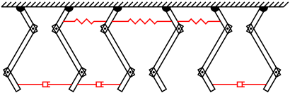
Figure 6: Uniformly coupled 3-link pendulums.

Corollary 4

Suppose ${\rm Re}\,\lambda_{2}(\ell_{\rm d}+j\ell_{\rm r})>0$ and both $(C_{\rm d},\,M^{-1}K)$ and $(C_{\rm r},\,M^{-1}K)$ are observable pairs. Then there exists $r>0$ such that the array (46) synchronizes for all $\varepsilon\in(0,\,r)$.

Proof. We begin by proving the implication

$${\rm Re}\,\lambda_{2}(\ell_{\rm d}+j\ell_{\rm r})>0\quad\implies\quad{\rm Re}\,\lambda_{2}(\alpha\ell_{\rm d}+j\beta\ell_{\rm r})>0\ \ \mbox{for all scalars}\ \ \alpha,\,\beta>0\,.$$ (47)

Given $\alpha,\,\beta>0$, consider the matrix $\alpha\ell_{\rm d}+j\beta\ell_{\rm r}$. Note that $\ell_{\rm d},\,\ell_{\rm r}\geq 0$ thanks to $\ell_{\rm d},\,\ell_{\rm r}\in\mathcal{L}(q,\,1)$. Therefore all the eigenvalues of $\alpha\ell_{\rm d}+j\beta\ell_{\rm r}$ are on the closed right half plane by Fact 1. Also, since $\ell_{\rm d}{\mathbf{1}}_{q}=0$ and $\ell_{\rm r}{\mathbf{1}}_{q}=0$, we have $(\alpha\ell_{\rm d}+j\beta\ell_{\rm r}){\mathbf{1}}_{q}=0$. Hence, without loss of generality, we can let $\lambda_{1}(\alpha\ell_{\rm d}+j\beta\ell_{\rm r})=0$. Consider now the situation ${\rm Re}\,\lambda_{2}(\alpha\ell_{\rm d}+j\beta\ell_{\rm r})\leq 0$. This implies $\lambda_{2}(\alpha\ell_{\rm d}+j\beta\ell_{\rm r})=j\gamma$ for some $\gamma\in{\mathbb{R}}$. Let $\xi_{2}\in{\mathbb{C}}^{q}$ be the corresponding unit eigenvector:

$$(\alpha\ell_{\rm d}+j\beta\ell_{\rm r})\xi_{2}=j\gamma\xi_{2}\,.$$ (48)

If $j\gamma\neq 0$ then clearly we must have $\xi_{2}\notin{\rm span}\,\{{\mathbf{1}}_{q}\}$. If $j\gamma=0$, on the other hand, then we can choose $\xi_{2}\notin{\rm span}\,\{{\mathbf{1}}_{q}\}$. For if we could not then ${\mathbf{1}}_{q}$ would have to be the only eigenvector for the repeated eigenvalue at the origin. This would require that there existed a generalized eigenvector $\zeta$ satisfying $(\alpha\ell_{\rm d}+j\beta\ell_{\rm r})\zeta={\mathbf{1}}_{q}$ which, because $\alpha\ell_{\rm d}+j\beta\ell_{\rm r}$ is symmetric, would lead to the following contradiction

$$1={\mathbf{1}}_{q}^{T}{\mathbf{1}}_{q}={\mathbf{1}}_{q}^{T}(\alpha\ell_{\rm d}+j\beta\ell_{\rm r})\zeta=((\alpha\ell_{\rm d}+j\beta\ell_{\rm r}){\mathbf{1}}_{q})^{T}\zeta=0\,.$$

Hence we let $\xi_{2}\notin{\rm span}\,\{{\mathbf{1}}_{q}\}$. Now, left-multiplying (48) by $\xi^{*}_{2}$ yields $\alpha\xi^{*}_{2}\ell_{\rm d}\xi_{2}+j\beta\xi^{*}_{2}\ell_{\rm r}\xi_{2}=j\gamma$ implying $\xi^{*}_{2}\ell_{\rm d}\xi_{2}=0$. This in turn gives us $\ell_{\rm d}\xi_{2}=0$ because $\ell_{\rm d}\geq 0$. Therefore we have to have $\ell_{\rm r}\xi_{2}=(\gamma/\beta)\xi_{2}$ by (48). Consequently, $(\ell_{\rm d}+j\ell_{\rm r})\xi_{2}=j(\gamma/\beta)\xi_{2}$. We also have $(\ell_{\rm d}+j\ell_{\rm r}){\mathbf{1}}_{q}=0$. Since $\xi_{2}$ and ${\mathbf{1}}_{q}$ are linearly independent, this means $\ell_{\rm d}+j\ell_{\rm r}$ has at least two eigenvalues on the imaginary axis. Therefore we have established ${\rm Re}\,\lambda_{2}(\alpha\ell_{\rm d}+j\beta\ell_{\rm r})\leq 0\implies{\rm Re}\,\lambda_{2}(\ell_{\rm d}+j\ell_{\rm r})\leq 0$, which gives us (47) because $\alpha,\,\beta$ were arbitrary.

Recall that $v_{1},\,v_{2},\,\ldots,\,v_{n}$ are the eigenvectors of $P=M^{-1/2}KM^{-1/2}$, the corresponding eigenvalues being $\sigma_{1},\,\sigma_{2},\,\ldots,\,\sigma_{n}$. Define now the vectors $\tilde{v}_{k}=M^{-1/2}v_{k}$. These $\tilde{v}_{k}$ are the eigenvectors of $M^{-1}K$ because we can write

$$M^{-1}K\tilde{v}_{k} = M^{-1}KM^{-1/2}v_{k}$$

$$= M^{-1/2}(M^{-1/2}KM^{-1/2}v_{k})$$

$$= M^{-1/2}(\sigma_{k}v_{k})$$

$$= \sigma_{k}\tilde{v}_{k}\,.$$

Define $\alpha_{k}=\|C_{\rm d}\tilde{v}_{k}\|^{2}$ and $\beta_{k}=\|C_{\rm r}\tilde{v}_{k}\|^{2}$ for $k=1,\,2,\,\ldots,\,n$. Recall $D_{ij}=d_{ij}C_{\rm d}^{T}C_{\rm d}$ and $R_{ij}=r_{ij}C_{\rm r}^{T}C_{\rm r}$. Starting from (28) we can write

$$G_{kk} = {\rm lap}\,(v_{k}^{T}M^{-1/2}D_{ij}M^{-1/2}v_{k})_{i,j=1}^{q}$$

$$= {\rm lap}\,(\tilde{v}_{k}^{T}C_{\rm d}^{T}C_{\rm d}\tilde{v}_{k}d_{ij})_{i,j=1}^{q}$$

$$= \|C_{\rm d}\tilde{v}_{k}\|^{2}{\rm lap}\,(d_{ij})_{i,j=1}^{q}$$

$$= \alpha_{k}\ell_{\rm d}\,.$$

Likewise, we have $B_{kk}=\beta_{k}\ell_{\rm r}$. Hence, for all $k=1,\,2,\,\ldots,\,n$,

$$G_{kk}+jB_{kk}=\alpha_{k}\ell_{\rm d}+j\beta_{k}\ell_{\rm r}\,.$$ (49)

Suppose now ${\rm Re}\,\lambda_{2}(\ell_{\rm d}+j\ell_{\rm r})>0$ and both $(C_{\rm d},\,M^{-1}K)$ and $(C_{\rm r},\,M^{-1}K)$ are observable pairs. By PBH observability condition [6] we have to have $C_{\rm d}\tilde{v}_{k}\neq 0$ and $C_{\rm r}\tilde{v}_{k}\neq 0$ for all $k=1,\,2,\,\ldots,\,n$. This means $\alpha_{k},\,\beta_{k}>0$. The result then follows by (47), (49), and Theorem 2.   $\blacksquare$

5 Pure dissipative coupling

In the last part of our analysis we dispense with the restorative coupling (e.g., springs connecting the pendulums) altogether and focus on the special case of (2) where all $R_{ij}=0$. This is the case where the coupling is purely dissipative:

$$M{\ddot{x}}_{i}+Kx_{i}+\sum_{j=1}^{q}D_{ij}({\dot{x}}_{i}-{\dot{x}}_{j})=0\,,\qquad i=1,\,2,\,\ldots,\,q\,.$$ (50)

The next result is closely related to [17, Cor. 1].

Theorem 3

The array (50) synchronizes if and only if $\lambda_{2}(G_{kk})>0$ for all $k=1,\,2,\,\ldots,\,n$.

Proof. Define the matrix $\Omega_{0}=G+j[\Lambda\otimes I_{q}]$. Note that the array (50) synchronizes if and only if ${\rm Re}\,\lambda_{n+1}(\Omega_{0})>0$ thanks to Remark 1. Some of our earlier arguments on $\Omega_{\varepsilon}$ are valid also on $\Omega_{0}$. By those arguments we see that $\Omega_{0}[e_{k}\otimes{\mathbf{1}}_{q}]=j\sigma_{k}[e_{k}\otimes{\mathbf{1}}_{q}]$ for $k=1,\,2,\,\ldots,\,n$. That is, each $[e_{k}\otimes{\mathbf{1}}_{q}]$ is an eigenvector, the corresponding eigenvalue being $j\sigma_{k}$. Also, all the eigenvalues of $\Omega_{0}$ are on the closed right half plane by Fact 1. Therefore we can let, without loss of generality, $\lambda_{k}(\Omega_{0})=j\sigma_{k}$ for $k=1,\,2\,\ldots,\,n$.

Suppose the array (50) fails to synchronize. This implies $\lambda_{n+1}(\Omega_{0})=j\beta$ for some $\beta\in{\mathbb{R}}$. Let $\xi\in({\mathbb{C}}^{q})^{n}$ be the corresponding unit eigenvector. We can write $j\beta=\xi^{*}G\xi+j\xi^{*}[\Lambda\otimes I_{q}]\xi$ by (4). This tells us (since $G\geq 0$ and $[\Lambda\otimes I_{q}]>0$) that $\xi^{*}G\xi=0$ and, consequently, $G\xi=0$. Therefore $[\Lambda\otimes I_{q}]\xi=\beta\xi$. That is, $\xi$ is an eigenvector of $[\Lambda\otimes I_{q}]$ and $\beta$ an eigenvalue. Now, $\Lambda={\rm diag}\,(\sigma_{1},\,\sigma_{2},\,\ldots,\,\sigma_{n})$ implies $\beta\in\{\sigma_{1},\,\sigma_{2},\,\ldots,\,\sigma_{n}\}$. Without loss of generality let us take $\beta=\sigma_{1}$. Then $\xi$ has to have the form $\xi=[e_{1}\otimes w]$ for some $w\in{\mathbb{C}}^{q}$. Again without loss of generality we can further assume $w\notin{\rm span}\,\{{\mathbf{1}}_{q}\}$. Generality is not lost; for, otherwise, $[e_{1}\otimes{\mathbf{1}}_{q}]$ would be the only eigenvector of $\Omega_{0}$ for the repeated eigenvalue $j\sigma_{1}$, which would require the existence of a generalized eigenvector $\zeta$ satisfying $(\Omega_{0}-j\sigma_{1}I_{qn})\zeta=[e_{1}\otimes{\mathbf{1}}_{q}]$. This however yields the contradiction below because $\Omega_{0}^{T}=\Omega_{0}$

$$1=[e_{1}\otimes{\mathbf{1}}_{q}]^{T}[e_{1}\otimes{\mathbf{1}}_{q}]=[e_{1}\otimes{\mathbf{1}}_{q}]^{T}(\Omega_{0}-j\sigma_{1}I_{qn})\zeta=((\Omega_{0}-j\sigma_{1}I_{qn})[e_{1}\otimes{\mathbf{1}}_{q}])^{T}\zeta=0\,.$$

Note that we have

$$w^{*}G_{11}w=[e_{1}\otimes w]^{*}G[e_{1}\otimes w]=\xi^{*}G\xi=0$$

implying $G_{11}w=0$ because $G_{11}\geq 0$ thanks to $G_{11}\in\mathcal{L}(q,\,1)$ by Lemma 3. Furthermore, $G_{11}{\mathbf{1}}_{q}=0$. Since the set $\{w,\,{\mathbf{1}}_{q}\}$ is linearly independent the eigenvalue of $G_{11}$ at the origin must be repeated. This means $\lambda_{2}(G_{11})=0$ because $G_{11}\geq 0$.

To show the other direction let us suppose this time that $\lambda_{2}(G_{\ell\ell})\leq 0$ for some $\ell$. Being a Laplacian matrix, $G_{\ell\ell}\geq 0$ and $G_{\ell\ell}{\mathbf{1}}_{q}=0$. Therefore the eigenvalue at the origin is repeated and there exists a vector $u\notin{\rm span}\,\{{\mathbf{1}}_{q}\}$ satisfying $G_{\ell\ell}u=0$. Construct now the vector $\eta=[e_{\ell}\otimes u]$. Clearly, this vector satisfies

$$\eta\notin{\rm span}\,\{[e_{1}\otimes{\mathbf{1}}_{q}],\,[e_{2}\otimes{\mathbf{1}}_{q}],\,\ldots,\,[e_{n}\otimes{\mathbf{1}}_{q}]\}\,.$$ (51)

Moreover,

$$\eta^{*}G\eta=[e_{\ell}\otimes u]^{*}G[e_{\ell}\otimes u]=u^{*}G_{\ell\ell}u=0$$

which, since $G\geq 0$, implies $G\eta=0$. This allows us to see that $\eta$ is an eigenvector of $\Omega_{0}$ because

$$\Omega_{0}\eta = (G+j[\Lambda\otimes I_{q}])\eta$$ (52)

$$= j[\Lambda\otimes I_{q}][e_{\ell}\otimes u]$$

$$= j[(\Lambda e_{\ell})\otimes(I_{q}u)]$$

$$= j[(\sigma_{\ell}e_{\ell})\otimes(I_{q}u)]$$

$$= j\sigma_{\ell}[e_{\ell}\otimes u]$$

$$= j\sigma_{\ell}\eta\,.$$

Now, (51) and (52) tell us that $\Omega_{0}$ has at least $n+1$ linearly independent eigenvectors whose eigenvalues lie on the imaginary axis. But this implies ${\rm Re}\,\lambda_{n+1}(\Omega_{0})=0$. Hence the result.   $\blacksquare$

Consider now the scenario where the coupling in the array (50) is uniform. That is, there exists a matrix $C_{\rm d}\in{\mathbb{R}}^{m_{\rm d}\times n}$ such that $D_{ij}=d_{ij}C_{\rm d}^{T}C_{\rm d}$ where $d_{ij}$ are nonnegative scalars. Under this condition the array dynamics take the form

$$M{\ddot{x}}_{i}+Kx_{i}+\sum_{j=1}^{q}d_{ij}C_{\rm d}^{T}C_{\rm d}({\dot{x}}_{i}-{\dot{x}}_{j})=0\,,\qquad i=1,\,2,\,\ldots,\,q\,.$$ (53)

The coupling of this array is represented by two parameters: the Laplacian matrix $\ell_{\rm d}={\rm lap}\,(d_{ij})_{i,j=1}^{q}$ and the output matrix $C_{\rm d}$. How they are linked to synchronization is stated next.

Corollary 5

The array (53) synchronizes if and only if $\lambda_{2}(\ell_{\rm d})>0$ and $(C_{\rm d},\,M^{-1}K)$ is observable.

Proof. The demonstration is similar to that of Corollary 4.   $\blacksquare$

6 Conclusion

In this paper we studied the problem of synchronization in an array of identical oscillators subject to both dissipative and restorative coupling. We presented a simple way to combine the pair of matrix-weighted Laplacians (one representing the dissipative, the other the restorative coupling) in a single complex-valued matrix and established an equivalence relation between a certain spectral property of this matrix and the collective behavior of the oscillators. Also, we projected this method to generate more refined conditions for synchronization applicable when the restorative coupling is either weak or absent altogether.