Energy-based Tuning of Convolutional Neural Networks on Multi-GPUs

Abstract

Deep Learning (DL) applications are gaining momentum in the realm of Artificial Intelligence, particularly after GPUs have demonstrated remarkable skills for accelerating their challenging computational requirements. Within this context, Convolutional Neural Network (CNN) models constitute a representative example of success on a wide set of complex applications, particularly on datasets where the target can be represented through a hierarchy of local features of increasing semantic complexity. In most of the real scenarios, the roadmap to improve results relies on CNN settings involving brute force computation, and researchers have lately proven Nvidia GPUs to be one of the best hardware counterparts for acceleration. Our work complements those findings with an energy study on critical parameters for the deployment of CNNs on flagship image and video applications: object recognition and people identification by gait, respectively. We evaluate energy consumption on four different networks based on the two most popular ones (ResNet/AlexNet): ResNet (167 layers), a 2D CNN (15 layers), a CaffeNet (25 layers) and a ResNetIm (94 layers) using batch sizes of 64, 128 and 256, and then correlate those with speed-up and accuracy to determine optimal settings. Experimental results on a multi-GPU server endowed with twin Maxwell and twin Pascal Titan X GPUs demonstrate that energy correlates with performance and that Pascal may have up to 40% gains versus Maxwell. Larger batch sizes extend performance gains and energy savings, but we have to keep an eye on accuracy, which sometimes shows a preference for small batches. We expect this work to provide a preliminary guidance for a wide set of CNN and DL applications in modern HPC times, where the GFLOPS/w ratio constitutes the primary goal.

1 Introduction

We are witnessing a revolution in computer vision with the advent of Deep Learning (DL) architectures [1]. Computer vision problems have been traditionally solved using hand-crafted features specifically designed to tackle particular problems [2, 3, 4, 5], where the main challenge was to find the right descriptors for certain image contents. DL introduced a general way to proceed via supervised learning. Fukushima et al.  [6] were pioneers developing a hierarchical architecture for handwritten character recognition and other pattern recognition, which we may consider the inspiration for Convolutional Neural Networks (CNNs).

In 1998, LeCun et al. [7] introduced one of the first and most popular architectures for handwritten character recognition, and a decade later, Serre et al.  [8] contributed with a new general framework for the recognition of complex visual scenes. Those first steps were based on a small number of layers and limited datasets due to the modest computational power available, so researchers often moved to less demanding approaches like SVM [9].

In 2012, Krizhevsky et al. [10] released ‘AlexNet’, a CNN composed of 25 layers and around 60 million parameters. GPUs were capable to train the model with CUDA in a reasonable amount of time using four GPUs, and since then, the fascinating evolution of GPU performance and its recent emphasis on DL has propelled those models to gain extraordinary popularity. Meanwhile, new datasets [11, 12, 13] containing millions of samples were released to train models with even more parameters without overfitting, promoting CNN models to be established as the state-of-art in computer vision. The challenge for researchers to tune computer vision applications at this point is no longer based on low-level features, but on general neural network components like number of layers, set of parameters or batch size. Within this trend, the last couple of years have been prolific in assorted areas like image recognition [14, 15], action recognition [16, 17], object detection [18, 19], and biometric identification [20, 21], just to mention a few akin to that of this work.

This trend has been lately fortified with the arrival of deep learning frameworks publicly available, like Caffe [22], TensorFlow [23], CNTK [24], MatConvNet [25] and PyTorch [26]. Most of these frameworks are optimized for GPUs and still require large execution times, so energy consumption on GPUs becomes critical. That way, the flagship metric is no longer GFLOPS (Giga Floating-Point Operations Per Second), but GFLOPS/w (GFLOPS per watt). This paper emphasizes energy over speed, choosing representative CNN instances to shed some light about the way energy is spent within CNN depending on its architecture (ResNet/CaffeNet/2D-CNN), input dataset (images/videos) and batch size (64/128/256). Finally, a correlation with performance and accuracy is performed to complete our analysis.

On the hardware side, latest generations of Nvidia GPUs, namely Maxwell (2014) and Pascal (2016), have been used for our experimental setup. Those two generations have contributed like no other before to optimize the GFLOPS/w ratio, and the advantage amplifies in supercomputers to populate the green500 list [27]. Our work gathers results combining the best GeForce model for those two generations, Titan X, and a multi-GPU server endowed with up to four GPUs, returning somehow to the departure point where AlexNet emerged five years ago.

Previous works have contributed with performance analysis of DL networks in GPU architectures  [28, 29, 30]. We extend those results to energy for a more complete study using a probe plugged to the GPU that measures power consumption at real-time for every stage a deep learning algorithm consists of. Major contributions of this paper on DL algorithms are the following:

• A combined energy and performance analysis on a multi-GPU setup using the two most popular types of CNNs, and particularized for the forward, backward and weight update stages of a DL algorithm.

• Accuracy statistics to find out the best algorithm parametrization depending on three different metrics: time, energy consumption and energy-delay product.

• Comparison between Maxwell and Pascal architectures for all those features above.

The rest of this paper is structured as follows. Section 2 introduces some related work. Section 3 provides a general overview of CNNs, and Section 4 particularizes our selection of CNNs for the experimental study. Section 5 outlines our CNN implementation on multi-GPU environments. Section 6 describes the infrastructure we have used for measuring energy on GPUs. Section 7 introduces the input datasets. Section 8 presents and discusses the experimental results, and finally, Section 9 summarizes the conclusions drawn from this work.

2 Related Work

Energy consumption has gained relevance among researchers during the big-data era, sometimes representing more than 20% of the budget in Data Centers nowadays. For an illustrative example, costs have exceeded 5 billion dollars per year over the last decade only in the US [31], and it is predicted that the energy billing will increase in forthcoming years if power optimizations are not conducted in all levels, including operating systems, kernels and applications.

The industry is aware about the need of low-power CNN acceleration when using them extensively. Google is a clear example with Tensor Processing Unit tailored to their TensorFlow framework in its data centers, claiming that they are able to reduce power an order of magnitude versus GPUs [32].

The research community is also helping to reduce power on CNNs. Five notable examples recently published in 2016-17 are the following:

• Moons et al. [33] propose methods at system and circuit level based on approximate computing. They always perform training using 32-bit, lowering precision during the test phase. They claim energy gains up to 30× without losing classification accuracy and more than 100× at 99% classification accuracy, compared to a commonly used 16-bit fixed point number format.

• Cai et al. propose NeuralPower [34], a layer-wise predictive framework based on sparse polynomial regression, for predicting the serving energy consumption of a CNN deployed on different GPU platforms and Deep Learning software tools, attaining an average accuracy of 88.24% in execution time, 88.34% in power, and 97.21% in energy.

• Andri et al. introduce YodaNN [35], an energy and area efficiency accelerator based on ASIC hardware optimized for BinaryConnect CNNs which basically removes the need for expensive multiplications during training, also reducing I/O bandwidth and storage.

• Yang et al. [36] propose an energy-aware pruning algorithm for CNNs that directly uses energy consumption estimation of a CNN to guide the pruning process. The energy consumption of AlexNet and GoogLeNet are reduced by 3.7x and 1.6x, respectively, with less than 1% top-5 accuracy loss. Results are obtained via a energy estimation tool for Deep Neural Networks publicly available in [37].

• Lin et al. [38] propose PredictiveNet to skip a large fraction of convolutions in CNNs at runtime without modifying the CNN structure or requiring additional branch networks. An analysis supported by simulations is provided to justify how to preserve the mean square error (MSE) of the nonlinear layer outputs. Energy savings are attained by reducing the computational cost by a factor of 2.9× compared to a state-of-the-art CNN, while incurring marginal accuracy degradation.

Moving away from estimators, predictors and simulators, we may find examples of real energy measurements and studies on low-power devices like DSPs [39] and FPGAs [40], even for CNN applications [41, 42]. But to the best of our knowledge, our work is pioneer on measuring the actual power consumption of CNNs with wires and measurement devices physically plugged to the pinout of latest GPU generations and multi-GPU platforms, and even identifying the most expensive operators and functions in terms of energy budget.

3 CNN Overview

Convolutional Neural Networks (CNNs) are a type of neural network particularly successful on computer vision problems where the information is spatially related and it can be represented in a hierarchical mode [1]. A CNN is defined by its architecture which is a set several convolutional layers and several fully connected layers. Each convolutional layer is, in general, the composition of a non-linear (convolutional filter) layer and a pooling or sub-sampling layer to get some spatial invariance.

In the last years, CNN models are standing out above on a wide range of applications, like object detection, text classification, natural language processing or scene labeling [10, 43, 44, 45]. CNNs are specially successful on data where the target can be represented with a feature hierarchy of increasing semantic complexity. When successfully trained, the output of the last hidden layer can be seen as the representation of the target in a high-level space. The fully connected layers reduce the dimensionality of the representation and hold the high-level knowledge, improving the classification accuracy.

During training, a random batch, which is a set of $N$ samples, is selected from the training samples and passed through the model obtaining the activations (outputs) of each layer and the final output. This final output, depending on the type of application, can be a probability distribution (classification), an image (segmentation), a number (regression), etc. With this final output and its corresponding ground-truth label, a loss function designed for each problem computes the error, which is back-propagated from the top layers to the bottom ones.

Therefore, during training, there are three different processes in a CNN:

1. Forward, where a batch is passed through the CNN to obtain the activations.

2. Backward, where the error is back-propagated to obtain the derivatives.

3. Weights update, for the weights of the model to be updated according to the solver. This stage is negligible compared to the previous two and we have preferred to discard it for the sake of simplicity.

During test, only the forward process is executed to obtain the final output of the model. Along with the back-propagation process, each layer computes its own derivatives according to the error coming from the top layer. Once derivatives are computed, the average derivative from the $N$ samples is computed and the weights of the model are updated according to the solver selected, with the Stochastic Gradient Descent (SGD) being the most common case.

These three steps are repeated for $M$ epochs until the algorithm converges, with an epoch being a set of $M_{b}$ batches (or iterations) to process the whole training set. For example, in a training set composed of 1000 samples and batches of 100 samples, an epoch would have 10 batches or iterations.

This work focuses on energy consumption and execution time of the forward and backward processes, also analyzing the global accuracy for the model. Energy, acceleration and precision are put in perspective on modern GPUs as attractive candidates for a leadership on different models and problems, among which we select a bunch of popular instances for a representative case study.

4 Our CNN Selection for Power Analysis

We select two popular CNN architectures typically applied to process input data in computer vision, either using images or videos. On the image side, we deal with image recognition, that is, identify what appears in an image; whereas using videos we focus on gait, that is, the challenge of identifying people by the way they walk. We pretend this way to explore setups acting as solid templates for deep learning in computer vision, so that conclusions can easily be extrapolated to a wide range of problems.

The energy consumed by an algorithm is directly proportional to the number of operations and its type. In a CNN, this type is defined by the architecture and the kind of layers. The architecture also plays an important role on the number of operations, because that number increases with the number of layers. In addition, during training, more than one sample is passed through the CNN according to the mini-batch training process, and so the number of samples (batch size) influences power consumption and the convergence process in a decisive manner.

Each layer has its own number and type of operations, so we now characterize the most common layers used in the majority of CNNs. For simplicity, all formulas are related to a single sample as input. Thus, when dealing with a batch, expressions must be multiplied by the batch size.

We start introducing some terminology:

• $w_{in},h_{in}$. Width and height of the input sample, respectively.

• $w_{out},h_{out}$. Width and height of the output sample, respectively.

• $ch_{in},ch_{out}$. Number of input and output channels, respectively.

• $k_{w},k_{h}$. Kernel width and height, respectively.

The terms $w_{out}$ and $h_{out}$ are obtained from the formula $w_{out}=\frac{(w_{in}-k_{w})+2P}{S}$, with $P$ being the padding applied to the input and $S$ the stride or step of the kernel. Similarly, $h_{out}=\frac{(h_{in}-k_{h})+2P}{S}$.

Using previous definitions, the functionality and number of operations performed at each layer are shown as follows.

Convolution. It applies a kernel to the input sample. The number of operations is defined on Eq. 1. In this layer, the type of operation is multiply–accumulate (macc). In addition, if the convolution has bias, we need to include $ch_{out}$ add operations.

$$\#operations=(k_{w}\cdot k_{h})(w_{out}\cdot h_{out})\cdot ch_{in}\cdot ch_{out}$$ (1)

Fully connected. It has full connections to all activations in the previous layer. The number of operations is defined on Eq. 2. In this case, the type of operation is multiply–accumulate (macc).

$$\#operations=(w_{in}\cdot h_{in})\cdot ch_{in}\cdot ch_{out}$$ (2)

Pooling. It reduces the spatial size of the input to lower the amount of parameters and computation in the network. The number of operations is defined on Eq. 3. The type of operation depends on the architecture, being max the most common one.

$$\#operations=(k_{w}\cdot k_{h})(w_{out}\cdot h_{out})\cdot ch_{in}$$ (3)

ReLU. It applies a regularization function to the input. The number of operations is defined on Eq. 4. In this case, the type of operation is max.

$$\#operations=(w_{in}\cdot h_{in})\cdot ch_{in}$$ (4)

Dropout. It randomly disconnects inputs to minimize overfitting. The number of operations is defined on Eq. 5. In this case, the type of operation is multiplication by $0$ or $1$ depending on the the input to be disconnected or not.

$$\#operations=(w_{in}\cdot h_{in})\cdot ch_{in}$$ (5)

Batch normalization. It normalizes the input subtracting the mean and dividing by the standard deviation. The number of operations is defined on Eq. 6. The type of operations are add and division. As the number of both operations is the same, we combine them into a single equation.

$$\#operations=(w_{in}\cdot h_{in})\cdot ch_{in}\cdot 2$$ (6)

Softmax. It scales a $K-$dimensional vector of arbitrary real values to a $K-$dimensional vector of real values in the range $[0,1]$ that add up to $1$. The number of operations is defined on Eq. 7. The type of operations are exponential, add and division. As the number of the three operations is the same, we combine them into a single equation.

$$\#operations=(w_{in}\cdot h_{in})\cdot ch_{in}\cdot 3$$ (7)

Apart from the number and type of operations, each layer is also characterized by the data volume read and written. In this analysis, the formulas are valid for all layers so we present a formula for the reading process 8 and another one for the writing one 9. Note that in the reading part, the second term refers to the weights of the layer.

$$read=(w_{in}\cdot h_{in})\cdot ch_{in}+(k_{w}\cdot k_{h})\cdot ch_{in}$$ (8)

$$written=(w_{out}\cdot h_{out})\cdot ch_{out}$$ (9)

For building our benchmark, we first select four architectures: (1) a 2D-CNN [46] based on AlexNet [10] using videos as inputs, (2) a ResNet network [47] specifically developed for gait recognition [21] involving videos, (3) CaffeNet, which is an implementation of AlexNet released with Caffe, and (4) ResNetIm, which is the ResNet34 published in [47]. Then, for each architecture, we select three batch sizes so that we can characterize the energy consumed and accuracy depending on networks and batch sizes.

Among those hyper-parameters to be optimized within a DL network, we have selected the one which has a bigger impact in performance and accuracy. Other candidates might be the learning rate, to affect the convergence speed, and the stride of the convolutions, which defines the step size of the convolutions applied to an image. The learning rate only affects if a good value is known beforehand to guarantee a fast convergence, but in most cases that value is a heuristic determined through an exhaustive experimental process. The stride has a huge impact in the performance and energy (less operations are performed with higher stride values), and also in the model, because networks can lose important local information. Nevertheless, latest networks like ResNet just use stride one and small convolutions to capture that information, leaving this hyper-parameter with a minor influence and highly sensitive to the problem itself.

4.1 Architecture analysis

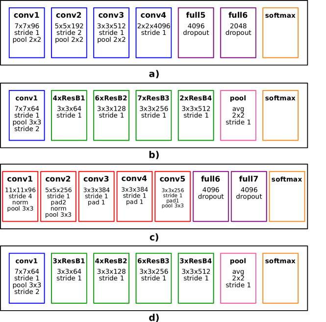
Figure 1: Proposed CNN models for gait signature extraction. a) 2D-CNN: linear CNN with four 2D convolutions, two fully connected layers and a softmax classifier. b) ResNet: residual CNN with a 2D convolution, four residual blocks, an average pooling layer and a final softmax classifier. Note that before the first block of each kind (ResB 1, 2, 3, 4), there is an adapter convolution to resize the input image to that of the next block. c) CaffeNet: linear CNN with five 2D convolutions, two fully connected layers and a softmax classifier. d) ResNetIm: residual CNN with a 2D convolution, four residual blocks, an average pooling layer and a final softmax classifier. Note that before the first block of each kind (ResB 1, 2, 3, 4), there is an adapter convolution to resize the input image to that of the next block.

2D-CNN (15 layers).

This architecture is inspired by AlexNet [10] and it is adapted to the specific requirements of gait recognition. For our particular case, we use optical flow as input following the approach described in [46].

The proposed CNN comprises the following sequence of layers (see Fig. 1.a):

1. ‘conv1’, 96 filters of size $7\times 7$ applied with stride 1 followed by max pooling $2\times 2$.

2. ‘conv2’, 192 filters of size $5\times 5$ applied with stride 2 followed by max pooling $2\times 2$.

3. ‘conv3’, 512 filters of size $3\times 3$ applied with stride 1 followed by max pooling $2\times 2$.

4. ‘conv4’, 4096 filters of size $2\times 2$ applied with stride 1.

5. ‘full5’, fully-connected layer with 4096 units and dropout.

6. ‘full6’, fully-connected layer with 2048 units and dropout.

7. ‘softmax’, softmax layer with as many units as subject identities.

ResNet (167 layers).

This CNN is composed of a sequence of layers and residual blocks shown in Fig. 1.b (two consecutive convolutions of size $3\times 3$ plus a sum layer, as defined in [47]). The main blocks in our model are:

1. ‘conv1’, 64 filters of size $7\times 7$ applied with stride 1 followed by max pooling $3\times 3$ with stride 2.

2. ‘4xResB1’, 4 residual blocks with convolutions of 64 filters of size $3\times 3$ applied with stride 1.

3. ‘6xResB2’, 6 residual blocks with convolutions of 128 filters of size $3\times 3$ applied with stride 1.

4. ‘7xResB3’, 7 residual blocks with convolutions of 256 filters of size $3\times 3$ applied with stride 1.

5. ‘2xResB4’, 2 residual blocks with convolutions of 512 filters of size $3\times 3$ applied with stride 1.

6. ‘pool’, global average pooling $2\times 2$.

7. ‘softmax’, softmax layer with as many units as subject identities.

CaffeNet (25 layers).

This architecture is inspired by AlexNet [10], and it was released within Caffe, to be used for object recognition in images. The input has a size of $227\times 227$, obtained from a random crop of the original images resized to $256\times 256$.

The proposed CNN is composed by the following sequence of layers (see Fig. 1.c):

1. ‘conv1’, 96 filters of size $11\times 11$ applied with stride 4 followed by max pooling $3\times 3$ and a normalization layer of size $5\times 5$.

2. ‘conv2’, 256 filters of size $5\times 5$ applied with stride 1 and padding 2 followed by max pooling $3\times 3$ and a normalization layer of size $5\times 5$.

3. ‘conv3’, 384 filters of size $3\times 3$ applied with stride 1 and padding 1.

4. ‘conv4’, 384 filters of size $3\times 3$ applied with stride 1 and padding 1.

5. ‘conv5’, 256 filters of size $3\times 3$ applied with stride 1 and padding 1 followed by max pooling $3\times 3$.

6. ‘full6’, fully-connected layer with 4096 units and dropout.

7. ‘full7’, fully-connected layer with 4096 units and dropout.

8. ‘softmax’, softmax layer with as many units as object identities.

ResNetIm (94 layers).

This CNN is composed of a sequence of layers and residual blocks shown in Fig. 1.d (two consecutive convolutions of size $3\times 3$ plus a sum layer, as defined in [47]). The main blocks in our model are:

1. ‘conv1’, 64 filters of size $7\times 7$ applied with stride 1 followed by max pooling $3\times 3$ with stride 2.

2. ‘3xResB1’, 3 residual blocks with convolutions of 64 filters of size $3\times 3$ applied with stride 1.

3. ‘4xResB2’, 4 residual blocks with convolutions of 128 filters of size $3\times 3$ applied with stride 1.

4. ‘6xResB3’, 6 residual blocks with convolutions of 256 filters of size $3\times 3$ applied with stride 1.

5. ‘3xResB4’, 3 residual blocks with convolutions of 512 filters of size $3\times 3$ applied with stride 1.

6. ‘pool’, global average pooling $2\times 2$.

7. ‘softmax’, softmax layer with as many units as subject identities.

The convolutional layers from all CNNs use the rectification (ReLU) activation function. Applying the formulas of Section 4 to characterize our networks, we may obtain the number of arithmetic operations and memory accesses required, which are compiled in Table 1. In addition, we show the Computation to Communication ratio [48] defined as: $CTC=\frac{N_{op}}{N_{d}}$ where $N_{op}$ is the total number of operations and $N_{d}$ is the amount of data read.

Table 1: Characterization of our CNN networks through number of arithmetic operations, data volume read and written per sample during forward step and ratio between the number of operations and amount of data read.

Type of CNN	# arithmetic operations	Data volume read	Data volume written	CTC ratio
ResNet	425.13M	87.6 MB	4.8 MB	18.5
2D-CNN	783.84M	73.8 MB	1.9 MB	40.5
CaffeNet	727.20M	239.1 MB	6 MB	11.6
ResNetIm	2080.96M	97.1 MB	46.6 MB	81.8

4.2 Batch analysis

The batch size (number of samples) used during training influences three aspects of the model: number of operations, performance and accuracy. More precisely, the number of operations is defined by the Eq. 10 and the data read and written by Eq. 11 and 12 respectively.

$$\#operations=B\cdot operationsSample$$ (10)

$$readB=B\cdot readSample$$ (11)

$$writtenB=B\cdot writtenSample$$ (12)

where $B$ represents the batch size, $operationsSample$ the number of operations, $readSample$ the data read and $writtenSample$ the data written, obtained by the formulas described in Section 4 for one sample.

The batch size defines the number of samples used as input to a model. Therefore, the bigger the batch size, the more number of operations performed as there are more samples to process. If we consider the latency due to input data coming from secondary memory, a bigger batch size allows a better overlapping between computations on GPU and CPU to GPU communications. Moreover, we have to remember that the batch size plays an important role during training as the weights are updated according to the mean of the gradients obtained from the images of the batch. Therefore, there is a trade off here: bigger batches improve accuracy in gradients, but smaller batches (noisy gradients) benefit convergence as it maximizes the exploration of the solution space. Taking into account all these considerations, we are going to evaluate three batch sizes: 64, 128 and 256. These values are the most common in the literature and they achieve good results in terms of accuracy for the problems tested here, and constitute the best candidates in our quest for the optimal batch size in terms of accuracy, performance and power requirements.

4.3 Energy measurement

The training process is composed of three main parts, namely, forward, backward and weight updating (see Section 3). According to our experiments, forward and backward steps consume on average more than $95\%$ of the execution time. Then, we focus on the two first steps to simplify our analysis. In any case, total values can always be roughly obtained by adding this percentage to the sum of forward and backward steps.

Algorithm 1 shows the training process and the points established for measurements. Since the algorithm executes concurrently on the GPU, we use CUDA events to make sure that the measured execution is over. Also, our infrastructure for measuring power is attached to a single GPU, which means that on multi-GPU executions, we nominate a root GPU and the global consumption is extrapolated for the set involved. More details are provided later in Section 5. Note that $maxIter$ is computed as the number of iterations in an epoch multiplied by the number of epochs.

  model = InitializeModel()

  iter = 0

  maxIter = Initialize(InitParams)

  while iter $<$ maxIter do

     StartTimer()

     data = LoadData(batch)

     time = StopTimer()

     StartTimerAndPowerMeassurement()

     output = Forward(model, data)

     time, power = StopTimerAndPowerMeassurement()

     StartTimerAndPowerMeassurement()

     derivatives = Backward(model, output)

     time, power = StopTimerAndPowerMeassurement()

     model = updateWeights(model, derivatives)

     iter++

  end while

Algorithm 1 Schematic for CNN training.

5 GPU Implementation

We use Caffe [22] (commit c98de53b7817c732b482c2fa810f09c260c58857) with cuDNN [49] 6.0, NCCL 2.1.2 and CUDA 8.0 libraries to train our CNNs. Forward and backward processes are entirely implemented in GPU by Caffe using the primitives available in cuDNN. To update the weights efficiently in a multi-GPU environment, Caffe uses primitives included in NCCL. Finally, the CPU just loads the input data.

When the model is being trained on a single GPU, we use a CPU thread to load data constantly from secondary storage into a CPU memory buffer. This way, we maximize overlapping between data transfers and GPU computation. If there is enough data to fill a batch, the GPU computes the forward and backward steps while the CPU is loading new data. Finally, the weights are updated in the GPU and the process starts again to compute a new batch.

When the model is being trained using multiple GPUs, each GPU has a CPU thread which is loading data into its own memory buffer, thus, we have one thread and one memory buffer per GPU. In this case, each GPU has exactly the same CNN architecture model with similar weights, but the batch is divided among GPUs (e.g. a batch with 64 samples trained with 2 GPUs is splitted into 2 sub-batches of 32 samples). Once all GPUs have finished their computation, the derivatives are collected and the weights updating process starts. In order to optimize the weights updating step, Caffe uses the ncclAllReduce primitive, which gathers local gradients, computes global derivatives and leaves a copy of those on each GPU. It is important to clarify that according to the documentation, Caffe uses a tree reduction strategy , but recent implementations use NCCL instead to improve the multi-GPU performance. Thus, ncclAllReduce arranges the GPUs in a virtual ring and the information to be transferred is split into small packages. Then, the $i$-th GPU transfers a package to its neighbour ($i+1$) and, at the same time, performs the reduction computation with the information coming from the $(i-1)$-th GPU. This process is repeated until all packages are transferred and all reductions are done. When the primitive ends, all GPUs store the same information, that is, the values of global derivatives. That way, each GPU updates the model independently.

6 Monitoring Energy

6.1 Measurement Infrastructure

We have built a system to measure current, voltage and wattage based on a Beaglebone Black, an open-source hardware [50] combined with the Accelpower module [51], which has eight INA219 sensors [52]. Inspired by [53], wires taken into account are two power pins on the PCI-express slot (12 and 3.3 volts) plus six external 12 volt pins coming from the power supply unit (PSU) in the form of two supplementary 6-pin connectors (half of the pins used for grounding). See Figure 2 for details.

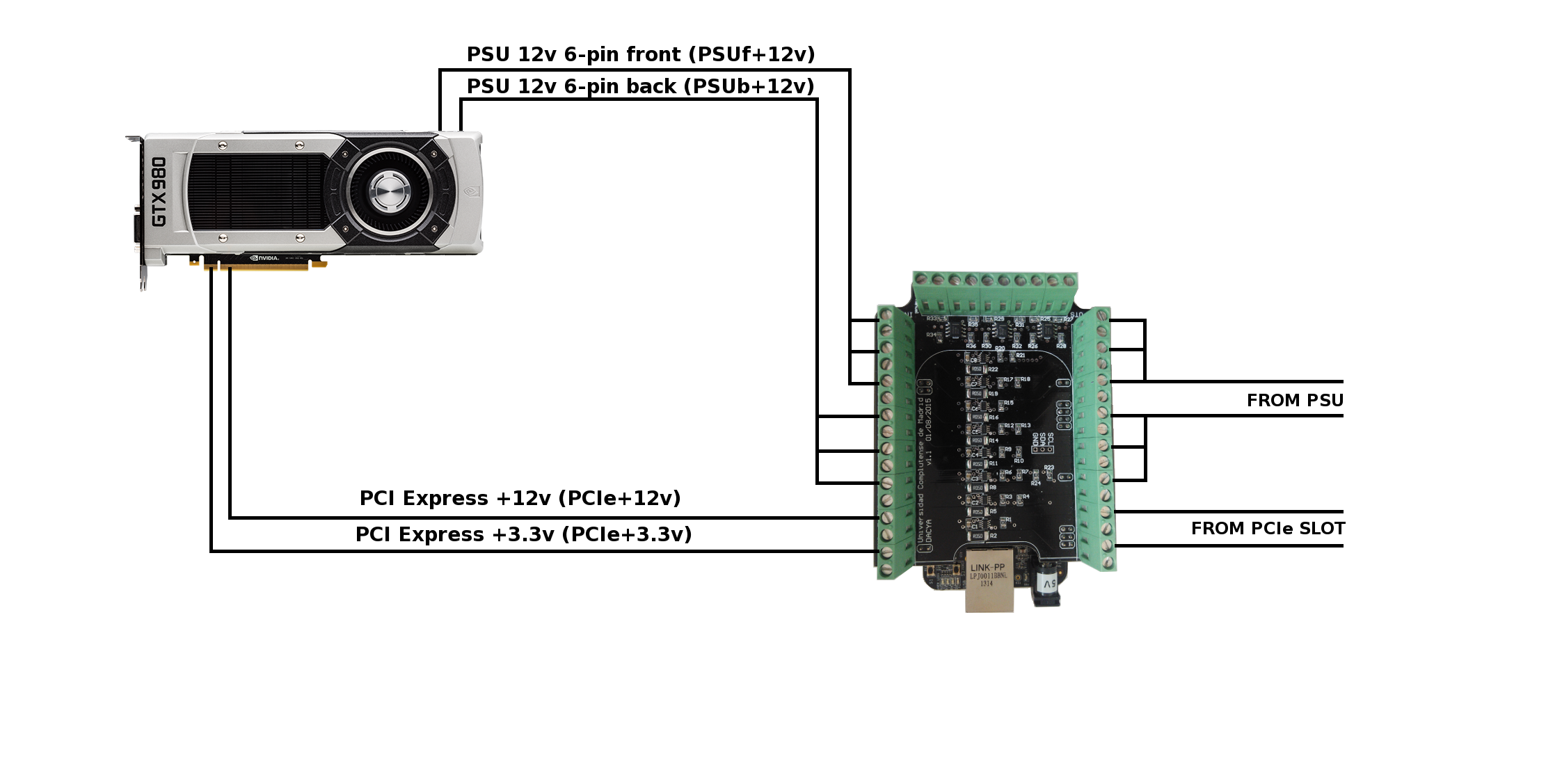
Figure 2: Wires, slots, cables and connectors for measuring energy on GPUs.

6.2 Software tool

Accelpower uses a modified version of pmlib library [54], a software package specifically created for monitoring energy. It consists of a server daemon that collects power data from devices and sends them to the clients, together with a client library for communication and synchronization with the server.

6.3 Methodology for Measuring Energy

The methodology for measuring energy begins with a start-up of the server daemon. Then, the source code of the application where the energy wants to be measured has to be modified to (1) declare pmlib variables, (2) clear and set the wires which are connected to the server, (3) create a counter and (4) start it. Once the code is over, we (5) stop the counter, (6) get the data, (7) save them to a .csv file, and (8) finalize the counter. See Figure 3 for a flow chart. Note that we get the instant consumption per measurement. Therefore, to obtain the global consumption, we compute the discrete integral over time.

Figure 3: Flow diagram for measuring energy on a code excerpt when running on the GPU.

Note that the homemade system we have built to measure real energy consumption can only be attached to a single GPU. That way, for obtaining performance or accuracy numbers, a single run suffices in multi-GPU environments, but energy requires a different approach. We have to move our measurement infrastructure from Pascal GPU to Maxwell GPU and perform different runs to monitor power values in both architectures. The final values are obtained multiplying those previous values by the number of GPUs. In case of four GPUs, we compute the energy for Maxwell and Pascal and aggregate them.

6.4 Hardware Resources

Our experimental study was conducted on a multi-GPU computer endowed with an Intel Xeon E5-2620 server and four PCI 3.0 slots to hold up to two Nvidia Titan X Pascal and two Titan X Maxwell GPUs. Table 2 summarizes major features for those GPUs. Note that cores and memory frequencies are overclocked to the maximum allowed by each GPU. The CPU has eight cores running at 2100 MHz and 64 GB of main memory running at 2400 MHz in a four-channel architecture. For secondary storage, we enable a Samsung SSD 850 EVO with a sequential reading up to 540 MB/s and an access time of 0.03 ms. On the software side, Ubuntu 14.04.4 LTS 64 bits was installed as the operating system together with CUDA 8.0.

Table 2: The set of Nvidia GPUs used along our experimental study.

Commercial model	Titan X	Titan X
GPU generation and year	Maxwell 2015	Pascal 2016
Raw computational power:
Number of cores	3072	3584
Cores frequency	1392 MHz	1911 MHz
Peak processing	6.6 TFLOPS	11 TFLOPS
CUDA Compute Capability	5.2	6.1
Dynamic memory (DRAM):
Size and type	12 GB GDDR5X	12 GB GDDR5X
Frequency and width	3505 MHz @ 384 bits	5005 MHz @ 384 bits
Bandwidth	336.5 GB/s	480 GB/s.
Static memory (cache):
Shared memory per multiprocessor	48 Kbytes	48 Kbytes
L2 cache	3 Mbytes	3 Mbytes
Thermal and energy specifications:
Maximum GPU Temperature	91 C	94 C
Peak Power Consumption (TDP)	250 W	250 W
Recommended supply Power	600 W	600 W

7 Input datasets

We cover a quantitative and qualitative analysis for a multi-GPU system, where each GPU executes evenly a subset or partition of the computation according to the workload distribution. Our experiments are conducted on a challenging dataset for gait recognition, TUM-GAID [55], and a huge dataset for image recognition, ILSVRC12 [11].

7.1 TUM-GAID

TUM-GAID (TUM Gait from Audio, Image and Depth) collects 305 subjects performing two walking trajectories in an indoor environment. The first trajectory is traversed from left to right and the second one from right to left. Two recording sessions were performed, one in January, where subjects wore heavy jackets and mostly winter boots, and another one in April, where subjects wore lighter clothes. The action is captured by a Microsoft Kinect sensor which provides a video stream with a resolution of $640\times 480$ pixels and a frame rate around 30 FPS. Figure  4 provides some examples.

Hereinafter the following nomenclature is used to refer each of the four walking conditions considered: normal walk (N), carrying a backpack of approximately 5 kg (B), wearing coating shoes (S, as used in clean rooms for hygiene conditions), and elapsed time (TN-TB-TS). During our experiments, we follow the experimental protocol defined by the authors of the dataset [55].

7.2 ILSVRC12

ImageNet Large-Scale Visual Recognition Challenge 2012 (ILSVRC12) is an annual competition which uses a subset of ImageNet. This subset is composed of 1000 classes with more than 1000 images per class. In total, there are roughly 1.2 million training images, 50,000 validation images, and 150,000 testing images. Those images have a variable resolution and have been manually annotated.

At test time, it is customary to report two accuracy rates: top-1 and top-5, where top-1 value is the classic accuracy metric and the top-5 accuracy rate is the fraction of test images for which the correct label is among the five most frequent labels considered by the model.

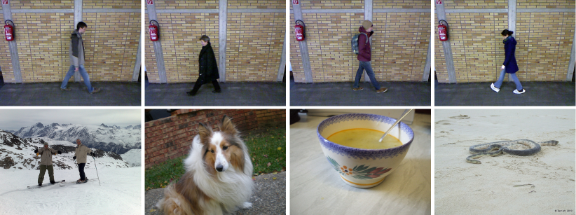
Figure 4: Our input datasets. Upper: TUM-GAID images from different subjects. Lower: ILSVRC1 images from different classes.

7.3 Customizing videos and images

For the experiments with ResNet and 2D-CNN, we resize all videos to a common resolution of $80\times 60$ pixels, keeping the original aspect ratio of video frames. This size exhibits a good trade-off between computational cost and recognition performance, as already reflected in a previous work  [46].

Given the resized video sequences, we compute dense OF on pairs of frames by using the method of Farneback [56] implemented in OpenCV library [57]. For each video frame, two OF frames are generated containing the $x$ and $y$ components of the flow vector. In parallel, people are located in a rough manner along the video sequences by background subtraction [58]. Then, we crop the video frames to remove part of the background and to align the subsequences (people are $x$-located in the middle of the central frame, #13), obtaining video frames of $60\times 60$ pixels (keeping the whole height).

Finally, from the cropped OF maps, we build subsequences of $25$ frames by stacking OF maps with an overlap of $\mathcal{O}\%$ frames. In our case, we choose $\mathcal{O}=80\%$, that is, to build a new subsequence, we use $20$ frames of the previous subsequence and $5$ new frames. For most state-of-the-start datasets, 25 frames cover almost one complete gait cycle [59]. Consequently, each OF volume has a size of $60\times 60\times 50$, which constitutes a sample for 2D-CNN and ResNet.

To increase the amount of training samples, we add mirror sequences and apply spatial displacements of $\pm 5$ pixels on each axis, obtaining a total of 8 new samples from each original sample.

For the experiments with CaffeNet, we resize all the images to a common resolution of $256\times 256$ pixels and, like in previous works [10], we do not keep the aspect ratio. During training, we perform random cropping and mirroring to obtain samples of $227\times 227$. In this case, we do not perform spatial displacements, but center cropping at test time.

During ResNet and 2D-CNN training, the weights are learnt using mini-batch stochastic gradient descent algorithm with momentum equal to $0.9$. We set weight decay to $5\cdot 10^{-4}$ and dropout to $0.4$ (when required). The number of epochs is limited to 20 and the learning rate is initially set to $10^{-2}$, to be decreased a $20\%$ every epoch.

During CaffeNet training, the weights are also learnt using mini-batch stochastic gradient descent algorithm with momentum equal to $0.9$. We set weight decay to $5\cdot 10^{-4}$ and dropout to $0.5$. The number of epochs is limited to 90 and the learning rate is initially set to $10^{-2}$, to be divided by $10$ every 20 epochs.

8 Experimental Results

Our testbed was executed on a multi-GPU server endowed with two Titan X Pascal and two Titan X Maxwell GPUs. The infrastructure for measuring time and energy was migrated from a Pascal GPU to a Maxwell one to gather all results shown along this section. For the sake of reliability and variance, we run all our experiments three times, and take the average as valid number. By using the same seed for the three experiments, the training process matches in all cases. Moreover, our tables distinguish rows in white for those CNNs using the TUM-GAID dataset (ResNet and 2D-CNN), and rows shaded for those CNNs using the ILSVRC12 dataset (CaffeNet and ResNetIm).

Table 3 shows the number of iterations and epochs executed for each CNN. Note that the number of epochs is the same along batch sizes but the number of iterations (i.e. batches) changes with the batch size. That way, the larger the batch size, the more samples are executed per iteration and less iterations are required to process training data.

Before we start discussing the experiments, let us introduce the section contents. In Sections 8.1 and 8.2, execution time and energy consumption are measured and discussed for forward and backward steps at batch level on Pascal and Maxwell GPUs. Also, different metrics are employed to compare and choose the best experimental setup for each device. In Section 8.3, a comparison between GPU generations is performed in terms of execution time and energy consumption. Section 8.4 performs a similar comparison for energy versus performance. Section 8.5 evaluates accuracy for the different trained models because a good model from either an energy or performance viewpoint is useless without a decent accuracy. Finally, Section 8.6 provides a guideline to select the best settings according to our findings.

Table 3: Iterations and epochs run for each CNN model and batch size.

	Batch size: 64		Batch size: 128		Batch size: 256
CNN model	Iterations	Epochs	Iterations	Epochs	Iterations	Epochs
ResNet	72 368	20	36 184	20	18 092	20
2D-CNN	72 368	20	36 184	20	18 092	20
CaffeNet	1 800 000	90	900 000	90	450 000	90
ResNetIm	1 800 000	90	900 000	90	450 000	90

8.1 Results on Pascal

Table 4: Execution times (in seconds) on a Pascal GPU for forward and backward steps of four CNN models using one, two and four GPUs and three batch sizes: 64, 128 and 256.

Forward
		Seconds per batch			Samples per second			Seconds for whole training
Batch size $\longrightarrow$		64	128	256	64	128	256	64	128	256
	ResNet	0.029	0.041	0.067	2 207	3 122	3 821	2 099	1 484	1 212
1 GPU	2D-CNN	0.013	0.029	0.057	4 923	4 414	4 491	941	1 049	1 031
	CaffeNet	0.013	0.027	0.053	4 923	4 741	4 830	23 400	24 300	23 850
	ResNetIm	0.075	0.144	-	853	889	-	135 000	129 600	-
	ResNet	0.025	0.030	0.041	2 560	4 267	6 244	1 809	1 086	742
2 GPUs	2D-CNN	0.008	0.014	0.027	8 000	9 143	9 481	579	507	488
	CaffeNet	0.008	0.014	0.027	8 000	9 143	9 481	14 400	12 600	12 150
	ResNetIm	0.040	0.074	0.138	1 600	1 730	1 855	72 000	66 600	62 100
	ResNet	0.029	0.032	0.040	2 207	4 000	6 400	2 099	1 158	724
4 GPUs	2D-CNN	0.007	0.012	0.023	9 143	10 667	11 130	507	434	416
	CaffeNet	0.007	0.014	0.024	9 143	9 143	10 667	12 600	12 600	10 800
	ResNetIm	0.035	0.062	0.112	1 829	2 065	2286	63 000	55 800	50 400
Backward
		Seconds per batch			Samples per second			Seconds for whole training
Batch size $\longrightarrow$		64	128	256	64	128	256	64	128	256
	ResNet	0.125	0.220	0.254	512	582	1 008	9 046	7 960	4 595
1 GPU	2D-CNN	0.021	0.048	0.094	3 048	2 667	2 723	1 520	1 737	1 701
	CaffeNet	0.026	0.053	0.105	2 462	2 415	2 438	46 800	47 700	47 250
	ResNetIm	0.188	0.369	-	340	347	-	338 400	332 100	-
	ResNet	0.069	0.115	0.205	928	1 113	1 249	4 993	4 161	3 709
2 GPUs	2D-CNN	0.018	0.029	0.051	3 556	4 414	5 020	1 303	1 049	923
	CaffeNet	0.037	0.045	0.071	1 730	2 844	3 606	66 600	40 500	31 950
	ResNetIm	0.099	0.181	0.337	646	707	760	178 200	162 900	151 650
	ResNet	0.053	0.105	0.184	1208	1 219	1 391	3 836	3 799	3 329
4 GPUs	2D-CNN	0.019	0.029	0.052	3 368	4 414	4 923	1 375	1 049	941
	CaffeNet	0.111	0.118	0.130	577	1 085	1 969	199 800	106 200	58 500
	ResNetIm	0.097	0.176	0.314	660	727	815	174 600	158 400	141 300

Table 5: Energy measurements (in joules) on a Pascal GPU for forward and backward steps of four CNN models using one, two and four GPUs and three batch sizes: 64, 128 and 256.

Forward
		Joules per batch			Joules per second			Joules for whole training
Batch size $\longrightarrow$		64	128	256	64	128	256	64	128	256
	ResNet	4.255	8.308	15.732	175	212	215	307 934	300 613	284 629
1 GPU	2D-CNN	3.891	8.335	16.614	225	240	248	281 552	301 580	300 576
	CaffeNet	3.203	6.552	12.428	227	223	243	5 764 522	5 896 956	5 592 634
	ResNetIm	17.331	31.707	-	229	213	-	31 195 884	28 535 892	-
	ResNet	2.721	4.274	8.529	151	169	211	196 931	154 633	154 305
2 GPUs	2D-CNN	1.754	4.126	8.951	219	250	268	126 948	149 305	161 949
	CaffeNet	1.818	3.307	6.782	204	210	222	3 272 331	2 976 198	3 052 121
	ResNetIm	8.441	17.280	30.902	212	229	214	15 194 106	15 552 276	13 905 941
	ResNet	2.222	2.797	4.322	136	143	173	160 833	101 200	78 185
4 GPUs	2D-CNN	0.776	1.819	3.372	247	222	232	56 177	65 833	61 012
	CaffeNet	0.813	1.901	3.323	228	214	209	1 464 046	1 711 015	1 495 398
	ResNetIm	4.692	9.054	16.837	214	225	222	8 446 127	8 148 414	7 576 728
Backward
		Joules per batch			Joules per second			Joules for whole training
Batch size $\longrightarrow$		64	128	256	64	128	256	64	128	256
	ResNet	15.990	28.531	26.714	194	185	177	1 157 146	1 032 357	483 313
1 GPU	2D-CNN	5.132	10.078	20.180	238	227	227	371 387	364 665	365 102
	CaffeNet	6.284	11.887	23.135	252	240	229	11 310 979	10 698 568	10 410 800
	ResNetIm	36.643	66.454	-	207	183	-	65 957 112	59 808 896	-
	ResNet	12.374	21.295	36.600	167	174	172	895 508	770 549	662 165
2 GPUs	2D-CNN	3.251	6.012	11.178	187	222	234	235 272	217 530	202 237
	CaffeNet	6.328	9.384	14.768	175	203	228	11 390 632	8 445 849	6 645 535
	ResNetIm	18.679	35.967	63.990	199	205	182	33 621 476	32 369 871	28 795 564
	ResNet	12.380	18.103	28.557	119	134	148	895 904	655 040	516 653
4 GPUs	2D-CNN	4.485	12.920	26.749	128	123	115	324 571	467 505	483 944
	CaffeNet	12.254	13.909	16.301	121	135	140	22 058 063	12 518 079	7 335 402
	ResNetIm	14.824	26.025	45.179	178	175	166	26 682 456	23 422 753	20 330 641

Table 6: Total execution time, energy consumption and EDP measurements for Pascal considering forward + backward steps of four CNN models using one, two and four GPUs and three batch sizes: 64, 128 and 256. Best results per measurement are boldfaced.

		Kiloseconds (ks)			Megajoules (MJ)			EDP
Batch size $\longrightarrow$		64	128	256	64	128	256	64	128	256
	1 GPU	11.1	9.4	5.8	1.47	1.33	0.77	16.3	12.6	4.5
ResNet	2 GPUs	6.8	5.2	4.5	2.18	1.85	1.63	14.9	9.7	7.3
	4 GPUs	5.9	5.0	4.1	4.30	3.05	2.28	25.5	15.1	9.2
	1 GPU	2.5	2.8	2.7	0.65	0.67	0.67	1.6	1.9	1.8
2D-CNN	2 GPUs	1.9	1.6	1.4	0.72	0.73	0.73	1.4	1.1	1.0
	4 GPUs	1.9	1.5	1.4	1.62	1.81	1.68	3.1	2.7	2.3
	1 GPU	70.2	72.0	71.1	17.08	16.60	16.00	1198.7	1194.9	1137.8
CaffeNet	2 GPUs	81.0	53.1	44.1	29.33	22.84	19.40	2375.4	1213.0	855.3
	4 GPUs	212.4	118.8	69.3	101.26	60.97	38.39	21508.0	7243.5	2660.6
	1 GPU	473.4	461.7	-	97.15	88.34	-	45992.2	40788.8	-
ResNetIm	2 GPUs	250.2	229.5	213.8	97.63	95.84	85.40	24427.3	21996.3	18254.9
	4 GPUs	237.6	214.2	191.7	146.39	132.87	120.61	34781.5	28460.5	23121.2

In this section we conduct experiments enabling the following hardware configurations: (1) one Pascal GPU , (2) two Pascal GPUs and (3) 2 Pascal + 2 Maxwell GPUs, with the measurement infrastructure always plugged to a Pascal GPU.

Table 4 shows execution times with three batch sizes: 64, 128 and 256. For ResNetIm, the batch of 256 samples was not executed because it does not fit within the GPU memory. The whole training process corresponds to the number of epochs shown in Table 3.

8.1.1 Forward step

According to the timing values (seconds per batch) shown in Table 4 for the forward step on a single GPU, the performance of 2D-CNN, CaffeNet and ResNetIm is very similar for different batch sizes. Best values for these networks are obtained for batch sizes of 64 (2D-CNN and CaffeNet) and 128 (ResNetIm). You realize much better when observing peak numbers in the column of samples processed per second. Also for one GPU, ResNet obtains larger performance gaps for different batch sizes, with poor results on small batches to reflect its dependency of aithmetic intensity. For the scalability of our implementations, using two GPUs 2D-CNN and Caffenet reach outstanding speedups (around 2.0x) on large batch sizes. Similar scores are attained by ResNetIm for any batch size, with its worst 1.6x speedup for the largest batch size. When moving to four GPUs, marginal improvements are seen, ranging from 2% (ResNet for a 256 batch size) to 19% (ResNetIm for 128 batch size). This is because the time is determined by the slowest GPU on Maxwell devices.

Last columns in Table 4 include the time required to compute all the forward iterations (shown in Table 3) to perform a complete training. On a single GPU, smaller values are obtained for large batch sizes in ResNet and RestNetIm. However, a batch size of 64 is better for 2D-CNN and CaffeNet. Extending to twin GPUs, time is significantly reduced in all cases, and again, we find marginal gains on four GPUs, even with scenarios where execution times slowdown a bit.

Table 5 shows in three main columns the joules per batch, joules per second (watts) and joules for whole training spent in the forward and backward step for three batch sizes. Note that power consumption is measured in one GPU. That way, when running the experiments on multiple GPUs, the energy spent must be multiplied by the number of GPUs to take into account all devices (that is on four GPUs, the total energy is the sum of two Pascals and two Maxwells). Starting on a single GPU, joules per batch increase as the batch size grows because more samples per batch are processed. Likewise, the value of joules per second is higher in most cases for larger batch sizes as more computational density is available. Joules spent for the whole training not only depend on the joules per second value (watts), but also on the number of samples processed per second (that is, the execution time for the whole training process). When considering all these aspects for the forward step, ResNet, CaffeNet and ResNetIm networks give their best for the largest batch sizes, while 2D-CNN does it for a batch size of 128. On multi-GPUs, joules per second for a specific batch size is smaller when using more GPUs to reflect the distribution of samples per batch.

8.1.2 Backward step

The backward step takes longer than the forward step (see samples per second for each case). We identify a peculiar behaviour in ResNet for a batch size of $256$ on a single GPU, where seconds per batch are very similar to those of a batch size of $128$ (in principle, it should double those times). Using the Nvidia CUDA Profiler for a closer analysis, we found that the last 5 convolutions using a batch size of $128$ are executed with the function wgrad_alg0_engine, whereas for the batch size of $256$, those convolutions call the function wgrad_alg1_engine. Those functions are automatically included in the final code by cuDNN. Comparing their execution times, wgrad_alg1_engine is quite faster than wgrad_alg0_engine to benefit the batch size of $256$. Using two GPUs, speedups are a bit lower than in the forward step, with the best value, 1.9x, to be reached for ResNet, 2D-CNN and ResNetIm for batch sizes of 128, 256 and 128, respectively. That indicates a good overlapping between kernels computation and AllReduce transfers. In CaffeNet, which has the lowest CDC, the kernel computation cannot hide completely the data transfer performed by AllReduce and, consequently, the multi-GPU version for this network reduces its speed-up to 1.5x for a batch size of 256, and even worse, when using four GPUs. The only network that obtains a significant improvement using four devices is ResNet with up to a 30% gain over the twin GPUs scenario.

Last columns in Table 4 show the time spent to compute all backward iterations (as shown in Table3) to perform a complete training. As already indicated in the forward step, on a single GPU, the process accelerates on lower batch sizes for ResNet and ResNetIm models. However, a batch size of 64 is better for 2D-CNN and CaffeNet. The use of two GPUs reduces the execution time in all forward and backward scenarios, but using four GPUs, only ResNet and ResNetIm improve during backward.

Table 5 shows the energy consumption for the backward step. On a single GPU, ResNet and ResNetIm networks consume less energy on larger batch sizes, whereas 2D-CNN and CaffeNet do it for a batch size of 64. For the multi-GPU case, joules per second for a specific batch size decrease when more GPUs are used, as the number of samples per batch is reduced and, consequently, less computation is performed.

8.1.3 Setup comparison

Now we compare all setups run on Pascal (i.e. number of GPUs, batch size and CNN models) to extract some conclusions regarding execution time, energy consumption and a combined metric of them, the Energy Delay Product (EDP) [60]. Table 6 summarizes those numbers for forward + backward steps during the complete training process. For a more compact representation, we measure time in kiloseconds (ks) and energy in Megajoules (MJ).

Focusing on execution time, the best option is a batch size of 256 samples for any network model. Depending on the type of architecture, it is better to use two GPUs for AlexNet-based models (2D-CNN and CaffeNet) and four GPUs for ResNet-based models (ResNet and ResNetIm).

For the energy exam, the best option is a batch size of 256 samples in most cases. Only with 2D-CNN it is better to use a small batch size of 64 samples, and only with ResNetIm we improve energy using two GPUs.

Finally, using the EDP metric, the best option overall is a large batch size with two GPUs. ResNet is an exception with one GPU as winner numbers due to the wgrad_alg1_engine problem already described in Section 8.1.2.

8.2 Results on Maxwell

Table 7: Execution times (in seconds) on a Maxwell GPU for forward and backward steps of four CNN models using one, two and four GPUs and three batch sizes: 64, 128 and 256.

Forward
		Seconds per batch			Samples per second			Seconds for whole training
Batch size $\longrightarrow$		64	128	256	64	128	256	64	128	256
	ResNet	0.039	0.059	0.094	1 641	2 169	2 723	2 822	2 135	1 701
1 GPU	2D-CNN	0.026	0.049	0.097	2 462	2 612	2 639	1 882	1 773	1 755
	CaffeNet	0.023	0.045	0.090	2 783	2 844	2 844	41 400	40 500	40 500
	ResNetIm	0.110	0.211	-	582	607	-	198 000	189 900	-
	ResNet	0.031	0.039	0.059	2 065	3 282	4 339	2 243	1 411	1 067
2 GPUs	2D-CNN	0.014	0.025	0.048	4 571	5 120	5 333	1 013	905	868
	CaffeNet	0.014	0.024	0.046	4 571	5 333	5 565	25 200	21 600	20 700
	ResNetIm	0.059	0.107	0.209	1 085	1 196	1 225	106 200	96 300	94 050
	ResNet	0.029	0.032	0.040	2 207	4 000	6 400	2099	1 158	724
4 GPUs	2D-CNN	0.007	0.012	0.023	9 143	10 667	11 130	507	434	416
	CaffeNet	0.007	0.014	0.024	9 143	9 143	10 667	12 600	12 600	10 800
	ResNetIm	0.035	0.062	0.112	1 829	2 065	2 286	63 000	5 5800	50 400
Backward
		Seconds per batch			Samples per second			Seconds for whole training
Batch size $\longrightarrow$		64	128	256	64	128	256	64	128	256
	ResNet	0.110	0.184	0.336	582	696	762	7 960	6 658	6 079
1 GPU	2D-CNN	0.039	0.074	0.148	1 641	1 730	1 730	2 822	2 678	2 678
	CaffeNet	0.047	0.092	0.182	1 362	1 391	1 407	84 600	82 800	81 900
	ResNetIm	0.269	0.520	-	238	246	-	484 200	468 000	-
	ResNet	0.049	0.078	0.135	1 306	1 641	1 896	3 546	2 822	2 442
2 GPUs	2D-CNN	0.025	0.045	0.080	2 560	2 844	3 200	1 809	1 628	1 447
	CaffeNet	0.044	0.060	0.103	1 455	2 133	2 485	79 200	54 000	46 350
	ResNetIm	0.141	0.261	0.512	454	490	500	253 800	234 900	230 400
	ResNet	0.053	0.105	0.184	1 208	1 219	1 391	3 836	3 799	3 329
4 GPUs	2D-CNN	0.019	0.029	0.052	3 368	4 414	4 923	1 375	1 049	941
	CaffeNet	0.111	0.118	0.130	577	1 085	1 969	199 800	106 200	58 500
	ResNetIm	0.097	0.176	0.314	660	727	815	174 600	158 400	141 300

Table 8: Energy measurements (in joules) on a Maxwell GPU for forward and backward steps of four CNN models using one, two and four GPUs and three batch sizes: 64, 128 and 256.

Forward
		Joules per batch			Joules per second			Joules for whole training
Batch size $\longrightarrow$		64	128	256	64	128	256	64	128	256
	ResNet	6.111	11.070	19.342	163	174	176	442 221	400 540	349 944
1 GPU	2D-CNN	6.248	12.199	24.432	208	208	214	452 148	441 402	442 022
	CaffeNet	5.379	10.499	21.217	209	206	215	9 681 859	9 448 940	9 547 708
	ResNetIm	22.864	45.341	-	201	203	-	41 155 296	40 807 243	-
	ResNet	3.988	6.188	11.183	154	156	172	288 620	223 899	202 325
2 GPUs	2D-CNN	3.052	6.272	12.221	194	213	217	220 855	226 959	221 108
	CaffeNet	2.995	5.255	10.615	185	196	203	5 391 093	4 729 650	4 776 933
	ResNetIm	12.581	22.611	45.459	226	199	206	22 646 534	20 349 928	20 456 374
	ResNet	2.979	4.075	6.350	141	152	156	215 574	147 466	114 892
4 GPUs	2D-CNN	1.530	3.146	6.003	192	207	219	110 705	113 847	108 603
	CaffeNet	1.493	3.103	5.381	193	206	204	2 686 577	2 792 498	2 421 440
	ResNetIm	6.043	11.620	21.899	190	188	192	10 876 855	10 457 805	9 854 684
Backward
		Joules per batch			Joules per second			Joules for whole training
Batch size $\longrightarrow$		64	128	256	64	128	256	64	128	256
	ResNet	13.012	23.047	45.465	166	172	178	941 655	833 920	822 555
1 GPU	2D-CNN	8.245	16.542	33.743	210	214	223	596 691	598 569	610 472
	CaffeNet	9.995	20.007	40.783	217	210	218	17 990 236	18 006 323	18 352 400
	ResNetIm	51.547	101.679	-	191	190	-	92 783 786	91 511 546	-
	ResNet	8.616	14.233	24.921	156	157	165	623 520	515 010	450 874
2 GPUs	2D-CNN	4.634	8.714	17.224	180	202	214	335 346	315 321	311 623
	CaffeNet	6.935	11.803	21.529	170	187	208	12 483 290	10 622 845	9 688 155
	ResNetIm	29.857	50.594	100.843	208	189	195	53 742 006	45 534 792	45 379 223
	ResNet	12.123	17.221	23.668	123	124	127	877 320	623 140	428 193
4 GPUs	2D-CNN	4.424	7.095	10.440	137	148	180	320 158	256 728	188 872
	CaffeNet	13.568	14.960	17.653	134	142	154	24 422 178	13 464 314	7 943 784
	ResNetIm	15.104	27.117	50.097	177	179	182	27 187 992	24 405 527	22 543 695

Table 9: Execution time, energy consumption and EDP measurements for Maxwell architecture considering forward + backward steps of four CNN models using one, two and four GPUs and three batch sizes: 64, 128 and 256. Best results per measurement are marked in bold.

		Kiloseconds (ks)			Megajoules (MJ)			EDP
Batch size $\longrightarrow$		64	128	256	64	128	256	64	128	256
	1 GPU	10.8	8.8	7.8	1.38	1.23	1.17	14.9	10.9	9.1
ResNet	2 GPUs	5.8	4.2	3.5	1.82	1.48	1.31	10.6	6.3	4.6
	4 GPUs	5.9	5.0	4.1	4.30	3.05	2.28	25.5	15.1	9.2
	1 GPU	4.7	4.5	4.4	1.05	1.04	1.05	4.9	4.6	4.7
2D-CNN	2 GPUs	2.8	2.5	2.3	1.11	1.08	1.07	3.1	2.7	2.5
	4 GPUs	1.9	1.5	1.4	1.62	1.81	1.68	3.1	2.7	2.3
	1 GPU	126.0	123.3	122.4	27.67	27.46	27.90	3486.7	3385.2	3415.0
CaffeNet	2 GPUs	104.4	75.6	67.1	35.75	30.70	28.93	3732.2	2321.3	1939.8
	4 GPUs	212.4	118.8	69.3	101.26	60.97	38.39	21508.0	7243.5	2660.6
	1 GPU	682.2	657.9	-	133.94	132.32	-	91373.2	87052.5	-
ResNetIm	2 GPUs	360.0	331.2	324.5	152.78	131.77	131.67	54999.7	43642.0	42720.7
	4 GPUs	237.6	214.2	191.7	146.39	132.87	120.61	34781.5	28460.5	23121.2

In this section, experiments are conducted using the following hardware configurations: (1) one Maxwell GPU, (2) two Maxwell GPUs and (3) 2 Pascal + 2 Maxwell GPUs, with the measurement infrastructure always plugged to a Maxwell GPU.

Table 7 shows execution times for three batch sizes: 64, 128 and 256. Again, the batch of 256 samples has not been executed for ResNetIm because it exceeds the GPU global memory size.

8.2.1 Forward step

Execution times follow a similar pattern to that already analyzed for Pascal, but as expected there is a general slowdown in performance because Maxwell is an older device. In the forward step, 2D-CNN, CaffeNet and ResNetIm all exhibit a stable throughput (samples per second) for any batch size, whereas ResNet reaches its peak for a batch size of 256. For two GPUs, excellent speedups values close to the optimal 2x are obtained for 2D-CNN, CaffeNet and ResNetImIn. A lower gain is achieved by ResNet. The configuration with four GPUs also produces excellent results with speeds around 4x for 2D-CNN and CaffeNet.

Table 8 shows power results measured following the same methodology described for Pascal. Again, the energy budget correlates with the execution time, but now power savings are smaller, basically because Maxwell was manufactured on 28 nm. transistors (Pascal benefits from a 16 nm. technology). For the forward step, lower energy requirements are typically achieved for larger batch sizes.

8.2.2 Backward step

Here, values on a single GPU follow tendencies already shown for the forward case. Twin GPUs exhibit good performance numbers for specific batch sizes, specially with ResNet and ResNetIm, to indicate effective overlapping between kernels computation and Allreduce transfers. Speedup values on four GPUs are modest, with improvements just for 2D-CNN and ResNetIm, and for the energy consumption, optimal values are found on larger batch sizes.

Table 8 shows power results measured following the same methodology described for Pascal. During the backward step, the benefit of using multiple GPUs during training is more clear compared to Pascal. Finally, comparing the whole process, forward plus backward, energy requirements are optimized on larger batches for all networks, what correlates with performance.

8.2.3 Setup comparison

As for Pascal, we compare here all setups run in Maxwell to draw some conclusions. Table 9 compiles all required numbers.

Starting with the execution time, again the best option is a batch size of 256 samples. Depending on the type of architecture, it is better to use two GPUs with network models having lower CTC (i.e. ResNet and CaffeNet) and 4 GPUs for the networks with higher CTC (i.e. 2D-CNN and ResNetIm).

For the energy discussion, the best option is a batch size of 256 samples with ResNet-based models (ResNet/ResNetIm) and 128 samples with AlexNet-based models (2D-CNN/CaffeNet). And best records are registered on a single GPU, with the exception of ResNetIm on 4 GPUs.

Finally, for the EDP metric, the best option is a large batch size with two GPUs for networks with low CTC. For higher CTC values, optimal values are found on larger batch size using four GPUs.

8.3 Pascal versus Maxwell

We now want to compare the execution time and power consumption of our four CNN models for all batch sizes and number of GPUs on Maxwell and Pascal. These results are compiled in Figures 5, 6, 7 and 8. For the bar names in our charts, we follow the rule batch_size-number_GPUs. For example, 64-4 stands for a batch of 64 elements using 4 GPUs. Again, there are fluctuations in 4 GPUs because the two Pascals have to wait the two Maxwells to conclude. This effect can only be seen in energy consumption because the time included in the plots is the slowest of all GPUs (that is, time measurements for Maxwell match those of Pascal when using 4 GPUs).

Results indicate that for 2D-CNN, CaffeNet and ResNetIm, Pascal is ahead in performance and power consumption. The improvement can be quantified within a $30-40\%$ range depending on the experiment. For ResNet, performance drops in Pascal versus Maxwell when using multiple GPUs, and also on a single GPU for small batch sizes. To explain this behaviour, we have added Table 10 specifically for ResNet, covering all batch sizes and GPUs. As we can see, during forward, the behaviour is around $30\%$ better in Pascal. However, during backward, its performance decreases heavily and Maxwell overtakes it. We have found Pascal to be affected by the algorithm change used within cuDNN to compute the last convolutions of this model (wgrad_alg0_engine method instead of wgrad_alg1_engine, being the former 25 times slower than the latter - see Section 8.1). The only value which is not affected by this anomaly in Table 10 is the batch size of $256$ executed in one GPU (when using more GPUs, the batch size is distributed among them, and the threshold for the algorithm to switch to the swift version is never reached). This way, results worsen when using Pascal with ResNet if the threshold in the batch size is not reached, regardless of the number of GPUs. We are confident this anomaly will be solved in future releases of cuDNN to end up with faster executions like all those we have introduced here using the wgrad_alg1_engine method.

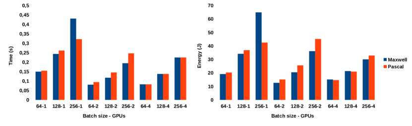
Figure 5: Comparative between Maxwell and Pascal for ResNet. (left) time per batch (right) joules per batch. All measurements are for forward + backward steps using 1, 2 and 4 GPUs and three batch sizes: 64, 128 and 256.

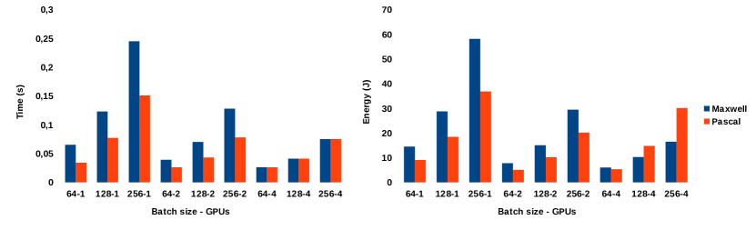
Figure 6: Comparative between Maxwell and Pascal for 2D-CNN. Left: time per batch. Right: joules per batch. All measurements are for forward + backward steps using 1, 2 and 4 GPUs and three batch sizes: 64, 128 and 256.

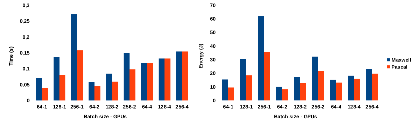
Figure 7: Comparative between Maxwell and Pascal for CaffeNet. Left: time per batch. Right: joules per batch. All measurements are for forward + backward steps using 1, 2 and 4 GPUs and three batch sizes: 64, 128 and 256.

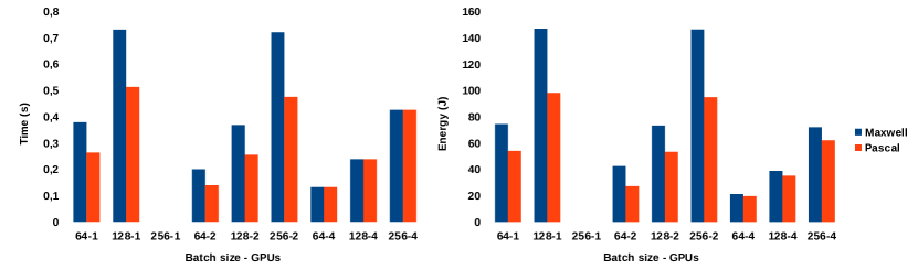
Figure 8: Comparative between Maxwell and Pascal for ResNetIm. Left: time per batch. Right: joules per batch. All measurements are for forward + backward steps using 1, 2 and 4 GPUs and three batch sizes: 64, 128 and 256.

Table 10: A comparison between Maxwell and Pascal during forward and backward steps using ResNet.

Forward
		Time per batch			Joules per batch
	Batch size	Maxwell	Pascal	$\%$	Maxwell	Pascal	$\%$
	64	0.039	0.029	25.6	6.111	4.255	30.4
1 GPU	128	0.059	0.041	30.5	11.070	8.308	24.9
	256	0.094	0.067	28.7	19.342	15.732	18.7
	64	0.031	0.025	19.4	3.988	2.721	31.8
2 GPUs	128	0.039	0.030	23.1	6.188	4.274	30.9
	256	0.059	0.041	30.5	11.183	8.529	23.7
	64	0.029	0.029	0	2.979	2.222	25.4
4 GPUs	128	0.032	0.032	0	4.075	2.797	31.4
	256	0.040	0.040	0	6.350	4.322	31.9
Backward
		Time per batch			Joules per batch
	Batch size	Maxwell	Pascal	$\%$	Maxwell	Pascal	$\%$
	64	0.110	0.125	-13.6	13.012	15.990	-22.9
1 GPU	128	0.184	0.220	-19.6	23.047	28.531	-23.8
	256	0.336	0.254	24.4	45.465	26.714	41.2
	64	0.049	0.069	-40.8	8.616	12.374	-43.6
2 GPUs	128	0.078	0.115	-47.4	14.233	21.295	-49.6
	256	0.135	0.205	-51.9	24.921	36.600	-46.9
	64	0.053	0.053	0	12.123	12.380	-2.1
4 GPUs	128	0.105	0.105	0	17.221	18.103	-5.1
	256	0.184	0.184	0	23.668	28.557	-20.7

8.4 Energy versus performance

In general, the GPU evolution has demonstrated that performance does not correlate ideally with energy efficiency, because sometimes you experience severe power penalties when being eager on performance. In fact, Nvidia introduced GPU Boost and clock monitoring in Kepler GPUs back in 2012 to keep an eye on power at run time depending on computational requirements driven by every particular application. Later in 2014, when they released Maxwell, it was announced as the most power efficient GPU ever built [61]. Compared to its predecessor Kepler, multiprocessors were reduced to 128 cores and layout was reorganized into quadrants to shorten wires length. Communications and power lines were identified primary factors in energy consumption, so it was no surprise to find Maxwell ahead a 2x factor in performance per watt.

Enhancements introduced in 2016 with Pascal were driven by performance and energy, but with certain tradeoffs versus Maxwell. Focusing on Titan models to be fair, Table 2 summarizes features for the two GPUs used in our study. The Maxwell model contains 3072 cores at 1392 MHz clock rate, whereas the Pascal counterpart has 3584 cores running at 1911 MHz. The number of transistors on a chip and its frequency affect power in a linear way, which leads us to estimate Pascal around 65% higher on energy demand, and presumably a similar percentage ahead in performance. When you increase wattage but reduce seconds proportionally, the energy toll in joules should remain constant, but there were good news for Pascal on a performance-per-watt basis: Multiprocessors were reduced to 64 cores and, overall, manufacturing process evolved from planar 28 nm. transistors to 16 nm. fin-FET ones [62]. With those many variables affecting power and all side-effects among them, it is complex to assess pros and cons to determine a winner of the energy battle, and even more challenging to put differences in raw numbers.

Our set of experiments may shed some light driven by praxis. Table 11 illustrates performance per watt on a wide number of settings, changing CNN models and batch sizes. Peak numbers are reached on one GPU computing the 2D-CNN model, where numbers are stable around 11 GFLOPS/w for Pascal and 7 GFLOPS/w for Maxwell (around 60% deficit). 2D-CNN is also the optimal model on two GPUs, keeping distances between twin Pascals and twin Maxwells around 50%. Official peak differences published by Nvidia in double precision numbers are 40% (20 GFLOPS/w for an average Pascal GPU and 12 GFLOPS/w for the Maxwell counterpart), what tells us that we have found CNN models where those differences widen up to an additional 20% regardless of the batch size chosen. We also see that energy efficiency is very sensitive to the CNN model computed, because there are other cases, like the ResNet model, where differences shorten very much among GPUs.

Our numbers also validate Nvidia estimations, because our global average for all models and batch sizes is 42% running on a single GPU and 35% when using a pair. The 4 GPUs setup may look confusing at first sight, but note that we are not comparing 4 Pascals versus 4 Maxwells. Instead, we always use 2 Pascals plus 2 Maxwells, that is, it is always the same run, just changing power measurements from one generation to another. That way, synchronizations may relax the faster twin Pascals to end up with similar power requirements versus the twins Maxwells. In other words, performance is mainly responsible for energy savings when running CNNs on Pascal, and the set of experiments gathered in this paper encourage you to press the throttle because you will not end up paying more on fuel.

In addition, we can see that CNN applications stay, in general, far from optimal performance per watt ratios: The maximum values we were able to attain are 11 GFLOPS/w on a Pascal and 7 GFLOPS/w on a Maxwell, whereas SGEMM (Single Precision General Matrix Multiply) reaches 42 GFLOPS/w in Pascal and 23 GFLOPS/w in Maxwell. That means that we barely squeeze 25% of the performance efficiency exhibited by a typical compute bound procedure. We expect this margin to shrink when using the new half data types that Nvidia introduced in Pascal particularly to benefit deep learning applications.

Finally, if we focus our analysis on the influence of the batch size, optimal performance and minimum energy consumption due to savings in training time are attained when increasing batch sizes as much as possible in all GPU scenarios. But there are a number of concerns regarding accuracy and datasets which deserve a closer attention. We address those two in sections 8.5 and 8.6, respectively.

Table 11: GFLOPS per watt for our four CNN models with three batch sizes measured on Pascal and Maxwell using 1, 2 and 4 GPUs (note that the 4 GPUs run is the same for Pascal and Maxwell, we just change the device where energy is measured). Results including both forward and backward. Averages are calculated per row and column, and last column reflects differences based on those.

GFLOPS/w measured on $\longrightarrow$		Pascal				Maxwell				Pascal
Batch size $\longrightarrow$		64	128	256	Average	64	128	256	Average	gain
	ResNet	2.7	3.0	5.1	4.3	2.8	3.2	3.4	3.1	38%
1 GPU	2D-CNN	11.1	10.9	10.9	11.0	6.9	7.0	6.9	6.9	59%
(1 Pascal or	CaffeNet	9.8	10.1	10.5	10.1	6.1	6.1	6.0	6.1	65%
1 Maxwell)	ResNetIm	4.9	5.4	-	5.1	3.6	3.6	-	3.6	41%
	Average	7.1	7.3	8.8	7.7	5.8	5.0	5.4	5.4	+42%
	ResNet	1.8	2.1	2.4	2.1	2.2	2.7	3.0	2.6	-20%
2 GPUs	2D-CNN	10.0	9.9	10.0	10.0	6.5	6.7	6.8	6.7	49%
(2 Pascals or	CaffeNet	5.7	7.3	8.6	7.2	4.7	5.5	5.8	5.3	35%
2 Maxwells)	ResNetIm	4.9	5.0	5.6	5.2	3.1	3.6	3.6	3.4	52%
	Average	5.6	6.1	6.6	6.1	4.1	4.6	4.8	4.5	+35%
	ResNet	0.9	1.3	1.7	1.3	0.9	1.3	1.8	1.3	0%
4 GPUs	2D-CNN	4.8	3.4	3.3	4.2	4.2	4.9	6.1	5.0	-16%
(2 Pascals and	CaffeNet	1.8	2.9	4.7	3.1	1.5	2.6	4.0	2.7	14%
2 Maxwells)	ResNetIm	3.4	3.8	4.3	3.8	3.1	3.4	3.7	3.4	11%
	Average	2.8	2.9	3.5	3.1	2.4	3.0	3.9	3.1	0%

8.5 Accuracy

We extend our CNN analysis from performance and energy viewpoints in this section to find a good model in terms of accuracy. In our experiments, we only consider the batch size as tunable hyper-parameter, because all remaining ones have been taken from previously trained models with good accuracy. According to Caffe’s implementation, the training with one or more GPUs leads to the same results, so we do not move the number of GPUs. Moreover, we distinguish results taken from models using videos as input (Table 12) from those using images (Table 13).

Table 12 summarizes the accuracy results for ResNet and 2D-CNN, where we can see that the best model is 2D-CNN with $86.0\%$ of accuracy. On the other hand, the best ResNet model obtains a disappointing $76\%$. Overfitting is responsible for this low accuracy. This model contains a vast number of parameters, while the amount of training data available in the dataset is relatively small. Therefore, the model is not able to generalize to the test data. Comparing the accuracy among batch sizes in both models, the precision decreases with bigger batches because the average gradients are less noisy and the exploration capacity of the algorithm is reduced. On the other hand, with small batches, the algorithm explores better the solution space and, consequently, finds a better local minimum. This effect is more clear in ResNet due to the huge amount of parameters. In 2D-CNN, accuracy is much less sensitive to the batch size, showing differences around $4\%$, so we may select any batch size or prioritize the choice based on performance and/or energy criteria.

Table 13 shows the accuracy values for ResNetIm and CaffeNet. We report top-1 and top-5 ac curacies, where the top-1 is the classic accuracy and the top-5 is the the percentage of test images for which the correct label is among the five most frequent labels considered by the model. On image datasets, the more training data are available, the more performance gap in favor of ResNet. Moreover, the large number of parameters allows to fit a more discriminant model, overtaking CaffeNet by more than a $10\%$ in Top-5 and almost $20\%$ in Top-1.

Along batch sizes, all models experience accuracy improvements on larger batches. Again, the vast amount of training data available in ImageNet requires larger batch sizes to compute more accurate gradients during the training process. On small batch sizes, the average gradient of the batch, which is used to update the parameters of the network, separates from the mean of the complete training set being more noisy, and therefore, worsening updates.

Table 12: Accuracy on TUM-GAID. We deploy different CNN models and batch sizes in rows, and scenarios (temporal and non temporal) in columns. The last column ‘AVG’ stands for the average of each case weighted by the number of classes. Best average results are boldfaced.

Model	Batch size	N	B	S	TN	TB	TS	AVG
ResNet	64	89.0	76.4	72.2	43.5	47.0	45.0	76.0
	128	71.9	62.6	62.3	33.8	37.4	36.3	62.8
	256	63.5	52.7	56.1	32.8	35.5	38.1	55.4
2D-CNN	64	95.7	87.5	87.1	45.6	47.2	47.4	86.0
	128	95.5	84.9	83.9	51.2	41.5	51.5	84.4
	256	95.3	79.2	81.2	48.6	39.5	51.7	81.6

Table 13: Accuracy on ImageNet. CNN models and batch sizes are drawn by rows, and metrics (top-1 and top-5 accuracy) by columns. Top-1 is the classic accuracy and the top-5 is the the percentage of test images for which the correct label is among the five labels considered most frequent by the model. Best average results are boldfaced.

Model	Batch size	Top-1	Top-5
CaffeNet	64	44.0	68.7
	128	52.9	76.7
	256	57.3	80.4
ResNetIm	64	61.6	84.7
	128	65.6	88.5
	256	75.3	92.2

8.6 Best approach

We now summarize the information obtained from our experiments to propose some guidelines to choose the best hyper-parameters according to performance, energy consumption and accuracy criteria.

The road to maximize performance and minimize training time and energy consumption leads to larger batch sizes as shown in Tables 6 and 9. On the contrary, when accuracy is a must, small batches should be used on regular datasets. Big datasets enable a wider range of batch sizes, and depending on the problem, chances to find a good combination of time, energy and accuracy increase. When multiple GPUs are available, setups with more than a pair of them must be carefully studied fas transfers and synchronizations can hurt performance, particularly on a set of heterogeneous GPUs.

In general, when small and challenging datasets are used, we have to choose between performance/energy or accuracy, but there are exceptions too. For example, 2D-CNN reaches good accuracy at any batch size. This may indicate that any CNN composed solely of 2D convolutions (without batch normalization and residual connections) can use large batches to save time and energy while retaining accuracy. On the other hand, ResNet networks rely on small batches for gaining accuracy at the expense of performance and power consumption. Fortunately, this scenario does not predominate and occurs just on challenging datasets like TUM-GAID.

On large datasets, state-of-the-art accuracy is obtained with a large batch size like 256 samples. In cases like ILSVRC, thanks to the noise effect in the gradients, we have it all: optimal accuracy, maximum performance and minimum energy requirements.

In summary, for large datasets the best option is always a large batch size regardless of the CNN used, and for small datasets, large batches are only useful with networks without batch normalization and residual connections. Should a ResNet be used, we use a small batch paying a toll in terms of performance and power consumption. And on a multi-GPU system, it would be convenient to fill all slots available with GPUs alike.

9 Summary and Conclusions

In this paper, we have presented a performance, energy and accuracy analysis on a set of popular CNN models running on flagship image and video applications for different training sets and parameters setting using the last two Nvidia GPU generations, namely Maxwell and Pascal (Titan versions). Our goal is to provide an empirical study using state-of-art CNNs with applied datasets and carefully selecting parameters of major interest for researchers to tune Deep Learning methods. They work on understanding how set-ups may help inferences, we evaluate how efficient they are, primarily from an energy viewpoint, but also considering speed-ups and numerical accuracy.

Major contributions of this work can be summarized as follows:

1. We were never able to squeeze more than 55% of the peak power efficiency announced by Nvidia: 20 and 12 GFLOPS/w using the worst-case scenario of 64-bit data types on Pascal and Maxwell, respectively.

2. The performance per watt gap between Maxwell and Pascal GPUs was found to reach peaks of up to 60%, with differences sensitive to the CNN model and batch size.

3. If we separate performance and energy, Pascal attains solid differences within the $30-40\%$ range depending on the batch size for 2D-CNN, CaffeNet and ResNetIm CNN models, in line with Nvidia estimations.

4. Forward and backward steps show similar behaviour in almost all scenarios, extending performance and power gains on larger CNN batches.

5. Accuracy prefers small batches on small datasets, but sometimes keeps stable on large batches for us to prioritize speed and energy without worsening results. On big datasets, larger batch sizes minimize trade offs among those three.

6. Datasets play an important role associated to every CNN model, sometimes being responsible of inconsistencies and thermal stress in GPU hardware when complexity increases.

7. In multi-GPU environments, the batch size plays an important role because the GPU code reduces its arithmetical intensity and becomes less compute-bound, thus requiring larger sizes to hide the communication and synchronization overhead. In particular, when using four or more GPUs, models trained are required to be huge for communications to effectively overlap computations. And heterogeneity in GPU hardware also introduces additional hurdles for these communication costs.

We envision GPUs to increase their role as high performance and low power devices for CNNs and Deep Learning applications in future GPU generations, particularly after the introduction of the 3D memory in 2017 and the Volta generation by Nvidia. Volta increases the number of cores from 3584 to 5120 to leverage speedups, and relaxes frequency from 1480 to 1455 MHz with transistors shrinking from 16 to 12 nm. for a more complete low-power device and ambitious GFLOPS/w ratio. Endowing Volta with half precision data types and Tensor cores will also affect performance, energy and accuracy in a very positive manner, leaving room for a promising scalability to constitute the next step of our analysis as future work.

References

- [1] Goodfellow I, Bengio Y, Courville A. Deep Learning. MIT Press, 2016. http://www.deeplearningbook.org.
- [2] Lowe DG. Object recognition from local scale-invariant features. Proceedings of the Seventh IEEE International Conference on Computer Vision, vol. 2, 1999; 1150–1157 vol.2.
- [3] Wang H, Kläser A, Schmid C, Liu CL. Action recognition by dense trajectories. CVPR 2011, 2011; 3169–3176, doi:10.1109/CVPR.2011.5995407.
- [4] Castro FM, Marín-Jiménez M, Guil Mata N, Muñoz Salinas R. Fisher motion descriptor for multiview gait recognition. International Journal of Patt. Recogn. in Artificial Intelligence 2017; 31(1).
- [5] Castro FM, Marín-Jiménez MJ, Guil N. Multimodal features fusion for gait, gender and shoes recognition. Machine Vision and Applications Nov 2016; 27(8):1213–1228.
- [6] Fukushima K. Neocognitron: A self-organizing neural network model for a mechanism of pattern recognition unaffected by shift in position. Biological Cybernetics Apr 1980; 36(4):193–202.
- [7] Lecun Y, Bottou L, Bengio Y, Haffner P. Gradient-based learning applied to document recognition. Proceedings of the IEEE Nov 1998; 86(11):2278–2324.
- [8] Serre T, Wolf L, Bileschi S, Riesenhuber M, Poggio T. Robust object recognition with cortex-like mechanisms. IEEE Transactions on Pattern Analysis and Machine Intelligence 2007; 29(3):411–426.
- [9] Cortes C, Vapnik V. Support-vector networks. Machine Learning Sep 1995; 20(3):273–297.
- [10] Krizhevsky A, Sutskever I, Hinton GE. Imagenet classification with deep convolutional neural networks. Advances in Neural Information Processing Systems, 2012; 1097–1105.
- [11] Russakovsky O, Deng J, Su H, Krause J, Satheesh S, Ma S, Huang Z, Karpathy A, Khosla A, Bernstein M, et al.. ImageNet Large Scale Visual Recognition Challenge. International Journal of Computer Vision (IJCV) 2015; 115(3):211–252, doi:10.1007/s11263-015-0816-y.
- [12] Krizhevsky A. Learning multiple layers of features from tiny images. Technical Report, University of Toronto 2009.
- [13] Abu-El-Haija S, Kothari N, Lee J, Natsev P, Toderici G, Varadarajan B, Vijayanarasimhan S. Youtube-8m: A large-scale video classification benchmark. ArXiv e-prints 2016; .
- [14] Szegedy C, Liu W, Jia Y, Sermanet P, Reed S, Anguelov D, Erhan D, Vanhoucke V, Rabinovich A. Going deeper with convolutions. 2015 IEEE Conference on Computer Vision and Pattern Recognition (CVPR), 2015; 1–9.
- [15] He K, Zhang X, Ren S, Sun J. Delving deep into rectifiers: Surpassing human-level performance on imagenet classification. 2015 IEEE International Conference on Computer Vision (ICCV), 2015; 1026–1034.
- [16] Simonyan K, Zisserman A. Two-stream convolutional networks for action recognition in videos. Advances in Neural Information Processing Systems, 2014; 568–576.
- [17] Wang L, Qiao Y, Tang X. Action recognition with trajectory-pooled deep-convolutional descriptors. 2015 IEEE Conference on Computer Vision and Pattern Recognition (CVPR), 2015; 4305–4314.
- [18] Ren S, He K, Girshick R, Sun J. Faster r-cnn: Towards real-time object detection with region proposal networks. Proceedings of the 28th International Conference on Neural Information Processing Systems - Volume 1, NIPS’15, 2015; 91–99.
- [19] Liu W, Anguelov D, Erhan D, Szegedy C, Reed S, Fu CY, Berg AC. SSD: Single Shot MultiBox Detector. Springer International Publishing: Cham, 2016; 21–37.
- [20] Marín-Jiménez MJ, Castro FM, Guil N, de la Torre F, Medina-Carnicer R. Deep multitask learning for gait-based biometrics. Proceedings of the IEEE International Conference on Image Processing, 2017.
- [21] Castro FM, Marín-Jiménez MJ, Guil N, López-Tapia S, de la Blanca NP. Evaluation of cnn architectures for gait recognition based on optical flow maps. BIOSIG, 2017; 251–258.
- [22] Jia Y, Shelhamer E, Donahue J, Karayev S, Long J, Girshick R, Guadarrama S, Darrell T. Caffe: Convolutional architecture for fast feature embedding. arXiv preprint arXiv:1408.5093 2014; .
- [23] Abadi M, Agarwal A, Barham P, Brevdo E, Chen Z, Citro C, Corrado GS, Davis A, Dean J, Devin M, et al.. TensorFlow: Large-scale machine learning on heterogeneous systems 2015. URL https://www.tensorflow.org/, software available from tensorflow.org.
- [24] Seide F, Agarwal A. Cntk: Microsoft’s open-source deep-learning toolkit. Proceedings of the 22Nd ACM SIGKDD International Conference on Knowledge Discovery and Data Mining, KDD ’16, 2016; 2135–2135.
- [25] Vedaldi A, Lenc K. MatConvNet – Convolutional Neural Networks for MATLAB. Proceeding of the ACM Int. Conf. on Multimedia, 2015.
- [26] Paszke A, Gross S, Chintala S, Chanan G, Yang E, DeVito Z, Lin Z, Desmaison A, Antiga L, Lerer A. Automatic differentiation in pytorch 2017; .
- [27] The Green 500 Supercomputers List. http://www.top500.org/green500.
- [28] Shi S, Wang Q, Xu P, Chu X. Benchmarking state-of-the-art deep learning software tools. 2016 7th International Conference on Cloud Computing and Big Data (CCBD), 2016; 99–104.
- [29] Kim H, Nam H, Jung W, Lee J. Performance analysis of cnn frameworks for gpus. 2017 IEEE International Symposium on Performance Analysis of Systems and Software (ISPASS), 2017; 55–64.
- [30] Dong S, Gong X, Sun Y, Baruah T, Kaeli D. Characterizing the microarchitectural implications of a convolutional neural network (cnn) execution on gpus. Proceedings of the 2018 ACM/SPEC International Conference on Performance Engineering, ICPE ’18, 2018; 96–106.
- [31] Benedict S. Energy-aware performance analysis methodologies for hpc architectures — an exploratory study. Journal of Network and Computer Applications 2012; 35(6):1709–1719.
- [32] Jouppi N. Google supercharges machine learning tasks with TPU custom chip. https://cloudplatform.googleblog.com/2016/05/Google-supercharges-machine-learning-tasks-with-custom-chip.html.
- [33] Moons B, Brabandere BD, Gool LV, Verhelst M. Energy-efficient convnets through approximate computing. 2016 IEEE Winter Conference on Applications of Computer Vision (WACV), 2016; 1–8, doi:10.1109/WACV.2016.7477614.
- [34] Cai E, Juan D, Stamoulis D, Marculescu D. Neuralpower: Predict and deploy energy-efficient convolutional neural networks. CoRR 2017; abs/1710.05420. URL http://arxiv.org/abs/1710.05420.
- [35] Andri R, Cavigelli L, Rossi D, Benini L. Yodann: An ultra-low power convolutional neural network accelerator based on binary weights. 2016 IEEE Computer Society Annual Symposium on VLSI (ISVLSI), 2016; 236–241, doi:10.1109/ISVLSI.2016.111.
- [36] Yang T, Chen Y, Sze V. Designing energy-efficient convolutional neural networks using energy-aware pruning. CoRR 2016; abs/1611.05128. URL http://arxiv.org/abs/1611.05128.
- [37] Deep Neural Network Energy Estimation Tool. https://energyestimation.mit.edu.
- [38] Lin Y, Sakr C, Kim Y, Shanbhag N. Predictivenet: An energy-efficient convolutional neural network via zero prediction. 2017 IEEE International Symposium on Circuits and Systems (ISCAS), 2017; 1–4, doi:10.1109/ISCAS.2017.8050797.
- [39] Mathew M, Desappan K, P KS, S N, Moothedath B. Embedded low-power deep learning with tidl. Texas Instruments Technical Report 2018; .
- [40] Bettoni M, Urgese G, Kobayashi Y, Macii E, Acquaviva A. A convolutional neural network fully implemented on fpga for embedded platforms. 2017 New Generation of CAS (NGCAS), 2017; 49–52, doi:10.1109/NGCAS.2017.16.
- [41] Wang Y, Xia L, Tang T, Li B, Yao S, Cheng M, Yang H. Low power convolutional neural networks on a chip. 2016 IEEE International Symposium on Circuits and Systems (ISCAS), 2016; 129–132, doi:10.1109/ISCAS.2016.7527187.
- [42] Mathew M, Desappan K, P KS, Nagori S, Moothedath B. Sparse, quantized, full frame cnn for low power embedded devices. Proceedings Computer Vision and Pattern Recognition (CVPR), 2017.
- [43] Farabet C, Couprie C, Najman L, LeCun Y. Learning hierarchical features for scene labeling. IEEE Transactions on Pattern Analysis and Machine Intelligence 2013; 35(8):1915–1929.
- [44] Zhang X, Zhao J, LeCun Y. Character-level convolutional networks for text classification. Advances in Neural Information Processing Systems, IEEE, 2015.
- [45] Wang Y, Long M, Wang J, Yu PS. Spatiotemporal pyramid network for video action recognition. The IEEE Conference on Computer Vision and Pattern Recognition (CVPR), 2017.
- [46] Castro FM, Marín-Jiménez MJ, Guil N, Pérez de la Blanca N. Automatic learning of gait signatures for people identification. Advances in Computational Intelligence: 14th International Work-Conference on Artificial Neural Networks (IWANN) 2017; :257–270.
- [47] He K, Zhang X, Ren S, Sun J. Deep residual learning for image recognition. Proceedings of the IEEE Conference on Computer Vision and Pattern Recognition (CVPR), 2016; 770–778.
- [48] Zhang C, Li P, Sun G, Guan Y, Xiao B, Cong J. Optimizing fpga-based accelerator design for deep convolutional neural networks. Proceedings of the 2015 ACM/SIGDA International Symposium on Field-Programmable Gate Arrays, FPGA ’15, 2015; 161–170.
- [49] Chetlur S, Woolley C, Vandermersch P, Cohen J, Tran J, Catanzaro B, Shelhamer E. cudnn: Efficient primitives for deep learning. CoRR 2014; abs/1410.0759.
- [50] BeagleBone. Beaglebone black. http://beagleboard.org/BLACK.
- [51] González-Rincón J. Sistema basado en open source hardware para la monitorización del consumo de un computador. Master Thesis Project. Universidad Complutense de Madrid 2015; .
- [52] Ada L. Adafruit INA219 Current Sensor Breakout. https://learn.adafruit.com/adafruit-ina219-current-sensor-breakout.
- [53] Igual F, Jara L, Gómez J, Piñuel L, Prieto M. A Power Measurement Environment for PCIe Accelerators. Computer Science - Research and Development May 2015; 30(2):115–124.
- [54] Alonso P, Badía R, Labarta J, Barreda M, Dolz M, Mayo R, Quintana-Ortí E, Reyes R. Tools for power-energy modelling and analysis of parallel scientific applications. Proceedings 41st Intl. Conference on Parallel Processing (ICPP’12), IEEE Computer Society, 2012; 420–429.
- [55] Hofmann M, Geiger J, Bachmann S, Schuller B, Rigoll G. The TUM Gait from Audio, Image and Depth (GAID) database: Multimodal recognition of subjects and traits. Journal of Visual Communication and Image Representation 2014; 25(1):195 – 206.
- [56] Farnebäck G. Two-frame motion estimation based on polynomial expansion. Proc. of Scandinavian Conf. on Image Analysis, vol. 2749, 2003; 363–370.
- [57] Bradski G. OpenCV library. Dr. Dobb’s Journal of Software Tools 2000; .
- [58] KaewTraKulPong P, Bowden R. An improved adaptive background mixture model for real-time tracking with shadow detection. Video-Based Surveillance Systems. 2002; 135–144.
- [59] Barnich O, Droogenbroeck MV. Frontal-view gait recognition by intra- and inter-frame rectangle size distribution. Pattern Recognition Letters 2009; 30(10):893 – 901.
- [60] Laros JH, Pedretti K, Kelly SM, Shu W, Ferreira K, Dyke JV, Vaughan C. Energy-Efficient High Performance Computing: Measurement and Tuning. Springer Publishing Company, Incorporated, 2012.
- [61] Nvidia. NVIDIA GeForce GTX 980: Featuring Maxwell, The Most Advanced GPU Ever Made. Whitepaper, Corporation N (ed.), 2014.
- [62] NVIDIA Tesla P100. The Most Advanced Datacenter Accelerator Ever Built. Whitepaper, Corporation N (ed.), 2016.