Depolarization of Electronic Spin Qubits Confined in Semiconductor Quantum Dots.

Abstract

Quantum dots are arguably the best interface between matter spin qubits and flying photonic qubits. Using quantum dot devices to produce joint spin-photonic states requires the electronic spin qubits to be stored for extended times. Therefore, the study of the coherence of spins of various quantum dot confined charge carriers is important both scientifically and technologically. In this study we report on spin relaxation measurements performed on five different forms of electronic spin qubits confined in the very same quantum dot. In particular, we use all optical techniques to measure the spin relaxation of the confined heavy hole and that of the dark exciton – a long lived electron-heavy hole pair with parallel spins. Our measured results for the spin relaxation of the electron, the heavy-hole, the dark exciton, the negative and the positive trions, in the absence of externally applied magnetic field, are in agreement with a central spin theory which attributes the dephasing of the carriers’ spin to their hyperfine interactions with the nuclear spins of the atoms forming the quantum dots. We demonstrate that the heavy hole dephases much slower than the electron. We also show, both experimentally and theoretically, that the dark exciton dephases slower than the heavy hole, due to the electron-hole exchange interaction, which partially protects its spin state from dephasing.

I Introduction

The electronic spin in semiconductor nanostructures can often be described as an isolated physical two level system. As such it has long been considered an excellent qubit with great potential to be used in future quantum information processing based technologies (Loss and DiVincenzo, 1998; Merkulov et al., 2002a; Kimble, 2008). Moreover, semiconductor nanostructures, which confine single electrons, are easily integrated into electronic and optical devices and circuits, which dovetail with the contemporary semiconductor based electro-optic technology. Therefore, many efforts have been devoted recently to demonstrate that various forms of the electronic spin in semiconductor nanostructures and in particular in quantum dots (QDs) can be initiated and controlled with relatively high fidelities, using optics and electronics means (Berezovsky et al., 2008; Press et al., 2008; Ramsay et al., 2008; Michler, 2016). An important advantage of semiconductor electronic spin qubits, which are anchored to the device, is their strong interaction with photons, which can be used as flying qubits to communicate quantum information to remote locations (Imamoglu et al., 1999; Gao et al., 2012; Greve et al., 2012; Schaibley et al., 2013). These advantages have been recently used for instance, to demonstrate that a QD confined electronic spin, can be used as an entangler for on demand production of a long string of entangled photons in a cluster state (Schwartz et al., 2016).

The main decoherence mechanism of the confined electronic spin (central spin) in semiconductor QDs is its interaction with the spins of the nuclei in its vicinity (Gammon et al., 2001; Merkulov et al., 2002b; Khaetskii et al., 2002; Fischer et al., 2008). Therefore, it is essential, both scientifically and technologically, to study and to characterize these dephasing processes.

In this work we comprehensively study, both experimentally and theoretically, the dephasing dynamics of QD confined electronic spins in 5 different forms: a) conduction band electron, b) valence band heavy-hole, c) negative trion, d) positive trion, and e) dark exciton (DE). All in the same single QD.

Semiconductor QDs are formed by $\sim 10^{5}$ molecules of one semiconductor compound embedded in another semiconductor compound of higher bandgap energy. These formations give rise to nanometer scale three-dimensional (3D) potential traps, which confine single electronic charge carriers (electrons in the conduction bands and holes in the valence bands) and isolate them from their environment. The energy spectrum of these confined carriers is therefore discrete, giving rise to well defined and spectrally sharp optical transitions between these discrete levels (Marzin, 1994; Dekel et al., 1998) .

In Fig. 1 we display the electronic spin wavefunctions and Bloch-sphere representations of all the electronic spin qubits used in this work. The confined conduction electron levels have a vanishing atomic orbital momentum and thus their total spin projection on the QD growth direction is $\pm 1/2$ . Therefore, they form physical two level systems or qubits (DiVincenzo, 2000). The spin state of the qubit is represented on the Bloch sphere, where the spin up and the spin down states are located at the north and south poles of the sphere, respectively, and any superposition of these two states is represented by a point on the sphere’s surface. The confined valence-band electron states have total atomic orbital momentum of 1. The spin-orbit interaction, together with the quantum confinement along the growth direction and the biaxial lattice mismatch compressive strain, inherent to our strain induced QDs, results in a large energy splitting between the upper most valence states (Ivchenko, 2005). The highest valence electron states in which the orbital spin and electronic spin are parallel, are few tens meV higher than the states in which the orbital and electronic spins are anti-parallel. At low temperature, the valence band states are fully occupied. Confined positive charge carriers in the QD are therefore formed due to the absence of valence band electrons. Thus, the lowest energy hole states have angular momentum projection of $\pm 3/2$ on the growth direction, (heavy-holes). A heavy hole, is yet another form of a QD confined electronic spin qubit (Brunner et al., 2009; Greve et al., 2011) as shown in Fig. 1. Another form of a confined electronic spin qubit is the electron-heavy-hole pair, or the exciton(Benny et al., 2011; Kodriano et al., 2012). Excitons in which the heavy hole spin and the electron spin are anti-parallel have total spin projection of $\pm 1$, they are optically active and therefore called bright excitons (BEs). The qubit that they form (Benny et al., 2011; Poem et al., 2011; Kodriano et al., 2012) recombines within a short radiative lifetime (~1 ns), which limits their use as a matter spin qubit. In contrast, excitons in which the electron and heavy-hole spins are parallel, are optically inactive since the electromagnetic radiation barely interacts with the electronic spin. These excitons are called dark excitons (DEs). They have total spin projection of $\pm 2$ on the QD growth axis and live orders of magnitude longer than the BE (McFarlane et al., 2009). Consequently they can be used for implementing sophisticated quantum information protocols (Poem et al., 2010; Schwartz et al., 2015a, 2016).

In the following we denote these three long lived forms of spin qubits (electron, heavy-hole and DE) - ground level qubits. The ground level qubits are stable, and once generated in the QD they live in it for a very long time. The ground level qubits can be optically excited to their respective excited level qubits by absorbing a single photon, which adds an electron-hole pair to the QD. Moreover, by using a resonantly tuned optical $\pi$-pulse, this excitation can be done deterministicaly. The resonant excitation converts the ground level qubits to their excited level qubits, as schematically described in Fig. 1. In Fig. 1, green upward arrows represent the optical laser excitations, which convert the electron spin qubit to the negative trion qubit, the heavy-hole qubit to the positive trion qubit, and the DE to the spin-blockaded biexciton (BiE)-qubit. As can be seen in Fig. 1 the negative and positive trion qubits, are formed by three carriers. The negative trion is formed by two ground level conduction band electrons in a singlet state and a single ground level heavy-hole, while the positive trion is formed by two ground level heavy-holes and a single ground level electron. In both cases, the spin state of the trion qubits is determined by the minority carrier, $\pm 3/2$ for the negative trion, and $\pm 1/2$ for the positive trion.

Unlike the trions , which are formed by three carriers, the BiE is formed by four carriers. Two ground level electrons in a singlet spin state, and two heavy holes with parallel spins in the ground and first excited valence band levels. Consequently, the BiE qubit spin states are $\pm 3$, and it is determined by the two parallel heavy-holes’ spin directions.

Once formed, the excited spin qubits, which are optically active, decay radiatively within the radiative lifetime of a ground level electron-hole pair (~ 1 ns), by emitting a single photon and the system returns to the ground level qubit. The photon emissions are schematically described by the downward magenta arrows in Fig. 1.

If the upper qubit is properly initialized in a coherent superposition of its two spin states, the polarization of the emitted photon (“flying photonic qubit”) is expected to be entangled with the spin state of the ground level spin qubit, which remains in the QD (Gao et al., 2012; Greve et al., 2012; Schaibley et al., 2013; Schwartz et al., 2016).

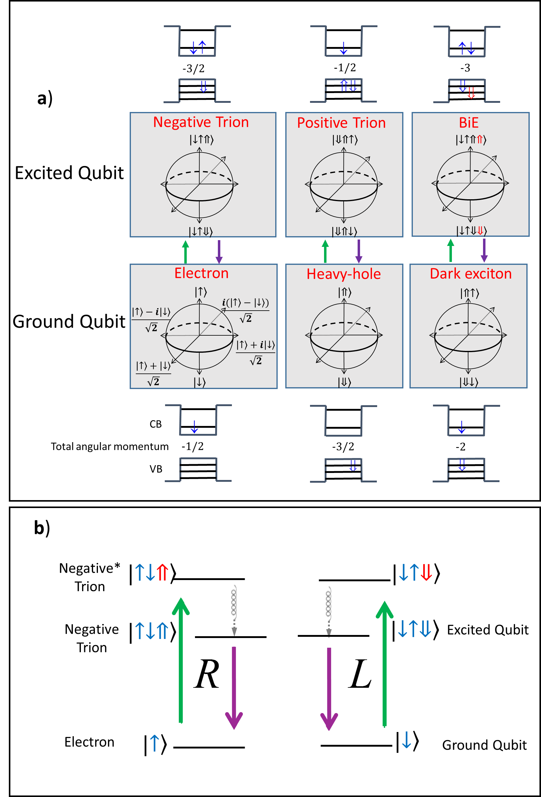
Figure 1: (a) Spin wavefunctions and Bloch-sphere representations of the six matter spin qubits used in this work. The 6 qubits, represented by their Bloch spheres, are divided into 3 pairs of ground and excited level qubits. The spin wavefunctions of the ground- (excited-) level qubits are schematically described below (above) the respective Bloch spheres, where $\uparrow$ ($\Downarrow$) represents spin up electron (down heavy hole), and the blue (red) color represents a carrier in its ground (excited) energy level. Green upward arrows represent laser pulses which convert the ground level qubit to its respective excited level qubit. Magenta downward arrows represent single photons emitted from the excited qubits thereby returning to the ground level qubit. (b) The optical transitions and polarization selection rules for the electron-trion system, which form a ground level–excited level qubit pair. Note that in this example (as in all other cases) an optical $\Pi$-system is described, but the exciting laser pulse is tuned to an excited trion level, in order to facilitate polarization tomography of the emitted photon (magenta downdward arrows) by spectrally separating the emission from the exciting laser pulse (green upward arrows). The fast (~70 ps (Schwartz et al., 2015a)) phonon-assisted relaxation of the excited trion to the ground trion level is represented by gray curly downward arrows. The right (left) hand circular polarization of the photons which connect the $1/2$ ($-1/2$) spin state of the ground level qubit with the $+3/2$ ($-3/2$) spin state of the excited qubit are marked by $R$ ($L$).

At low temperatures and in the absence of external magnetic field, the main decoherence mechanism of these electronic spin qubits is the hyperfine interaction between the electronic (central) spin and the spin of the nuclei of the $\sim 10^{5}$ atoms which form the QDs (Gammon et al., 2001; Merkulov et al., 2002b; Khaetskii et al., 2002). The two types of charge carriers in semiconductors, the negative conduction band electrons, and the positive, valence band holes interact differently with the nuclei, since their orbital momentum around the nucleus is different. The conduction electrons have zero atomic orbital momentum, while valence band holes have unit atomic orbital momentum. Consequently, the conduction electron’s wavefunction strongly overlaps with the nucleus and interacts with the nuclear spin via the Fermi contact interaction. In contrast, the valence hole’s wavefunction vanishes at the nucleus site and therefore its spin interacts with the nuclear spin via the weaker dipole-dipole hyperfine interaction (Fischer et al., 2008). In addition, while the conduction-electron interaction with the nuclei, which we denote by $\gamma_{e}$ is isotropic, the interaction of the valence heavy hole for which the orbital angular momentum and the spin are aligned parallel to the growth direction, is anisotropic. We denote by $\gamma_{h_{z}}$the interaction of the valence heavy-hole spin with the nuclei spin bath along the QD growth axis ($\hat{z}$) and by $\gamma_{h_{p}}$ the interaction with nuclear spins in the plane perpendicular to $\hat{z}$.

The dynamics of the electronic central spin can be divided into two different time domains as schematically described in Fig. 2 a, b and c for the electron, heavy hole and DE spins respectively (Merkulov et al., 2002b).

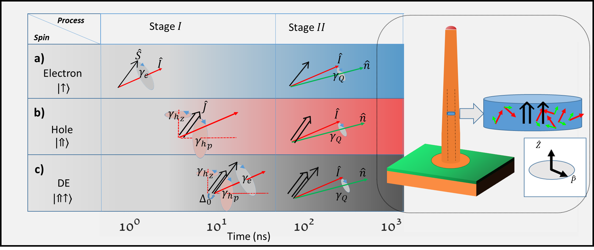
Figure 2: Schematic description of the spin dephasing processes of the QD confined electron (a), heavy-hole (b), and dark exciton (c). Each process is divided into two temporal stages: During the first stage the initiated central spin precesses around the effective magnetic field which results from the frozen fluctuation of the nuclear spins of about $10^{5}$ atoms comprising the QD. The electron spin ($\hat{S)}$ interacts with the nuclear spin ($\hat{I}$) via the isotropic Fermi contact interaction described by $\gamma_{e}$. The heavy-hole spin ($\hat{J)}$ interacts with the nuclear spin via the anisotropic dipole-dipole hyperfine interaction denoted by $\gamma_{h_{z}}$ and $\gamma_{h_{p}}$, where $\hat{z}$ is the QD growth direction and $p$ denotes direction in a plane perpendicular to $\hat{z}$. The dark exciton contains an electron and a heavy hole. Both spins interact with the nuclear spin, and in addition, the electron and hole interact with each other mainly via the isotropic exchange interaction denoted by $\Delta_{0}$ (Bayer et al., 2002). During the second stage the nuclear spins react to strain induced electric fields gradients (EFG) in the QD (Sinitsyn et al., 2012). This interaction has a quadrupole nature, and we denote it by $\gamma_{Q}$. The motion of each nuclear spin is described by an effective local magnetic field in a direction marked by $\hat{n}$ which the nuclear spin slowly precesses around. During the second stage, we use the adiabatic approximation, by which the central spin just follows the slowly varying effective nuclear magnetic field. The various interaction magnitudes are summarized and referenced in Table 1. Inset: schematic description of the InAsP QD (blue) embedded in the InP photonic nanowire (orange). The central spin is represented by the black arrows, the nuclear spin bath are represented by the red arrows, and the EFGs are schematically represented by green arrows in the magnified description of the QD.

During the first stage, the central spin precesses around a mean effective magnetic field generated by the frozen fluctuations of the nuclear spins in its vicinity. The electron interacts with the nuclear field via the isotropic Fermi contact hyperfine interaction marked by $\gamma_{e}$, while the heavy-hole interacts via the anisotropic dipole-dipole hyperfine interaction marked by $\gamma_{h_{z}}$ and $\gamma_{h_{p}}$. As the DE is formed by an electron-hole pair with parallel spins, each of these carriers interacts with the nuclear magnetic field, while at the same time they also interact with each other, via the electron-hole exchange interactions. The most important term in this interaction is the isotropic term $\Delta_{0}$ (Bayer et al., 2002; Ivchenko, 2005), separating the DE and BE (an antiparallel electron-hole pair) energy levels. Being much stronger than the hyperfine interactions it prevents the separate spin flip of either one of the two individual spins and consequently protects the DE spin from dephasing. It turns out, as we show in Appendix B, below, that the DE nuclear field induced dephasing is caused mainly due to small DE-BE mixing terms (of order $10^{-3}$).

During the second stage, at longer times, the fluctuations in the nuclear magnetic field can no longer be considered “frozen” and they slowly evolve in time. This evolution is described as local precession of the effective magnetic field around local directions denoted by $\hat{n}$. A relatively simple model describes this motion as generated by the quadrupole interaction (denoted by $\gamma_{Q}$) of the nuclear spins with the strain induced electric fields gradients in the QD (Sinitsyn et al., 2012; Bechtold et al., 2015). We adopt this description, since it permits analytic solution to the problem, thereby simplifying the comparison with the measured data, while keeping the generality of our approach. Finally, at yet longer times, which is beyond the scope of this work, the nuclei also interact with each other via the dipole-dipole nuclear interaction (Erlingsson and Nazarov, 2004). During the second stage the central spin continues to interact with the slowly varying effective nuclear magnetic field in the same manner as it does during the first stage. Therefore, the central spin dynamics can be described as a sort of “convolution” between the relatively fast dynamics of the spin around the average nuclear magnetic field, with the dynamics of the slowly varying nuclear field.

The details of the model involved in these calculations, which follows references (Merkulov et al., 2002b; Sinitsyn et al., 2012; Bechtold et al., 2015), describing the evolution of the electron, and the generalization of the model to include the heavy-hole evolution, are described in Appendix A. The model which describe the dynamics of the DE is developed in Appendix B.

A great deal of effort was devoted to study the coherence properties of the central electronic spin for both, conduction band electrons (Bluhm et al., 2010; Braun et al., 2005), and valence band heavy-holes (Brunner et al., 2009; Eble et al., 2009; Fras et al., 2011; Li et al., 2012; Gerardot et al., 2008), confined in QDs. The temporal evolution of a single electron spin at vanishing external magnetic field was experimentally measured recently by Bechtold and coworkers (Bechtold et al., 2015). To the best of our knowledge, similar measurements for the heavy-hole as a central spin have not been reported so far. Here, we present comprehensive measurements of the spin depolarization dynamics for both the electron and the heavy hole as well as for their correlated pair – the DE. All these forms of central electronic spin are confined to the same QD. In addition, we show, by measuring the temporal evolution of the positive and negative trions’ spins, that the presence of two additional paired charge carriers, does not affect the central spin depolarization. Our measurements were preformed optically without applying any external magnetic field. In addition, we carried out the experiments in a way which prevented the generation of a steady state nuclear Overhauser field. The experimental methods and measurements are described below and the measured results are compared with the central spin models discussed in the Appendices.

II The device and experimental methods

The InP nanowire containing a single InAsP quantum dot (Dalacu et al., 2009, 2012; Bulgarini et al., 2014) was grown using chemical beam epitaxy with trimethylindium and pre-cracked $\mathrm{PH_{3}}$ and $\mathrm{AsH_{3}}$ sources. The nanowires were grown on a $\mathrm{SiO_{2}}$-patterned (111)B InP substrate consisting of circular holes opened up in the oxide mask using electron-beam lithography and a hydrofluoric acid wet-etch. Gold was deposited in these holes using a self-aligned lift-off process, which allows the nanowires to be positioned at known locations on the substrate. The thickness of the deposited gold is chosen to give 20-nm to 40-nm diameter particles, depending on the size of the hole opening. The nanowires were grown at $420^{\circ}$ C with a trimethylindium flux equivalent to that used for a planar InP growth rate of 0.1 µm/hr on (001) InP substrates at a temperature of $500^{\circ}$ C. The growth is a two-step process: (i) growth of a nanowire core containing the quantum dot, nominally 200 nm from the nanowire base, and (ii) cladding of the core to realize nanowire diameters (around 200 nm) for efficient light extraction. The quantum dot diameters are determined by the size of the nanowire core. The particular QD reported on here has diameter of $\sim 30$ nm.

The sample was placed inside a sealed metal tube cooled by a closed-cycle helium refrigerator maintaining a temperature of 4 K. A ×60 microscope objective with numerical aperture of 0.85 was placed above the sample and used to focus the laser beams on the sample surface and to collect the emitted PL from it. Pulsed laser excitations were used. The picosecond pulses were generated by two synchronously pumped dye lasers at a repetition rate of 76 MHz. The temporal width of the pulses was 12 ps and their spectral width $\sim 100$ µeV. Light from a continuous wave (CW) laser, modulated by an acousto-optic modulator, synchronized with the dye lasers, was used to produce pulses of up to 30 ns duration. These pulses were used to set the average QD charge state (Benny et al., 2012). A second CW laser, modulated by an electro-optic modulator, was used to produce depletion pulses of 30 ns duration (Schmidgall et al., 2015). The timing between the two synchronized ps pulses was controlled using 2 cavity dumpers which effectively reduced the repetition rate down to 0.5 MHz. In addition, a computer controlled motorized delay line was used to finely tune the temporal delay between the pulses. The polarizations of the excitation pulses were independently adjusted using polarized beam splitters (PBS) and two pairs of computer-controlled liquid crystal variable retarders (LCVRs) (Schwartz et al., 2016). The collected PL was equally divided into 2 beams by a non-polarizing beam splitter. Two pairs of LCVRs and a PBS were then used to analyze the polarizations of each beam. This way the emitted PL was divided into four beams, allowing selection of two independent polarization projections and their complementary polarizations. The PL from each beam was spectrally analyzed by either a 1 or 0.5 meter monochromator and detected by a silicon avalanche photodetector coupled to a PicoQuant HydraHarp 400™ time-correlated photon counting and time tagging system, synchronized with the pulsed lasers. This way the arrival times of up to 4 emitted photons have been recorded with respect to the synchronized laser pulses.

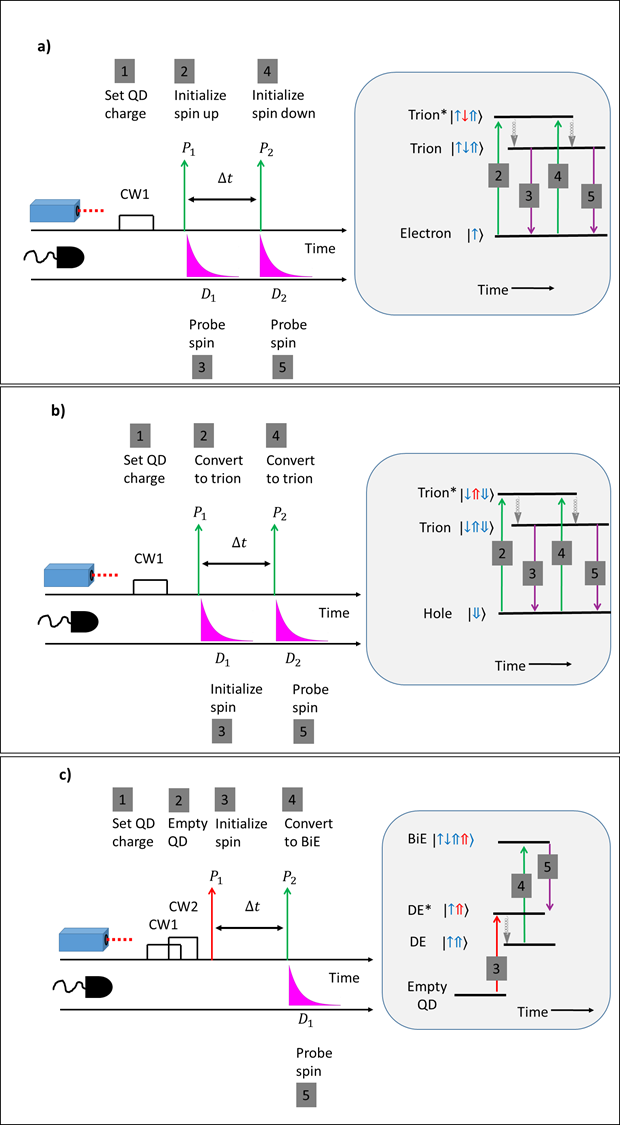
Figure 3: Schematic description of the experiments for measuring the spin dynamics of: a) Positive and negative trions, b) Single electron and single heavy-hole. c) Dark exciton. The optical transitions in each experiment are described by the energy level diagram to the right. The carrier’s spins are marked in the figure using the notations of Fig. 1, where blue (red) color represent ground (excited) single carrier states. CW1 and CW2 represent the 20 ns gated CW laser pulses where $P_{1}$ and $P_{2}$ represent the 12 ps pulses produced by the synchronously pumped and cavity dumped dye lasers. $\Delta t$ is the time delay between the two pulses in each repetition period, controlled by two cavity dumpers and a delay line. $D_{1}$ and $D_{2}$ represent the emission and time resolved detection of the two single photons emitted as a result of the $P_{1}$ and $P_{2}$ excitations.

We used the optical transitions between the ground level qubits and the excited level qubits to initialize the spin state of both qubits, and then for probing the spin state of the qubits at a later time. We facilitate the optical transition selection rules of the $\Pi$-systems described in Fig. 1b in order to do that.

For initializing the excited qubit, one simply applies an $R$ or $L$ polarized $\pi$-pulse. For probing the excited qubit spin projection, one simply measures the degree of circular polarization of the emitted photons $\hat{S}_{z}=\left(I_{R}-I_{L}\right)/\left(I_{R}+I_{L}\right)$ where $I_{R(L)}$ is the measured emission intensity projected on right (left) hand circular polarization.

The initialization of the ground level qubit is provided by detecting $R$ or $L$ polarized single photon, which heralds the spin state of the qubit at the photon emission time. Probing the ground level qubit spin state is done by first converting the state into the state of the excited level qubit, using an horizontally linearly polarized ($H=\left(R+L\right)/\sqrt{2}$) $\pi$-pulse, and then measuring the time resolved degree of circular polarization of the emitted photons. For example, in Fig. 1(b) if the electron spin state before the pulse is described by: $\hat{\rho}_{\mathrm{electron}}=p\left|\Psi_{\mathrm{electron}}\right\rangle\left\langle\Psi_{\mathrm{electron}}\right|$+$\left(1-p\right)\frac{1}{2}\mathbb{I}$, where $\mathbb{I}$ is the identity matrix and $p$ is the probability of $\hat{\rho}_{\mathrm{electron}}$ being in a pure state $\left|\Psi_{\mathrm{electron}}\right\rangle=\alpha\left|\uparrow\right\rangle+\beta\left|\downarrow\right\rangle$, then after the pulse the photogenerated trion spin state is given by: $\hat{\rho}_{\mathrm{trion}}=p\left|\Psi_{\mathrm{trion}}\right\rangle\left\langle\Psi_{\mathrm{trion}}\right|$+$\left(1-p\right)\frac{1}{2}\mathbb{I}$, with $\left|\Psi_{\mathrm{trion}}\right\rangle=\alpha\left|\uparrow\downarrow\Uparrow\right\rangle+\beta\left|\downarrow\uparrow\Downarrow\right\rangle$, with the same $\alpha$, $\beta$ and $p$. Here, we assume of course, that the fidelity of the optical excitation by the $H$ polarized $\pi$-pulse is unity and that the experimental deviation from truly $H$ polarization is negligible. The spin projection of excited qubit on the $\hat{z}$-direction is then deduced by measuring the degree of circular polarization of the emitted photons.

We conducted 5 different experiments in order to comprehensively study the central spin dynamics for various confined spin qubits in the QD. In the first 2 measurements, schematically described in Fig. 3a, we measured the depolarization of the negative or positive trions. We first pump the QD to either a negative or a positive charge state by using above bandgap CW1 pulse of about 10ns duration(Benny et al., 2012). Then, either an excited negative or positive trion was photogenerated by using a short circularly polarized quasi-resonant ~12 ps long laser pulse. The polarization of the excitation pulse determines the spin polarization of the minority carrier in the initialized trion [hole (electron) in the negative (positive) trion]. After a fast (~70 ps (Schwartz et al., 2015a)) spin preserving phonon assisted relaxation of the excited trion, a ground level trion is formed. When the trion decays radiatively, the polarization of the emitted photon reflects the spin of the minority carrier at the particular time in which the photon is emitted. Thereby, by using time resolved circular polarization sensitive PL measurements we probe the spin relaxation dynamics of the minority carrier in the trion. This technique provides a simple way of measuring the dynamics of the spin of the confined electron (hole) in the presence of a spin singlet pair of two holes (electrons). Unfortunately, this simple method is limited by the relatively short radiative lifetime of the trion. Only the evolution during the first time domain can be measured this way. In order to avoid generating a steady state Overhauser field in the QD due to the repeated circularly polarized quasi-resonant excitation pulse, a second pulse with opposite circular polarization is used to re-excite the trion a few ns after the first pulse, during the same excitation period. The time resolved degree of circular polarization was deduced using the resulted PL from both complementary pulses.

The measurement of the spin dynamics of either the single electron or heavy-hole was carried out using the same experimental system but at somewhat different manner, as schematically described in Fig. 3b. In the inset to this figure we describe the energy levels of the heavy-hole system. Here, after the optical charging, a trion was generated by quasi resonant excitation using a horizontal ($H$) polarized pulse. Either the electron or the hole spin was initialized by detecting the circular polarization of the emitted single photon. In order to probe the temporal dependence of the spin state of the carrier, a second, horizontal polarized delayed 12 ps pulse is used to re-excite the carrier to its respective trion and the resulting circular polarization of the emitted photon is used to measure the spin polarization of the carrier at the re-excitation time. This measurement is not limited by the radiative lifetime of the trion, however, it requires two-photon intensity correlation measurements in a relatively slow repetition rate (~500 kHz). We achieved this low repetition rate by using the cavity dumpers. The feasible maximal delay time (~1 µs$)$ between the pulses was defined by the rejection ratio (of about $\sim 2\vartimes 10^{-3}$ ) of neighboring pulses of the cavity dumpers. Note that in these experiments the generation of an Overhauser field is avoided because the initialization of the central spin is not done deterministically by using circularly polarized excitation, but rather probabilistically by post-selecting the detected circular polarization of the emitted first photon.

The spin dynamics of the DE was probed as schematically described in Fig. 3c. Here, we used above-bandgap optical pumping of about 20 ns to neutralize the QD and then another quasi-resonant pumping of about 20 ns to deplete the QD from the DE (Schmidgall et al., 2015). After depleting the QD, a quasi-resonant circularly polarized 12 ps pulse initialized the DE in spin up excited state (Schwartz et al., 2015b). Following this initialization, the DE relaxes to its ground state within ~70 ps by spin-preserving emission of a phonon. In order to probe the DE state, a delayed, linearly polarized resonant 12 ps pulse converted the DE qubit into the BiE qubit. Note that the horizontal polarization of the laser preserves the phase of the qubit. The detection of a circularly polarized photon, which results from the radiative recombination (~1 ns lifetime) of the BiE is then used to probe the spin state of the DE in the QD, at the converting pulse time. Repetition rates as low as ~500 kHz, allow temporal delays of over 1 µs between initialization and probing of the spin. In this experimental method an Overhauser field is not generated in the sample since the gated CW pulses used to optically pump and deplete the QD are linearly polarized.

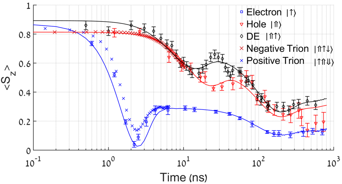
Figure 4: Measured central spin polarization $\left\langle S_{z}\right\rangle$ as a function of time after its initialization, for the QD confined electron (blue square symbols), heavy-hole (red triangle symbols), dark exciton (black diamond symbols), negative trion (red $\times$symbols), and positive trion (blue $\times$ symbols). Error bars represent one standard deviation of the experimental uncertainty. Solid color matched lines represent the fitted theoretical model (see appendices), for each case. The spin wavefunctions are schematically described in the legend, where the notations of Fig. 1 are used.

III Results and discussion

In Fig. 4 we present the measured degree of the average central spin polarization $\left\langle S_{z}(t)\right\rangle$ as a function of time after its initialization, for the 5 spin qubits: the conduction band electron, the valence band heavy-hole, the positive and negative trions, and the dark exciton. The error bars represent one standard deviation of the experimental uncertainty. At time zero the central spin is initialized to spin-up state. Then, the projection of the spin on $\hat{z}$ direction (the QD growth axis) is displayed as a function of time.

The conduction band electron spin state (blue rectangles) depolarizes from its initial state within ~2 ns. The spin polarization then revives to about a third of the initial polarization. From this level the polarization continues to decay at a much slower rate, reaching a second minimum at about ~200 ns. Afterwards the spin polarization revives again to about 10% of the initial polarization. This behavior is similar to that reported in Ref. (Bechtold et al., 2015), as predicted by Ref. (Merkulov et al., 2002b). Roughly speaking, the first fast dephasing step is a measure for the strong Fermi-contact hyperfine interaction of the electron with the nuclear spin bath, while the second step measures the strength of the quadrupole interaction of the nuclear spin bath with the strain induced electric field gradients in the QD.

After initialization, the heavy-hole (red triangles) spin depolarizes in about an order of magnitude slower than the electron spin. This is due to the much weaker dipole-dipole hyperfine interaction. The hole spin polarization decreases at about ~20 ns to about one half of its initial polarization. Afterwards it mildly revives followed by a slow decay due to the quadrupole interaction of the nuclear bath.

The positive trion spin polarization (blue $\times$ symbols), behaves similarly to that of the electron, while the negatively charged trion spin polarization (red $\times$ symbols) follows that of the heavy-hole. This is not surprising, since the trion polarization reflects the polarization of the unpaired minority carrier, in the presence of the two paired majority carriers. As explained above, the trions spin measurements are limited by their radiative lifetime of about ~1 ns.

The dark exciton (black diamonds) decoheres slowly, in a similar rate to the heavy-hole. However, like the electron, after the initial decay, it strongly revives to about two thirds of its initial polarization. This is due to the strong exchange interaction between the electron and hole that protects both carriers from flipping their individual spins. Later, after ~200 ns the dark exciton polarization continues to decay due to the quadrupole interaction.

We fit the measured temporal behavior of the electron, heavy hole and dark exciton using one conceptually simple central spin model. For the fitting, only five free parameters are used: 1) The hyperfine Fermi-contact interaction $\gamma_{e}$, 2) the heavy-hole out-of-plain hyperfine dipole-dipole interaction $\gamma_{h_{Z}}$, 3) the heavy-hole in-plain hyperfine dipole-dipole interaction $\gamma_{h_{p}}$, 4) the DE in-plane interaction $\gamma_{\mathrm{DE}_{p}}$ and 5) the quadrupole interaction $\gamma_{Q}$. These parameters are accurately defined in the appendices, where the models are discussed for the electron and the heavy-hole (Appendix A), and for the DE (Appendix B).

The best fitted parameters are given in Table I, where they are also compared with the available literature. Our analysis provides an estimation of the number of atoms in the QD: $N_{L}=3\cdot 10^{5}.$ With this estimation our fitted hyperfine Fermi contact $\gamma_{e}$ is comparable to that of Ref. (Gotschy et al., 1989).

Characteristic spin depolarization times during the first and second temporal stages can be obtained from our fitting procedure quite straightforwardly. Since the central spins in this work are initialized in z direction, depolarization is caused by the in-plane interaction parameters. Thus, the temporal location of the first minimum is a rough measure of the in-plane interaction parameter: $T_{\min}=\hbar/\gamma_{{}_{p}}\sim 2$, 20 and 14 ns for the electron, heavy-hole and DE, respectively. Thus, $\gamma_{e}$, $\gamma_{h_{p}}$ and $\gamma_{\mathrm{DE}_{p}}$ are given by $0.34,$ $0.031$ and $0.047\,\text{\textmu eV}$, respectively.

The central spin interaction with the nuclear field along the $z$-direction, acts as a restraining force, which actually prolongs the spin coherence. Therefore, roughly speaking, the ratio between these interactions ( $R_{\gamma}=\gamma_{{}_{Z}}/\gamma_{{}_{P}})$ determines the depth of the first polarization minimum and the maximum value of the polarization after its revival. We thus obtain $R_{\gamma}$=1, 3.5 and 5, for the electron, hole and DE, respectively. Note that for the electron the ratio is by definition 1, and therefore the polarization degree revives to 1/3 of its initial value, while for the hole and DE it revives to higher values. During the second temporal stage, the polarization of all three central spins decays more or less at the same rate, determined by the quadrupole interaction $\gamma_{Q}$. Therefore the temporal location of the second minimum is about the same in all cases given by $T_{\min_{Q}}=\hbar/\gamma_{Q}\sim 200\,\mathrm{ns}$ or $\gamma_{Q}\sim 0.003\,\text{\textmu eV}$.

A common practice for quantifying the depolarization value of a spin qubit is to define the depolarization time as the time it takes for the polarization to reduce to 1/e of its initial state. We adopt this practice, though the measured depolarizations are clearly non-exponential. The measured depolarization times thus obtained are $1.5$, $130$ and $145$ ns for the electron, heavy hole and DE respectively.

Table 1: The various interaction energies as obtained by the best model fitting to the measured temporal depolarization of five different electronic spin qubits confined in the same QD. The theoretical model and the fitted parameters are described in the text and the Appendices.

Interaction	This work (µeV)	Literature (µeV)
$\gamma_{e}\,$	$0.34\pm 0.03$	$0.33$ (Bechtold et al., 2015)
$\gamma_{h_{z}}\,\,$	$0.11\pm 0.03$	$0.081$ (Eble et al., 2009)
$\gamma_{h_{p}}\,\,$	$0.031\pm 0.006$	$0.047$ (Eble et al., 2009)
$\gamma_{\mathrm{DE}_{p}}\,\,\,$	$0.047\pm 0.006$	—–
$\gamma_{Q}\qquad$	$0.0031\pm 0.001$	$0.00087$ (Bechtold et al., 2015)

IV Summary

We investigated both experimentally and theoretically the depolarization dynamics of five different electronic spin configurations confined in the same semiconductor quantum dot. Our measurements were carried out all optically and in the absence of externally applied magnetic field. We show that the measured temporal spin depolarization is well described by a central spin model which attributes the depolarization to the hyperfine interaction between the electronic spin and the nuclear spin bath of the QD atoms.

We divide the depolarization into two temporal stages. During the initial stage the central spin precesses around the effective magnetic fields of the frozen fluctuations of the $10^{5}$ nuclear spins in the QD. During the second stage the central spin precession follows adiabatically the nuclear spin bath dynamics which ceases to be frozen and effectively precesses around strain induced electric fields gradients in the QD.

These two processes result in a relatively fast initial depolarization of the central spin reaching a first minimum. The depolarization minimum is then followed by a temporal revival of the polarization degree and finally by a second depolarization reaching a minimum at a much later time which is more or less equal for all the electronic central spin cases.

Our model assumes that while the hyperfine interaction between the central spin and the nuclear spins is isotropic for the electron, it is anisotropic for the heavy-hole and therefore also for the DE, which is formed by an electron–heavy-hole pair. The depolarization times that we measured in zero magnetic field show that the electron depolarizes much faster than the heavy-hole This observation is explained by the difference between the strong isotropic electron-nucleous hyperfine contact interaction ($\gamma_{e}$ ) and the anisotropic hole-nucleous dipolar hyperfine interactions ($\gamma_{h_{Z}},\gamma_{h_{p}}$). The heavy hole spin depolarizes faster than the dark exciton spin due to the electron-hole exchange interaction, which protects the dark-exciton spin from depolarizing. The depolarization of the dark-exciton results from residual dark exciton–bright exciton mixing. We believe that this mixing can be significantly reduced by increasing the QD symmetry and by avoiding alloying. In this case the dark-exciton may form an almost non-dephasing electronic spin qubit in a semiconductor environment.

V Acknowledgement

The support of the Israeli Science Foundation (ISF), and that of the European Research Council (ERC) under the European Union’s Horizon 2020 research and innovation programme (grant agreement No 695188) are gratefully acknowledged.

Appendix A Hyperfine interaction of the electron and the heavy-hole

We outline here a model for describing the temporal evolution of the QD confined central spin polarization in the absence of externally applied magnetic field but in the presence of effective magnetic field generated by the nuclear spins, which comprise the QD. As the central spin we consider either the electron or the heavy hole. We then apply the same model also to a central spin formed by the DE – a long lived electron–heavy-hole pair, as will be discussed in Appendix B.

As all three cases involve a two level system (a qubit) they may be described using the Pauli matrices $\sigma_{x},\sigma_{y},\sigma_{z}$ and the effective Hamiltonian must take the form

$$H=\frac{1}{2}\vec{C}\cdot\vec{\sigma},$$

for some $\vec{C}=(C_{x},C_{y},C_{z})$. The exact expression of $\vec{C}$ will be different, of course, for each type of central spin.

The hyperfine Fermi-contact interaction between an electron and all the nuclei in the QD is given by (Merkulov et al., 2002b) :

$$H=\frac{\nu_{0}}{2}\sum|\psi_{\mathrm{env}}(\vec{r}_{i})|^{2}A_{e}^{i}\vec{I}_{i}\cdot\overrightarrow{\sigma}.$$

Here $\nu_{0}$ is the volume of the unit cell, $\vec{r}_{i}$ and $\vec{I}_{i}$ are the ith nucleus position and its spin operator, $\psi_{\mathrm{env}}(\vec{r})$ describes the electron envelope wavefunction and $A_{e}^{i}$ is an effective hyperfine interaction constant between the electron and the specific nucleus in the $\vec{r}_{i}$ position where the index i runs over all the nuclei in the QD. Since $A_{e}^{i}$ depends on the atomic nuclear spin it is much larger for indium atoms than for all other atoms in the QD. Thus, in principle, one can neglect other nuclei contributions. We proceed by defining an expression for the effective magnetic field, which the nuclei apply on the electron. The field, known also as the Overhauser field, is defined as:

$$\vec{B}_{N}=\frac{1}{g_{e}\mu_{B}}\vec{C}_{e}=\frac{\nu_{0}}{g_{e}\mu_{B}}\sum A_{e}^{i}|\psi_{\mathrm{env}}(\vec{r}_{i})|^{2}\left\langle\vec{I}_{i}\right\rangle_{N},$$

where $g_{e}$ and $\mu_{B}$ are the electron g-factor and Bohr magneton respectively, and $\left\langle...\right\rangle_{N}$ denotes a quantum mechanical average over the nuclear spins which interact with the electron.

Assuming that different nuclear spins are not correlated allows one to treat $\vec{B}_{N}(t)$ as having isotropic Gaussian random distribution satisfying

$$\langle\vec{B}\rangle=0,\quad\langle B_{Nx}^{2}\rangle=\langle B_{Ny}^{2}\rangle=\langle B_{Nz}^{2}\rangle=\sigma^{2},$$

where the width of the distribution $\sigma$ is given by (Merkulov et al., 2002b)

$$3\sigma^{2}=\sum\frac{(A_{e}^{i})^{2}}{\mu_{B}^{2}g_{e}^{2}}\nu_{0}^{2}|\psi_{\mathrm{env}}(\vec{r}_{i})|^{4}I_{i}(I_{i}+1).$$

It is then convenient to define a modified unitless magnetic field $\vec{\tilde{B}}=\frac{1}{\sigma}\vec{B}_{N}$. In the following we simply mark this modified Overhauser field as $\vec{B}$. The electron spin Hamiltonian can then be expressed by $H=\frac{1}{2}\vec{C}_{e}\cdot\vec{\sigma}$ with $\vec{C}_{e}=\gamma_{e}\vec{B}$ where $\gamma_{e}=g_{e}\mu_{B}\sigma$ is the electron coupling constant in energy units, which we use as a fitting parameter.

While for the electron, $s$-wave molecular symmetry results in a scalar effective coupling $A_{e}^{i}$, for the heavy hole it is described by an anisotropic tensor

$$\hat{A}_{h}^{i}=\left(\begin{array}[]{ccc}A_{h,p}^{i}\\ &A_{h,p}^{i}\\ &&A_{h,z}^{i}\end{array}\right).$$

Where the in plane dipole-dipole interaction constant $A_{h,p}^{i}$ does not strictly vanish for the heavy-hole due to mixing with the light-hole (Eble et al., 2009). Therefore, for the heavy-hole we define $C_{z}=\gamma_{h_{z}}B_{z},C_{x,y}=\gamma_{h_{p}}B_{x,y}$ where $\gamma_{h_{z}}>\gamma_{h_{p}}$, are also fitting parameters. Strictly speaking, the field $\vec{B}$ appearing here is not exactly the same one as in the electron case. This is due to differences in relative weighting of various nuclei between electron and hole wavefunctions. For our purpose, however, it is sufficient that the fields have the same Gaussian statistics. For the moment we allow the functional relation between $\vec{C}$ and $\vec{B}$ to be arbitrary and since our discussion is independent of these relations, it applies to all three cases.

At short times $\vec{B}$ and hence also $\vec{C}$ can be treated as time independent and one readily find the solution

$$\vec{S}(t) =\frac{\vec{S}_{0}\cdot\vec{C}}{C^{2}}\vec{C}+\left(\vec{S}_{0}-\frac{\vec{S}_{0}\cdot\vec{C}}{C^{2}}\vec{C}\right)\cos\left(\frac{C}{\hbar}t\right)$$ (1)

$$-\frac{\vec{S}_{0}\times\vec{C}}{C}\sin\left(\frac{C}{\hbar}t\right),$$

where $\vec{S}_{0}=\vec{S}(0)$ is the central spin initial value. The first term is time independent and survives for long times. Upon averaging over the random ensemble of possible $\vec{C}$s one typically finds that the oscillating terms turn into exponentially decaying transients, relevant at short times only. In practice the last term usually vanishes by symmetry under $\vec{C}\rightarrow-\vec{C}$. In particular it applies to our experiments, which were carried out in the absence of externally applied magnetic field. Therefore, in the following we disregard this term.

At longer times, we use the adiabatic approximation and assume that the central spin follows the direction of $\vec{C}$, while the rapidly rotating components orthogonal to $\vec{C}$ average to zero. We can therefore write

$$\vec{S}(t)=\left(\vec{S}_{0}\cdot\hat{C}(0)\right)\hat{C}(t)=\frac{\vec{S}_{0}\cdot\vec{C}(0)}{C(0)C(t)}\vec{C}(t).$$ (2)

For small $t$ this clearly coincides with the first term of Eq. (1). As the other terms of Eq. (1) vanish at long times one sees that the two relations Eqs. (1,2) can be combined into an expression which applies at arbitrary time $t$:

$$\vec{S}(t) =\frac{\vec{S}_{0}\cdot\vec{C}(0)}{C(0)C(t)}\vec{C}(t)$$ (3)

$$+\left(\vec{S}_{0}-\frac{\vec{S}_{0}\cdot\vec{C}(0)}{C(0)^{2}}\vec{C}(0)\right)\cos\left(\frac{C(0)}{\hbar}t\right).$$

The Gaussian probability density corresponding to the dimensionless Overhauser field at a given moment is given by

$$dP_{1}=\frac{1}{(2\pi)^{3/2}}\exp\left(-\frac{1}{2}B^{2}\right)d^{3}B.$$ (4)

Assuming further that

$$\langle B_{i}(t_{1})B_{j}(t_{2})\rangle=\delta_{ij}f(t_{2}-t_{1})$$

(Consistency requires $f(0)=1$) we can write the joint probability density of $\vec{B}_{1}=\vec{B}(0)$ and $\vec{B}_{2}=\vec{B}(t)$ as

$$dP_{2} =\frac{d^{3}B_{1}d^{3}B_{2}}{\left(2\pi\sqrt{1-f(t)^{2}}\right)^{3}}$$

$$\exp\left[-\frac{1}{2}\left(B_{1}^{2}+B_{2}^{2}-2f(t)\vec{B}_{1}\cdot\vec{B}_{2}\right)/(1-f(t)^{2})\right].$$ (5)

Using the probability distributions Eqs. (4,5) we can write the average central spin evolution as

$$\langle\vec{S}(t)\rangle =\int\frac{\vec{S}_{0}\cdot\vec{C}(0)}{C(0)C(t)}\vec{C}(t)\,dP_{2}$$

$$+\int\left(\vec{S}_{0}-\frac{\vec{S}_{0}\cdot\vec{C}}{C^{2}}\vec{C}\right)\cos\left(\frac{C}{\hbar}t\right)dP_{1}$$ (6)

Actual computation of the integrals requires using the specific functional relation between $\vec{B}$ and $\vec{C}$.

For the electron as the central spin, we simply substitute $\vec{C}=\gamma_{e}\vec{B}$ and $\vec{S}_{0}=\hat{z}$ in Eq. (6) and obtain integrals which can be evaluated analytically (Merkulov et al., 2002b; Bechtold et al., 2015), resulting in

$$\langle S_{z}\rangle =\frac{2}{3}\left(1-\left(\frac{\gamma_{e}t}{\hbar}\right)^{2}\right)e^{-\frac{1}{2}\left(\frac{\gamma_{e}t}{\hbar}\right)^{2}}$$

$$+\frac{2}{3\pi}\left(\sqrt{\frac{1}{f(t)^{2}}-1}+\left(2-\frac{1}{f(t)^{2}}\right)\arcsin(f(t))\right).$$

For the heavy-hole as the central spin we have $C_{z}=\alpha B_{z},\;\;C_{x,y}=\beta B_{x,y}$ with $\alpha=\gamma_{h_{z}}$ $\beta=\gamma_{h_{p}}$ In this case $\langle S_{z}\rangle$ is given according to Eq. (6) by a sum of two rather complicated integrals. The second term of Eq. (6) can be reduced into a one-dimensional (1D) integral which we than calculate numerically

$$\frac{\beta^{2}}{\left(\alpha^{2}-\beta^{2}\right)^{3/2}}\int_{\beta}^{\alpha}d\xi\,\frac{(\alpha^{2}-\xi^{2})(1-\sigma^{2}\xi^{2}t^{2})}{\xi\sqrt{\xi^{2}-\beta^{2}}}e^{-\frac{1}{2}\sigma^{2}\xi^{2}t^{2}}.$$ (7)

The first term of Eq. (6) is a more complicated 6D integral. If we use the following shorthands

$$a_{0}=\sqrt{\left(\frac{\cos^{2}\theta}{\alpha^{2}}+\frac{\sin^{2}\theta}{\beta^{2}}\right)\left(\frac{\cos^{2}\theta^{\prime}}{\alpha^{2}}+\frac{\sin^{2}\theta^{\prime}}{\beta^{2}}\right)},$$

$$a_{1}=f(t)\left(\frac{\cos\theta\cos\theta^{\prime}}{\alpha^{2}}+\frac{\sin\theta\sin\theta^{\prime}}{\beta^{2}}\cos\varphi\right),$$

$$A_{0}=\frac{(1-f(t)^{2})^{3/2}}{4\pi^{2}\alpha^{2}\beta^{4}}\sin(2\theta)\sin(2\theta^{\prime})$$

then the 6D integral can be reduced into a 3D one

$$\int_{0}^{2\pi}d\varphi\int_{0}^{\pi/2}d\theta\int_{0}^{\pi/2}d\theta^{\prime}\,A_{0}\biggl{[}\frac{3a_{1}}{(a_{0}^{2}-a_{1}^{2})^{2}}$$

$$+\frac{a_{0}^{2}+2a_{1}^{2}}{(a_{0}^{2}-a_{1}^{2})^{5/2}}\arcsin(a_{1}/a_{0})\biggr{]},$$ (8)

which we than calculate numerically. The function $f(t)$ is essentially the Overhauser field time correlator. An appropriate model for the evolution of the Overhauser field is required for its evaluation.

By using $\vec{B}=\frac{\nu_{0}}{g_{e}\mu_{B}\sigma}\sum A_{i}|\psi_{env}(\vec{r}_{i})|^{2}\vec{I}_{i}$ one obtains:

$$3\sigma^{2}f(t) =\langle\vec{B}(0)\cdot\vec{B}(t)\rangle$$

$$= \sum\left(\frac{\nu_{0}}{g_{e}\mu_{B}\sigma}A_{i}^{2}|\psi_{\mathrm{env}}(\vec{r}_{i})|^{2}\right)^{2}\langle\vec{I}_{i}(0)\cdot\vec{I}_{i}(t)\rangle.$$

A particularly simple model assumes that the Overhauser field evolution is dominated by the quadrupole interaction of the nuclear spins (Sinitsyn et al., 2012; Bechtold et al., 2015). Though more complicated models exist as well (Merkulov et al., 2002b; Bechtold et al., 2015; Al-Hassanieh et al., 2006), this model permits analytical solutions.

Within this model each nuclear spin $\vec{I}_{k}=\vec{I}$ evolves independently of the others by a Hamiltonian of the form $H_{Q}=V_{ij}I_{i}I_{j}$ with random $V_{ij}=V_{ji}$ which relates to the local electric field gradients (Sinitsyn et al., 2012) (EFG). We take the initial state of the nuclear spin to be random and we average over the corresponding wave function thereby obtaining

$$\langle\vec{I}(0)\cdot\vec{I}(t)\rangle\propto\operatorname{Tr}\left(\vec{I}\cdot e^{iH_{Q}t}\vec{I}e^{-iH_{Q}t}\right)$$

As different nuclear spins have different EFG we obtain the Overhauser-correlator $f(t)$ by averaging over the$V_{ij}$ terms. We take (as common in random matrix theory) the elements of the symmetric matrix $V_{ij}$ to be independent Gaussian random variables of variance $\gamma_{Q}^{2}$. Up to overall normalization we obtain

$$f(t)\propto\int dV\,e^{-TrV^{2}/(2\gamma_{Q}^{2})}\operatorname{Tr}\left(\vec{I}\cdot e^{iH_{Q}t}\vec{I}e^{-iH_{Q}t}\right).$$

Noting that $V$ can be taken as a traceless tensor and in addition using its polar decomposition reduce the above expression into a two-dimensional integral which we express as

$$f(t) \propto\int dx_{1}dx_{2}dx_{3}\,\delta\left(\sum x_{i}\right)\prod_{i<j}|x_{i}-x_{j}|e^{\frac{-(x_{1}^{2}+x_{2}^{2}+X_{3}^{2})}{2\gamma_{Q}^{2}}}$$

$$\cdot\operatorname{Tr}\left(\vec{I}\cdot e^{i\sum x_{i}I_{i}^{2}t}\vec{I}e^{-i\sum x_{i}I_{i}^{2}t}\right).$$

For $I=\frac{3}{2}$ we evaluate this expression and obtain:

$$f_{\frac{3}{2}}(t)\propto\int_{0}^{\infty}dx\,x^{4}\,e^{-x^{2}/(2\gamma_{Q}^{2})}(3+2\cos(\sqrt{6}xt))$$

$$f_{\frac{3}{2}}(t)=\frac{3}{5}+\frac{2}{5}\left(1-2\left(\frac{\gamma_{Q}t}{\hbar}\right)^{2}+12\left(\frac{\gamma_{Q}t}{\hbar}\right)^{4}\right)e^{-3\left(\frac{\gamma_{Q}t}{\hbar}\right)^{2}}.$$ (9)

For higher values of the nuclear spin $I$, we calculated $f_{I}(t)$ numerically as a function of the dimensionless product $\gamma_{Q}t/\hbar$. This gave qualitatively similar result to Eq. (9) with some modifications. Since our QD contains $I=\frac{3}{2}$ , $I=\frac{9}{2}$ and $I=\frac{1}{2}$ we averaged over these values using the relative nuclear abundance multiplied by the squared nuclear moments as weights. In Fig. 5 we display the normalized Overhauser-correlator for various types of nuclear spins in the QD. For simplicity we assume the same $\gamma_{Q}$ for all atom types. In practice the Indium contribution dominates the average due to its large magnetic moment.

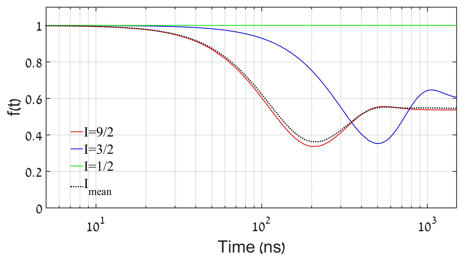
Figure 5: The calculated normalized Overhauser-correlator $f_{I}(t)$ for the various types of nuclear spins which comprise the QD. $I_{\mathrm{mean}}$ is the mean value of the correlator taking into account the isotopic abundances weighted by their squared magnetic moments.

———

Appendix B Hyperfine interaction of the dark exciton.

The spin projection ($S_{z}(t)$) of the DE strongly depends on the electron-hole exchange interaction.

We describe the DE qubit by its two spin states: $|\Uparrow\uparrow\rangle$ and $|\Downarrow\downarrow\rangle$ , with $J_{z}=+2$, and -2 respectively. While the DE interaction with the z-component $B_{z}$ of the Overhauser field is similar to that of a spin $\frac{1}{2}$ central spin (up to multiplicative constant (Bayer et al., 2002)), its interaction with the $B_{x,y}$ components is very different. Strictly speaking, a standard $\vec{B}\cdot\vec{J}$ Hamiltonian would have to act four times in order to flip a $J_{z}=2$ state into $J_{Z}=-2$ state. However, if one fully considers the electron-hole exchange interaction, this is not the case. In the bright and dark excitons basis $\{|\Uparrow\downarrow\rangle,|\Downarrow\uparrow\rangle,|\Uparrow\uparrow\rangle,|\Downarrow\downarrow\rangle\}$ , the exchange interaction can be expressed as (Bayer et al., 2002; Don et al., )

$$\frac{1}{2}\left(\begin{array}[]{cccc}\Delta_{0}&\Delta_{1}^{*}&\Delta_{3}&\Delta_{4}\\ \Delta_{1}&\Delta_{0}&-\Delta_{4}^{*}&-\Delta_{3}^{*}\\ \Delta_{3}^{*}&-\Delta_{4}&-\Delta_{0}&\Delta_{2}^{*}\\ \Delta_{4}^{*}&-\Delta_{3}&\Delta_{2}&-\Delta_{0}\end{array}\right),$$

where $\Delta_{0}$ is the isotropic exchange interaction. It is a real number, which defines the energy splitting between the DE and BE eigenstates. It was measured to be $\Delta_{0}$=260 µeV for the QD under study. The term

$$\Delta_{1}=\delta_{1}\exp(i2\theta_{1})$$

is the anisotropic long-range exchange interaction. Here $\delta_{1}$ is a positive number defining the magnitude of the bright exciton (BE) fine structure splitting (FSS) (Ivchenko, 2005), and $\theta_{1}$ defines the directions of the two cross linearly polarized components of the BE spectral lines with respect to the crystallographic directions (Bayer et al., 2002).

$$\Delta_{2}=\delta_{2}\exp(i2\theta_{2})$$

describes the FSS of the dark exciton. Here $\delta_{2}$ and $\theta_{2}$ are real numbers mainly given by the short range anisotropic exchange interaction.

$$\Delta_{3}=\delta_{3}\exp(i2\theta_{3})$$

and

$$\Delta_{4}=\delta_{4}\exp(i2\theta_{4})$$

are also long-range exchange interactions that couple between the DE and BE states.

Strictly speaking, for a $C_{3v}$ symmetrical QD, $\delta_{1}$, $\delta_{2}$, $\delta_{3}$ and $\delta_{4}$ are all expected to vanish (Dupertuis et al., 2011). To within our experimental uncertainty, we found it to be true only for $\delta_{2}(<0.1\,\text{\textmu eV}$), since it results from the short range exchange interaction and therefore affected mainly by the symmetry of the QD’s unit cells (Bayer et al., 2002). Structural deviations of the QD from symmetry such as composition fluctuations, or faceting, destroy the QD long range symmetry, without affecting its unit cell symmetry. Therefore, they will result in finite $\delta_{1}$ , $\delta_{3}$ and $\delta_{4}$. Indeed, we measured $\delta_{1}=18\,\text{\textmu eV}$ by polarization sensitive spectroscopy, and estimated $\delta_{3}\backsimeq\delta_{4}\backsimeq 15\,\text{\textmu eV}$ by measuring the DE radiative lifetime, and verifying the fact that the DE weak absorption line was linearly polarized in-plane (Schwartz et al., 2015a) .

Since $|\Delta_{3}|=|\Delta_{4}|$$\neq 0$ , these terms induce coupling between the DE and BE states. We define $\left(\Delta_{3}+\Delta_{4}\right)/2\triangleq\Delta_{\mathrm{DB}}$, and since $|\Delta_{\mathrm{DB}}|\ll\Delta_{0}$ , the modified DE eigenstates remain almost degenerate such that the symmetric and anti-symmetric spin combinations are expressed as

$$\left|\mathrm{DE}_{AS}\right\rangle =N_{AS}\left[\frac{\left|\Uparrow\uparrow\right\rangle-\left|\Downarrow\downarrow\right\rangle}{\sqrt{2}}-\frac{\Delta_{\mathrm{DB}}}{\Delta_{0}}\frac{\left|\Uparrow\downarrow\right\rangle+\left|\Downarrow\uparrow\right\rangle}{\sqrt{2}}\right]$$

$$\left|\mathrm{DE}_{S}\right\rangle =\frac{\left|\Uparrow\uparrow\right\rangle+\left|\Downarrow\downarrow\right\rangle}{\sqrt{2}},$$

where $N_{AS}\sim 1$ is a normalization constant. This also agrees with the experimental observation that the DE has only one weak optically active eigenstate, which is linearly polarized like the symmetric BE eigenstate (Zieliński et al., 2015; Schmidgall et al., 2017; Don et al., ). The mixing term is sufficient to provide a nuclear field dependent flipping of either the heavy hole or the electron in order to change the DE state from the $\left|\Uparrow\uparrow\right\rangle$ to the $\left|\Downarrow\downarrow\right\rangle$ or vice versa. Hence, the interaction is linear in the nuclear magnetic field and the DE Hamiltonian takes the form $H=\frac{1}{2}\vec{C}^{\mathrm{(DE)}}\cdot\vec{\sigma}$ with

$$C_{x,y}^{\mathrm{(DE)}} =\frac{2\operatorname{Im}[\Delta_{\mathrm{DB}}]}{\Delta_{0}}\left(C_{x,y}^{(e)}+C_{x,y}^{(h)}\right),$$

$$C_{z}^{\mathrm{(DE)}} =\left(C_{z}^{(e)}+C_{z}^{(h)}\right).$$

If we express $\vec{C}_{e},\vec{C}_{h}$ as earlier in terms of the same dimensionless $\vec{B}$, we conclude

$$\gamma_{\textrm{{D}E}{}_{p}} =\frac{2\operatorname{Im}[\Delta_{\mathrm{DB}}]}{\Delta_{0}}\left(\gamma_{e}+\gamma_{h_{p}}\right),$$ (10)

$$\gamma_{\textrm{DE}_{z}} =\gamma_{e}+\gamma_{h_{z}}=\gamma_{e}-|\gamma_{h_{z}}|,$$ (11)

where we used the fact that $\gamma_{h_{z}}<0$ (Witek et al., 2011).

$\operatorname{Im}[\Delta_{\mathrm{DB}}]\leqq\delta_{3}\approx 15\,\text{\textmu eV}$ provides an estimate for $\gamma_{\textrm{{D}E}{}_{p}}$ (see Table. 1), and we note here that the fields $\vec{C}_{e}$ and $\vec{C}_{h}$ experienced by the electron and by the heavy-hole, respectively, may not be in perfect correlation (Fischer et al., 2008). This is expected to reduce their interference effects, making $\gamma_{\textrm{DE}_{z}}$ slightly larger and $\gamma_{\textrm{{D}E}{}_{p}}$ slightly smaller than the above estimations.

The DE Hamiltonian as explained above is linear in B and anisotropic, much like the one for the heavy-hole spin. Consequently $\langle S_{z}(t)\rangle$ is derived in a similar way to that of the heavy-hole spin in Eq. (7) and Eq. (8) by replacing $\alpha=\gamma_{\textrm{DE}_{z}}$ and $\beta=\gamma_{\textrm{{D}E}{}_{p}}$.

References

- Loss and DiVincenzo (1998) D. Loss and D. P. DiVincenzo, Physical Review A 57, 120 (1998).
- Merkulov et al. (2002a) I. A. Merkulov, A. L. Efros, and M. Rosen, Physical Review B 65 (2002a), 10.1103/physrevb.65.205309.
- Kimble (2008) H. J. Kimble, Nature 453, 1023 (2008).
- Berezovsky et al. (2008) J. Berezovsky, M. H. Mikkelsen, N. G. Stoltz, L. A. Coldren, and D. D. Awschalom, Science 320, 349 (2008), http://www.sciencemag.org/content/320/5874/349.full.pdf .
- Press et al. (2008) D. Press, T. D. Ladd, B. Zhang, and Y. Yamamoto, Nature 456, 218 (2008).
- Ramsay et al. (2008) A. J. Ramsay, S. J. Boyle, R. S. Kolodka, J. B. B. Oliveira, J. Skiba-Szymanska, H. Y. Liu, M. Hopkinson, A. M. Fox, and M. S. Skolnick, Physical Review Letters 100 (2008), 10.1103/physrevlett.100.197401.
- Michler (2016) P. Michler, ed., Quantum Dots for Quantum Information Technologies (Springer International Publishing, 2016).
- Imamoglu et al. (1999) A. Imamoglu, D. D. Awschalom, G. Burkard, D. P. DiVincenzo, D. Loss, M. Sherwin, and A. Small, Physical Review Letters 83, 4204 (1999).
- Gao et al. (2012) W. B. Gao, P. Fallahi, E. Togan, J. Miguel-Sanchez, and A. Imamoglu, Nature 491, 426 (2012).
- Greve et al. (2012) K. D. Greve, L. Yu, P. L. McMahon, J. S. Pelc, C. M. Natarajan, N. Y. Kim, E. Abe, S. Maier, C. Schneider, M. Kamp, S. Höfling, R. H. Hadfield, A. Forchel, M. M. Fejer, and Y. Yamamoto, Nature 491, 421 (2012).
- Schaibley et al. (2013) J. R. Schaibley, A. P. Burgers, G. A. McCracken, L.-M. Duan, P. R. Berman, D. G. Steel, A. S. Bracker, D. Gammon, and L. J. Sham, Physical Review Letters 110 (2013), 10.1103/physrevlett.110.167401.
- Schwartz et al. (2016) I. Schwartz, D. Cogan, E. R. Schmidgall, Y. Don, L. Gantz, O. Kenneth, N. H. Lindner, and D. Gershoni, Science 354, 434 (2016).
- Gammon et al. (2001) D. Gammon, A. L. Efros, T. A. Kennedy, M. Rosen, D. S. Katzer, D. Park, S. W. Brown, V. L. Korenev, and I. A. Merkulov, Physical Review Letters 86, 5176 (2001).
- Merkulov et al. (2002b) I. A. Merkulov, A. L. Efros, and M. Rosen, Phys. Rev. B 65, 205309 (2002b).
- Khaetskii et al. (2002) A. V. Khaetskii, D. Loss, and L. Glazman, Physical Review Letters 88 (2002), 10.1103/physrevlett.88.186802.
- Fischer et al. (2008) J. Fischer, W. A. Coish, D. V. Bulaev, and D. Loss, Phys. Rev. B 78, 155329 (2008).
- Marzin (1994) J. Y. Marzin, Phys. Rev. Lett. 86, 5176 (1994).
- Dekel et al. (1998) E. Dekel, D. Gershoni, E. Ehrenfreund, D. Spektor, J. M. Garcia, and P. M. Petroff, Physical Review Letters 80, 4991 (1998).
- DiVincenzo (2000) D. P. DiVincenzo, Fortschr. Phys. 48, 771 (2000).
- Ivchenko (2005) E. Ivchenko, Optical Spectroscopy of Semiconductor Nanostructures (Alpha Science, 2005).
- Brunner et al. (2009) D. Brunner, B. D. Gerardot, P. A. Dalgarno, G. Wüst, K. Karrai, N. G. Stoltz, P. M. Petroff, and R. J. Warburton, Science 325, 70 (2009).
- Greve et al. (2011) K. D. Greve, P. L. McMahon, D. Press, T. D. Ladd, D. Bisping, C. Schneider, M. Kamp, L. Worschech, S. Höfling, A. Forchel, and Y. Yamamoto, Nature Physics 7, 872 (2011).
- Benny et al. (2011) Y. Benny, S. Khatsevich, Y. Kodriano, E. Poem, R. Presman, D. Galushko, P. M. Petroff, and D. Gershoni, Physical Review Letters 106 (2011), 10.1103/physrevlett.106.040504.
- Kodriano et al. (2012) Y. Kodriano, I. Schwartz, E. Poem, Y. Benny, R. Presman, T. A. Truong, P. M. Petroff, and D. Gershoni, Physical Review B 85 (2012), 10.1103/physrevb.85.241304.
- Poem et al. (2011) E. Poem, O. Kenneth, Y. Kodriano, Y. Benny, S. Khatsevich, J. E. Avron, and D. Gershoni, Physical Review Letters 107 (2011), 10.1103/physrevlett.107.087401.
- McFarlane et al. (2009) J. McFarlane, P. A. Dalgarno, B. D. Gerardot, R. H. Hadfield, R. J. Warburton, K. Karrai, A. Badolato, and P. M. Petroff, Applied Physics Letters 94, 093113 (2009).
- Poem et al. (2010) E. Poem, Y. Kodriano, C. Tradonsky, N. H. Lindner, B. D. Gerardot, P. M. Petroff, and D. Gershoni, Nature Physics 6, 993 (2010).
- Schwartz et al. (2015a) I. Schwartz, E. Schmidgall, L. Gantz, D. Cogan, E. Bordo, Y. Don, M. Zielinski, and D. Gershoni, Physical Review X 5 (2015a), 10.1103/physrevx.5.011009.
- Bayer et al. (2002) M. Bayer, G. Ortner, O. Stern, A. Kuther, A. A. Gorbunov, A. Forchel, P. Hawrylak, S. Fafard, K. Hinzer, T. L. Reinecke, S. N. Walck, J. P. Reithmaier, F. Klopf, and F. Schäfer, Physical Review B 65 (2002), 10.1103/physrevb.65.195315.
- Sinitsyn et al. (2012) N. A. Sinitsyn, Y. Li, S. A. Crooker, A. Saxena, and D. L. Smith, Phys. Rev. Lett. 109, 166605 (2012).
- Bechtold et al. (2015) A. Bechtold, D. Rauch, F. Li, T. Simmet, P.-L. Ardelt, A. Regler, K. Muller, N. A. Sinitsyn, and J. J. Finley, Nat Phys 11, 1005 (2015).
- Erlingsson and Nazarov (2004) S. I. Erlingsson and Y. V. Nazarov, Physical Review B 70 (2004), 10.1103/physrevb.70.205327.
- Bluhm et al. (2010) H. Bluhm, S. Foletti, I. Neder, M. Rudner, D. Mahalu, V. Umansky, and A. Yacoby, Nature Physics 7, 109 (2010).
- Braun et al. (2005) P.-F. Braun, X. Marie, L. Lombez, B. Urbaszek, T. Amand, P. Renucci, V. K. Kalevich, K. V. Kavokin, O. Krebs, P. Voisin, and Y. Masumoto, Physical Review Letters 94 (2005), 10.1103/physrevlett.94.116601.
- Eble et al. (2009) B. Eble, C. Testelin, P. Desfonds, F. Bernardot, A. Balocchi, T. Amand, A. Miard, A. Lemaître, X. Marie, and M. Chamarro, Physical Review Letters 102 (2009), 10.1103/physrevlett.102.146601.
- Fras et al. (2011) F. Fras, B. Eble, P. Desfonds, F. Bernardot, C. Testelin, M. Chamarro, A. Miard, and A. Lemaître, Physical Review B 84 (2011), 10.1103/physrevb.84.125431.
- Li et al. (2012) Y. Li, N. Sinitsyn, D. L. Smith, D. Reuter, A. D. Wieck, D. R. Yakovlev, M. Bayer, and S. A. Crooker, Physical Review Letters 108 (2012), 10.1103/physrevlett.108.186603.
- Gerardot et al. (2008) B. D. Gerardot, D. Brunner, P. A. Dalgarno, P. Öhberg, S. Seidl, M. Kroner, K. Karrai, N. G. Stoltz, P. M. Petroff, and R. J. Warburton, Nature 451, 441 (2008).
- Dalacu et al. (2009) D. Dalacu, A. Kam, D. G. Austing, X. Wu, J. Lapointe, G. C. Aers, and P. J. Poole, Nanotechnology 20, 395602 (2009).
- Dalacu et al. (2012) D. Dalacu, K. Mnaymneh, J. Lapointe, X. Wu, P. J. Poole, G. Bulgarini, V. Zwiller, and M. E. Reimer, Nano Letters 12, 5919 (2012).
- Bulgarini et al. (2014) G. Bulgarini, M. E. Reimer, M. B. Bavinck, K. D. Jöns, D. Dalacu, P. J. Poole, E. P. A. M. Bakkers, and V. Zwiller, Nano Letters 14, 4102 (2014).
- Benny et al. (2012) Y. Benny, Y. Kodriano, E. Poem, D. Gershoni, T. A. Truong, and P. M. Petroff, Physical Review B 86 (2012), 10.1103/physrevb.86.085306.
- Schmidgall et al. (2015) E. R. Schmidgall, I. Schwartz, D. Cogan, L. Gantz, T. Heindel, S. Reitzenstein, and D. Gershoni, Applied Physics Letters 106, 193101 (2015).
- Schwartz et al. (2015b) I. Schwartz, D. Cogan, E. R. Schmidgall, L. Gantz, Y. Don, M. Zieliński, and D. Gershoni, Physical Review B 92 (2015b), 10.1103/physrevb.92.201201.
- Gotschy et al. (1989) B. Gotschy, G. Denninger, H. Obloh, W. Wilkening, and J. Schneider, Solid State Communications 71, 629 (1989).
- Al-Hassanieh et al. (2006) K. A. Al-Hassanieh, V. V. Dobrovitski, E. Dagotto, and B. N. Harmon, Physical Review Letters 97 (2006), 10.1103/physrevlett.97.037204.
- (47) Y. Don, M. Zielinski, and D. Gershoni, 1601.05530v1 .
- Dupertuis et al. (2011) M. A. Dupertuis, K. F. Karlsson, D. Y. Oberli, E. Pelucchi, A. Rudra, P. O. Holtz, and E. Kapon, Physical Review Letters 107 (2011), 10.1103/physrevlett.107.127403.
- Zieliński et al. (2015) M. Zieliński, Y. Don, and D. Gershoni, Physical Review B 91 (2015), 10.1103/physrevb.91.085403.
- Schmidgall et al. (2017) E. R. Schmidgall, I. Schwartz, D. Cogan, L. Gantz, Y. Don, and D. Gershoni, in Quantum Dots for Quantum Information Technologies, Vol. ? (Springer International Publishing, 2017) pp. 123–164.
- Witek et al. (2011) B. J. Witek, R. W. Heeres, U. Perinetti, E. P. A. M. Bakkers, L. P. Kouwenhoven, and V. Zwiller, Physical Review B 84 (2011), 10.1103/physrevb.84.195305.