Direct numerical simulation of developed
compressible flow in square ducts

Abstract

We carry out direct numerical simulation of compressible square duct flow in the range of bulk Mach numbers $M_{b}=0.2-3$, and up to friction Reynolds number $\mbox{{Re}}_{\tau}=500$. The effects of flow compressibility on the secondary motions are found to be negligible, as the typical Mach number associated with the cross-stream flow is always less than $0.1$. As in the incompressible case, we find that the wall law for the mean streamwise velocity applies with good approximation with respect to the nearest wall, upon suitable compressibility transformation. The same conclusion also applies to a passive scalar field, whereas the mean temperature does not exhibit inertial layers because of nonuniformity of the aerodynamic heating. We further find that the same temperature/velocity relation that holds for planar channels is applicable with good approximation for square ducts, and develop a similar relation between temperature and passive scalars.

1 Introduction

Internal flows in square ducts are common in many engineering applications involving both incompressible and compressible flows. Typical low-speed applications involve cooling, water draining and ventilation systems, whereas at high speed the interest is mainly for air intakes and wing/fuselage junctions. Square duct flow exhibits secondary motions in the cross-steam plane. These were first experimentally observed by Nikuradse [18], Prandtl [22], who invoked the occurrence of eight counter-rotating vortices bringing high-momentum fluid from the duct core towards the corners to explain the bending of the streamwise velocity isolines. A considerable number of experiments and numerical simulations have been produced to explain the nature of secondary motions. In particular the present authors have recently developed [21, 15], a direct numerical simulation (DNS) dataset of square duct flow in the friction Reynolds number range $\mbox{{Re}}_{\tau}^{*}=h/\delta_{v}^{*}\approx 150-1000$ (where $h$ is the duct half side length, and $\delta_{v}^{*}=\nu/u_{\tau}^{*}$ is the viscous length scale based on the mean friction velocity $u_{\tau}^{*}=\sqrt{\overline{\tau}_{w}}/\rho$), the largest currently available in the literature. Despite their effect in redistributing the wall shear stress along the duct perimeter, we have shown that secondary motions do not have large influence on the bulk flow properties, and the streamwise velocity field can be characterized with good accuracy as resulting from the superposition of four flat walls in isolation. Furthermore, we showed that secondary motions contribute approximately $6\%$ of the total friction, and act as a self-regulating mechanism of turbulence whereby wall shear stress non-uniformities induced by corners are equalized, and universality of the wall-normal velocity profiles is established.

Regarding the compressible flow regime experimental and numerical studies are rather limited. Davis et al. [3] investigated supersonic developing adiabatic flow at inlet Mach number $M=3.91$ and unit Reynolds number $\mbox{{Re}}/m=1.8\times 10^{6}$. They found that secondary motions develop as in the incompressible case and that the transformed van Driest velocity profiles obey the universal logarithmic wall law. More recently, Morajkar and Gamba [16] carried out a series of experiments for supersonic duct flow at $M=2.75$, $\mbox{{Re}}/\mathrm{m}=8.9\times 10^{6}$ using stereoscopic particle image velocimetry. Similar to the incompressible case, they found that the velocity isolines bulge towards the duct corners due to eight counter-rotating cross-stream vortices. The prediction of secondary motions is notoriously difficult for turbulence models, especially for those based on the eddy-viscosity hypothesis [1]. Mani et al. [12] carried out Reynolds averaged Navier-Stokes simulations of supersonic square duct flow using different eddy viscosity models, showing that satisfactory prediction of secondary motions is recovered using quadratic constitutive relations. Vázquez and Métais [27] performed large-eddy simulation (LES) of compressible isothermal duct flow at bulk Mach number $M_{b}=u_{b}/c_{w}=0.5$ (with $u_{b}$ the bulk flow velocity and $c_{w}$ the speed of sound at the wall), both with cooled walls and only one heated wall. The cooled case showed good agreement with incompressible data available in the literature, indicating that compressibility effects are negligible at that Mach number, whereas higher intensity of the secondary motions was observed for the case with one heated wall. Vane and Lele [26] carried out wall-modeled LES corresponding to the experimental setup of Davis et al. [3], and found that the development of the secondary eddies is strongly affected by the wall shear stress distribution, and that they can significantly alter the primary, axial flow.

Although the available studies of compressible duct flow seem to agree that the structure of secondary motions is weakly affected by compressibility, the quantitative effect of Mach number variations on the flow is not fully understood yet. In particular, an important practical issue is the definition of the relevant effective Reynolds number for comparison across Mach numbers, which is intrinsically related to the subject of compressibility transformations [17]. In plane channel flow, Modesti and Pirozzoli [14] found that the compressibility transformation derived by Trettel and Larsson [24, hereafter referred to as TL] yields nearly perfect collapse of the wall-scaled velocity distributions in a wide range of Mach numbers. Understanding the behavior of passive scalars in compressible flow is important in particular to understand mixing processes in turbulent combustion. However, passive scalars in compressible wall-bounded flows have received little attention so far, mainly limited to the case of planar channels [6] and pipe flow [8, 9]. Another important topic in compressible flows is represented by temperature/velocity relations [23]. Whereas these relations are well established in canonical flows [29], their validity has never been verified for more complex geometries. The aim of the present work is three-fold. First, we attempt to extend the compressibility velocity transformations developed for plane channel flow to the case of multiple walls, through suitable definition of the relevant effective Reynolds number. Second, we derive a compressibility transformation for passive scalars. Third, we analyze the temperature field with the main objective of verifying the validity of temperature/velocity relations. Hence, we perform DNS of isothermal square duct flow in the range of bulk Mach number $M_{b}=0.2-3$, up to $\mbox{{Re}}_{\tau}^{*}=500$.

2 Computational setup

Case	$M_{b}$	$\mbox{{Re}}_{b}$	$\mbox{{Re}}_{\tau}^{*}$	${\mbox{{Re}}_{\tau}}_{T}^{*}$	$N_{x}$	$N_{y}$	$N_{z}$	$\Delta x^{*}$	$\Delta z^{*}$	$\Delta y_{w}^{*}$	$M_{\tau}$	$T_{\tau}^{*}/T_{w}$	${\Delta t}_{av}^{*}u_{\tau}^{*}/h$
D02	$0.2$	$4410$	$152$	$146$	$512$	$128$	$128$	$5.6$	$3$	$0.68$	$0.014$	$0.001$	$2290$
D15A	$1.5$	$6000$	$228$	$141$	$512$	$128$	$128$	$8.4$	$5.4$	$0.58$	$0.082$	$0.05$	$830$
D15B	$1.5$	$14600$	$507$	$332$	$1024$	$256$	$256$	$9.3$	$6.0$	$0.76$	$0.075$	$0.045$	$1036$
D3	$3$	$9760$	$483$	$145$	$1024$	$256$	$256$	$8.9$	$5.8$	$0.61$	$0.12$	$0.14$	$213$

Table 1: Compressible duct flow dataset. $M_{b}=u_{b}/c_{w}$ and $\mbox{{Re}}_{b}=2\rho_{w}u_{b}h/\mu_{w}$, are the bulk Mach and Reynolds number respectively; $\mbox{{Re}}_{\tau}^{*}=h/\delta_{v}^{*}$ and ${\mbox{{Re}}_{\tau}}_{T}^{*}=y_{T}^{*}(h)/\delta_{v}^{*}$ are the standard and transformed friction Reynolds number, as defined in Eqn. (9). $N_{i}$ is the number of mesh points in the $i-$th direction, $M_{\tau}=u_{\tau}^{*}/c_{w}$ is the friction Mach number, $T_{\tau}^{*}$ is the global friction temperature, defined in equation (5). $\Delta x$ is the mesh spacing in the streamwise direction, and $\Delta z$, $\Delta y_{w}$ are the maximum and minimum mesh spacings in the cross-stream direction, all given in global wall units, $\delta_{v}^{*}=\nu_{w}/u_{\tau}^{*}$. The box dimensions are $6\pi h\times 2h\times 2h$ for all the flow cases. ${\Delta t}_{av}^{*}$ is the effective time averaging interval.

We solve the compressible Navier-Stokes equations for a perfect shock-free heat-conducting gas augmented with the transport equation for a passive scalar $\phi$,

$$\frac{\partial\rho}{\partial t}+\frac{\partial\rho u_{j}}{\partial x_{j}} =0,$$ (1a)

$$\frac{\partial\rho u_{i}}{\partial t}+\frac{\partial\rho u_{i}u_{j}}{\partial x_{j}} =-\frac{\partial p}{\partial x_{i}}+\frac{\partial\sigma_{ij}}{\partial x_{j}}+\Pi\delta_{i1},$$ (1b)

$$\frac{\partial\rho s}{\partial t}+\frac{\partial\rho u_{j}s}{\partial x_{j}} =\frac{1}{T}\left(-\frac{\partial q_{j}}{\partial x_{j}}+\sigma_{ij}\frac{\partial u_{i}}{\partial x_{j}}\right),$$ (1c)

$$\frac{\partial\rho\phi}{\partial t}+\frac{\partial\rho u_{j}\phi}{\partial x_{j}} =\frac{\partial}{\partial x_{j}}\left(\rho\alpha\frac{\partial\phi}{\partial x_{j}}\right)+\Phi,$$ (1d)

where $u_{i}$ is the velocity component in the i-th direction, $\rho$ is the fluid density, $p$ is the pressure, $s=c_{v}\ln{(p\rho^{-\gamma})}$ is the entropy per unit mass, $\gamma=c_{p}/c_{v}=7/5$ is the specific heat ratio, $\sigma_{ij}$ and $q_{j}$ are, respectively, the viscous stress and the heat flux components,

$$\sigma_{ij}=\mu\left(\frac{\partial u_{i}}{\partial x_{j}}+\frac{\partial u_{j}}{\partial x_{i}}-\frac{2}{3}\frac{\partial u_{k}}{\partial x_{k}}\delta_{ij}\right),$$ (2)

$$q_{j}=-k\frac{\partial T}{\partial x_{j}}.$$ (3)

The dependence of the viscosity coefficient on temperature is accounted for through Sutherland’s law, and the thermal conductivity is defined as $k=c_{p}\mu/\mbox{{Pr}}$, with $\mbox{{Pr}}=0.71$. The forcing term $\Pi$ in equation (1b) is evaluated at each time step in order to discretely enforce constant mass-flow-rate in time, hence the bulk Mach number is also constant. The passive scalar diffusivity is $\alpha=\mu/\rho\mbox{{Sc}}$, with Sc the Schmidt number, and the forcing term $\Phi$ in equation (1d) is evaluated at each time step to keep a constant scalar flow rate in time. The equations are numerically solved using a fourth-order co-located finite-difference solver, and the convective terms are discretized in such a way that the total kinetic energy is preserved from convection in the inviscid limit [19]. Viscous terms are expanded to Laplacian form and discretized using standard central finite-difference approximations. The use of the entropy equation (1c) in place of the total energy equation is instrumental to semi-implicit time advancement, thus discarding the severe acoustic time step limitation in the wall-normal direction [15]. The equations are solved in a box of size $6\pi h\times 2h\times 2h$, which was found to yield satisfactory insensitivity of the flow statistics [21]. Periodicity is enforced in the streamwise direction, whereas isothermal no-slip boundary conditions are used at the walls and implemented as described by Modesti and Pirozzoli [14]. Homogeneous Dirichlet boundary conditions are used for the passive scalar variable. The velocity field is initialized with the incompressible laminar solution with superposed synthetic perturbations obtained through the digital filtering technique [11]. Density and temperature are initially uniform, whereas the passive scalar is initialized as the streamwise velocity field, upon suitable rescaling. Streamwise averaged statistics have been collected at equal time intervals, and convergence of the flow statistics has been checked a-posteriori. As observed in previous DNS studies of duct flow [7, 21], the time integration intervals needed to achieve statistical convergence are much longer than those typical of plane channel flow, see table 1. Supersonic simulations have been carried out at $M_{b}=1.5$ and $M_{b}=3$, at $\mbox{{Re}}_{\tau}^{*}=220-500$ and $\mbox{{Re}}_{\tau}^{*}=500$, respectively (see table 1). A reference low-speed simulation at $M_{b}=0.2$, $\mbox{{Re}}_{\tau}^{*}=150$ has also been carried out (case D02 of table 1), which was shown to yield excellent agreement of mean and r.m.s. velocity with reference incompressible DNS data [21].

For the forthcoming analysis, the results are reported both in local and global wall units. Accordingly, we introduce reference friction values for velocity, temperature, and passive scalar, namely

$$u_{\tau}^{2}=\nu_{w}\left.\frac{\partial\widetilde{u}}{\partial y}\right\rvert_{w},\quad\quad{u_{\tau}^{*}}^{2}=\frac{h\overline{\Pi}}{2\rho_{w}^{*}},$$ (4)

$$T_{\tau}=\frac{k_{w}}{\rho_{w}c_{p}u_{\tau}}\left.\frac{\partial\widetilde{T}}{\partial y}\right\rvert_{w},\quad T_{\tau}^{*}=\frac{h\overline{\Psi}}{2\rho_{w}^{*}c_{p}u_{\tau}^{*}},$$ (5)

$$\phi_{\tau}=\frac{\alpha_{w}}{u_{\tau}}\left.\frac{\partial\widetilde{\phi}}{\partial y}\right\rvert_{w},\quad\phi_{\tau}^{*}=\frac{h\overline{\Phi}}{2\rho_{w}^{*}u_{\tau}^{*}},$$ (6)

where quantities denoted with the $*$ superscript are averaged over the duct perimeter, and $\Psi$ is the viscous dissipation function, to be defined in equation (13). For clarity of notation, hereafter $x$ denotes the streamwise direction, and $y$ and $z$ the cross-stream and wall-normal directions, and $u$, $v$ and $w$ are the respective velocity components. Both Reynolds ($\phi=\overline{\phi}+\phi^{\prime}$) and Favre ($\phi=\widetilde{\phi}+\phi^{\prime\prime}$, $\widetilde{\phi}=\overline{\rho\phi}/\overline{\rho}$) decompositions will be considered in the following, where the overline symbol denotes averaging in the streamwise directions and in time. Accordingly, the Reynolds stress components are denoted as $\tau_{ij}=\overline{\rho}\widetilde{u^{\prime\prime}_{i}u^{\prime\prime}_{j}}$.

3 Results

3.1 Velocity field

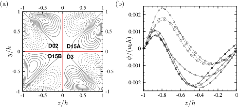
Figure 1: Panel (a), contours of the streamfunction $\psi$ in the range $-0.002\leq\psi/(u_{b}h)\leq 0.002$, in intervals of $0.0025$ (dashed lines denote negative values). Data are reported for flow cases D02 (top left), D15A (top right), D15B (bottom left), D3 (bottom right). Panel (b), 1D profiles at $y/h=-0.75$ (solid) and $y/h=-0.5$ (dashed) for case D02 (deltas), D15A (circles), D15B (diamond), D3 (squares).

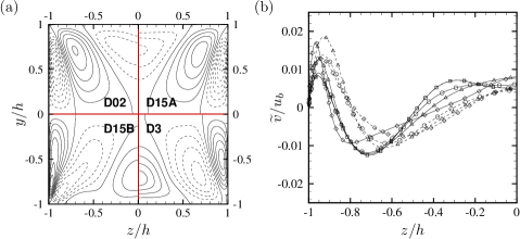
Figure 2: Panel (a), contours of the mean cross-stream velocity component $\widetilde{v}$ in the range $-0.02\leq\widetilde{v}/u_{b}\leq 0.02$, in intervals of $0.0025$ (dashed lines denote negative values). Data are reported for flow cases D02 (top left), D15A (top right), D15B (bottom left), D3 (bottom right). Panel (b), 1D profiles at $y/h=-0.75$ (solid) and $y/h=-0.5$ (dashed) for case D02 (deltas), D15A (circles), D15B (diamond), D3 (squares).

In this section we analyze the structure of the mean velocity field including the secondary motions, with special reference to establishing the effect of compressibility on the validity of compressibility transformations for the wall law. The structure of the secondary motions is hereafter analyzed by introducing a cross-flow stream function $\psi$, defined such that at any point over the duct cross section

$$-\overline{\rho}\widetilde{v}=\overline{\rho}_{w}\frac{\partial{\psi}}{\partial z},\quad\overline{\rho}\widetilde{w}=\overline{\rho}_{w}\frac{\partial{\psi}}{\partial y},$$ (8)

which satisfies mass conservation in the cross-stream plane. In figure 1 we show $\psi$ in a quarter of the duct, scaled with respect to $u_{b}$ and $h$, for the various flow cases of table 1. All the flow cases exhibit the same typical flow topology with eight counter-rotating eddies, which act to feed the low-momentum regions created at the corners. Figure 2 further shows that the cross-stream velocity component is characterized by a three-lobe structure, as in the incompressible case [21]. The cross-stream velocity peaks are found to scale reasonably well with the bulk flow velocity, regardless of Mach and Reynolds number, with maximum value of about $2\%$ of $u_{b}$, which is similar to the incompressible case [21].

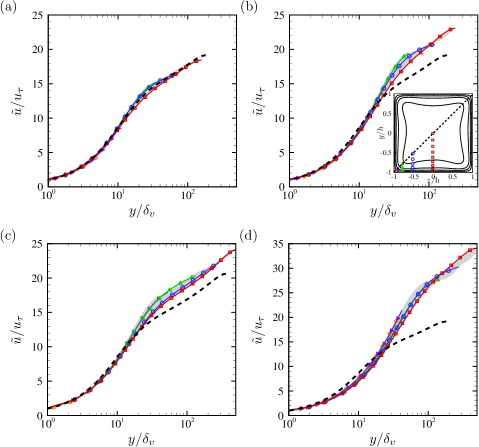
Figure 3: Mean streamwise velocity profiles along the $y$ direction (up to the corner bisector), given in local wall units at all $z$, for flow case D02 (a), D15A (b) D15B (c) and D3 (d). Representative stations along the bottom wall are highlighted, namely $z^{*}=15$ (diamonds), $(z+h)/h=0.1$ (right triangles), $(z+h)/h=0.25$ (triangles), $(z+h)/h=0.5$ (circles), $(z+h)/h=1$ (squares). The dashed lines denote mean profiles from DNS of pipe flow at $\mbox{{Re}}_{\tau}=180$ (a-b-d) and $\mbox{{Re}}_{\tau}=360$ (c) from [5], The inset panel (b) shows the mean streamwise velocity in the cross-stream plane with symbols denoting representative sections.

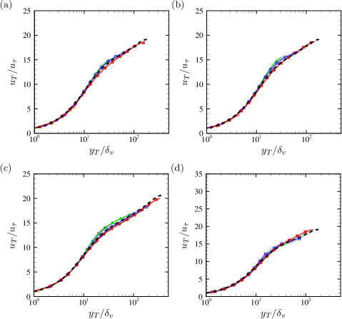
Figure 4: Mean streamwise velocity profiles transformed according to equation (9) along the $y$ direction (up to the corner bisector), given in local wall units at all $z$, for flow case D02 (${\mbox{{Re}}_{\tau}}_{T}^{*}=146$, panel a), D15A (${\mbox{{Re}}_{\tau}}_{T}^{*}=141$, panel b) D15B (${\mbox{{Re}}_{\tau}}_{T}^{*}=332$, panel c) and D3 (${\mbox{{Re}}_{\tau}}_{T}^{*}=145$, panel d). Representative stations along the bottom wall are highlighted, namely $z^{*}=15$ (diamonds), $(z+h)/h=0.1$ (right triangles), $(z+h)/h=0.25$ (triangles), $(z+h)/h=0.5$ (circles), $(z+h)/h=1$ (squares). The dashed lines denote mean profiles from DNS of pipe flow at $\mbox{{Re}}_{\tau}=180$ (a,b,d) and $\mbox{{Re}}_{\tau}=360$ (c) [5].

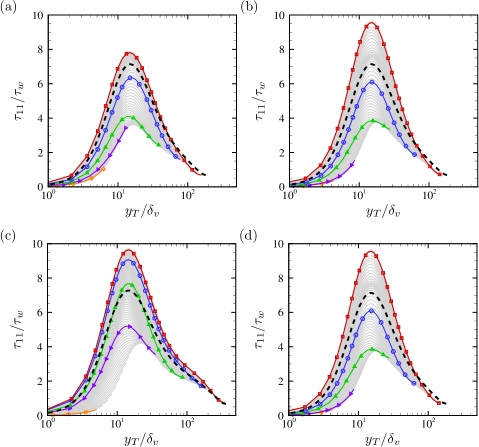
Figure 5: Streamwise turbulent stresses along the $y$ direction (up to the corner bisector), given in local wall units at all $z$, for flow case D02 (${\mbox{{Re}}_{\tau}}_{T}^{*}=146$, panel a), D15A (${\mbox{{Re}}_{\tau}}_{T}^{*}=141$, panel b) D15B (${\mbox{{Re}}_{\tau}}_{T}^{*}=332$, panel c) and D3 (${\mbox{{Re}}_{\tau}}_{T}^{*}=145$, panel d). Representative stations along the bottom wall are highlighted, namely $z^{*}=15$ (diamonds), $(z+h)/h=0.1$ (right triangles), $(z+h)/h=0.25$ (triangles), $(z+h)/h=0.5$ (circles), $(z+h)/h=1$ (squares). The dashed lines denote stress profiles from DNS of pipe flow at $\mbox{{Re}}_{\tau}=180$ (a,b,d) and $\mbox{{Re}}_{\tau}=360$ (c) [5].

The mean streamwise velocity field in compressible flows is generally characterized reverting to the concept of compressibility transformations. Morkovin [17] first postulated that if density fluctuations are negligible with respect to mean density variations, the direct effect of compressibility on turbulence reduces to variations of the mean thermodynamic properties. This led to the well known van Driest transformation [25], which is quite accurate for adiabatic walls, whereas it is known to fail for isothermal walls [14]. For the latter wall conditions, Trettel and Larsson [24] have recently derived a compressibility transformation for channel flow which relies on mean momentum balance and log-law universality. Pirozzoli et al. [21] showed that in incompressible square duct flow the streamwise velocity field is mainly influenced by the nearest wall, thus the wall law applies with reasonable accuracy up to the corner bisector. Based on this result and on the fact that the secondary motions are not affected by compressibility, we then introduce the TL transformation for $y$ (the direction normal to the nearest wall) and $u$,

$$y_{T}(y,z)=\int_{0}^{y}f_{T}(\eta,z)\,{\mathrm{d}}\eta,\quad u_{T}(y,z)=\int_{0}^{y}g_{T}(\eta,z)\,\frac{\partial\tilde{u}}{\partial\eta}(\eta,z){\mathrm{d}}\eta,$$ (9)

where the stretching functions are defined as

$$f_{T}(y,z)=\frac{\partial}{\partial y}\left(\frac{y}{R^{1/2}N}\right),\quad g_{T}(y,z)=RN\frac{\partial}{\partial y}\left(\frac{y}{R^{1/2}N}\right),$$ (10)

with $N(y,z)=\overline{\nu}/\overline{\nu}_{w}$, and $R(y,z)=\overline{\rho}/\overline{\rho}_{w}$. It is important to note that the stretching functions $f_{T}$ and $g_{T}$ depend both on $y$ and $z$ (through the mean density and mean viscosity), and likewise $y_{T}$ and $u_{T}$.

Figure 3 shows the mean velocity profiles as a function of the wall-normal distance up to the corner bisector (where mean velocity attains a maximum), in local wall units. For reference purposes, the mean velocity profiles from DNS of incompressible pipe flow are also reported [5]. Excellent collapse of the velocity profiles at various $z$ is recovered, also including the near-corner region. However, large differences are found among the different flow cases, especially at higher Mach number. The TL transformed velocity profiles are shown in figure 4, which now shows collapse of the velocity distributions both with respect to $z$ and across different flow cases. This confirms on one hand that the TL transformation derived for plane channel flow also holds with good approximation for square ducts. On the other hand, the figure also suggests that close similarity with the velocity distributions in incompressible pipe flow is recovered for matching values of an equivalent friction Reynolds number, which we define as

$${\mbox{{Re}}_{\tau}}_{T}^{*}=y_{T}^{*}(h)/\delta_{v}^{*}.$$ (11)

where

$$y_{T}^{*}(y)=\frac{1}{h}\int_{0}^{h}y_{T}(y,z)\mathrm{d}z,$$ (12)

is a stretched wall-normal coordinate averaged along the $z$ direction, which accounts in the mean for the variation of the local transformed scale $y_{T}$ with $z$. As in the incompressible case therefore, duct flow shows close similarity with pipe flow, which is a direct consequence of the fact that the intensity of the secondary flows is rather small [21].

The streamwise turbulent stress ($\tau_{11}$) normalized by the local wall shear stress is shown in figure 5, and compared with incompressible pipe flow data. Along most of the wall, the behaviour is qualitatively similar to canonical pipe flow, with a near-wall peak at $y^{+}\approx 12$. The scatter among the various $z$ sections appears to be generally much larger than for the mean velocity field, although it seems to become confined to the corner vicinity at high enough Re. The streamwise turbulent stress component exhibits a higher peak in the buffer layer at supersonic Mach number, which is not accurately captured by normalization with the local wall shear stress. This effect was observed in previous studies of canonical compressible flows [2, 9, 14], but no convincing explanation has been provided to date. Good collapse with incompressible pipe flow is by the way observed for all cases in the outer part of the wall layer.

3.2 Temperature field

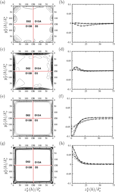
Figure 6: Contours (panels a, c, e, g), and profiles (panels b, d, f, h) of mean enthalpy budget terms (equation (13)) in global stretched inner units. Contours are shown in the range $-0.025\leq(.)/(\rho_{w}^{*}u_{\tau}^{*}T_{\tau}^{*}/\delta_{v}^{*})\leq 0.025$, in intervals of $3\cdot 10^{-3}$, dashed lines denoting negative values. From top to bottom we show convection, turbulent transport, viscous diffusion, and viscous dissipation. The 1D profiles are reported at $y^{*}=25$ (dashed lines) and $y^{*}=75$ (solid lines), for all cases (D02, triangles; D15A, circles; D15B, diamonds; D3, squares).

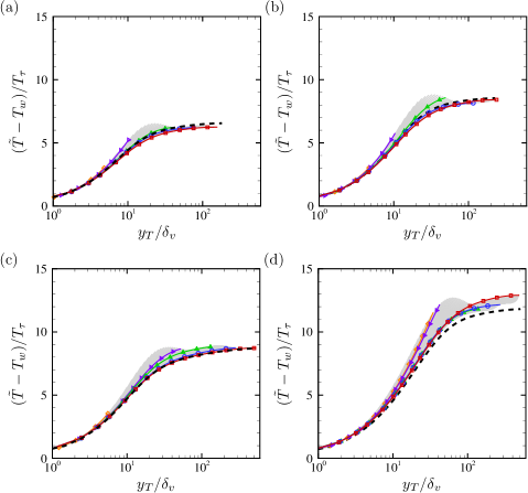
Figure 7: Mean temperature profiles along the $y$ direction (up to the corner bisector), given in local wall units at all $z$, for flow case D02 (${\mbox{{Re}}_{\tau}}_{T}^{*}=146$, panel a), D15A (${\mbox{{Re}}_{\tau}}_{T}^{*}=141$, panel b) D15B (${\mbox{{Re}}_{\tau}}_{T}^{*}=332$, panel c) and D3 (${\mbox{{Re}}_{\tau}}_{T}^{*}=145$, panel d). Representative stations along the bottom wall are highlighted, namely $z^{*}=15$ (diamonds), $(z+h)/h=0.1$ (right triangles), $(z+h)/h=0.25$ (triangles), $(z+h)/h=0.5$ (circles), $(z+h)/h=1$ (squares). The dashed lines denote mean profiles from DNS of pipe flow at $\mbox{{Re}}_{\tau}=143$ (a,b,d) and $\mbox{{Re}}_{\tau}=334$ (c) [13]. The inset in panel (b) shows the mean streamwise velocity in the cross-stream plane with symbols denoting representative $z$ stations.

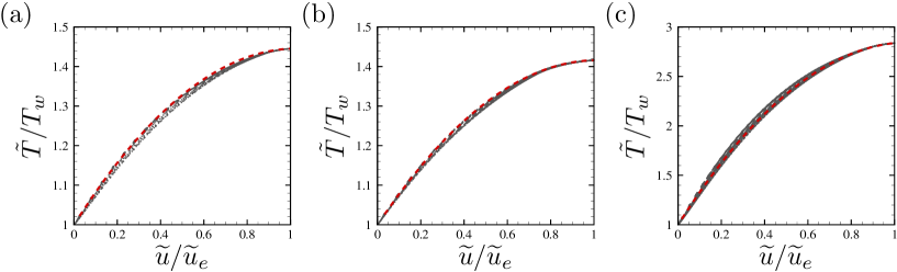
Figure 8: Scatter plots of mean temperature versus mean velocity for all points in the duct cross section for flow cases D15A (a), D15B (b), D3 (c). The subscript $e$ refers to duct centerline values. The dashed line denotes the generalized temperature/velocity relation given in equation (14).

The temperature field is herein analyzed starting from the averaged enthalpy transport equation,

$$\begin{split}\underbrace{\frac{\partial\overline{\rho}c_{p}\widetilde{v}\widetilde{T}}{\partial y}+\frac{\partial\overline{\rho}c_{p}\widetilde{w}\widetilde{T}}{\partial z}}_{C}&=\underbrace{\frac{\partial}{\partial y}\left(\overline{k}\frac{\partial\widetilde{T}}{\partial y}\right)+\frac{\partial}{\partial z}\left(\overline{k}\frac{\partial\widetilde{T}}{\partial z}\right)}_{D}+\\ &\underbrace{+\overline{u\frac{\partial p}{\partial x}}+\overline{v\frac{\partial p}{\partial y}}+\overline{w\frac{\partial p}{\partial z}}}_{P}+\underbrace{\overline{\sigma_{ij}\frac{\partial u_{i}}{\partial x_{j}}}}_{\Psi}\underbrace{-\frac{\partial\overline{\rho}c_{p}\widetilde{v^{\prime\prime}T^{\prime\prime}}}{\partial y}-\frac{\partial\overline{\rho}c_{p}\widetilde{w^{\prime\prime}T^{\prime\prime}}}{\partial z}}_{T},\end{split}$$ (13)

where the terms $C$, $D$, $P$, $\Psi$, and $T$ represent convection, viscous diffusion, pressure work, viscous dissipation and turbulent transport. The various contributions to the budget are reported in figure 6, in global stretched inner units, upon normalization of temperature with respect to the global friction temperature, both in the cross-stream plane and at selected wall-normal sections. The pressure work term is not reported, being negligible in all cases. The figure shows that inner scaling yields good collapse across different Mach (cases D02, D15A, D3) and Reynolds numbers (D15A, D15B). Similar to what found from the mean momentum balance equation in the incompressible case [21], we note that mean convection is mainly relevant at the duct corners, whereas it plays a minor role with respect to the other terms in the bulk region. Viscous diffusion and dissipation contribute most to the budget, and they are partially balanced by turbulent heat transport in the buffer layer.

Figure 7 shows the inner-scaled wall-normal temperature profiles up to the corner bisector, and it supports good universality in the spanwise direction, and good agreement between duct flow and supersonic pipe flow data at matching Mach and Reynolds number [13]. Nevertheless, temperature does not exhibit any logarithmic layer nor universality with respect to Reynolds and Mach number, unlike previously observed for the mean velocity field (see figure 4). Corner effects also seem to be more significant than for the mean velocity, yielding earlier deviation from a common distribution when approaching the wall. This behavior may be explained by noting that in the current case of isothermal wall the energy balance is mainly controlled by aerodynamic heating, which is associated with viscous dissipation, and which acts as a non-uniform spatial forcing. As shown in the forthcoming Section, in the case of a passive scalar with spatially uniform forcing a logarithmic layer does in fact emerge as for the mean velocity. Hence, deviations of the temperature distributions from a logarithmic behavior are the likely consequence of non-uniform heating, and regarding the temperature as a passive scalar may lead to incorrect conclusions, even at low Mach numbers.

Knowledge of the temperature distribution in compressible flow is necessary for the prediction of friction [23]. In particular, based on the distribution of $T$ one can derive the mean velocity distribution through reverse application of the compressibility transformation introduced in Section 3.1, and temperature/velocity relationships are needed for the purpose. The classical temperature/velocity relation by Walz [28] has proven its accuracy in the case of adiabatic walls [4], whereas it is found to fail in the case of isothermal walls [14]. Recently, Zhang et al. [29] derived the following generalized temperature/velocity relation,

$$\frac{\widetilde{T}}{T_{w}}=1+\frac{T_{rg}-T_{w}}{T_{w}}\frac{\widetilde{u}}{\widetilde{u}_{e}}+\frac{\widetilde{T}_{e}-T_{rg}}{T_{w}}\left(\frac{\widetilde{u}}{\widetilde{u}_{e}}\right)^{2},$$ (14)

where $T_{rg}=\tilde{T}_{e}+r_{g}\tilde{u}_{e}^{2}/(2c_{p})$ is a generalized recovery temperature, $r_{g}=2c_{p}(T_{w}-\tilde{T}_{e})/\tilde{u}_{e}^{2}-2\mbox{{Pr}}q_{w}/(\tilde{u}_{e}\tau_{w})$ is a generalized recovery factor, and $u_{e}$ and $T_{e}$ are the external values of velocity and temperature, here interpreted as the duct centerline values. Equation (14) explicitly takes into account the wall heat flux $q_{w}$, and it reduces to Walz relation in the case of adiabatic walls. Figure 8 shows scatter plots of temperature as a function of velocity for all points in the duct cross section. Nearly perfect collapse of the supersonic DNS data with the predictions of equation (14) is observed, hence from integration of equation (10) one can reconstruct the full velocity field for assigned values of the bulk Reynolds and Mach numbers.

3.3 Passive scalar field

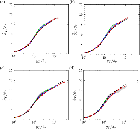
Figure 9: Mean TL-transformed passive scalar profiles along the $y$ direction (up to the corner bisector), given in local wall units at all $z$, for flow case D02 (${\mbox{{Re}}_{\tau}}_{T}^{*}=146$, panel a), D15A (${\mbox{{Re}}_{\tau}}_{T}^{*}=141$, panel b) D15B (${\mbox{{Re}}_{\tau}}_{T}^{*}=332$, panel c) and D3 (${\mbox{{Re}}_{\tau}}_{T}^{*}=145$, panel d). $\phi_{\tau}$ is the friction value of the passive scalar, defined in equation (6). Representative stations along the bottom wall are highlighted, namely $z^{*}=15$ (diamonds), $(z+h)/h=0.1$ (right triangles), $(z+h)/h=0.25$ (triangles), $(z+h)/h=0.5$ (circles), $(z+h)/h=1$ (squares). The dashed lines denote fits of experimental incompressible pipe flow data by Kader [10]. Different panels show flow cases D02 (a), D15A (b), D15B (c), D3 (d).

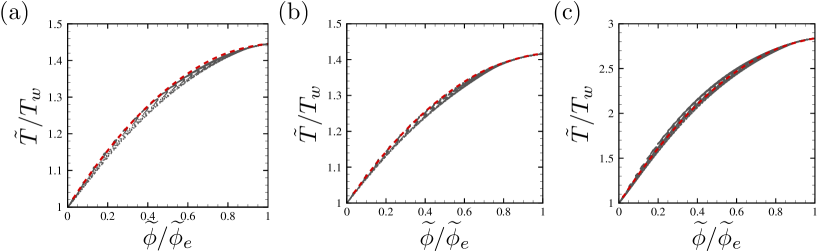
Figure 10: Scatter plots of mean temperature versus mean passive scalar for all points in the duct cross section for flow cases D15A (a), D15B (b), D3 (c). The subscript $e$ refers to duct centerline values. The dashed line denotes the generalized temperature/passive scalar relation given in equation (16).

In this section we study the transport of a passive scalar field as from equation (1d) at unit Schmidt number, previously studied in channel flows in the incompressible case [20], and for supersonic Mach number [6]. Exploiting the similarity between the governing equation of a passive scalar (equation (1d)) and the streamwise momentum equation (equation (1b)), we introduce a transformation for the mean scalar field which mimics the TL transformation (equation (9)), as follows

$$\phi_{T}(y,z)=\int_{0}^{y}g_{T}(\eta,z)\,\frac{\partial\tilde{\phi}}{\partial\eta}(\eta,z)\,{\mathrm{d}}\eta,$$ (15)

with $g_{T}$ given in equation (10). Figure 9 shows the inner-scaled transformed passive scalar profiles, compared with the correlations developed by Kader [10] for incompressible pipe flow, which include an inertial layer with logarithmic dependence on the wall distance. The figure does in fact show accurate collapse of the $\phi_{T}$ distributions with respect to $z$ across the different flow cases and with the incompressible fittings. This findings supports our conjecture that the TL transformation can be extended to predict the behavior of passive scalars in compressible flow. Again based on the close similarity between $\phi$ and $u$, we consider a generalization of equation (14) to relate temperature and passive scalars, namely

$$\frac{\tilde{T}}{T_{w}}=1+\frac{T_{rg}-T_{w}}{T_{w}}\frac{\widetilde{\phi}}{\widetilde{\phi}_{e}}+\frac{\widetilde{T}_{e}-T_{rg}}{T_{w}}\left(\frac{\widetilde{\phi}}{\widetilde{\phi}_{e}}\right)^{2},$$ (16)

where $\widetilde{\phi}_{e}$ denotes the mean value of the passive scalar at the duct centerline. Figure 10 shows the scatter plots of temperature as a function of the mean passive scalar for all points in the duct cross section. As for the velocity field, near perfect collapse of the supersonic DNS data with the predictions of equation 16 is observed, which leads us to conclude that from integration of equation (15) one can reconstruct the full passive scalar field for assigned values of the bulk Reynolds and Mach numbers.

4 Conclusions

We have carried out DNS of compressible square duct flow at various Mach and Reynolds numbers, with the aim of clarifying the behavior of the mean velocity, temperature and passive scalar fields. All the flow cases exhibit the same typical secondary flow structure including eight counter-rotating eddies, which act to supply momentum to the duct corners. The cross-stream velocity peaks are found to scale reasonably well with the bulk flow velocity, regardless of Mach and Reynolds number, with maximum value of about $2\%u_{b}$, which is also consistent with the incompressible case [21]. The analysis of the mean streamwise velocity field leads to conclude that the TL compressibility transformation derived for planar channel flow [24] can be extended to square ducts, upon local application in the direction normal to the nearest wall. The DNS data further suggest close similarity of the transformed velocity distributions with those in incompressible pipe flow at matching values of an equivalent friction Reynolds number, defined in equation (11).

Regarding the temperature field, we find that the various contributions to the enthalpy budget scale well when expressed in inner units, irrespective of the Mach and Reynolds numbers. Similar to the incompressible case, we find that mean convection is mainly relevant at the duct corners, whereas it plays a minor role with respect to the other terms in the bulk region. Viscous diffusion and dissipation contribute most to the budget, and they are partially balanced by turbulent heat transport in the buffer layer. The energy balance is mainly controlled by aerodynamic heating, which acts as a non-uniform spatial forcing, and consequently the mean temperature does not exhibit any logarithmic layer nor universality with respect to Reynolds and Mach number.

Exploiting the similarity between the governing equation of a passive scalar and the streamwise momentum equation, we show that the TL transformation can also be extended to predict the behavior of passive scalars in compressible flow, for which a logarithmic layer is found. We further show that a generalized form of Waltz’ equation can be used to relate the mean velocity and passive scalar fields with the mean temperature field. These results together point to a relatively simple representation of the mean flow properties in compressible duct flow, which can be exploited to obtain predictive formulas for friction and heat transfer for assigned values of the bulk Reynolds and Mach numbers.

Acknowledgements
We acknowledge that most of the results reported in this paper have been achieved using the PRACE Research Infrastructure resource MARCONI based at CINECA, Casalecchio di Reno, Italy.

References

- Bradshaw [1987] P. Bradshaw. Turbulent secondary flows. Annu. Rev. Fluid Mech., 19(1):53–74, 1987.
- Coleman et al. [1995] G.N. Coleman, J. Kim, and R.D. Moser. A numerical study of turbulent supersonic isothermal-wall channel flow. J. Fluid Mech., 305:159–183, 1995.
- Davis et al. [1986] D.O. Davis, F.B. Gessner, and G.D. Kerlick. Experimental and numerical investigation of supersonic turbulent flow through a square duct. AIAA J., 24(9):1508–1515, 1986.
- Duan et al. [2010] L. Duan, I. Beekman, and M.P. Martin. Direct numerical simulation of hypersonic turbulent boundary layers. Part 2. Effect of wall temperature. J. Fluid Mech., 655:419–445, 2010.
- El Khoury et al. [2013] J.K. El Khoury, P. Schlatter, A. Noorani, P.F. Fischer, G. Brethouwer, and A.V. Johansson. Direct numerical simulation of turbulent pipe flow at moderately high Reynolds numbers. Flow Turbul. Combust., 91(3):475–495, 2013.
- Foysi and Friedrich [2005] H. Foysi and R. Friedrich. DNS of Passive Scalar Transport in Turbulent supersonic channel flow. In High Performance Computing in Science and Engineering, Munich 2004, pages 107–117. Springer, 2005.
- Gavrilakis [1992] S. Gavrilakis. Numerical simulation of low-Reynolds-number turbulent flow through a straight square duct. J. Fluid Mech., 244:101–129, 1992.
- Ghosh et al. [2008] S. Ghosh, J. Sesterhenn, and R. Friedrich. Large-eddy simulation of supersonic turbulent flow in axisymmetric nozzles and diffusers. Int. J. Heat Fluid Flow, 29(3):579–590, 2008.
- Ghosh et al. [2010] S. Ghosh, H. Foysi, and R. Friedrich. Compressible turbulent channel and pipe flow: similarities and differences. J. Fluid Mech., 648:155–181, 2010.
- Kader [1981] B.A. Kader. Temperature and concentration profiles in fully turbulent boundary layers. Int. J. Heat Mass Transf., 24(9):1541–1544, 1981.
- Klein et al. [2003] M. Klein, A. Sadiki, and J. Janicka. A digital filter based generation of inflow data for spatially developing direct numerical or large eddy simulations. J. Comput. Phys., 186(2):652–665, 2003.
- Mani et al. [2013] M. Mani, D.A. Babcock, C.M. Winkler, and P.R. Spalart. Predictions of a supersonic turbulent flow in a square duct. AIAA Paper, 860:2013, 2013.
- Modesti [2017] D. Modesti. Direct numerical simulation of internal compressible flows at high Reynolds number: numerical and physical insight. PhD thesis, La Sapienza Unversità di Roma, 2017. Published online: http://hdl.handle.net/11573/939526.
- Modesti and Pirozzoli [2016] D. Modesti and S. Pirozzoli. Reynolds and Mach number effects in compressible turbulent channel flow. Int. J. Heat Fluid Flow, 59:33–49, 2016.
- Modesti and Pirozzoli [2018] D. Modesti and S. Pirozzoli. An efficient semi-implicit solver for direct numerical simulation of compressible flows at all speeds. J. Sci. Comput., 75(1):308–331, 2018.
- Morajkar and Gamba [2016] R.R. Morajkar and M. Gamba. Turbulence characteristics of supersonic corner flows in a low aspect ratio rectangular channel. In 54th AIAA Aerospace Sciences Meeting, page 1590, 2016.
- Morkovin [1962] M.V. Morkovin. Effects of compressibility on turbulent flows. In Mécanique de la Turbulence, pages 367–380. A. Favre, 1962.
- Nikuradse [1926] J. Nikuradse. Untersuchung über die Geschwindigkeitsverteilung in turbulenten Strömungen. Vdi-verlag, 1926.
- Pirozzoli [2010] S. Pirozzoli. Generalized conservative approximations of split convective derivative operators. J. Comput Phys., 229(19):7180–7190, 2010.
- Pirozzoli et al. [2016] S. Pirozzoli, M. Bernardini, and P. Orlandi. Passive scalars in turbulent channel flow at high Reynolds number. J. Fluid Mech., 788:614–639, 2016.
- Pirozzoli et al. [2018] S. Pirozzoli, D. Modesti, P. Orlandi, and F. Grasso. Turbulence and secondary motions in square duct flow. J. Fluid Mech., 840:631–655, 2018.
- Prandtl [1927] L. Prandtl. Über den reibungswiderstand strömender luft. Reports of the Aerod. Versuchsanst, Göttingen, Germany, 3rd Series, 1927.
- Smits and Dussauge [2006] A.J. Smits and J.-P. Dussauge. Turbulent Shear Layers in Supersonic Flow. 2nd edn., American Institute of Physics, New York, 2006.
- Trettel and Larsson [2016] A. Trettel and J. Larsson. Mean velocity scaling for compressible wall turbulence with heat transfer. Phys. Fluids (1994-present), 28(2):026102, 2016.
- van Driest [1951] E.R. van Driest. Turbulent boundary layer in compressible fluids. J. Aero. Sci., 18:145–160, 1951.
- Vane and Lele [2015] Z.P. Vane and S.K. Lele. Prediction of Turbulent Secondary Flows in Ducts Using Equilibrium Wall-Modeled LES. In 53rd AIAA Aerospace Sciences Meeting, page 1274, 2015.
- Vázquez and Métais [2002] M.S. Vázquez and O. Métais. Large-eddy simulation of the turbulent flow through a heated square duct. J. Fluid Mech., 453:201–238, 2002.
- Walz [1959] A. Walz. Compressible turbulent boundary layers with heat transfer and pressure gradient in flow direction. J. Res. Natl. Bur. Stand., 63, 1959.
- Zhang et al. [2014] Y.S. Zhang, W.T. Bi, F. Hussain, and Z.S. She. A generalized Reynolds analogy for compressible wall-bounded turbulent flows. J. Fluid Mech., 739:392–420, 2014.