Generalized Langevin dynamics: Construction and numerical integration of non-Markovian particle-based models

Abstract

We propose a Generalized Langevin dynamics (GLD) technique to construct non-Markovian particle-based coarse-grained models from fine-grained reference simulations and to efficiently integrate them. The proposed GLD model has the form of a discretized generalized Langevin equation with distance-dependent two-particle contributions to the self- and pair-memory kernels. The memory kernels are iteratively reconstructed from the dynamical correlation functions of an underlying fine-grained system. We develop a simulation algorithm for this class of non-Markovian models that scales linearly with the number of coarse-grained particles. Our GLD method is suitable for coarse-grained studies of systems with incomplete time scale separation, as is often encountered, e.g., in soft matter systems.

We apply the method to a suspension of nanocolloids with frequency-dependent hydrodynamic interactions. We show that the results from GLD simulations perfectly reproduce the dynamics of the underlying fine-grained system. The effective speedup of these simulations amounts to a factor of about $10^{4}$. Additionally, the transferability of the coarse-grained model with respect to changes of the nanocolloid density is investigated. The results indicate that the model is transferable to systems with nanocolloid densities that differ by up to one order of magnitude from the density of the reference system.

I Introduction

Many materials, in particular soft matter, exhibit dynamics on multiple length and time scales. Examples are protein folding Frembgen-Kesner and Elcock (2009), polymer aggregation Tomilov et al. (2013) or colloidal crystallization Palberg (1999); Vermant and Solomon (2005). Since these problems are difficult to access with standard atomistic simulations, one typically considers coarse-grained (CG) models with fewer degrees of freedom. A vast variety of different coarse-graining techniques have been suggested that reduce the dimensionality of a system Ermak (1975); van Gunsteren and Berendsen (1982); Lyubartsev and Laaksonen (1995); Reith et al. (2003); Izvekov et al. (2004); Shell (2008); Hijón et al. (2010). Most of these methods either do not target the dynamical properties of the fine-grained system at all, or they assume complete time scale separation: They postulate that the dynamics of the relevant, coarse-grained particles is much slower than the relaxation time of the irrelevant, neglected degrees of freedom, and thus take the CG dynamics to be Markovian. In real systems, however, the relevant time scales often overlap and the Markovian assumption is not justified. In such cases, a more appropriate framework for the construction of dynamic coarse-grained models is the (multidimensional) generalized Langevin equation (GLE) Kinjo and Hyodo (2007)

$$M\dot{\bm{V}}_{i}(t)=\bm{F}_{i}^{\text{C}}(t)-\int_{0}^{t}\!\!\!\!\text{d}s\>\sum_{j}\bm{K}_{ij}(t,s)\bm{V}_{j}(s)+\partial\bm{F}_{i}(t),$$ (1)

where $\bm{V}_{i}(t)$ denotes the velocity of the CG particle $i$, $M$ its mass, $\bm{F}_{i}^{\text{C}}(t)$ the conservative forces, and $\partial\bm{F}_{i}(t)$ the fluctuating forces acting on it. The memory kernel tensor $\bm{K}_{ij}(t,s)$ determines the non-Markovian dissipative self- and pair-interactions of the CG particles. Note that both $\bm{F}_{i}^{\text{C}}$ and $\bm{K}_{ij}$ are functions of the positions $\bm{R}_{j}$ of all particles $j$. The fluctuating force is related to the memory kernel tensor via the fluctuation-dissipation theorem (FDT),

$$\left\langle\partial\bm{F}_{i}(t)\partial\bm{F}_{j}(t^{\prime})\right\rangle=k_{\text{B}}T\>\bm{K}_{ij}(t,t^{\prime}),$$ (2)

with the Boltzmann constant $k_{\text{B}}$ and the thermodynamic temperature $T$. The GLE thus describes a system of particles in a canonical ensemble with constant temperature $T$. The general form of the GLE results from the Mori-Zwanzig projection operator formalism, which was introduced roughly 50 years ago to theoretically understand the process of systematic coarse-graining Zwanzig (1961); Mori (1965); Zwanzig (2001). We note that the average $\left\langle\cdot\right\rangle$ in Eq. (2) is a conditional average for fixed CG configuration and thus depends on the position of all CG particles, just like the memory kernel.

In recent years, the GLE has become increasingly popular as a tool for mesoscopic modeling Smith and Harris (1990); Ceriotti et al. (2010); Córdoba et al. (2012); Baczewski and Bond (2013); Li et al. (2015); Davtyan et al. (2015); Li et al. (2017); Jung et al. (2017); Meyer et al. (2017). However, most studies so far were restricted to systems with one or two particles. One problem with GLE-modeling of many-particle systems is the high dimension of the memory tensor $\bm{K}_{ij}$, which complicates the generation of random forces with correct correlations (Eq. (2)). The problem can be avoided if one simply neglects cross-correlations in the friction kernel ($\bm{K}_{ij}=\delta_{ij}\bm{K}_{ii}$). An alternative Ansatz was recently proposed by Li et al. Li et al. (2015, 2017). These authors generalized the standard dissipative particle dynamics (DPD) equations of motion to a non-Markovian DPD (NM-DPD) method with frequency-dependent pair friction terms. In NM-DPD, the dissipative friction term in Eq. (1) is thus taken to have the form

$$\int_{0}^{t}\text{d}s\>\sum_{j}\bm{K}_{ij}^{\text{NM-DPD}}{(t,s)}\bm{V}_{j}(s)$$

$$=\int_{0}^{t}\text{d}s\>\sum_{j\neq i}\bm{K}_{ij}(t-s)\>(\bm{V}_{j}(s)-\bm{V}_{i}(s)).$$

As in standard DPD, the correlated random forces $\partial\bm{F}_{i}$ can then be written as sums of uncorrelated random pair forces $\partial\bm{F}_{ij}=-\partial\bm{F}_{ji}$, which greatly simplifies the problem of random force generation.

To the best of our knowledge, the method of Li et al. is the only method published so far that enables non-Markovian modeling with dissipative pair-interactions. They applied their formalism to star-polymer melts and reported promising results. However, the NM-DPD assumption (I) implies an additive relation $\bm{K}_{ii}^{\text{NM-DPD}}=-\sum_{j\neq i}\bm{K}_{ij}$ in Eq. (1), which is often not correct. Moreover, NM-DPD models are Galilean invariant by construction, which is clearly inappropriate if the CG model describes the motion of CG particles in a background medium – as is the case in implicit solvent models.

In the present paper we propose a more general approach, the ”generalized Langevin dynamics” (GLD) method. Like the above-mentioned models, it is also derived from the GLE, but it relies on weaker assumptions (the latter can in fact be considered as special cases of the GLD model). The method can be seen as a generalization of Brownian dynamics (BD) with frequency-dependent friction tensors Ermak (1975); van Gunsteren and Berendsen (1982). It can therefore be applied to polymers as well as colloidal systems with incomplete separation of time scales.

In a recent paper, we have investigated the dissipative pair-interactions in a system of two isolated nanocolloids by theory and molecular dynamics simulations Jung and Schmid (2017). Here, we consider suspensions of many nanocolloids. We construct a coarse-grained GLD model from simulation data for a fine-grained explicit solvent model at a reference nanocolloid density $\rho_{0}$. Then we perform GLD simulations at a set of densities $\rho$. This allows us to validate the method (by comparing the results of the GLD simulations at $\rho=\rho_{0}$ with those from the fine-grained simulations) and to investigate other properties such as the transferability and computational efficiency (benchmarks) of the GLD method.

Our paper is organized as follows: In Sec. II we introduce the Generalized Langevin dynamics method. We derive the discretized equations of motion and present a method how to efficiently determine the time- and cross-correlated fluctuating forces. In Sec. III we then generalize the iterative memory reconstruction (IMRV) method published in earlier work Jung et al. (2017) and demonstrate how it can be used to reconstruct memory kernels from atomistic simulations. Our results are presented and discussed in Sec. IV. We summarize and conclude in Sec. V.

II Generalized Langevin dynamics

II.1 Basic Model

In the following, we consider a system of $N$ coarse-grained identical particles with positions $\bm{R}_{i}(t)$ and velocities $\bm{V}_{i}(t)$ in three dimensions. Our only approximation is to neglect dissipative many-body interactions. The memory kernel in the generalized Langevin equation for particle $i$, Eq.  (1), can then be written as

$$\bm{K}_{ij}(t,s)=\left\{\begin{array}[]{lcr}\bm{K}^{\text{self}}{[\{\bm{R}_{ik}(t)\},t-s]}&:&i=j\\ \bm{K}^{\text{p}}{[\bm{R}_{ij}(t),t-s]}&:&i\neq j\end{array}\right.$$ (4)

with

$$\bm{K}^{\text{self}}{[\{\bm{R}_{ik}(t)\},\tau]}=\bm{K}^{\text{s}}(\tau)+\sum_{k\neq i}\Delta\bm{K}^{\text{s}}{[\bm{R}_{ik}(t),\tau]}$$ (5)

and $\bm{R}_{ij}(t)=\bm{R}_{i}(t)-\bm{R}_{j}(t)$. Here we have expressed the memory kernel tensor in terms of $3\times 3$ dimensional ”pair-memory” and ”self-memory” kernels ($\bm{K}^{\text{p}}$ and $\bm{K}^{\text{self}}$, respectively), and we have taken into account the possibility that nearby particles may affect the self-memory via the sum over $\Delta\bm{K}^{\text{s}}$. If the pair interactions are strong, it is important to include the latter contribution to the self-interactions, as has been shown in Ref. (25) and will also be apparent in Sec. III.

We expect that in many applications, the two-particle contributions to the memory kernels, $\bm{K}^{\text{p}}$ and $\Delta\bm{K}^{\text{s}}$, can be separated into contributions parallel and orthogonal to the line connecting the centers of the particles. If this is the case, the two-particle contributions to the memory kernels can be decomposed according to

$$\bm{K}^{\text{p}}{[\bm{R}_{ij}(t),t^{\prime}]} \approx {K}_{\parallel}^{\text{p}}[R_{ij}(t),t^{\prime}]\,\bm{{e}}_{ij}\bm{{e}}^{T}_{ij}$$

$$+{K}_{\perp}^{\text{p}}{[R_{ij}(t),t^{\prime}]}(1-\bm{{e}}_{ij}\bm{{e}}^{T}_{ij}),$$

$$\Delta\bm{K}^{\text{s}}{[\bm{R}_{ij}(t),t^{\prime}]} \approx \Delta{K}_{\parallel}^{\text{s}}[R_{ij}(t),t^{\prime}]\,\bm{{e}}_{ij}\bm{{e}}^{T}_{ij}$$

$$+\Delta{K}_{\perp}^{\text{s}}[R_{ij}(t),t^{\prime}](1-\bm{{e}}_{ij}\bm{{e}}^{T}_{ij}).$$

where $R_{ij}(t)=|\bm{R}_{ij}(t)|$ and $\bm{{e}}_{ij}=\bm{R}_{ij}(t)/R_{ij}(t)$. In our numerical studies (Secs. III and IV), we will only consider the parallel components of $\bm{K}^{\text{p}}$ and $\Delta\bm{K}^{\text{s}}$ for simplicity. This approximation is justified by the theoretical and simulation results in Ref. (25). Additionally, we will assume that the single-particle memory kernel is isotropic, $\bm{K}^{\text{s}}(\tau)={K}^{\text{s}}(\tau)\bm{1}$, as it should be, given the symmetry of our system.

II.2 Discretized Model Equations

Having defined the basic model, Eq. (1) with (4) and (5), our next task is to construct a numerical integrator. To this end, we first introduce discretized memory kernels $\bm{K}_{m}$, defined as

$$\bm{K}(t-s)=\sum_{m=0}^{m_{\text{max}}-1}\bm{K}_{m}\delta(t-m\Delta t_{\text{}})$$ (8)

with the time step $\Delta t_{\text{}}$. The cutoff $m_{\text{max}}$ determines the longest time scale $\tau_{\text{mem}}=m_{\text{max}}\Delta t_{\text{}}$ on which memory effects are considered in the model. Introducing such a cutoff is necessary for numerical reasons. It must be optimized such that the GLD model is still computationally efficient while capturing the relevant memory effects in the underlying microscopic model. In some cases, the discretization and cutoff of the memory kernel can be circumvented by introducing auxiliary variable expansions Ceriotti et al. (2010); Córdoba et al. (2012, 2012); Baczewski and Bond (2013); Li et al. (2017). Here, the idea is to replace the non-Markovian equations of motion by Markovian equations for a system with virtual additional degrees of freedom. The additional, auxiliary variables then introduce memory effects in the dynamics of the ”real” particles, and they can be constructed in a systematic manner by fitting the target memory kernel to a sum of (complex) exponentials (see Appendix C). For the systems considered in the present work, it was, however, not possible to utilize this expansion – mainly due to problems with the distance-dependent two-particle contributions to the memory, $\Delta\bm{K}^{\text{s}}$ and $\bm{K}^{\text{p}}$. This is discussed in more detail in Appendix C.

Inserting the discrete version of the memory kernels, Eq. (8), the GLD equation (1) with (4) and (5) take the form

$$M\dot{\bm{V}}_{i}(t) = \bm{F}_{i}^{\text{C}}[\{\bm{R}_{j}(t)\}]$$

$$- \sum_{m=0}^{m_{\text{max}}-1}\bigg{\{}\sum_{j\neq i}\bm{K}_{m}^{\text{p}}[\bm{R}_{ij}(t)]\>\bm{V}_{j}(t-m\Delta t_{\text{}})$$

$$\quad+\>\bm{K}_{m}^{\text{self}}[\{\bm{R}_{ik}(t)\}]\>\bm{V}_{i}(t-m\Delta t_{\text{}})\bigg{\}}+\partial\bm{F}_{i}(t)$$

with the fluctuation-dissipation relation

$$\langle\partial\bm{F}_{i}(t)\partial\bm{F}_{j}(t^{\prime})\rangle=k_{\text{B}}T\!\!\sum_{m=0}^{m_{\text{max}}-1}\!\!a_{m}\delta(t-t^{\prime}-m\Delta t_{\text{}})$$

$$\times\Big{(}\delta_{ij}\bm{K}_{m}^{\text{self}}[\{\bm{R}_{ik}(t)\}]+(1-\delta_{ij})\bm{K}_{m}^{\text{p}}[\bm{R}_{ij}(t)]\Big{)},$$

where $\bm{K}_{m}^{\text{self}}[\{\bm{R}_{ik}\}]=\bm{K}_{m}^{\text{s}}+\sum_{k\neq i}\Delta\bm{K}_{m}^{\text{s}}[\bm{R}_{ik}(t)]$ and the prefactors $a_{m}$ are given by $a_{0}=2$ and $a_{m}=1$ for $m\neq 0$. The derivation of these equations follows closely that of Eqs. (12)-(17) in Ref. (23) and will not be repeated here.

Starting from Eqs. (II.2)-(II.2), we can derive a numerical integrator for the GLE following a scheme proposed by Grønbech-Jensen and Farago Grønbech-Jensen and Farago (2013). In earlier work Jung et al. (2017), we have applied this scheme to construct an integrator for the single-particle GLE; here, we extend that work to multiparticle GLD with two-particle contributions to the memory kernel. The derivation of the algorithm is presented in Appendix A. The final equations read

$$\bm{R}_{i,n+1} = \bm{R}_{i,n}+\Delta t_{\text{}}\>\bm{a}\>\bm{V}_{i,n}$$

$$+\frac{\Delta t_{\text{}}^{2}}{2M}\>\bm{b}\>(\bm{F}_{i,n}^{\text{C}}+{\bm{F}_{i,n}^{\text{D}}}^{\prime}+\bm{F}_{i,n}^{\text{R}})$$

$$\bm{V}_{i,n+1} = \bm{a}\>\bm{V}_{i,n}+\frac{\Delta t_{\text{}}}{2M}\>(\bm{a}\>\bm{F}_{i,n}^{\text{C}}+\bm{F}_{i,n+1}^{\text{C}})$$

$$+\frac{\Delta t_{\text{}}}{M}\>\bm{b}\>({\bm{F}_{i,n}^{\text{D}}}^{\prime}+\bm{F}_{i,n}^{\text{R}})$$

where we have introduced the shortcut notations $\bm{R}_{i,n}=\bm{R}_{i}(n\Delta t_{\text{}})$, $\bm{V}_{i,n}=\bm{V}_{i}(n\Delta t_{\text{}})$, $\bm{F}_{i,n}^{\text{C}}=\bm{F}_{i}^{\text{C}}[\{\bm{R}_{j,n}\}]$, and defined the matrices

$$\bm{b}=\Big{[}\bm{1}+\frac{\Delta t_{\text{}}}{2M}\bm{K}_{0}^{\text{s}}\Big{]}^{-1},\quad\bm{a}=\bm{b}\>\Big{[}\bm{1}-\frac{\Delta t_{\text{}}}{2M}\bm{K}_{0}^{\text{s}}\Big{]},$$ (13)

as well as the dissipative force vector

$${\bm{F}_{i,n}^{\text{D}}}^{\prime} = -\sum_{j\neq i}\big{(}\bm{K}_{0}^{\text{p}}[\bm{R}_{ij,n}]\>\bm{V}_{j,n}+\Delta\bm{K}_{0}^{\text{s}}[\bm{R}_{ij,n}]\>\bm{V}_{i,n}\big{)}$$

$$-\frac{1}{\Delta t_{\text{}}}\!\!\!\sum_{m=1}^{m_{\text{max}}-1}\bigg{\{}\sum_{j\neq i}\bm{K}_{m}^{\text{p}}[\bm{R}_{ij,n}]\,\Delta\bm{R}_{j,n-m}$$

$$\qquad\qquad+\>\Big{(}\bm{K}_{m}^{\text{s}}+\sum_{k\neq i}\Delta\bm{K}_{m}^{\text{s}}[\bm{R}_{ik,n}]\Big{)}\,\Delta\bm{R}_{i,n-m}\bigg{\}},$$

with $\Delta\bm{R}_{k,n}=\bm{R}_{k,n+1}-\bm{R}_{k,n}$. $\bm{F}_{i,n}^{\text{R}}$ are vectors of correlated random numbers with zero mean and correlations given by

$$\langle\bm{F}_{i,n+m}^{\text{R}}\bm{F}_{j,n}^{\text{R}}\rangle = k_{\text{B}}T\frac{a_{m}}{\Delta t_{\text{}}}\bm{K}_{m}^{\text{p}}[\bm{R}_{ij,n+m}],\quad\mbox{for}\>i\neq j$$ (15)

$$\langle\bm{F}_{i,n+m}^{\text{R}}\bm{F}_{i,n}^{\text{R}}\rangle = k_{\text{B}}T\frac{a_{m}}{\Delta t_{\text{}}}\Big{(}\bm{K}_{m}^{\text{s}}+\sum_{k\neq i}\Delta\bm{K}_{m}^{\text{s}}[\bm{R}_{ik,n+m}]\Big{)}.$$

The auto- and cross-correlations of the $3N$ dimensional stochastic force vector can be described by a $(3N\times 3N)$ dimensional correlation matrix (see below in Sec. II.3). In principle, one should prove that this matrix is positive definite for all possible particle configurations. This was done, e.g., when establishing the Rotne-Prager tensor as a useful mobility tensor in BD simulations with hydrodynamic interactions Rotne and Prager (1969). In practice, however, providing such general proofs for numerically reconstructed memory kernels is very challenging, therefore, we have checked the positive definiteness on-the-fly in all simulations.

II.3 Constructing the Stochastic Forces

The remaining challenge in the development of our GLD simulation method is to construct an algorithm that efficiently generates stochastic forces $\bm{F}_{i,n}^{\text{R}}$ with correlations as prescribed by the fluctuation-dissipation theorem, Eq. (15). To this end, we generalize a technique proposed by Barrat et al. Barrat and Rodney (2011), which was also applied in Refs. (20; 23).

We first rewrite Eq. (15) as a matrix equation,

$$\left\langle\mathcal{F}_{n+m}\mathcal{F}_{n}\right\rangle=\mathcal{K}_{m},$$ (16)

where the entries $F_{I{,m}}$ of the $3N$ dimensional vectors $\mathcal{F}_{m}$ are the unknown components of the time- and cross-correlated stochastic force vectors $\bm{F}_{i,m}^{\text{R}}$, and the known entries $K_{IJ{,m}}$ of the $3N\times 3N$ dimensional correlation matrices $\mathcal{K}_{m}$ are determined by the right hand side of Eq. (15).

Generalizing Ref. (23) in a straightforward manner, we introduce the real and symmetric matrices $\mathcal{A}_{s}$ for $s=-m_{\text{max}}+1,...,m_{\text{max}}-1$,

$$\mathcal{K}_{m}\equiv\sum_{s=-m_{\text{max}}+1}^{m_{\text{max}}-1}\mathcal{A}_{s}\mathcal{A}_{s+m},$$ (17)

where $\mathcal{A}_{s+m}=\mathcal{A}_{s+m-2m_{\text{max}}+1}$ if $s+m\geq m_{\text{max}}$. The stochastic force vector $\mathcal{F}_{n}$ can now be calculated by multiplying $\mathcal{A}_{s}$ with a sequence of uncorrelated Gaussian distributed random vectors $\mathcal{W}_{n}$,

$$\mathcal{F}_{n}=\sum_{s=-m_{\text{max}}+1}^{m_{\text{max}}-1}\mathcal{A}_{s}\mathcal{W}_{n+s}.$$ (18)

The time-consuming task is thus the determination of the matrices $\mathcal{A}_{s}$. This is done by exploiting the convolution theorem. We Fourier transform the quantities $\mathcal{X}=\mathcal{F,W,K,A}$ according to

$$\hat{\mathcal{X}}_{\omega}=\sum_{m=-m_{\text{max}}+1}^{m_{\text{max}}-1}\mathcal{X}_{m}\exp\left(-{\rm i}\omega m\frac{2\pi}{2m_{\text{max}}-1}\right),$$ (19)

(taking $\mathcal{K}_{-m}=\mathcal{K}_{m}$) and insert this expression into Eqs. (17) and (18), which gives

$$\hat{\mathcal{K}}_{\omega}=\hat{\mathcal{A}}_{\omega}\hat{\mathcal{A}}_{\omega}\quad\mbox{and}\quad\hat{\mathcal{F}}_{\omega}=\hat{\mathcal{A}}_{\omega}\hat{\mathcal{W}}_{\omega}.$$ (20)

This final result shows that we do not need to determine the matrix square root $\hat{\mathcal{A}}_{\omega}=\sqrt{\hat{\mathcal{K}}_{\omega}}$ explicitly, but only the product of the square root with the random input vector. Calculating the full square root matrix scales with the third power of $N$, while the latter can be realized with linear scaling using the Lanczos algorithm Hochbruck and Lubich (1997); Higham (2008); Aune et al. (2013), if one assumes that the particle interactions have a cutoff radius $r_{\text{c}}$. The basic idea behind the Lanczos algorithm is to calculate the projection of a given $n\times n$ dimensional input matrix and a $n$ dimensional vector onto a Krylov subspace. This is usually applied as an iterative method to determine the eigenvalues of the input matrix. The outcome of the projection is a reduced symmetric, tridiagonal matrix. For such a matrix, simple and fast techniques to determine the square root are available Press et al. (2007). Therefore, the Lanczos algorithm can also be used to determine the product of the input vector with the square root of the input matrix.

The pseudo code that implements the above described method is displayed in Algorithm 1. In the following, we make some important comments on the algorithm:

• The bottleneck of the method is the matrix-vector multiplication (steps 5,7,10). The results of steps 5 and 10 are thus stored and reused in step 7.

• In our implementation of the algorithm, the fastest operation to conduct the matrix-vector multiplication (steps 5,7) is to iterate over all neighbors in every iteration step (e.g. by using neighbor lists). Using sparse-matrix multiplication was found to be very time consuming.

• The square root of the matrix $\bm{H}^{k+1}$ in step 13 can simply be determined by exploiting the fact that $\bm{H}^{k+1}$ is a real, symmetric and tridiagonal matrix (see Ref. (33)).

Algorithm 1 Generating correlated random numbers $F_{I,n}$ with the distribution $\langle F_{I,n+m}F_{J,n}\rangle=K_{IJ,m}$

1:Inputs:

2:      $K_{IJ,m}\text{ for }m=0,...,m_{\text{max}}-1\text{ with }K_{IJ,m}=K_{IJ,-m}$ $W_{I,n}$ with $\langle W_{I,n+m}W_{J,n}\rangle=\delta_{m0}\delta_{IJ}$

3:Initialize:

4:      compute $\hat{K}_{IJ,\omega}=\sum_{m=-m_{\text{max}}+1}^{m_{\text{max}}-1}K_{IJ,m}\exp(-{\rm i}m\omega\frac{2\pi}{2m_{\text{max}}-1})$ compute $\hat{W}_{I,\omega}=\sum_{m=-m_{\text{max}}+1}^{m_{\text{max}}-1}W_{I,n+m}\exp(-{\rm i}m\omega\frac{2\pi}{2m_{\text{max}}-1})$

5:for $\omega=0\text{ to }m_{\text{max}}-1$ do

6:     set $v^{0}_{I}=0$, $\beta^{0}=0$, $v^{1}_{I}=\hat{W}_{I,\omega}/\lVert\bm{\hat{W}}_{\omega}\rVert,k=1,\Delta=1$

7:     compute $\alpha^{1}=v^{1}_{I}\hat{K}_{IJ,\omega}v^{1}_{J}$

8:     while $\Delta>tol$ do

9:         compute $r_{I}^{k+1}=\hat{K}_{IJ,\omega}v_{J}^{k}-\alpha^{k}v_{I}^{k}-\beta^{k-1}v_{I}^{k-1}$

10:         set $\beta^{k}=\lVert\bm{r}^{k+1}\rVert$

11:         set $v_{I}^{k+1}=r_{I}^{k+1}/\beta^{k}$

12:         compute $\alpha^{k+1}=v^{k+1}_{I}\hat{K}_{IJ,\omega}v^{k+1}_{J}$

13:         define $V^{k+1}_{Ip}=v^{p}_{I}$, $p=1,...,k+1$

14:          construct tridiagonal $H^{k+1}_{pq}$ with diagonal elements equal to $(\alpha_{1},...,\alpha_{k+1})$ and super- and sub-diagonal elements equal to $(\beta_{1},...,\beta_{k})$

15:          compute $\bm{x}^{k+1}=\lVert\bm{\hat{W}}_{\omega}\rVert\bm{V}^{k+1}\sqrt{\bm{H}^{k+1}}\bm{e}^{0}$, with $e^{0}_{1}=1$ and $e^{0}_{q}=0$, $q=2,...,k+1$

16:         set $\Delta=\lVert\bm{x}^{k+1}-\bm{x}^{k}\rVert$

17:         set $k=k+1$

18:     end while

19:     set $\hat{F}_{I,\omega}=x^{k}_{I}$

20:end for

21:compute $F_{I,n}=\frac{1}{m_{\text{max}}}\left(\hat{F}_{I,0}+2\sum_{\omega=1}^{m_{\text{max}}-1}\hat{F}_{I,\omega}\right)$

• If a clear time scale separation between the typical diffusion times of the coarse-grained particles and the time scale of the memory can be assumed, then Eq. (15) simplifies to

  $$\left\langle\bm{F}^{\text{R}}_{i,n+m}\bm{F}^{\text{R}}_{j,n}\right\rangle=k_{\text{B}}Ta_{m}\bm{K}^{\text{p}}_{m}(\bm{R}_{ij,n})/\Delta t_{\text{}}.$$ (21)

  This enables, among other things, the precalculation of the Fourier transform of the memory kernels (step 2).

• In step 19, only the correlated random numbers $F_{I,n}$ are determined and not the entire inverse Fourier transform of $\hat{F}_{I,\omega}$. If one can assume time scale separation as discussed in the previous comment, one could further reduce the computing time by simultaneously calculating correlated random numbers $F_{I,n+m}$ for a whole time window $m\in[0,m_{\text{FT}}-1]$. This would speed up the algorithm by a factor close to $m_{\text{FT}}$.

• If the dynamics of the system is described sufficiently accurately by single-particle self-memory kernels only, one can use the algorithms presented in Refs. (29; 23). In that case, the parameters for the noise calculation can be precalculated before the simulation run, which significantly decreases the computational costs.

III Reconstruction of distance-dependent memory kernels

Having established an efficient integrator for GLD simulations, we will now discuss the problem how to construct coarse-grained GLD models from simulations of fine-grained models. In a previous publication Jung et al. (2017), we have introduced a class of iterative memory reconstruction (IMR) methods, which allows to determine memory kernels iteratively from known dynamic correlation functions. In that work, the method was tested on systems with a single CG particle only. Here, we will show how the method can be applied to large systems with many particles, where two-particle contributions to the memory kernel tensor become important.

Specifically, we consider the short-range frequency-dependent hydrodynamic interactions between nanocolloids in dispersion. The underlying fine-grained molecular dynamics (MD) model consists of a Lennard-Jones (LJ) fluid and hard-core nanocolloids of radius $3\sigma$ at temperature $k_{\text{B}}T=\epsilon$. Here and in the following, all quantities are given in units of the LJ diameter $\sigma$, the LJ energy $\epsilon$ and the time $\tau=\sigma\sqrt{m/\epsilon}$ ($m$ is the mass of LJ particles). More details on the model and the simulations are given in Appendix B. Since the system has already been studied extensively in Refs. (23; 25), we refer to these references for an in-depth analysis of the dynamical correlation functions.

In the present work, we use these correlation functions as input to construct the coarse-grained model. The reconstruction is performed in two steps. First, the self- and pair-memory kernels are initialized, using the same procedure as introduced in Ref. (25). For this purpose, we transform the GLE for two particles at given distance into two single-particle GLEs that can be integrated very efficiently. The result of this reconstruction is a coarse-grained model that is valid for very dilute systems and ignores many-body effects. In a second step, these many-body effects are included in the coarse-grained model using the IMR technique Jung et al. (2017) in combination with GLD simulations.

III.1 Constructing non-Markovian coarse-grained models in the highly dilute limit

If the two-particle contributions to the memory kernels are not affected by multibody effects, one can efficiently determine them from the auto- and cross-correlation functions using a set of effective one-dimensional GLEs. This approximation corresponds to the highly dilute limit. To derive the coarse-graining scheme, we start with the GLD equations, Eq. (1) with (4) and (5), for two particles at roughly constant distance $R$ in the absence of a conservative force, $\bm{F}^{\text{C}}(t)=0$. The equation for particle 1 is given by

$$M\dot{{V}}_{1}(t)= -\int_{0}^{t}\text{d}s\>\big{(}{K}^{\text{s}}(t-s)+\Delta{K}^{\text{s}}(R,t-s)\big{)}{V}_{1}(s)$$

$$-\int_{0}^{t}\text{d}s\>{K}^{\text{p}}(R,t-s){V}_{2}(s)+\partial{F}_{1}(t),$$ (22)

and the equation for particle 2 is analogous. Here, only two-particle memory contributions that are parallel to the line-of-centers between the particles are taken into account (see the discussion at the end of Sec. II.1). Hence, it suffices to consider the one-dimensional motion of the particles along that axis. The GLD equations for $V_{1,2}(t)$ can be decoupled by considering the sum and the difference of the velocities, $V_{\pm}(t)=\sqrt{\frac{1}{2}}(V_{1}(t)\pm V_{2}(t))$, giving

$$M\dot{V}_{\pm}=-\int_{0}^{t}\text{d}s\>K_{\pm}(R,t-s)V_{\pm}+\partial F_{\pm}$$ (23)

with $K_{\pm}(R,t)={K}^{\text{s}}(t)+\Delta{K}^{\text{s}}(R,t)\pm{K}^{\text{p}}(R,t)$.

The above equation can be transformed into a noise-free differential equation for the velocity auto- and cross-correlation functions by multiplying Eq. (23) with $V_{\pm}(0)$ and subsequently taking the ensemble average,

$$M\dot{C}_{\pm}(R,t)=-\int_{0}^{t}\text{d}s\>K_{\pm}(R,t-s){C}_{\pm}(R,s).$$ (24)

Here, we have introduced the additive and subtractive velocity correlation functions $C_{\pm}(R,t)=C_{11}(R,t)\pm C_{12}(R,t)$ with $C_{ij}(R,t)=\langle V_{i}(t)V_{j}(0)\rangle$ (using $C_{11}=C_{22}$ and $C_{12}=C_{21}$). On the basis of these equations, the following coarse-graining procedure to determine a first approximation for the distance-dependent self- and pair-memory kernels is suggested:

First, we perform a MD simulation of freely diffusing particles and calculate the velocity auto- and cross-correlation functions,

$$C^{\text{a}}(R,t) =\frac{1}{\mathcal{N}}\sum_{i,j\neq i}\left\langle V_{i}(t)V_{i}(0)+V_{j}(t)V_{j}(0)\right\rangle_{R_{ij}(t)=R},$$ (25)

$$C^{\text{c}}(R,t) =\frac{1}{\mathcal{N}}\sum_{i,j\neq i}\left\langle V_{i}(t)V_{j}(0)+V_{j}(t)V_{i}(0)\right\rangle_{R_{ij}(t)=R},$$ (26)

with $\mathcal{N}=2N(N-1)$. These functions describe the velocity auto- and cross-correlations of particle $i$ in the vicinity of a particle $j$ at distance $R$. In the above definitions we assume that the distance is approximately constant on the time scale on which the velocity correlation functions decay. This is indeed the case in colloidal and nanocolloidal systems, where the Brownian diffusion times and the Brownian relaxation times differ by at least two orders of magnitude Jung and Schmid (2017). For numerical reasons, the correlation functions are binned with a spatial discretization $\Delta R$, similar to the binning that is used for the memory kernels (see also next paragraph).

Second, we determine the additive and subtractive velocity correlation functions $C_{\pm}(R,t)$ and apply an iterative memory reconstruction (IMR) scheme for the derivation of the memory kernels $K_{\pm}(R,t)$. The fundamental idea of IMR schemes is to successively adapt the memory kernels in a coarse-grained simulation model in such a way that they perfectly reproduce the target dynamical correlations of the underlying microscopic system. This technique was proposed in Ref. (23) and is strongly related to the iterative Boltzmann inversion known from static coarse-graining Reith et al. (2003). Here, we use a scheme that targets the velocity correlation functions, i.e., an IMRV scheme. Numerically IMRV schemes were found to be more accurate than IMRF schemes that target force correlation functions Jung et al. (2017). We will discuss the specific IMRV scheme applied here in more detail in Sec. III.2. The only disadvantage of IMR methods compared to other reconstruction methods Schnurr et al. (1997); Fricks et al. (2009); Shin et al. (2010); Carof et al. (2014); Lesnicki et al. (2016); Lei et al. (2016) like the inverse Volterra technique Shin et al. (2010) is an increase in computational effort, since coarse-grained simulations have to be performed in each iteration step. However, as discussed before, the coarse-grained simulations are not time-consuming, since we only need to integrate two one-dimensional GLE equations (23).

Third, the self- and pair-memory kernels are calculated according to

$${K}^{\text{s}}(t)+\Delta{K}^{\text{s}}(R,t) =\frac{K_{+}(R,t)+K_{-}(R,t)}{2},$$ (27)

$${K}^{\text{p}}(R,t) =\frac{K_{+}(R,t)-K_{-}(R,t)}{2}.$$ (28)

Subsequently, the two-particle contribution to the self memory, $\Delta{K}^{\text{s}}(R,t)$ can be determined by subtracting the known single-particle memory $K^{\text{s}}(t)$ (see Ref. (23)).

The reconstruction in Step 2 can also be conducted using explicit inverse Volterra techniques Shin et al. (2010) (as was done, e.g., in Ref. (25)). For the system considered in this work, however, the results obtained with this approach were much less accurate than those obtained with the IMRV method. This was due to accumulating errors when applying the inverse Volterra technique, which became most pronounced at large correlation times. In our applications here, we found the IMRV method to be more robust than other non-iterative memory reconstruction techniques Schnurr et al. (1997); Fricks et al. (2009); Shin et al. (2010); Carof et al. (2014); Lesnicki et al. (2016); Lei et al. (2016).

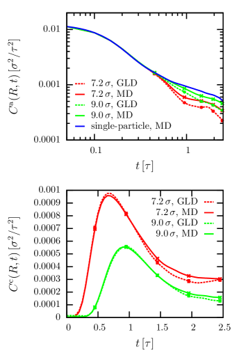
Figure 1: Velocity auto- and cross-correlation functions ($C^{\text{a}}$ and $C^{\text{c}}$, respectively) for pairs of nanocolloids at distances $R=7.2\sigma$ (red lines) and $R=9.0\sigma$ (green lines) in a nanocolloid suspension with density $\rho=10^{-4}\sigma^{-3}$ (volume fraction 1 %), as obtained from GLD simulations (dashed) and MD simulations (solid). The input memory kernels in the GLD simulations are determined using the highly dilute approximation described in Sec. III.1. Also shown for comparison is the single-particle autocorrelation function of an isolated nanocolloid (with no particles nearby) as obtained from MD simulations (blue solid line). To visualize the statistical errors, five data points with y-error bars are included in the curves. The error bars are smaller than the point size.

Fig. 1 compares the original results from the MD simulations with those from GLD simulations based on self- and pair-memory kernels that were derived with the previously described coarse-graining procedure. The velocity cross-correlation functions agree very well with each other. We can thus conclude that many-body effects do not have a significant influence on the cross-correlations in this system, at least for volume fractions around $1\%$. Deviations between the GLD and MD results are observable, however, in the velocity auto-correlation functions. The velocity decorrelation is significantly overestimated in the GLD simulations for both distances $R$. We explain this observation as follows: The comparison of the MD results for single isolated nanocolloids with those for systems of many colloids already shows that the velocity of a particle $i$ decorrelates more rapidly if other particles are in its vicinity (see Fig. 1, upper panel). The reason is that the other particles disturb the flow field and thus reduce the hydrodynamic backflow. When assuming the highly dilute limit, this many-body effect is attributed to one nearby nanocolloid at distance $R$ only. Consequentially, the two-particle contribution to the self-memory, $\Delta{K}^{\text{s}}(R,t)$, is overestimated in the coarse-graining procedure, which leads to the observed discrepancies. Additionally, the neglect of the conservative force in Eq. 22 can also have an influence on the observed discrepancies between the GLD and MD results as has recently been pointed out in Refs. (40) and (41). In our simulations, however, we found that this effect was relatively small.

To determine a coarse-grained model that accurately reproduces the MD results, one must thus combine the iterative memory reconstruction with multiparticle GLD simulations.

III.2 Accounting for many-body effects in non-Markovian coarse-grained models

In this subsection, we will show how to apply the IMRV method for the reconstruction of the frequency-dependent hydrodynamic interactions between freely diffusing nanocolloids in many-body systems. In the IMR schemes, the memory kernel $K(t)$ in the CG model is iteratively adjusted according to a prescription Jung et al. (2017)

$$K_{n}\to K_{n+1}=K_{n}+h_{n}(t)\big{(}\phi(Y_{\text{MD}})-\phi(Y^{(n)}_{\text{CG}})\big{)},$$ (29)

such that differences of the target property, $Y$, in the CG model and in the fine-grained MD model are successively reduced. Here $h_{n}(t)$ is a filter function that changes from one iteration to the next (see Ref. (23)), and $\phi(Y)$ is a mapping function, which must be optimized depending on the choice of $Y$. Specifically, the IMRV method targets the velocity correlation functions. In Ref. (23), a mapping function based on the second time derivative of $Y(t)$ was proposed. However, when applying this scheme to the present multiparticle system, we sometimes observed an accumulation of errors in $Y_{\text{CG}}(t)$ at late times that increased linearly with $t$. A better result was obtained with the alternative mapping function

$$\phi(Y)=-\alpha\frac{M^{2}}{k_{\text{B}}T}\frac{Y(t+\Delta t_{\text{}})-Y(t)}{\Delta t_{\text{}}},$$ (30)

where $\alpha\approx 6\,\tau^{-1}$ is a relaxation parameter that depends, i.a., on the nanocolloid density and the time step and needs to be adjusted for every reconstruction.

We should mention that we focus in the present work on the hydrodynamic regime in which at least a few solvent particles are located between the surfaces of the colloids, i.e., we disregard lubrication forces in the GLD simulations. This can be implemented by applying a lower cutoff $r_{\text{c,min}}=6.8\,\sigma$ to the memory kernels. For distances $R<6.8\,\sigma$, the memory kernels are replaced by the ones at $R=r_{\text{c,min}}$. The exclusion of lubrication forces is motivated by two observations: First, for small distances, the statistics of the correlation functions are worse than for larger distances, since the number of neighbors at a distance $R$ of a colloid scales quadratically with $R$. Additionally, the radial distribution function is significantly smaller than 1 in the regime $R<6.8\,\sigma$. Second, the lubrication forces lead to very strong pair interactions between the particles, which contradicts some assumptions made in this work. For example, in this case, the distance-dependence of the memory kernel cannot be assumed to be negligible on the time scale of the memory $\tau_{\text{mem}}$. The neglect of lubrication forces can of course have an influence on the overall rheological properties of the system (as has, e.g., been discussed recently in Ref. (42)). However, their influence on the long-range dynamics should be small. We are therefore confident that this assumption has no influence on the dynamical correlation functions reported in the present work.

The static pair-potential between the colloids is determined in a separate coarse-graining procedure using the iterative Boltzmann inversion (IBI) Reith et al. (2003). Details can be found in Appendix B and Ref. (43), Ch. 5. Since we disregard lubrication forces, the pair potential did not have a significant influence on the dynamical features studied in this work.

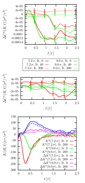
Figure 2: Illustration of the iterative memory reconstruction (IMRV) method applied to dispersions at nanocolloid density $\rho=\rho_{0}:=10^{-4}\sigma^{-3}$. The memory kernels are initialized with the results from the highly dilute approximation (Sec. III.1 and Fig. 1). The upper two panels illustrate the evolution of the differences in the velocity auto- and cross-correlation functions $C^{\text{a}}$ and $C^{\text{c}}$ between MD and GLD simulations ($\Delta C(t)=C_{\text{GLD}}(t)-C_{\text{MD}}(t)$) for particle distances $R=7.2\sigma$ (red) and $R=9\sigma$ (green) as the iteration progresses. The lower panel shows the corresponding memory kernels. To visualize the statistical errors, five data points with y-error bars are included in the curves.

The results of the iterative procedure described in this subsection are shown in Fig. 2. The reconstruction time step is $\Delta t=0.05\,\tau$ and the time scale of the correction in the iterative reconstruction $t_{\text{cor}}=0.05\,\tau$ (see Ref. (23) for details). Iterations $101-200$ correspond to an iterative reconstruction initialized with the final memory kernels of the first reconstruction (It.$~{}0-100$). The two upper panels visualize the iteration procedure. While the velocity cross-correlation functions $C^{\text{c}}$ are only subject to minor corrections if multiparticle effects are taken into account, the autocorrelation function $C^{\text{a}}$ is significantly altered. In the last iteration step, the difference between MD and GLD simulations is within the statistical errors, therefore, the iteration seems to have converged.

The lower figure compares the initial memory kernels determined in the highly dilute limit to the final results of the IMRV. It shows that the two-particle contribution to the self-memory, $\Delta{K}^{\text{s}}(R,t)$, is significantly reduced in dense systems. This is consistent with the previous discussions and demonstrates that the multiparticle coarse-graining procedure is indeed capable of incorporating many-body effects into the coarse-grained model, which were neglected when assuming the highly dilute limit. The figure also shows that, despite the reduction of $\Delta{K}^{\text{s}}(R,t)$, the distance-dependent correction to the single-particle self-memory kernel still considerably differs from zero and should not be ignored.

In sum, the results show that we can indeed reconstruct a dynamic coarse-grained model for nanocolloids in dispersion that can reproduce the dynamics of the underlying fine-grained system.

IV Analysis of the Non-Markovian Coarse-Grained Model

In this section we perform an in-depth analysis of the coarse-grained GLD model that was introduced in the previous section. We will show comparisons to MD simulations and theory and analyze the transferability and efficiency of the coarse-grained simulations.

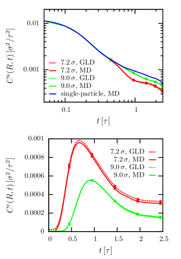
Figure 3: Same as Fig. 1, but now with GLD memory kernels obtained by full many-body IMRV reconstruction from MD simulation data at the same nanocolloid density $\rho=\rho_{0}=10^{-4}\sigma^{-3}$ (see Sec. III.2 and Fig. 2).

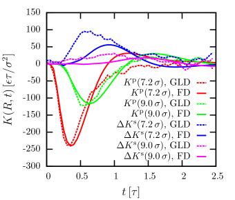
Figure 4: Two-particle contributions to the memory kernels for different particle distances $R=7.2\sigma$ and $R=9.0\sigma$ as obtained from MD simulations via many-body IMRV reconstruction (dashed lines, same data as in Fig. 2) compared to the analytical results in Ref. (25) from fluid dynamics (FD) theory. As predicted by the theory, the time scale of the peaks is $R/c_{s}$, where $c_{s}$ is the speed of sound.

IV.1 Comparison to MD simulations and hydrodynamic theory

The dynamical properties of the system, namely the velocity auto- and cross-correlation functions, are shown in Fig. 3. The results are compared to the dynamic correlation functions of the underlying microscopic model. As expected from the well-behaved convergence of the reconstruction procedure reported in the previous section, the differences between GLD and MD simulations are small. In fact, deviations can only be seen for small particle distances, $R<8.0\,\sigma$. The reason is that these small-distance correlation functions have large statistical errors which complicates the iterative memory reconstruction. Since the IMRV algorithm as applied here (Eq. (30)) only corrects for differences in the first derivative of the velocity correlation functions, it cannot easily handle constant offsets. In order to improve on this, one would have to include a term that depends on the target function $Y$ itself in the mapping function $\phi(Y)$. Alternative mapping functions, however, turned out to be less robust and since the deviations between GLD and MD simulations are small we used the previously introduced mapping function Eq. (30).

Fig. 4 compares the reproduced two-particle contributions to the self- and pair-memory kernels to analytic results from hydrodynamic theory Jung and Schmid (2017). In the case of the pair-memory kernel, the agreement is very good. Deviations are only observed for small particle distances $R<8.0\sigma$, and they can be attributed to the approximate nature of the theory at small distance to radius ratios (see discussion in Ref. (25)). In contrast, significant differences between theory and simulations can be noticed in the two-particle contribution to the self-memory kernel, $\Delta{K}^{\text{s}}(R,t)$: The self-memory is substantially underestimated by the theory. This could have two reasons: First, $\Delta{K}^{\text{s}}(R,t)$ strongly depends on the boundary condition at the surface of the colloids, since it is caused by the reflection of sound waves at nearby colloids. It is difficult to precisely model these reflections with the hydrodynamic theory. Second, as discussed in the previous section, $\Delta{K}^{\text{s}}(R,t)$ is affected by many-body effects which are not considered in the theory.

IV.2 Transferability of memory kernels

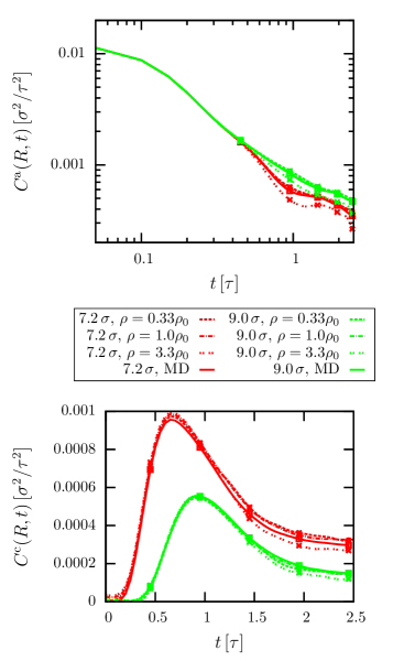
Figure 5: Same as Fig. 3, but now at different nanocolloid densities $\rho$. In the GLD simulations (dashed, dot-dashed and dotted lines), the memory kernels derived in Sec. III.2 from MD simulations at the nanocolloid density $\rho_{0}=10^{-4}\sigma^{-3}$ are used (Fig. 4). In the MD simulations, the correlation functions do not visibly depend on the density, hence only one representative curve (at $\rho=\rho_{0}$) is shown.

In the following, we study the influence of the nanocolloid density $\rho$ on the results for the velocity correlation functions. This allows us to analyze the transferability of the memory kernels determined in the previous section. All GLD simulations in this section are based on the memory kernels determined by full many-body IMRV from reference MD simulations at density $\rho=\rho_{0}$. The results are shown in Fig. 5. In the fine-grained MD system (solid line), the effect of the density on the velocity correlation functions is negligible and not visible in the plot. Similarly, a reduction of the nanoparticle density in the GLD simulations only has a minor influence on the velocity autocorrelation functions. A significant increase of the nanocolloid density, however, leads to substantial differences in the correlation functions in the GLD model, which are thus not compatible with the MD data. This can presumably be explained by the form of the self-memory kernel in Eq. (5). According to this equation, the self-memory is a sum of the single-particle contribution, $\bm{K}^{\text{s}}$, and the two-particle contributions, $\Delta\bm{K}^{\text{s}}$, of all particles that are within the cutoff $r_{\text{c}}$ of the memory kernels. If a particle $i$ is surrounded by many other particles, however, the simple sum of two-particle contributions which have been determined at a much smaller reference density is no longer appropriate. As discussed in Sec. III.2, $\Delta\bm{K}^{\text{s}}$ also includes many-body effects in an effective manner and should thus depend on the density.

The discrepancies between GLD and MD results at $\rho=3.3\rho_{0}$ shown in Fig. 5 are still comparatively small, but they increase further as $\rho$ increases. In general, the memory kernels determined at the density $\rho_{0}=10^{-4}\sigma^{-3}$ seem to be transferable to GLD simulations in the range of densities up to $\rho\lesssim 5\rho_{0}$. At even higher densities, $\rho\gtrsim 10\rho_{0}$, an additional problem emerges: In the simulations, one increasingly often encounters configurations for which the total memory tensor $\mathcal{K}$ is not positive definite. This indicates a stability problem, and moreover, the algorithm (Sec. II.3) to construct stochastic forces that satisfy the fluctuation-dissipation theorem fails. In this region the assumption made in Eq. (5) breaks down and a more sophisticated many-body description has to be found. Simply introducing density-dependent memory kernels would raise similar questions on the applicability and interpretation of these memory kernels as have been discussed for many years for the case of static pair-potentials (see e.g. Ref. (44)).

With the above analysis, we have demonstrated that the non-Markovian coarse-grained model derived in the previous section is applicable to a large range of nanocolloid densities $\rho$. The reconstructed memory kernels thus indeed characterize the fundamental hydrodynamic self- and pair-interactions between the nanocolloids. Although this sounds obvious, it is an important conclusion: By applying the iterative memory reconstruction, one can construct coarse-grained models with dynamical features that perfectly match the underlying fine-grained system, without necessarily capturing the fundamental physical features of the system. This would be the case, e.g., if the set of relevant dynamical variables chosen for the reconstruction of the coarse-grained model were not ideal. Since the Mori-Zwanzig formalism does not give any guidance regarding the optimal choice of relevant variables, this decision has to be made a posteriori and appropriately analyzed and discussed Zwanzig (2001).

IV.3 Benchmarks of the GLD simulations

The potential benefits of GLD simulations of course strongly depend on the computational costs of the simulations. We have already discussed that the algorithm scales linearly with the number of particles. Here, we will benchmark the method more quantitatively (see Table 1).

Not surprisingly, the simulation time of the fine-grained system for fixed nanocolloid number ($N=125$) strongly decreases with increasing nanocolloid density: The system contains fewer solvent particles per nanocolloid if the density goes up. In contrast, the computational costs of GLD simulations increases with increasing density, since the nanocolloids have more neighbors within their interaction range. Nevertheless, Table 1 shows that the computation time per simulation step is still significantly smaller in the GLD simulations than in the fine-grained MD simulations in all situations considered here. Furthermore, the time step in the GLD simulations is larger, which further speeds up the simulations. In total, the speedup of the systems considered in this work ranges from $S_{\text{u}}=1017\Delta t_{\text{GLD}}/\Delta t_{\text{MD}}=5.1\cdot 10^{4}$ (for $\rho=0.33\cdot 10^{-4}\,\sigma^{-3}$, corresponding to a nanocolloid volume faction of 0.33 %) to $S_{\text{u}}=44\Delta t_{\text{GLD}}/\Delta t_{\text{MD}}=0.2\cdot 10^{4}$ (for $\rho=3.3\cdot 10^{-4}\,\sigma^{-3}$, i.e., volume fraction 3.3%). It is also interesting to compare the costs of GLD simulations with the simulation costs of a corresponding Markovian implicit-solvent model without memory kernels (labeled CG MD in Table 1). The GLD simulations are slowed down by a factor of roughly $150$ compared to the Markovian simulations. This slowdown is the prize one has to pay for including the correct dynamics according to the generalized Langevin equation. Nevertheless, the GLD simulation technique still permits to speed up simulations of nanocolloid dispersions by at least 3 orders of magnitude while capturing the correct dynamics.

	$\rho\,[\sigma^{-3}]$
Simulation method	$0.33\cdot 10^{-4}$	$1.0\cdot 10^{-4}$	$3.3\cdot 10^{-4}$
MD	$61000\pm 2000\,$s	$19500\pm 750\,$s	$6400\pm 100\,$s
GLD	$60\pm 1\,$s	$63\pm 1\,$s	$145\pm 1\,$s
CG MD	$0.35\pm 0.01\,$s	$0.56\pm 0.01\,$s	$1.19\pm 0.02\,$s

Table 1: Benchmarks of the Generalized Langevin dynamics (GLD) technique compared to molecular dynamics (MD) simulations for different nanocolloid densities $\rho$. The coarse-grained (CG) MD results refer to simulations using only the mean conservative force $F^{\text{C}}(R)$. The simulations correspond to 125 nanocolloids integrated for $10^{4}$ time steps, with time step $\Delta t_{\text{MD}}=0.001\,\tau$ and $\Delta t_{\text{GLD,CG-MD}}=0.05\,\tau$. The benchmarks were run on the Mogon I cluster (https://mogonwiki.zdv.uni-mainz.de/dokuwiki/nodes) using 1 core on an “AMD Opteron 6272” CPU.

IV.4 Final discussion and remarks

The methods proposed in this work rely on the introduction of a cutoff in the memory functions in both time and space. Since hydrodynamic interactions are long-range and have long-time tails, it is thus not possible to reproduce them in full detail with the reconstructed non-Markovian models. Methods that are able to implement long-range interactions are often based on reciprocal space calculations like the Ewald summation Ewald (1921). Due to the additional time-dependence of the memory kernels, this technique cannot be adapted to the generalized Langevin equation in a straightforward manner.

One possible way to include long-range interactions in the model could be to combine the generalized and the standard Brownian dynamics (BD) technique Ermak (1975); van Gunsteren and Berendsen (1982). The former is then used to model the frequency-dependent short-range interactions, $R<r_{\text{c}}$, between the particles, and the latter accounts for long-range interactions at $R>r_{\text{c}}$, using Ewald summation. In the most naive implementation of this scheme, the pair memory term $\bm{K}_{\bm{R},\tau}^{\text{p}}$ would jump discontinuously from $\bm{K}_{\bm{R},\tau}^{\text{p}}=\bm{K}_{\text{GLD}}^{\text{p}}(\bm{R},\tau)$ at $R<r_{\text{c}}$ to $\bm{K}_{\bm{R},\tau}^{\text{p}}=\bm{K}_{\text{BD}}^{\text{p}}(\bm{R})\>\delta(\tau)$ at $R>r_{\text{c}}$. It may also be possible to link the two regimes in a continuous manner, if it is possible to find a function $\Phi(R)$ with $\Phi(r_{\text{c}})=1$ such that $\bm{K}_{\bm{R},\tau}^{\text{p}}=\bm{K}_{\text{GLD}}^{\text{p}}(\bm{R},\tau)|_{|\bm{R}|=r_{\text{c}}}\Phi(R)$, with $\Phi(R)\int_{0}^{\infty}\text{d}\tau\bm{K}_{\text{GLD}}^{\text{p}}(\bm{R},\tau)|_{|\bm{R}|=r_{\text{c}}}=\bm{K}_{\text{BD}}^{\text{p}}(\bm{R})$ for $R>r_{\text{c}}$. With such an Ansatz, the GLD technique and Ewald summation methods could possibly be combined.

The most important aspect of the non-Markovian GLD technique introduced in the present work is that it precisely models the sound waves that mediate the hydrodynamic interaction between two nanocolloids. When performing standard Brownian dynamics simulations with instantaneous hydrodynamic interactions, two approaching nanocolloids interact via an increasing friction force that decelerates the particles. The time correlation function between the particles decays rapidly. In contrast, the self- and pair-memory kernels in the non-Markovian system generate time-delayed interactions due to the finite propagation velocity of the sound waves. The memory-kernels thus induce a long-time correlation between the velocities of the particles, which has a positive sign, indicating that the particles move in the same direction (see Fig. 3, bottom panel). An important consequence of this correlation is that two particles are less likely to approach each other. This effect is captured by GLD simulations, but not by Markovian BD simulations. Additionally, the sound waves are reflected and interact with other colloids, which also influences the collective dynamics and is not captured by BD simulation techniques. The coarse-graining techniques developed in the present paper enable us to systematically investigate such memory effects and incorporate them into non-Markovian coarse-grained models. The methods thus open up new ways for dynamical coarse-graining and for understanding dynamical processes in soft matter physics.

V Conclusion

In this work we have introduced the “Generalized Langevin dynamics” (GLD) technique, a generalization of the Brownian dynamics (BD) method that includes time-dependent friction kernels. We have applied the GLD technique to study the frequency-dependent hydrodynamic interactions between two nanocolloids in a compressible fluid. The diffusion of these nanocolloids is affected by the hydrodynamic backflow effect, i.e., the movement of the colloids induces fluid vortices that interact with themselves and other colloids at later times. Additionally, these colloids have pronounced pair-interactions mediated by sound waves. Combining the iterative memory reconstruction technique introduced in Ref. (23) with GLD simulations, we can reconstruct non-Markovian coarse-grained models that precisely reproduce these transversal and longitudinal dissipative interactions. The model has a speedup of up to $S_{\text{u}}=10^{4}$ compared to MD simulations of the underlying fine-grained system, and it is transferable to a wide range of nanocolloid densities. Additionally, we have shown that the reconstructed memory kernels are quantitatively comparable to those predicted from fluid dynamic theory Jung and Schmid (2017).

The method can be applied without further adjustments to systems where long-range dissipative interactions are not important, such as frequency-dependent dipole interactions or active particles with non-instantaneous local reorientations. In cases where long-range hydrodynamic interactions cannot be neglected, it could be combined with standard BD techniques as discussed in Sec. IV.4.

An interesting topic for future research would be the construction of an auxiliary variable expansion that describes the same generalized Langevin equation as considered in this manuscript. For example, it might be possible to adapt methods from numerical analysis concerning the construction of hidden Markov models to this problem. Such an approach might be more promising than the a posteriori fitting procedures to auxiliary variable expansions that have been proposed in the literature, since the application of the latter to distance-dependent memory kernels turned out to be difficult (see the discussion in the Appendix C).

To generalize our ideas to non-equilibrium systems, it will also be important to obtain a deeper understanding of the appropriate form of the generalized Langevin equations (GLEs) in non-equilibrium situations, e.g., using the Mori-Zwanzig projection formalism Meyer et al. (2017). In particular, the fluctuation-dissipation theorem which defines the correlations of the stochastic forces at equilibrium is not necessarily valid at non-equilibriumMeyer et al. (2017). For example, it will be violated, in systems subject to active noise. Since the main focus of soft matter research currently shifts from equilibrium to non-equilibrium systems, we expect that increasing effort will be devoted to dynamic coarse-graining in the future, and that many exciting new techniques and applications will emerge. We hope that the methods presented here will prove useful in this future research.

Appendix A Derivation of the GLD integrator equations

Our starting point is Eq. (II.2) in the main text. We proceed in several steps. In the first step, we integrate Eq. (II.2) from $t_{n}=n\Delta t$ to $t_{n+1}=t_{n}+\Delta t$. Without applying any approximation, the result is

$$M(\bm{V}_{i,n+1}-\bm{V}_{i,n}) = -\bm{K}_{0}^{\text{s}}(\bm{R}_{i,n+1}-\bm{R}_{i,n})$$

$$+\Delta\bm{P}_{i,n}^{C}+\Delta{\bm{P}_{i,n}^{D}}^{\prime}+\Delta\bm{P}_{i,n}^{R},$$

where the first term singles out the momentum change of particle $i$ in the time step $\Delta t$ due to the instantaneous single-particle friction $\bm{K}_{0}^{\text{s}}$, and the other terms summarize other contributions to the total momentum change of particle $i$. The single-particle friction term is singled out, because it often dominates. Therefore, it will incorporated in a semi-implicit integration scheme in the second step of this derivation scheme. The remaining dissipative contributions to the total momentum change are given by

$$\Delta{\bm{P}_{i,n}^{D}}^{\prime}=\Delta{\bm{P}_{i,n,0}^{D}}^{\prime\prime}-\sum_{m=1}^{m_{\text{max}}-1}\Big{(}\bm{K}_{m}^{\text{s}}\Delta\bm{R}_{i,n-m}+\Delta{\bm{P}_{i,n,m}^{D}}^{\prime\prime}\Big{)}$$ (32)

with $\Delta\bm{R}_{k,n}=(\bm{R}_{k,n+1}-\bm{R}_{k,n})$ and

$$\Delta{\bm{P}_{i,n,m}^{D}}^{\prime\prime} = \sum_{j\neq i}\int\limits_{t_{n}}^{t_{n}+\Delta t_{\text{}}}\text{d}t\>\Big{(}\bm{K}_{m}^{\text{p}}[\bm{R}_{ij}(t)]\,\bm{V}_{j}(t-m\Delta t_{\text{}})$$ (33)

$$\hskip 14.22636pt+\Delta\bm{K}_{m}^{\text{s}}[\bm{R}_{ij}(t)]\,\bm{V}_{i}(t-m\Delta t_{\text{}})\Big{)}.$$

The conservative contribution is

$$\Delta\bm{P}_{i,n}^{C}=\int_{t_{n}}^{t_{n}+\Delta t_{\text{}}}\text{d}t\>\bm{F}_{i}^{\text{C}}[\{\bm{R}_{j}(t)\}],$$ (34)

and the stochastic contributions $\Delta\bm{P}_{i,n}^{R}$ are vectors of random numbers with mean zero and correlations

$$\langle\Delta\bm{P}_{i,n+m}^{R}\Delta\bm{P}_{j,n}^{R}\rangle = k_{\text{B}}T\,a_{m}\int\limits_{t_{n+m}}^{t_{n+m}+\Delta t_{\text{}}}\text{d}t\>\bm{K}_{m}^{\text{p}}[\bm{R}_{ij}(t)]\quad:\,j\neq i$$

$$\langle\Delta\bm{P}_{i,n+m}^{R}\Delta\bm{P}_{i,n}^{R}\rangle = k_{\text{B}}T\,a_{m}\bm{K}_{m}^{\text{s}}\Delta t_{\text{}}$$

$$+\sum_{k\neq i}\int\limits_{t_{n+m}}^{t_{n+m}+\Delta t_{\text{}}}\text{d}t\>\Delta\bm{K}_{m}^{\text{s}}[\bm{R}_{ij}(t)]$$

In the second step, we construct a semi-explicit integration scheme using the approximation

$$\bm{R}_{i,n+1}-\bm{R}_{i,n}=\frac{\Delta t_{\text{}}}{2}(\bm{V}_{i,n+1}+\bm{V}_{i,n})+{\cal O}(\Delta t_{\text{}}^{3})$$ (36)

Combining (36) with (A), we obtain the following equations, which are accurate up to order ${\cal O}(\Delta t_{\text{}}^{2})$.

$$\bm{R}_{i,n+1} = \bm{R}_{i,n}+\Delta t_{\text{}}\bm{b}\>\bm{V}_{i,n}$$ (37)

$$+\frac{\Delta t_{\text{}}}{2M}\bm{b}\>(\Delta\bm{P}_{i,n}^{C}+\Delta{\bm{P}_{i,n}^{D}}^{\prime}+\Delta\bm{P}_{i,n}^{R})\>$$

$$\bm{V}_{i,n+1} = \bm{a}\bm{V}_{i,n}+\frac{1}{M}\bm{b}(\Delta\bm{P}_{i,n}^{C}+\Delta{\bm{P}_{i,n}^{D}}^{\prime}+\Delta\bm{P}_{i,n}^{R})\quad$$ (38)

where the matrices $\bm{a}$ and $\bm{b}$ are given by Eq. (13) in the main text.

In the third step, we introduce further approximations for $\Delta\bm{P}_{i,n}^{C}$ and $\Delta{\bm{P}_{i,n}^{D}}^{\prime}$ in Eqs. (37) and (38). The conservative contribution, $\Delta\bm{P}_{i,n}^{C}$, is approximated by expressions such that the error in Eqs. (37) and (38) remains of order ${\cal O}(\Delta t)^{3}$. In Eq. (37), it is sufficient to use the approximation $\Delta\bm{P}_{i,n}^{C}=\Delta t_{\text{}}\bm{F}_{i,n}^{\text{C}}+{\cal O}(\Delta t_{\text{}}^{2})$ with $\bm{F}_{i,n}^{\text{C}}=\bm{F}_{i}^{\text{C}}[\{\bm{R}_{j}(t_{n})\}]$ (see also main text). In Eq. (38), an expression of order ${\cal O}(\Delta t_{\text{}}^{2})$ is required, e.g., $\Delta\bm{P}_{i,n}^{C}=\frac{\Delta t_{\text{}}}{2}(\bm{F}_{i,n}^{\text{C}}+\bm{F}_{i,n+1}^{\text{C}})+{\cal O}(\Delta t_{\text{}}^{3})$. Here, we introduce an additional correction term of order ${\cal O}(\Delta t_{\text{}}^{3})$ which does not change the order of the algorithm, but restores the form of the quasi-symplectic ”SVVm” algorithm of Melchionna in the case of Markovian single-particle Langevin dynamics. Thus we use (see also Ref. (27))

$$\Delta\bm{P}_{i,n}^{C} = \frac{1}{2}\Big{(}(1-\frac{\Delta t_{\text{}}}{2M}\bm{K}_{0}^{\text{s}})\bm{F}_{i,n}^{\text{C}}+(1+\frac{\Delta t_{\text{}}}{2M}\bm{K}_{0}^{\text{s}})\bm{F}_{i,n+1}^{\text{C}}\Big{)}$$

$$\Rightarrow\bm{b}\Delta\bm{P}_{i,n}^{C} = \frac{\Delta t_{\text{}}}{2}(\bm{a}\bm{F}_{i,n}^{\text{C}}+\bm{F}_{i,n+1}^{\text{C}}).$$ (39)

Regarding the dissipative and stochastic contributions, $\Delta{\bm{P}_{i,n}^{D}}^{\prime}$ and $\Delta\bm{P}_{i,n}^{R}$, we assume that the two-particle contributions $\bm{K}_{m}^{\text{p}}$ and $\Delta\bm{K}_{m}^{\text{s}}$ vary sufficiently slowly as a function of $\bm{R}_{ij}(t)$ so that they are approximately constant during one time step. Hence we make the approximation

$$\left.\begin{array}[]{lcl}\Delta\bm{K}_{m}^{\text{s}}[\bm{R}_{ij}(t)]&\approx&\Delta\bm{K}_{m}^{\text{s}}[\bm{R}_{ij,n}]\\ \bm{K}_{m}^{\text{p}}[\bm{R}_{ij}(t)]&\approx&\bm{K}_{m}^{\text{p}}[\bm{R}_{ij,n}]\end{array}\right\}\;\mbox{for}\;t\in[t_{n},t_{n}+\Delta t_{\text{}}].$$ (40)

The integrals in Eq. (A) are thus replaced by $\int_{t_{n}}^{t_{n}+\Delta t_{\text{}}}\text{d}t\>\bm{K}[m][\bm{R}_{ij}(t)]\approx\Delta t_{\text{}}\bm{K}[m][\bm{R}_{ij,n}]$, and the expression for $\Delta{\bm{P}_{i,n,m}^{D}}^{\prime\prime}$ (Eq. (33)) is replaced by

$$\Delta{\bm{P}_{i,n,m}^{D}}^{\prime\prime} = -\sum_{j\neq i}\Big{(}\bm{K}_{m}^{\text{p}}[\bm{R}_{ij,n}]\,\Delta\bm{R}_{j,n-m}$$ (41)

$$\hskip 28.45274pt+\Delta\bm{K}_{m}^{\text{s}}[\bm{R}_{ij,n}]\,\Delta\bm{R}_{i,n-m}\Big{)}\qquad$$

for $m>0$. However, in order to obtain an integrator based on explicit equations for $\bm{R}_{i,n+1}$ and $\bm{V}_{i,n+1}$ in each integration step, the instantaneous friction contribution $\Delta{\bm{P}_{i,n,0}^{D}}^{\prime\prime}$ must be treated differently. Here, we make the approximation

$$\Delta{\bm{P}_{i,n,0}^{D}}^{\prime\prime}=-\Delta t_{\text{}}\sum_{j\neq i}\Big{(}\bm{K}_{m}^{\text{p}}[\bm{R}_{ij,n}]\bm{V}_{j,n}+\Delta\bm{K}_{m}^{\text{s}}[\bm{R}_{ij,n}]\bm{V}_{i,n}\Big{)}$$ (42)

This completes the set of approximations that enter the algorithm. Putting everything together, we obtain Eqs. (II.2)- (15) in the main text.

We note that in the present algorithm, the instantaneous single-particle friction contributions ($\bm{K}_{0}^{\text{s}}$) and the two-particle contributions ($\Delta\bm{K}_{0}^{\text{s}}$ and $\bm{K}_{0}^{\text{p}}$) are treated on different footings. This is because we have assumed that $\bm{K}_{0}^{\text{s}}$ dominates over the two-particle contributions, hence we include only $\bm{K}_{0}^{\text{s}}$ in the implicit part of our semi-implicit scheme. Including $\Delta\bm{K}_{0}^{\text{s}}$ and $\bm{K}_{0}^{\text{p}}$ as well is possible, but results in a scheme where high dimensional matrices have to be inverted in each time step (this can be done efficiently, e.g., via the Lanczos algorithm Hochbruck and Lubich (1997); Higham (2008); Aune et al. (2013)). In the applications considered in the present work (Sec. IV), the instantaneous two-particle contributions to the memory vanished, due to the fact that the memory effects are mediated by propagating waves in the solvent. Hence the approximation $\bm{K}_{0}^{\text{s}}\gg\Delta\bm{K}_{0}^{\text{s}},\bm{K}_{0}^{\text{p}}$ was justified.

Appendix B Simulation details

In the fine-grained reference simulations, we consider systems of $N=125$ nanocolloids in a Lennard-Jones (LJ) fluid. The LJ particles have the mass $m$ and interact via a truncated and shifted LJ potential with LJ radius $\sigma$, LJ energy amplitude $\epsilon$, and cutoff at $r_{\text{c,LJ}}=2.5\sigma$. This corresponds to a hard-core interaction with a small attractive tail. The fluid is initialized by placing LJ particles on an fcc-lattice with lattice constant $a=1.71\sigma$ and therefore a density of $\rho=0.8\sigma^{-2}$. Nanocolloids are then introduced into the system by overlaying spheres of radius $R_{c}=3\sigma$ onto the fcc-lattice, and then turning all LJ particles inside the spheres into constituents of nanocolloids. This results in nanocolloids of mass $M=80m$. Nanocolloids are rigid bodies, i.e., the relative distances of all particles forming one nanocolloid are kept fixed. Particles that are part of a nanocolloid interact with other LJ particles by purely repulsive interactions, i.e., via a truncated LJ potential with cutoff $r_{\text{c,LJ}}=\sqrt[6]{2}\sigma$. We use a cubic simulation box with periodic boundary conditions in all three dimensions and box size $L^{3}=N/\rho$, where $\rho$ is the target density of the nanocolloids. The system is equilibrated at the temperature $k_{\text{B}}T=\epsilon$ by $NVT$ simulations with a Langevin thermostat. Simulation data are then collected from molecular dynamics (MD) simulations in the $NVE$ ensemble with a time step $\Delta t_{\text{\text{MD}}}=0.001\tau$. All fine-grained simulations are performed with the simulation package Lammps Plimpton (1995, 1995).

Specifically, the memory kernels were reconstructed from nanocolloid correlation functions in reference simulations of 125 nanocolloids with box dimensions $L=107.728\sigma$, corresponding to a number density $\rho_{0}=0.0001\sigma^{-3}$ and a volume fraction of 1 %. The time step of the GLD simulations is $\Delta t_{\text{}}=0.05\tau$, and the cutoff of the memory sequence is $m_{\text{max}}=50$, corresponding to the memory scale $\tau_{\text{mem}}=2.5\tau$. The spatial discretization for the memory kernels is $\Delta R=0.2\sigma$ with a cutoff at $r_{\text{c}}=15\sigma$. From the mean thermal velocity of the nanocolloids, $v=\sqrt{M^{-1}}\approx 0.1\sigma/\tau$, one can conclude that the particles roughly diffuse over a distance $\Delta R$ on the time scale $\tau_{\text{mem}}$. Thus we may assume that two-particle contributions to the memory kernels change only slightly on this time scale, which allows us to optimize the GLD algorithm by precalculating the Fourier transforms of the memory kernels in Algorithm 1 as described in Sec. II.3.

Fig. 6 shows different steps of the iterative Boltzmann inversion (IBI) reconstruction of the static pair-potential between two nanocolloids. In the first step of the iteration (lower panel, iteration 0), one simply makes the Ansatz that the potential is the negative logarithm of the pair correlation function. At this level, it becomes negative at intermediate distances. After applying the IBI procedure, however, the resulting pair potential is purely repulsive. Hence the peak in the radial distribution function (see upper panel) is due to layering of colloids and not due to solvent-mediated attractive interactions.

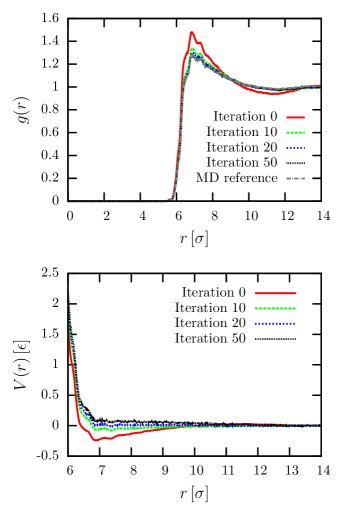
Figure 6: Iterative Boltzmann inversion (IBI) to determine the static pair-potential between two nanocolloids. The upper figure shows the different iterations of the radial distribution function $g(r)$. The gray reference curve lies precisely on top of iteration 50. The lower figure visualizes the static pair potential $V(r)$. For $r<6\,\sigma$ the potential just corresponds to a hard-core potential.

Appendix C About the auxiliary variable expansion

Most techniques that have been proposed so far to include non-Markovian dynamics into coarse-grained models are based on an auxiliary variable expansion, where the coarse-grained equations of motion are coupled to additional variables with Markovian dynamics Ceriotti et al. (2010); Córdoba et al. (2012, 2012); Baczewski and Bond (2013); Li et al. (2017). With such an approach, the non-Markovian dynamics of the system can be reproduced, although the actual equations of motion are purely Markovian. The auxiliary variables are determined by fitting (complex) exponential functions to the desired memory kernels. Unfortunately, it was not possible to adapt this procedure to the simulations considered in this work, mainly due to problems with the distance-dependent two-particle contributions to the self- and pair-memory kernels. For future reference, we shortly sketch the problems that occurred when attempting an auxiliary variable expansion.

To replace the $N$-particle generalized Langevin equation (1) with Markovian equations of motion, we use the Ansatz

$$\begin{pmatrix}\dot{\bm{V}}(t)\\ \dot{\bm{s}}(t)\end{pmatrix}=\begin{pmatrix}\bm{F}^{\text{C}}(t)\\ 0\end{pmatrix} -\begin{pmatrix}\bm{0}&\bm{A}^{vs}\\ \bm{A}^{sv}&\bm{A}^{ss}\end{pmatrix}\begin{pmatrix}\bm{V}(t)\\ \bm{s}(t)\end{pmatrix}$$

$$+\begin{pmatrix}\bm{0}&\bm{0}\\ \bm{0}&\bm{B}\end{pmatrix}\begin{pmatrix}\bm{0}\\ \zeta(t)\end{pmatrix},$$ (43)

with the auxiliary variables $\bm{s}(t)$, the coupling matrices $\bm{A}^{vs}$, $\bm{A}^{sv}$ and the dissipative matrices $\bm{A}^{ss}$. We also introduce uncorrelated Gaussian distribution random numbers $\zeta(t)$ with zero mean and unit variance. The matrices $\bm{B}$ are given by the fluctuation-dissipation theorem $\bm{B}{\bm{B}}^{\text{T}}=\bm{A}^{ss}+{\bm{A}^{ss}}^{\text{T}}$. The $2KN$-dimensional vector $\bm{s}(t)$ consists of $K$ uncoupled auxiliary variables $\bm{s}_{k}(t)$. In the following, the subscript $k=0,...,K-1$ will be used to refer to submatrices that act on the auxiliary variable $\bm{s}_{k}(t)$. Assuming that the time-dependence of $\bm{V}(t)$ is known, the set of linear equations (43) can be solved. From this we can extract the time-evolution of the auxiliary variable system,

$$\bm{s}_{k}(t)=\sum_{k=0}^{K-1}\int_{0}^{t}\text{d}t^{\prime}e^{-(t-t^{\prime})\bm{A}^{ss}_{k}}\left(\bm{A}^{sv}_{k}\bm{V}(t^{\prime})+\bm{B}_{k}\zeta_{k}(t^{\prime})\right).$$ (44)

Inserting this result into the original approach shows that Eq. (43) indeed corresponds to a generalized Langevin equation,

$$M\dot{\bm{V}}(t)=\bm{F}^{\text{C}}(t)-\sum_{k=0}^{K-1}\left(\int_{0}^{t}\text{d}s\bm{K}_{k}(t-s)\bm{V}(t)+\partial\bm{F}_{k}(t)\right).$$ (45)

The memory kernel is given by

$$\bm{K}_{k}(t)=-M\bm{A}^{vs}_{k}e^{-t\bm{A}^{ss}_{k}}\bm{A}^{sv}_{k},$$ (46)

and the correlation function of the random force is,

$$\left\langle\partial\bm{F}_{k}(t)\partial\bm{F}_{k}(t^{\prime})\right\rangle=k_{\text{B}}TM^{2}\bm{A}^{vs}_{k}e^{-(t-t^{\prime})\bm{A}^{ss}_{k}}{{\bm{A}^{vs}_{k}}^{T}}.$$ (47)

To comply with the fluctuation-dissipation theorem, we thus set $\mathbf{A}^{vs}_{k}=-M^{-1}{\mathbf{A}^{sv}_{k}}^{T}$. To simplify the notation, we also define

$$\mathbf{A}^{ss}_{k}=\begin{pmatrix}\mathbf{A}^{\prime ss}_{k}&0&0\\ 0&...&0\\ 0&0&\mathbf{A}^{\prime ss}_{k}\end{pmatrix}\quad\text{with}\quad\mathbf{A}^{\prime ss}_{k}=\begin{pmatrix}q_{k}&r_{k}\\ -r_{k}&q_{k}\end{pmatrix},$$ (48)

and introduce the reduced $N\times N$-dimensional coupling matrices $\bm{A}^{\prime sv}_{k}$,

$$A^{sv}_{k,ij} =A^{\prime sv}_{k,(2i)j}\text{ for even }i,$$ (49)

$$A^{sv}_{k,ij} =0\hskip 28.02597pt\text{ for odd }i.$$ (50)

The latter definition transfers the complex exponential functions to scalar exponential functions multiplied by a cosine. In general, it is also possible to introduce an additional phase parameter to the memory kernel. In our system, however, this complicates the fitting procedure without significantly increasing the quality of the fits. These considerations finally lead to memory kernels,

$$\mathbf{K}_{k}(t)={\mathbf{A}^{\prime sv}_{k}}^{T}{\mathbf{A}^{\prime sv}_{k}}e^{-q_{k}t}\cos(r_{k}t)=\mathbf{P}_{k}e^{-q_{k}t}\cos(r_{k}t).$$ (51)

The coupling matrices $\bm{A}^{\prime sv}_{k}$ can be calculated from $\bm{P}_{k}$ by Cholesky decomposition. These fitting matrices $\bm{P}_{k}$ contain the information about the amplitudes of the exponential functions that are fitted to the self- and pair-memory kernels.

We tested this approach for the memory kernels that were reconstructed from the fine-grained simulations. In these tests, we observed that including the self- and pair-memory kernels resulted in fitting matrices $\bm{P}^{k}$ that were not positive definite. Consequentially, the coupling matrices were not well defined. This can be rationalized in the following way: While the memory kernels themselves vary smoothly with the distances of particles, the fitting procedure produced strongly discontinuous distance-dependent amplitudes. These discontinuities could lead to impossible correlation matrices for some auxiliary variables $k$, in which one particle was strongly correlated with the other particles, while these other particles were anti-correlated. The problem could be reduced by constraining the fitting parameters, which made the fitting procedure more difficult without significantly improving the general applicability of the technique. For our systems, we were thus not able to construct a realistic and stable auxiliary variable expansion.

One possible solution for this problem could be to construct hidden Markov models directly from the atomistic simulations and not based on an a posteriori fitting procedure Baum and Petrie (1966). This, however, goes beyond the scope of the present work.

References

- Frembgen-Kesner and Elcock (2009) Frembgen-Kesner, T.; Elcock, A. H. Striking Effects of Hydrodynamic Interactions on the Simulated Diffusion and Folding of Proteins. Journal of Chemical Theory and Computation 2009, 5, 242–256.
- Tomilov et al. (2013) Tomilov, A.; Videcoq, A.; Cerbelaud, M.; Piechowiak, M. A.; Chartier, T.; Ala-Nissila, T.; Bochicchio, D.; Ferrando, R. Aggregation in Colloidal Suspensions: Evaluation of the Role of Hydrodynamic Interactions by Means of Numerical Simulations. The Journal of Physical Chemistry B 2013, 117, 14509–14517.
- Palberg (1999) Palberg, T. Crystallization kinetics of repulsive colloidal spheres. Journal of Physics: Condensed Matter 1999, 11, R323–R360.
- Vermant and Solomon (2005) Vermant, J.; Solomon, M. J. Flow-induced structure in colloidal suspensions. Journal of Physics: Condensed Matter 2005, 17, R187–R216.
- Ermak (1975) Ermak, D. L. A computer simulation of charged particles in solution. I. Technique and equilibrium properties. The Journal of Chemical Physics 1975, 62, 4189–4196.
- van Gunsteren and Berendsen (1982) van Gunsteren, W.; Berendsen, H. Algorithms for Brownian dynamics. Molecular Physics 1982, 45, 637–647.
- Lyubartsev and Laaksonen (1995) Lyubartsev, A. P.; Laaksonen, A. Calculation of effective interaction potentials from radial distribution functions: A reverse Monte Carlo approach. Physical Review E 1995, 52, 3730–3737.
- Reith et al. (2003) Reith, D.; Pütz, M.; Müller-Plathe, F. Deriving effective mesoscale potentials from atomistic simulations. Journal of Computational Chemistry 2003, 24, 1624–1636.
- Izvekov et al. (2004) Izvekov, S.; Parrinello, M.; Burnham, C. J.; Voth, G. A. Effective force fields for condensed phase systems from ab initio molecular dynamics simulation: A new method for force-matching. The Journal of Chemical Physics 2004, 120, 10896–10913.
- Shell (2008) Shell, M. S. The relative entropy is fundamental to multiscale and inverse thermodynamic problems. The Journal of Chemical Physics 2008, 129, 144108.
- Hijón et al. (2010) Hijón, C.; Español, P.; Vanden-Eijnden, E.; Delgado-Buscalioni, R. Mori-Zwanzig formalism as a practical computational tool. Faraday Discuss. 2010, 144, 301–322.
- Kinjo and Hyodo (2007) Kinjo, T.; Hyodo, S.-a. Equation of motion for coarse-grained simulation based on microscopic description. Physical Review E 2007, 75, 051109.
- Zwanzig (1961) Zwanzig, R. Memory Effects in Irreversible Thermodynamics. Physical Review 1961, 124, 983–992.
- Mori (1965) Mori, H. Transport, Collective Motion, and Brownian Motion. Progress of Theoretical Physics 1965, 33, 423–455.
- Zwanzig (2001) Zwanzig, R. Nonequilibrium statistical mechanics; Oxford University Press, 2001.
- Smith and Harris (1990) Smith, D. E.; Harris, C. B. Generalized Brownian dynamics. I. Numerical integration of the generalized Langevin equation through autoregressive modeling of the memory function. The Journal of Chemical Physics 1990, 92, 1304–1311.
- Ceriotti et al. (2010) Ceriotti, M.; Bussi, G.; Parrinello, M. Colored-Noise Thermostats à la Carte. Journal of Chemical Theory and Computation 2010, 6, 1170–1180.
- Córdoba et al. (2012) Córdoba, A.; Indei, T.; Schieber, J. D. Elimination of inertia from a Generalized Langevin Equation: Applications to microbead rheology modeling and data analysis. Journal of Rheology 2012, 56, 185–212.
- Baczewski and Bond (2013) Baczewski, A. D.; Bond, S. D. Numerical integration of the extended variable generalized Langevin equation with a positive Prony representable memory kernel. The Journal of Chemical Physics 2013, 139, 044107.
- Li et al. (2015) Li, Z.; Bian, X.; Li, X.; Karniadakis, G. E. Incorporation of memory effects in coarse-grained modeling via the Mori-Zwanzig formalism. The Journal of Chemical Physics 2015, 143, 243128.
- Davtyan et al. (2015) Davtyan, A.; Dama, J. F.; Voth, G. A.; Andersen, H. C. Dynamic force matching: A method for constructing dynamical coarse-grained models with realistic time dependence. The Journal of Chemical Physics 2015, 142, 154104.
- Li et al. (2017) Li, Z.; Lee, H. S.; Darve, E.; Karniadakis, G. E. Computing the non-Markovian coarse-grained interactions derived from the Mori-Zwanzig formalism in molecular systems: Application to polymer melts. The Journal of Chemical Physics 2017, 146, 014104.
- Jung et al. (2017) Jung, G.; Hanke, M.; Schmid, F. Iterative Reconstruction of Memory Kernels. Journal of Chemical Theory and Computation 2017, 13, 2481–2488.
- Meyer et al. (2017) Meyer, H.; Voigtmann, T.; Schilling, T. On the non-stationary generalized Langevin equation. The Journal of Chemical Physics 2017, 147, 214110.
- Jung and Schmid (2017) Jung, G.; Schmid, F. Frequency-dependent hydrodynamic interaction between two solid spheres. Physics of Fluids 2017, 29, 126101.
- Córdoba et al. (2012) Córdoba, A.; Schieber, J. D.; Indei, T. The effects of hydrodynamic interaction and inertia in determining the high-frequency dynamic modulus of a viscoelastic fluid with two-point passive microrheology. Physics of Fluids 2012, 24, 073103.
- Grønbech-Jensen and Farago (2013) Grønbech-Jensen, N.; Farago, O. A simple and effective Verlet-type algorithm for simulating Langevin dynamics. Molecular Physics 2013, 111, 983–991.
- Rotne and Prager (1969) Rotne, J.; Prager, S. Variational Treatment of Hydrodynamic Interaction in Polymers. The Journal of Chemical Physics 1969, 50, 4831–4837.
- Barrat and Rodney (2011) Barrat, J.-L.; Rodney, D. Portable Implementation of a Quantum Thermal Bath for Molecular Dynamics Simulations. Journal of Statistical Physics 2011, 1.
- Hochbruck and Lubich (1997) Hochbruck, M.; Lubich, C. On Krylov Subspace Approximations to the Matrix Exponential Operator. SIAM Journal on Numerical Analysis 1997, 34, 1911–1925.
- Higham (2008) Higham, N. J. Functions of Matrices; Society for Industrial and Applied Mathematics, 2008.
- Aune et al. (2013) Aune, E.; Eidsvik, J.; Pokern, Y. Iterative numerical methods for sampling from high dimensional Gaussian distributions. Statistics and Computing 2013, 23, 501–521.
- Press et al. (2007) Press, W. H.; Teukolsky, S. A.; Vetterling, W. T.; Flannery, B. P. Numerical Recipes 3rd Edition: The Art of Scientific Computing, 3rd ed.; Cambridge University Press: New York, NY, USA, 2007.
- Schnurr et al. (1997) Schnurr, B.; Gittes, F.; MacKintosh, F. C.; Schmidt, C. F. Determining Microscopic Viscoelasticity in Flexible and Semiflexible Polymer Networks from Thermal Fluctuations. Macromolecules 1997, 30, 7781–7792.
- Fricks et al. (2009) Fricks, J.; Yao, L.; Elston, T. C.; Forest, M. G. Time-Domain Methods for Diffusive Transport in Soft Matter. SIAM Journal on Applied Mathematics 2009, 69, 1277–1308.
- Shin et al. (2010) Shin, H. K.; Kim, C.; Talkner, P.; Lee, E. K. Brownian motion from molecular dynamics. Chemical Physics 2010, 375, 316–326.
- Carof et al. (2014) Carof, A.; Vuilleumier, R.; Rotenberg, B. Two algorithms to compute projected correlation functions in molecular dynamics simulations. The Journal of Chemical Physics 2014, 140, 124103.
- Lesnicki et al. (2016) Lesnicki, D.; Vuilleumier, R.; Carof, A.; Rotenberg, B. Molecular Hydrodynamics from Memory Kernels. Physical Review Letters 2016, 116, 147804.
- Lei et al. (2016) Lei, H.; Baker, N. A.; Li, X. Data-driven parameterization of the generalized Langevin equation. Proceedings of the National Academy of Sciences 2016, 113, 14183–14188.
- Carof et al. (2014) Carof, A.; Marry, V.; Salanne, M.; Hansen, J.-P.; Turq, P.; Rotenberg, B. Coarse graining the dynamics of nano-confined solutes: the case of ions in clays. Molecular Simulation 2014, 40, 237–244.
- Daldrop et al. (2017) Daldrop, J. O.; Kowalik, B. G.; Netz, R. R. External Potential Modifies Friction of Molecular Solutes in Water. Phys. Rev. X 2017, 7, 041065.
- Vázquez-Quesada et al. (2016) Vázquez-Quesada, A.; Tanner, R. I.; Ellero, M. Shear Thinning of Noncolloidal Suspensions. Phys. Rev. Lett. 2016, 117, 108001.
- Jung (Mainz, 2018) Jung, G. Coarse-Graining Frequency-Dependent Phenomena and Memory in Soft Matter Systems (PhD thesis); Mainz, 2018.
- Louis (2002) Louis, A. A. Beware of density dependent pair potentials. Journal of Physics: Condensed Matter 2002, 14, 9187.
- Ewald (1921) Ewald, P. P. Die Berechnung optischer und elektrostatischer Gitterpotentiale. Annalen der Physik 1921, 369, 253–287.
- Plimpton (1995) Plimpton, S. Fast Parallel Algorithms for Short-Range Molecular Dynamics. Journal of Computational Physics 1995, 117, 1–19.
- Plimpton (1995) Plimpton, S. Lammps (http://lammps.sandia.gov). 1995.
- Baum and Petrie (1966) Baum, L. E.; Petrie, T. Statistical Inference for Probabilistic Functions of Finite State Markov Chains. The Annals of Mathematical Statistics 1966, 37, 1554–1563.