Hydrodynamic convection in accretion discs

Abstract

The prevalence and consequences of convection perpendicular to the plane of accretion discs have been discussed for several decades. Recent simulations combining convection and the magnetorotational instability have given fresh impetus to the debate, as the interplay of the two processes can enhance angular momentum transport, at least in the optically thick outburst stage of dwarf novae. In this paper we seek to isolate and understand the most generic features of disc convection, and so undertake its study in purely hydrodynamical models. First, we investigate the linear phase of the instability, obtaining estimates of the growth rates both semi-analytically, using one-dimensional spectral computations, as well as analytically, using WKBJ methods. Next we perform three-dimensional, vertically stratified, shearing box simulations with the conservative, finite-volume code PLUTO, both with and without explicit diffusion coefficients. We find that hydrodynamic convection can, in general, drive outward angular momentum transport, a result that we confirm with ATHENA, an alternative finite-volume code. Moreover, we establish that the sign of the angular momentum flux is sensitive to the diffusivity of the numerical scheme. Finally, in sustained convection, whereby the system is continuously forced to an unstable state, we observe the formation of various coherent structures, including large-scale and oscillatory convective cells, zonal flows, and small vortices.

1 Introduction

Thermal convection – the bulk motion of fluid due to an entropy gradient – transports heat, mass, and angular momentum. There is compelling analytical, numerical, experimental, and observational evidence for convection both in the inner regions of stars and in the outer core and mantle of the Earth (Spruit et al., 1990; Aurnou et al., 2015), but its application to astrophysical discs is less clear. In particular, convection perpendicular to the plane of a disc bears marked differences to convection in most stars and planets. For example, the gravitational acceleration reverses sign at the disc midplane, and the gas supports a strong background shear flow. A third difference concerns the heat source necessary to drive the unstable entropy gradient. In stars this heat is provided by nuclear fusion, while in the Earth’s outer core convection is driven by both thermal and compositional gradients. In discs heating at the mid-plane is normally assumed to be supplied by accretion (and the associated viscous dissipation of heat). Turbulence arising from the magnetorotational instability and dissipation of large-scale density waves are two mechanisms that might convert orbital energy into the required heat. Note importantly that the fluid motions associated with these heating processes may in fact impede the onset of convection, and at the very least interact with it in non-trivial ways.

It has long been speculated that convection perpendicular to the plane of the disc influences the optically thick, high-accreting outburst phase of dwarf novae (for a succinct review, see Cannizzo (2011)). More recently, simulations of magnetorotational turbulence in stratified discs have shown that the MRI is capable of generating a convectively unstable entropy gradient. Moreover, three-dimensional, shearing box simulations with zero-net vertical magnetic flux reveal an interplay between convection and the MRI that might enhance angular momentum transport, typically quantified by the dimensionless parameter $\alpha$ (Bodo et al., 2013; Hirose et al., 2014). A similar interplay between magnetorotational instability and convection might operate in the ionized inner regions of protoplanetary discs, or during FU Orionis outbursts (Bell & Lin, 1994; Hirose, 2015).

In addition to dwarf novae and the inner regions of protoplanetary discs, hydrodynamic convection might drive activity in the weakly ionized ‘dead zones’ of protoplanetary discs where the magnetorotational instability is unlikely to operate (Armitage, 2011). Although irradiation by the central star usually results in an isothermal vertical profile in protoplanetary discs (Chiang & Goldreich, 1997; D’Alessio et al., 1998), heating by spiral density waves driven by a planet might nevertheless generate regions exhibiting a convectively unstable background equilibrium (Boley & Durisen, 2006; Lyra et al., 2016). So too might the heating from the dissipation of the strong zonal magnetic fields associated with the Hall effect (Lesur, Kunz and Fromang 2014).

As mentioned, accretion may instigate convection. But convection might drive accretion itself. Motivated by considerations of the primordial solar nebula, Lin & Papaloizou (1980) constructed a simple hydrodynamic model of a cooling young protoplanetary disk contracting towards the mid-plane. They showed that vertical convection arises if the opacity increases sufficiently fast with temperature, with the heating source initially provided by the gravitational contraction. But if convection is modeled via a mixing length theory, with an effective viscosity, the process might self-sustain: convective eddies could extract energy from the background orbital shear, and viscous dissipation of that energy might replace the initial gravitational contraction as a source of heat for maintaining convection.

In order to go beyond mixing length theory, Ruden et al. (1988) analysed linear axisymmetric modes in a thin, polytropic disc in the shearing box approximation and estimated that mixing of gas within convective eddies could result in values of $\alpha\sim 10^{-3}-10^{-2}$. They cautioned, however, that axisymmetric convective cells could not by themselves exchange angular momentum: such an exchange would have to be facilitated either by non-axisymmetric modes, or by viscous dissipation of axisymmetric modes.

Following these early investigations, a debate ensued that centered not so much on the size of $\alpha$ but rather on its sign. Dissipation of non-linear axisymmetric convective cells was investigated by Kley et al. (1993) who performed quasi-global simulations (spanning about 100 stellar radii) of axisymmetric viscous discs with radiative heating and cooling. They measured an inward flux of angular momentum, but warned that this might be due to the imposed axial symmetry and to their relatively high viscosity. Convective shearing waves were first investigated by Ryu & Goodman (1992), who concluded that linear non-axisymmetric perturbations would result in a net inward angular momentum flux at sufficiently large time. These results were questioned however by Lin et al. (1993), who examined analytically and numerically a set of localised linear non-axisymmetric disturbances in global geometry. They demonstrated that these modes could transport angular momentum outwards in some cases, and opined that the inward transport of angular momentum reported by Ryu & Goodman (1992) was an artifact of the shearing box approximation.

Interest in hydro convection waned after local non-linear 3D compressible simulations showed that it resulted in inward rather than outward angular momentum transport. Using the finite-difference code ZEUS and rigid, isothermal vertical boundaries, Stone and Balbus (1996, heareafter SB96) initialized inviscid, fully compressible, and vertically stratified shearing box simulations with a convectively unstable vertical temperature profile, and measured a time-averaged value of $\alpha\sim-4.2\times 10^{-5}$. Inward angular momentum transport was also reported by Cabot (1996) who ran simulations similar to those of SB96 but included full radiative transfer and a relatively high explicit viscosity. Analytical arguments for the inward transport of angular momentum by convection were presented by SB96 which, crucially, assumed axisymmetry, especially in the pressure field. However, in a rarely cited paper Klahr et al. (1999) presented fully compressible, three-dimensional, global simulations including explicit viscosity and radiative transfer of hydrodynamic convection in discs that gave some indication that non-linear convection in discs actually assumes non-axisymmetric patterns.

Some fifteen years later, the claims of SB96 and of Cabot (1996) were called into question: fully local shearing box simulations of Boussinesq hydrodynamic convection in discs using the spectral code SNOOPY and employing explicit diffusion coefficients indicated that the sign of angular momentum transport due to vertical convection can be reversed provided the Rayleigh number (the ratio of buoyancy to kinematic viscosity and thermal diffusivity) is sufficiently large. It would appear then that vertical convection can possibly drive outward angular momentum transport after all (Lesur & Ogilvie, 2010).

Our aim in this paper is to explore the competing results and claims concerning hydrodynamic convection in accretion discs, in particular to determine the sign and magnitude of angular momentum transport. We also isolate and characterize other generic features of convection that should be shared by multiple disc classes (dwarf novae, protoplanetary disks, etc) and by different driving mechanisms (MRI turbulence, spiral shock heating, etc). We do so both analytically and through numerical simulations, working in the fully compressible, vertically stratified shearing box approximation. We restrict ourselves to an idealised hydrodynamic set-up, omitting magnetic fields and complicated opacity transitions, and in so doing ensure our results are as general as possible.

The structure of the paper is as follows: first, in Section 2 we introduce the basic equations and provide a brief overview of the numerical code, the numerical parameters and set-up, and our main diagnostics. In Section 3 we investigate the linear behavior of the convective instability, employing both analytical WKBJ and semi-analytical spectral methods to calculate the growth rates and the eigenfunctions. In Section 4 we explore the non-linear regime through unforced simulations, in which the convection is not sustained and is permitted to decay after non-linear saturation. Because this unforced convection is a transient phenomenon which might depend on the initial conditions, in Section 5 we explore the non-linear regime through simulations of forced convection, in which the internal energy is relaxed to its initial, convectively unstable, state to mimic, possibly, the action of background MRI turbulent dissipation and optically thick radiative cooling. Finally, Section 6 summarizes and discusses the results.

2 Methods

2.1 Governing equations

We work in the shearing box approximation (Goldreich & Lynden-Bell, 1965; Hawley et al., 1995; Latter & Papaloizou, 2017), which treats a local region of a disc as a Cartesian box located at some fiducial radius $r=r_{0}$ and orbiting with the angular frequency of the disc at that radius $\Omega_{0}\equiv\Omega(r_{0})$. A point in the box has Cartesian coordinates $(x,y,z)$ which are related to the cylindrical coordinates $(r,\phi,z)$ through $x=r-r_{0}$, $y=r_{0}(\phi-\phi_{0}-\Omega_{0}t)$ and $z=z$. The equations of gas dynamics are now

$$\partial_{t}\rho+\nabla\cdot(\rho\mathbf{u})=0,$$ (1)

$$\partial_{t}\mathbf{u}+\mathbf{u}\cdot\nabla\mathbf{u}=-\frac{1}{\rho}\nabla P-2\Omega_{0}\mathbf{e}_{z}\times\mathbf{u}+\mathbf{g}_{\text{eff}}+\frac{1}{\rho}\nabla\cdot\mathbf{T},$$ (2)

$$\partial_{t}(\rho e)+\mathbf{u}\cdot\nabla(\rho e)=-\gamma\rho e\nabla\cdot\mathbf{u}+\mathbf{T}:\nabla\mathbf{u}+\xi\nabla^{2}T+\Lambda_{\text{relax}},$$ (3)

corresponding to conservation of mass, momentum and thermal energy, respectively. These equations are closed with a perfect gas equation of state $P=(\mathcal{R}/\mu)\rho T$, or, equivalently, $P=e(\gamma-1)\rho$ in terms of the specific internal energy $e$. Here $P$ is the thermal pressure of the fluid, $T$ is the temperature, $\rho$ is mass density, $\mathcal{R}$ is the gas constant, and $\mu$ is the mean molecular weight. The adiabatic index (ratio of specific heats) is denoted by $\gamma$ and is typically taken to be $\gamma=5/3$ in all our simulations. The effective gravitational potential is embodied in the tidal acceleration $\mathbf{g}_{\text{eff}}=2q\Omega_{0}^{2}x\hat{\mathbf{x}}-\Omega_{0}^{2}z\hat{\mathbf{z}}$, where $q$ is the shear rate. For Keplerian disks $q=3/2$ a value we adopt throughout the paper.

Other terms in the equations include the viscous stress tensor $\mathbf{T}\equiv 2\rho\nu\mathbf{S}$. Here $\nu$ is the kinematic viscosity, and $\mathbf{S}\equiv(1/2)[\nabla\mathbf{u}+(\nabla\mathbf{u})^{\text{T}}]-(1/3)(\nabla\cdot\mathbf{u})\mathbf{I}$ is the traceless shear tensor. The thermal conductivity is $\xi$, but in our simulations we specify thermal diffusivity $\chi$ rather than $\xi$. The former is related to the latter via $\chi=\xi/(c_{p}\rho)$ where $c_{p}$ is the specific heat capacity at constant pressure.

In some of our simulations we include heating and cooling through a thermal relaxation term $\Lambda_{\text{relax}}\equiv(\rho e-\rho_{0}e_{0})/\tau_{\text{relax}}$. This relaxes the thermal energy in each cell back to its initial state $e_{0}(z)\equiv e(z,\,t=0)$ on a time-scale given by $\tau_{\text{relax}}$. We refer to simulations run with $\Lambda_{\text{relax}}\neq 0$ as simulations of forced compressible convection. Conversely, simulations with $\Lambda_{\text{relax}}=0$ are referred to as unforced. The thermal relaxation time-scale $\tau_{\text{relax}}$ is taken to be the inverse of the linear growth rate of the convective instability.

2.2 Important parameters and instability criteria

The onset of thermal convection is controlled by the local buoyancy frequency, defined as

$$N^{2}_{B}=z\left[\frac{1}{\gamma}\frac{\partial\ln{P}}{\partial z}-\frac{\partial\ln{\rho}}{\partial z}\right]\Omega_{0}^{2}.$$ (4)

But convection is opposed by the effects of viscosity and thermal diffusivity, with the ratio of destabilising and stabilising processes quantified by the Rayleigh number

$$\text{Ra}\equiv\frac{N_{B}^{2}H^{4}}{\nu\chi},$$ (5)

where $H$ is the disk’s scaleheight (formally defined later). On the other hand, the ratio of buoyancy to shear is expressed through the Richardson number

$$\text{Ri}\equiv\frac{N_{B}^{2}}{q^{2}\Omega_{0}^{2}}.$$ (6)

But for convection perpendicular to the plane of an accretion disc, the buoyancy force is perpendicular to the direction of the background shear. Thus the Richardson number in our set-up is more an expression for the scaled intensity of $N^{2}_{B}$. Finally, the Prandtl number is defined as the ratio of kinematic viscosity to thermal diffusivity

$$\text{Pr}\equiv\frac{\nu}{\chi}.$$ (7)

When the explicit diffusion coefficients are neglected ($\nu,\chi=0$), convective instability occurs when the buoyancy frequency is negative (i.e. in regions where $N_{B}^{2}<0$). When explicit viscosity and thermal diffusivity are included, however, convective instability requires both that $N_{B}^{2}<0$, and that the Rayleigh number exceed some critical value $\text{Ra}_{c}$. Though in real astrophysical disks the viscosity is negligible, the inclusion of magnetic fields complicates the stability criterion, as does the presence of pre-existing turbulence (as might be supplied by the MRI) which itself may diffuse momentum and heat. In the latter case it may be possible to define a turbulent ‘Rayleigh number’, which must be sufficiently large so that convection resists the disordered background flow. In any case, the sign of $N_{B}^{2}$ is certainly insufficient to assign convection to MRI-turbulent flows, as is often done in recent work.

2.3 Numerical set-up

2.3.1 Codes

Most of our simulations are run with the conservative, finite-volume code PLUTO (Mignone et al., 2007). Unless stated otherwise, we employ the Roe Riemann-solver, 3rd order in space WENO interpolation, and the 3rd order in space Runge-Kutta algorithm. Other configurations are explored in Section 4. To allow for longer time-steps, we employ the FARGO scheme (Mignone et al., 2012). When explicit viscosity $\nu$ and thermal diffusivity $\chi$ are included, we further reduce the computational time by using the Super-Time-Stepping (STS) scheme (Alexiades et al., 1996). Note that due to the code’s conservative form kinetic energy is not lost to the grid but converted directly into thermal energy. Ghost zones are used to implement the boundary conditions.

We use the built-in shearing box module in PLUTO (Mignone et al., 2012). Rather than solving Equations (1)-(3) (primitive form), PLUTO solves the governing equations in conservative form, evolving the total energy equation rather than the thermal energy equation, where the total energy density of the fluid is given by $E=(1/2)\rho u^{2}+\rho e$ (kinetic + internal). In PLUTO the thermal relaxation term $\Lambda_{\text{relax}}=(\rho e-\rho_{0}e_{0})/\tau_{\text{relax}}$ is not implemented directly in the total energy equation. Instead, it is included on the right-hand-side of the thermal energy equation, which is then integrated (in time) analytically.

Finally, we have verified the results of our fiducial simulation (presented in Section 4.1) with the conservative finite-volume code ATHENA (Stone et al., 2008).

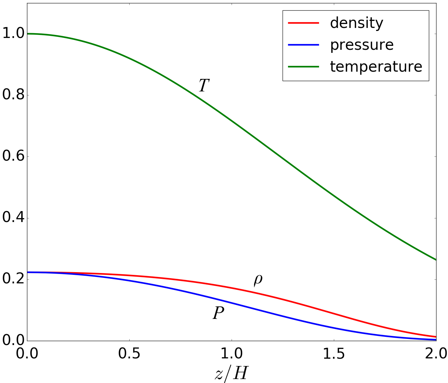
(a)

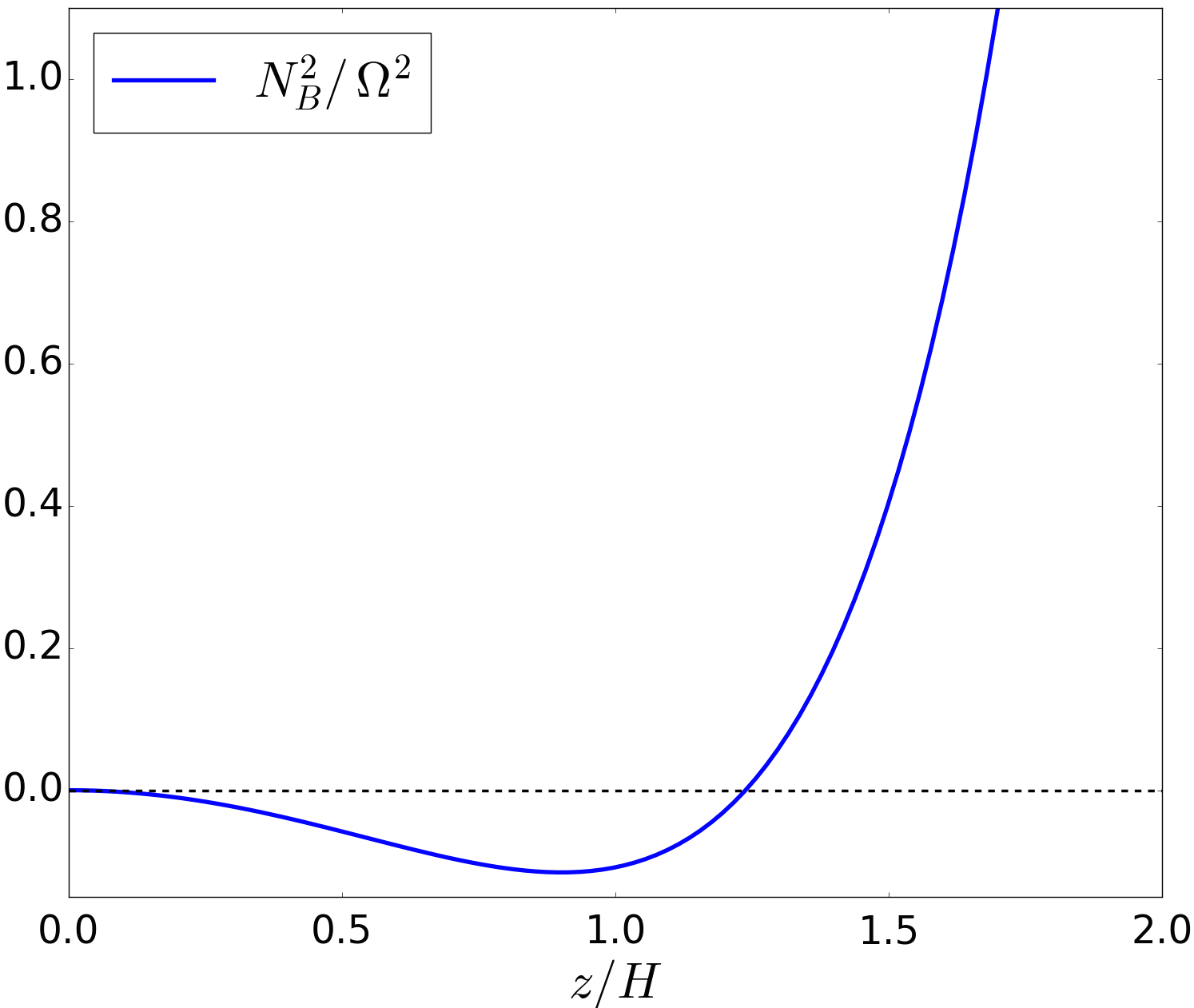
(b)

Figure 1: Vertical disc structure for Gaussian temperature profile in a disc of height $2H$ about the mid plane. Left: vertical profiles for density $\rho$, pressure $P$, and temperature $T$. Right: vertical profile of the buoyancy frequency $N_{B}^{2}/\,\Omega^{2}$. For clarity, only half of the vertical domain is shown. The profile parameters are $\{T_{0}=1.0,\rho_{0}=1.0,\beta=3.0\}$ and the adiabatic index is $\gamma=5/3$.

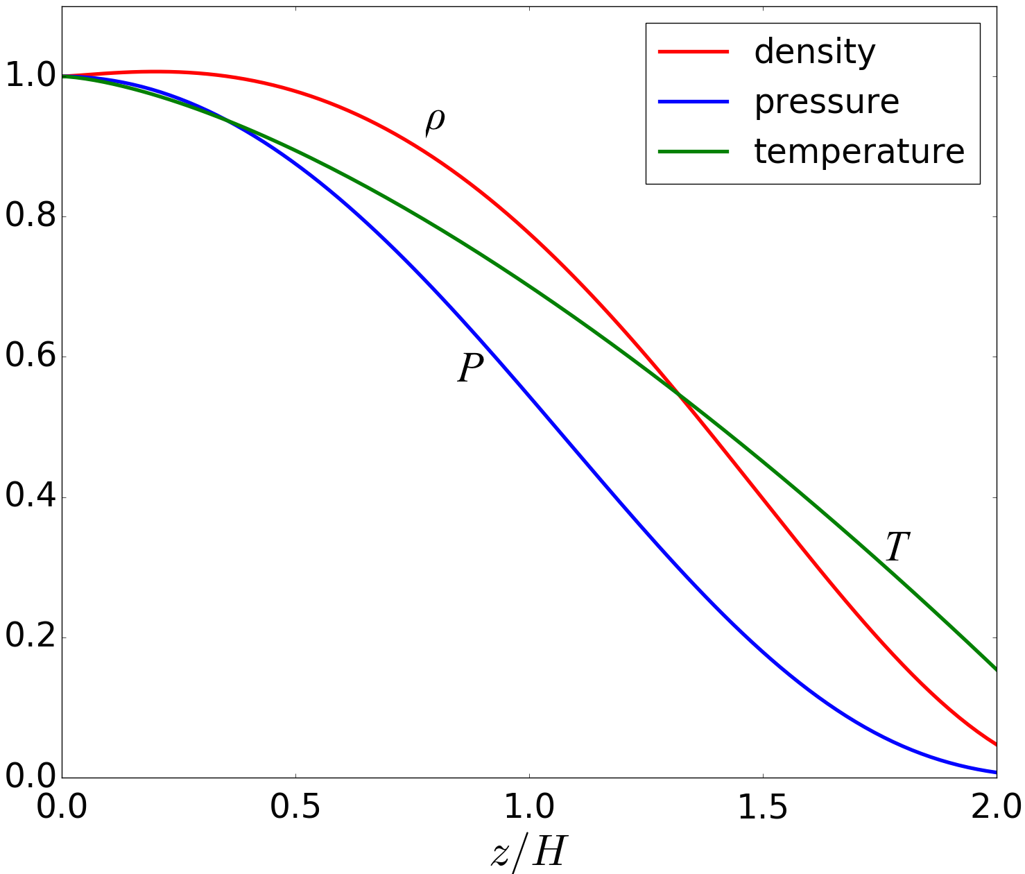
(a)

(b)

Figure 2: Vertical disc structure of Stone and Balbus (1996) in a disc of height $2H$ about the mid-plane. Left: vertical profiles for density $\rho$, pressure $P$, and temperature $T$. Right: vertical profile of the buoyancy frequency $N_{B}^{2}/\,\Omega^{2}$. For clarity, only half of the vertical domain is shown. The profile parameters are $\{T_{0}=1.0,\rho_{0}=1.0,g=5.0\}$ and the adiabatic index is $\gamma=5/3$.

2.3.2 Initial conditions and units

We use two different convectively unstable profiles to initialize our simulations. Nearly all employ an equilibrium exhibiting a Gaussian temperature profile

$$T=T_{0}\text{exp}\left[-\frac{z^{2}}{\beta H^{2}}\right],$$ (8)

where $T_{0}$ is midplane temperature and $\beta$ is a dimensionless tuning parameter. See Figure 1 for all associated thermal profiles. For comparison we also use the profile introduced by SB96 in which the temperature follows a power law

$$T=T_{0}-Az^{p},$$ (9)

where $A$ and $p$ are parameters, with $p=3/2$ usually (see Figure 2). Further details of both profiles are given in Appendix A. The equilibria are convectively unstable within a confined region (of size $L_{c}$) about the disc mid-plane, and convectively stable outside this region. We have checked that these vertical profiles are indeed good equilibrium solutions in our numerical set-up by running a series of simulations without perturbations; these show that after 55 orbits the initial profiles are unchanged with velocity fluctuation amplitudes typically less than $10^{-3}$ at the vertical boundaries and less than $10^{-7}$ at the midplane.

The background velocity is given by $\mathbf{u}=-(3/2)\Omega_{0}x\,\mathbf{e}_{y}$. At initialization we usually perturb all the velocity components with random noise exhibiting a flat power spectrum. The perturbations $\delta\mathbf{u}$ have maximum relative amplitude of about $5\times 10^{-5}$ and can be either positive or negative. In order to investigate specifically the nature of linear axisymmetric convective modes, we initialize several PLUTO simulations with linear axisymmetric modes calculated semi-analytically rather than with random noise (see Section 3.5).

Time units are selected so that $\Omega_{0}=1$. From now the subscript on the angular frequency is dropped if it appears. The length unit is chosen so that the initial midplane sound speed $c_{s}=1$, which in turn defines a constant reference scaleheight $H\equiv c_{s}/\Omega_{0}=1$. Note, however, that the sound speed is generally a function of both space and time.

2.3.3 Box size and resolution

We measure box size in units of scaleheight $H$, defined above. We employ resolutions of $64^{3},128^{3}$, $256^{3}$ and $512^{3}$ in boxes of size $4H\times 4H\times 4H$, which correspond to resolutions of 16, 32, 64 and 128 grid cells per scaleheight $H$ in all directions. However, in simulations in which we force convection we employ a ‘wide-box’ ($6H\times 6H\times 4H$) with a resolution of $256\times 256\times 256$ which corresponds to about $43$ grid cells per $H$ in the horizontal directions, and 64 grid cells per $H$ in the vertical direction.

2.3.4 Boundary conditions

We use shear-periodic boundary conditions in the $x$-direction (see Hawley et al. (1995)) and periodic boundary conditions in the $y$-direction. In the vertical direction, we keep the ghost zones associated with the thermal variables in isothermal hydrostatic equilibrium (the temperature of the ghost zones being kept equal to the temperature of the vertical boundaries at initialization) in the manner described in Zingale et al. (2002). For the velocity components we use mostly standard outflow boundary conditions in the vertical direction, whereby the vertical gradients of all velocity components are zero, and variables in the ghost zones are set equal to those in the active cells bordering the ghost zones. In a handful of our simulations we also use free-slip and periodic boundary conditions to test the robustness of our results.

2.4 Diagnostics

2.4.1 Averaged quantities

We follow the time-evolution of various volume-averaged quantities (e.g. kinetic energy density, thermal energy density, Reynolds stress, mass density, thermal pressure, and temperature). For a quantity $X$ the volume-average of that quantity is denoted $\langle X\rangle$ and is defined as

$$\langle X\rangle(t)\equiv\frac{1}{V}\int_{V}X(x,y,z,t)dV$$ (10)

where $V$ is the volume of the box.

If we are interested only in the vertical structure of a quantity $X$ then we average over the $x$- and $y$-directions, only. The horizontal average of that quantity is denoted $\langle X\rangle_{xy}$ and is defined as

$$\langle X\rangle_{xy}(z,t)\equiv\frac{1}{A}\int_{A}X(x,y,z,t)dA,$$ (11)

where $A$ is the horizontal area of the box. Horizontal averages over different coordinate directions (e.g. over the $y$- and $z$-directions) are defined in a similar manner.

We are also interested in averaging certain quantities (e.g. the Reynolds stress) over time. The temporal average of a quantity $X$ is denoted $\langle{X}\rangle_{t}$ and is defined as

$$\langle X\rangle_{t}(x,y,z)\equiv\frac{1}{\Delta t}\int_{t_{i}}^{t_{f}}X(x,y,z,t)dt,$$ (12)

where we integrate from some initial time $t_{i}$ to some final time $t_{f}$ and $\Delta t\equiv t_{f}-t_{i}$.

2.4.2 Reynolds stress, alpha, and energy densities

In accretion discs, the radial transport of angular momentum is related to the $xy$-component of the Reynolds stress, defined as

$$R_{xy}\equiv\rho u_{x}\delta u_{y}$$ (13)

where $\delta u_{y}\equiv u_{y}+q\Omega x$ is the fluctuating part of the y-component of the total velocity $u_{y}$. $R_{xy}>0$ corresponds to positive (i.e. radially outward) angular momentum transport, while $R_{xy}<0$ corresponds to negative (i.e. radially inward) angular momentum transport.

The Reynolds stress is related to the classic dimensionless parameter $\alpha$, but the reader should note that various definitions of $\alpha$ exist in the literature and care must be taken when comparing measurements of $\alpha$ quoted in different papers. We define $\alpha$ as

$$\alpha\equiv\frac{\Omega_{0}\langle R_{xy}\rangle}{q\Omega\langle P\rangle}.$$ (14)

The kinetic energy density of a fluid element is defined as

$$E_{\text{kin}}\equiv\frac{1}{2}\rho u^{2},$$ (15)

where $u$ is the magnitude of the total velocity of a fluid element. Often we will plot the vertical kinetic energy density, in which case $u$ in the above is replaced by $u_{z}$.

The total energy (kinetic plus thermal) is not conserved in the shearing box even when there are no (explicit or numerical) dissipative effects: work done by the effective gravitational potential energy on the fluid and flux of angular momentum through the $x$-boundaries due to the Reynolds stress act as sources for the total energy. The upper and lower vertical boundaries also let energy (and other quantities) leave the box.

2.4.3 Vertical profiles of horizontally averaged quantities

Finally, we track the vertical profiles of horizontally averaged pressure, density, temperature, and Reynolds stress. Of special interest is the buoyancy frequency, which is calculated from the pressure and density data by finite differencing the formula

$$\frac{N_{B}^{2}}{\Omega^{2}}=z\left[\frac{1}{\gamma}\frac{d\ln{\langle P\rangle_{xy}}}{dz}-\frac{d\ln{\langle\rho\rangle_{xy}}}{dz}\right].$$ (16)

We also calculate the (horizontally averaged) vertical profiles of mass and heat flux. We define the mass flux as

$$F_{\text{mass}}=\langle\rho u_{z}\rangle_{xy},$$ (17)

and the heat flux as

$$F_{\text{heat}}=\langle\rho u_{z}T\rangle_{xy}.$$ (18)

3 Linear theory

In this section we investigate the linear phase of the axisymmetric convective instability both semi-analytically by solving a 1D boundary value / eigenvalue problem using spectral methods, and also analytically using WKBJ methods.

Our aim is to determine the eigenvalues (growth rates) and eigenfunctions (density, velocity and pressure perturbations) of the axisymmetric convective instability in the shearing box as a function of radial wavenumber $k_{x}$. The convectively unstable background vertical profile used in all calculations is shown in Figure 1. The profile is discussed in detail in Section A.2. All calculations were carried out with profile parameters $T_{0}=1.0,\rho_{0}=1.0,\beta=3.0$ and an adiabatic index of $\gamma=5/3$. For our chosen background equilibrium, this corresponds to a Richardson number of $\text{Ri}\sim 0.05$.

We proceed as follows: first, we produce linearized equations for the perturbed variables; second, these are Fourier analyzed so that $X^{\prime}(x,z,t)=e^{\sigma t}e^{\text{i}k_{x}x}X^{\prime}(z)$ for each of the perturbed fluid variables $\rho^{\prime},\mathbf{u}^{\prime}$ and $p^{\prime}$. Here $\sigma$ can be complex (if $\sigma$ is real and positive it is referred to as a growth rate). The linearized equations are given by

$$\sigma\rho^{\prime}=-ik_{x}\rho_{0}u^{\prime}_{x}-\partial_{z}(\rho_{0}u^{\prime}_{z}),$$ (19)

$$\sigma u_{x}^{\prime}=2\Omega u^{\prime}_{y}-\frac{ik_{x}}{\rho_{0}}P^{\prime},$$ (20)

$$\sigma u^{\prime}_{y}=(q-2)\Omega u^{\prime}_{x},$$ (21)

$$\sigma u_{z}^{\prime}=-\frac{1}{\rho_{0}}\partial_{z}P^{\prime}+\frac{\rho^{\prime}}{\rho_{0}^{2}}\partial_{z}P_{0},$$ (22)

$$\begin{split}\sigma P^{\prime}&=-u^{\prime}_{z}\partial_{z}P_{0}-\gamma P_{0}(ik_{x}u^{\prime}_{x}+\partial_{z}u^{\prime}_{z}).\end{split}$$ (23)

Background fluid quantities are denoted $X_{0}=X_{0}(z)$. For equilibrium $\rho_{0}$ and $P_{0}$ see Appendix A.

3.1 Spectral methods

We discretize the fluid variables on a vertical grid containing $N_{z}$ points by expanding each eigenfunction as a linear superposition of Whittaker cardinal (sinc) functions. These are approprate as all perturbations should decay to zero far from the convectively unstable region. This choice also saves us from explicitly imposing boundary conditions. The discretised equations are next gathered up into a single algebraic eigenvalue problem (Boyd, 2001). Finally, we solve this matrix equation numerically using the QR algorithm to obtain the growth rates $\sigma$ and eigenfunctions for a given radial wavenumber $k_{x}$. The code which computes the eigensolution we often refer to as our ‘spectral eigensolver’.

3.2 WKBJ approach

Alternatively, Equations (19)-(23) can be combined into a second-order ODE of the form

$$\frac{d^{2}U}{dz^{2}}+k_{z}^{2}(z)U=0,$$ (24)

where

$$U=\left(\frac{\gamma P_{0}}{\sigma^{2}+\kappa^{2}+k_{x}^{2}c_{0}^{2}}\right)^{1/2}u_{z}^{\prime},$$ (25)

in which $c_{0}$ is the equilibrium sound speed, and the ‘vertical wavenumber’ of the perturbations is given by

$$k_{z}^{2}(z)\approx-k_{x}^{2}\frac{N_{B}^{2}(z)+\sigma^{2}}{\kappa^{2}+\sigma^{2}},$$ (26)

with $\kappa$ the epicyclic frequency (Ruden et al., 1988).

We obtain approximate solutions to Equation (24) analytically using WKBJ methods in the limit $k_{x}$ large. Equation (24) has two turning points at $k_{z}^{2}(z)=0$, which occur when $-N_{B}^{2}(z)=\sigma^{2}$. Physically, one turning point occurs at the disc mid-plane ($z=0$), while the other turning point occurs at the boundary of the convectively unstable region $z=L_{c}$. When $-N_{B}^{2}(z)>\sigma^{2}$ then $k_{z}^{2}(z)>0$ so the solutions of Equation (24) are spatially oscillatory, otherwise they are evanescent. The unstable modes, in which we are interested, are confined and oscillatory within the convectively unstable region, and spatially decay exponentially outside.

The standard WKBJ solution is given by

$$U(z)\sim c_{1}\exp{\left(+\text{i}\int^{z}k_{z}(z^{\prime})dz^{\prime}\right)}+c_{2}\exp{\left(-\text{i}\int^{z}k_{z}(z^{\prime})dz^{\prime}\right)},$$

where $c_{1}$ and $c_{2}$ are constants. By matching the interior (oscillatory) solution onto the exterior (exponentially decaying) solution, we obtain the eigenvalue equation (dispersion relation):

$$\int_{z_{0}}^{z_{1}}k_{z}(z)dz=\left(n+\frac{1}{2}\right)\pi\,\,\,\,\,\,\,\,n=0,1,2,3,\cdots,$$ (27)

where lower and upper bounds of integration $z_{0}$ and $z_{1}$, respectively, are related by the implicit equation $N_{B}^{2}(z_{0})=N_{B}^{2}(z_{1})=-\sigma^{2}$, and $n$ is the mode number. Substituting for $k^{2}_{z}(z)$ using Equation (26), we obtain an implicit equation relating the radial wavenumber $k_{x}$ and the growth rate $\sigma$ which we solve numerically via a root-finding algorithm.

3.3 Eigenvalues

For a given radial wavenumber $k_{x}$, the eigenvalues calculated with the spectral eigensolver come in pairs that lie close together in the complex plane. These correspond physically to the even and odd modes of the convective instability. As described in Section 3.4, even modes are symmetric about the mid-plane, whereas the odd modes are antisymmetric about the mid-plane. In Fig. 3 we plot as black dashed curves the first few eigenvalue branches as functions of $k_{x}$, these corresponding to vertical quantum numbers $n=0,\,1,$ and $2$. Note that in the figure $k_{x}$ has been normalized by the width of the convectively unstable region $L_{c}$ (given by Equation (32) in Appendix A.2).

As the radial wavenumber $k_{x}$ is increased, the difference between the growth rates of the even and odd modes vanishes, and the growth rates tend asymptotically to the maximum absolute value of the buoyancy frequency (indicated by a horizontal dot-dashed line). In other words, the maximum growth rate is limited by the depth of the buoyancy-frequency profile. The fastest growing modes are at arbitrarily large $k_{x}$ (small radial wavenumber $\lambda_{x}$), and thus manifest as thin elongated structures. Thicker structures are not favoured as they comprise greater radial displacements that are resisted by the radial angular momentum gradient.

Superimposed on the spectrally computed values are the WKBJ growth rates (solid lines). WKBJ methods cannot distinguish between even or odd modes, nonetheless we find very close agreement between the WKBJ and semi-analytical results for all radial wavenumbers, even at low $k_{x}$ where the WKBJ approximation is, strictly speaking, invalid. As the radial wavenumber increases, the semi-analytical and WKBJ results converge. Note that associated with each mode branch is a minimum radial wavenumber $k_{x,\text{min}}$ below which both the numerical and WKBJ growth rates are zero. This feature is just visible in the bottom left-hand side of Figure 3.

We must stress that, because the fastest growing modes are on the shortest possible scales, inviscid simulations of convection are problematic, at least in the early (linear) phase of the evolution. It is here that the simulated behaviour may depend on the varying ways that different numerical schemes deal with grid diffusion, something we explore in Section 4.3. Only with resolved physical viscosity can this problem be overcome. However, in the fully developed nonlinear phase of convection the short scale linear axisymmetric modes may be subordinate and this is less of an issue.

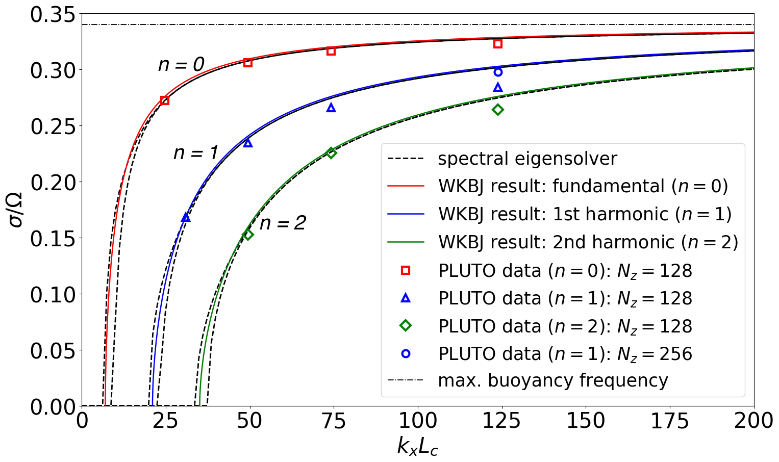
Figure 3: Growth rates as a function of radial wavenumber $k_{x}$ (scaled by the width of the convectively unstable region $L_{c}$). The solid lines were calculated analytically using WKBJ methods, and the dashed lines were calculated semi-analytically using pseudo-spectral methods. The squares, triangles, and diamonds correspond to measurements taken from PLUTO simulations run at a vertical resolution of $N_{z}=128$. The blue circle was taken from a PLUTO simulation run at $N_{z}=256$.

Figure 4: Vertical profiles of the perturbations Re$\{\rho^{\prime}(z)\}$, Re$\{u_{z}^{\prime}(z)\}$, Re$\{P^{\prime}(z)\}$, and of Im$\{u_{x}^{\prime}(z)\}$ and Im$\{u_{y}^{\prime}(z)\}$ in the upper half plane $z\in[0,2]H$, for the $n=0$ odd mode at $k_{x}=20.0$. The imaginary and real parts not shown are effectively zero. The black dot marks the upper extent of the convectively unstable region $L_{c}$, while the red dot marks the most convectively unstable points (see Equation (32)). The eigenfunctions have been rescaled so that the maximum of each eigenfunction is unity.

3.4 Vertical structure of the eigenfunctions

(a)

(b)

(c)

(d)

(e)

(f)

Figure 5: Two-dimensional profiles in the $xz$-plane of the real parts of the selected components of odd and even eigenfunctions for $n=0$ and $k_{x}=20.0$.

The reader is reminded that here we have an unstably stratified fluid in a medium in which the gravitational field smoothly changes sign. This contrasts to the more commonly studied situation of convection at the surface of the Earth (or within the solar interior). It hence is of interest to study the structure of the convective cells in some detail. We consider first the fundamental ($n=0$) odd mode with radial wavenumber $k_{x}=20$.

In Figure 4 we plot the vertical profiles of the nonzero components of the eigenfunction. To provide greater visual clarity, we have rescaled the perturbations so that the maximum amplitude of each perturbation is unity: thus we can more easily observe the vertical structure of the perturbations, but not deduce their relative amplitudes. In Figure 5 we plot their real parts in the $xz$-plane with the correct amplitudes. We find that $|u_{z}^{\prime}|>|u_{y}^{\prime}|\sim|u_{x}^{\prime}|\gg|\rho^{\prime}|\gg|P^{\prime}|$. Thus vertical velocity perturbations are greatest in magnitude, while pressure perturbations are smaller than vertical velocity perturbations by two-orders of magnitude, indicating that the convective cells are roughly in pressure balance with the surroundings, i.e that they are behaving adiabatically.

In Figure 4, $u_{z}^{\prime}$ (solid black curve) is antisymmetric about the mid-plane, whereas the remaining perturbations are symmetric about the mid-plane. Figs 4 and 5 clearly show that both odd and even modes consist of a chain of convective cells above and below the midplane and localized near the most convectively unstable point (denoted by the large red dot in the former Figure). The peak in the amplitude of $u_{z}^{\prime}$ that occurs near the this point tells us that the fluid elements reach their maximum acceleration where the buoyancy force is greatest. As the fluid perturbations behave adiabatically, they adjust their pressure to maintain a balance with the background pressure: thus where cool elements begin to rise (higher background pressure), the pressure perturbations (solid blue line) increase (i.e. $P^{\prime}>0$), and where hot elements begin to sink (lower background pressure), the pressure perturbations decrease (i.e. $P^{\prime}<0$). The vertical velocity perturbation (black solid line) is out of phase with the radial and azimuthal velocity perturbations (dashed lines), since vertical motion is converted into radial motion where the convective cells turn over (picture fluid motion at the top of a fountain).

The even modes possess a nonzero, but relatively small, $u_{z}^{\prime}$ at the midplane, and thus weakly couple the two sides of the disk. Such modes may permit some exchange of mass, momentum and thermal energy across the mid-plane when reaching large amplitudes.

As the radial wavenumber is increased from $k_{x}=20.0$ to $k_{x}=200.0$ (very small radial wavelengths), the perturbations become increasingly localized about the most convectively unstable point(s). The localisation in $z$ however is not as narrow as the radial wavelength. For larger $k_{x}$, in fact, each pair of even and odd modes change their character and become entirely localised to either the upper or lower disk. Activity in the two halves of the disk are hence completely decoupled for such small-scale (but fast growing) disturbances.

3.5 Comparison of theory with simulations

In this section we compare the growth rates previously calculated with those measured from PLUTO simulations initialized with the exact linear modes taken from the spectral eigensolver.

Table 1: Comparison of eigensolver growth rates with growth rates measured in PLUTO simulations. The simulations were initialized with the eigenfunctions corresponding to each mode $n$ and radial wavenumber $k_{x}$. All simulations except the one marked with a footnote were run at a resolution of $64\times 10\times 128$. The standard deviation on the growth rates $\sigma_{\text{PLUTO}}$ measured in the simulations is typically in the range $\pm 0.0002$ to $\pm 0.0004$.

Mode	Parity	$k_{x}$	$\sigma_{\text{EIG}}$	$\sigma_{\textsc{PLUTO}}$	$\%$ error
$n=0$	even	$20.0$	0.2727	0.2719	0.3
	odd	$20.0$	0.2724	0.2715	0.3
	even	$40.0$	0.3076	0.3059	0.6
	even	$60.0$	0.3186	0.3160	0.8
	even	$100.0$	0.3273	0.3223	1.6
$n=1$	even	$25.0$	0.1694	0.1678	0.9
	odd	$25.0$	0.1643	0.1624	0.9
	even	$40.0$	0.2392	0.2343	1.1
	even	$60.0$	0.2747	0.2655	3.3
	even	$100.0$	0.3016	0.2840	5.8
				0.2974	1.4∗
$n=2$	even	$40.0$	0.1593	0.1525	4.2
	odd	$40.0$	0.1580	0.1517	3.9
	even	$60.0$	0.2272	0.2251	0.9
	even	$100.0$	0.2749	0.2637	4

• Simulation run with a resolution of $N_{z}=256$ grid points in the vertical direction.

Each PLUTO simulation is run in a box of size $\lambda_{x}\times 0.625H\times 4H$. We maintain a fixed number of $32$ grid cells per scaleheight in the $z$-direction, $16$ grid cells per scaleheight in the $y$-direction and $64$ grid cells per radial wavelength in the $x$-direction. Thus the radial wavelength of the modes is always well resolved in our simulations. No explicit diffusion coefficients (i.e. viscosity or thermal diffusivity) are used.

The results are plotted in Figure 3 as squares (and one circle). Numerical values appear in Table 1. We find excellent agreement between simulation and theory: the relative error is $<1\%$ for the fundamental mode in the interval $k_{x}\in[20.0,60.0]$ and for the first harmonic at $k_{x}=25.0$. As the radial wavenumber is increased the simulation growth rates begin to deviate from the theoretical curves, although the percentage error remains less than $6\%$ even at large wavenumbers. This behavior is expected due to the effects of numerical diffusion which acts to decrease the growth rates as the radial wavelength approaches the size of the vertical grid. Although the radial wavenumber $\lambda_{x}$ is always well resolved in the simulations, the vertical wavelength becomes increasingly less well resolved.

The numerical diffusion could be reduced by increasing the vertical resolution of the simulations. To check this we have rerun the PLUTO simulation initialized with eigenfunctions corresponding to the first harmonic $(n=1)$ even mode with $k_{x}=100$ at twice the vertical resolution, i.e. $N_{z}=256$ instead of $N_{z}=128$. At a resolution of $N_{z}=128$ we measured a growth rate of $\sigma_{\text{PLUTO}}=0.2840\,\Omega$, corresponding to a percentage error of $5.8\%$ with the growth rate calculated semi-analytically ($\sigma_{\text{EIG}}=0.3016\,\Omega)$. At a vertical resolution of $N_{z}=256$, however, we measured a growth rate of $\sigma_{\text{PLUTO}}=0.2974\,\Omega$, corresponding to a percentage error of just $1.4\%$. Thus, the growth rates measured in the simulations appear to converge to those calculated analytically and semi-analytically as the resolution of the simulations is increased.

Finally, in all simulations of the axisymmetric modes we observed inward angular momentum transport. This is in agreement with the analytical argument presented in (Stone & Balbus, 1996) regarding axisymmetric flow.

4 Simulations of Unforced Compressible Convection

In this section we describe fully compressible, three-dimensional simulations of hydrodynamic convection in the shearing box carried out with PLUTO. These simulations are ‘unforced’ in that they are initialized with a convectively unstable profile, but this unstable profile is not maintained by a separate process (e.g. turbulent heating via the magnetorotational instability). Thus convection rearranges the profile, shifting it to a marginally stable state, and thus ultimately hydrodynamical activity dies out. While the unforced convection studied in this section is essentially a transient phenomenon that depends on initial conditions, and is sensitive to the numerical scheme (as we discuss in Sections 4.2 and 4.3), it serves as a good starting point for investigating the problem and illuminates a number of interesting features.

The key result of this section is that, even without the inclusion of explicit viscosity, we observe that hydrodynamic convection in the shearing box generally produces a positive Reynolds stress, and thus can drive outward transport of angular momentum. This is in direct contradiction to simulations carried out in ZEUS by SB96. In Section 4.1 we describe our fiducial simulations, and in Section 4.2 we compare ATHENA and PLUTO simulations. In Section 4.3 we describe the sensitivity of the sign of angular momentum transport to the numerical scheme. Finally, in Section 4.4 we investigate the effects of including explicit diffusion coefficients in our simulations, thus connecting to the Boussinesq simulations of Lesur & Ogilvie (2010).

Figure 6: Left: semi-log plot of the time-evolution of the volume-averaged vertical kinetic energy density in PLUTO simulations at resolutions of $64^{3}$ (blue line), $128^{3}$ (red line) and $256^{3}$ (black line). Right: time-evolution of volume-averaged $xy$-component of the Reynolds stress tensor.

4.1 Fiducial simulations

4.1.1 Set-up and initialization of fiducial simulations

The simulations described in this section were run at resolutions of $64^{3}$, $128^{3}$ and $256^{3}$ in boxes of size $4H\times 4H\times 4H$, where $H$ is the scaleheight. All the simulations were initialized with the convectively unstable vertical profiles for density and pressure described in Appendix A.2 with profile parameters $T_{0}=1.0,\,\rho_{0}=1.0,\,\beta=3.0$ and an adiabatic index of $\gamma=5/3$ (see Figure 1). The Stone and Balbus vertical profile SB96 was also trialled yielding very similar results, but we have omitted most of these in the interests of space. Vertical outflow conditions were employed for our fiducial simulations but periodic and free-slip boundary conditions in the vertical direction produced the same behaviour. Random perturbations to the velocity components were seeded at initialization, with a maximum amplitude $|\delta\mathbf{u}|\sim 10^{-5}$. Finally, we adopt a very small but finite thermal diffusivity of $\chi=2\times 10^{-6}$ to facilitate conduction of thermal energy through the vertical boundaries and to aid code stability. No explicit non-adiabatic heating, cooling, or thermal relaxation are included in the simulations described in this section: therefore convection gradual dies away after non-linear saturation.

4.1.2 Time-evolution of averaged quantities

In the left panel of Figure 6 we track the time-evolution of the volume-averaged kinetic energy density associated with the vertical velocity for simulations run at resolutions of $64^{3},128^{3}$ and $256^{3}$, respectively.

Initially all simulations exhibit small-amplitude oscillations due to internal gravity waves excited in the convectively stable region at initialization. After some three orbits, the linear phase of the convective instability begins in earnest, characterised by exponential growth of the perturbation amplitudes. During this phase, internal energy is converted into the kinetic energy of the rising and sinking fluid motion that comprises the convective cells. As the resolution is increased, shorter scale modes are permitted to grow. Because they are the most vigorous the growth rate (proportional to the slope of the kinetic energy density) is slightly larger at better resolution.

(a)

(b)

(c)

Figure 7: From left to right: snapshots of $u_{z}$ in the $xz$-plane taken at non-linear saturation (just after the linear phase) at resolutions of $64^{3}$, $128^{3}$ and $256^{3}$, respectively. Blue denotes $u_{z}<0$ (sinking fluid) and red denotes $u_{z}>0$ (rising fluid).

The linear phase ends some 10 orbits into the simulation, and the flow becomes especially disordered. The peak in the vertical kinetic energy density occurs at this point, but this peak decreases with resolution, something we discuss below. After non-linear saturation, the kinetic energy decreases gradually: the convective cells redistribute thermal energy and mass, thus shifting the thermal profile from a convectively unstable to a marginal state, and ultimately the convective motions die out. After about 38 orbits, the kinetic energy density has dropped to about one hundredth of its value at non-linear saturation in the lower resolution runs. The level of numerical diffusivity has an appreciable effect in damping activity after non-linear saturation, with the decrease in vertical kinetic energy successively smaller over the same period of time in the $64^{3}$, $128^{3}$ and $256^{3}$ simulations, respectively.

The behaviour of the kinetic energy aligns relatively well with our expectations. The Reynolds stress, on the other hand, is more interesting. The evolution of the $xy$-component of the Reynolds stress is plotted in the right panel of Fig. 6. The stress is small, but perhaps its most striking feature is its positivity over the entire duration of all three simulations.

Perhaps most surprising is the positivity of the stress during the linear phase of the instability. We might expect that the axisymmetric modes (which send angular momentum inwards) dominate this period of the evolution, as non-axisymmetric disturbances only have a finite window of growth (about an orbit) before they are sheared out and dissipated by the grid. But the positivity of the stress suggests that instead it is the shearing waves that are the dominant players in the linear phase. Visual inspection of the velocity fields confirms that the flow is significantly non-axisymmetric, and we find several examples of strong shearing waves ‘shearing through’ $k_{x}=0$ during this phase. It would appear these waves transport angular momentum primarily outward as they evolve from leading to trailing, behaviour that is in fact consistent with Ryu & Goodman (1992), who find that inward transport only occurs at sufficiently long times when the waves are strongly trailing and hence effectively axisymmetric. (Even then the stress is extremely oscillatory.)

Why do the shearing waves dominate over the axisymmetric modes? One hypothesis is that 3D white noise seeds fast growing shearing waves that can outcompete the axisymmetric convective instability over their permitted window of growth. If this were to be true then the simulated nonlinear regime is achieved before the dominant shearing waves become strongly trailing and begin to send angular momentum inward. Given that the typical timescale for shearing out is roughly a few orbits at best, this is marginal but not impossible. An alternative, more plausible, and more troubling hypothesis is that our inviscid numerical code misrepresents trailing shearing waves: more specifically, the code is artifically reseeding fresh leading waves from strongly trailing waves (‘aliasing’; Geoffroy Lesur, private communication). As a consequence, shearing waves outcompete the axisymmetric modes because they can shear through several times. If true, this is certainly concerning. But we hasten to add that this phenomena should only be problematic in the low amplitude linear phase; once the perturbations achieve large amplitudes the aliasing will be subsumed under physical mode-mode interactions.

The linear phase ends in a spike in the stress. Time-averages of the volume-averaged value of $R_{xy}$ from orbit 5 to orbit 15, a period spanning non-linear saturation, show that the Reynolds stress decreases as the resolution increases (see Table 2 in Appendix B). The time- and volume-averaged value of $R_{xy}$ over a period spanning non-linear saturation (orbits 5 to 15) is $+4.8\times 10^{-6}$, $+2.7\times 10^{-6}$ and $+1.7\times 10^{-6}$ in the $64^{3}$, $128^{3}$ and $256^{3}$ simulations, respectively. In terms of the turbulent alpha-viscosity this corresponds (from Equation (14)) to $\alpha\sim+2.3\times 10^{-5}$, $+1.5\times 10^{-5}$ and $9.6\times 10^{-6}$, respectively. The dependence on the numerical viscosity can be explained by appealing to secondary shear instabilities (see next subsection).

The volume-averaged density remains roughly constant during the linear phase of the instability, followed by a drop after non-linear saturation as mass is lost through the lower and upper boundaries. Although the convectively unstable region at initialization is confined to the region $|z|<L_{c}\sim 1.11H$, and is therefore well within the box, convective overshoot deposits mass (and heat) outside the convectively unstable region. The overall decrease in density over the duration of the simulation is small, but appears to increase with greater resolution. The overall percentage change in the density is $-1.4\%$, $-3.4\%$ and $-8.8\%$ in the $64^{3}$, $128^{3}$ and $256^{3}$ simulations, respectively.

4.1.3 Structure of the flow

The development of convective instability and the associated convective cells are best observed through snapshots of the vertical component of the velocity in the $xz$-plane, shown at resolutions of $64^{3},128^{3}$ and $256^{3}$ just after non-linear saturation in Figure 7. A full set of convective cells is clearly visible at all resolutions. They are thin, filamentary structures several grid cells wide comprising alternating negative and positive velocities (updrafts and downdrafts).

The maximum vertical Mach number of the flow around non-linear saturation in the $256^{3}$ run is about $M_{z}\sim 0.15$, with the largest vertical Mach numbers generally being measured near the vertical boundaries (where the temperature – and therefore the sound speed – is lowest).

The higher resolution simulations indicate that the plumes develop a wavy or buckling structure as they rise or sink, indicating the onset of a secondary shear instability. It is likely that the buckling of the convective plumes by these ‘parasitic modes’ limits the amplitudes of the linear modes, and ultimately leads to their breakdown. At lower resolution numerical diffusion smooths out the secondary shear modes, and so the convective plumes reach large amplitudes before breaking down (blue curve in right panel of Fig. 6). At high resolution the shear modes are not so impeded and make short work of these structures (black curve in the same figure).

4.1.4 Vertical heat and mass flux

Figure 8 (a) shows the vertical profiles of horizontally-averaged heat and mass fluxes taken from snapshots just after non-linear saturation from the simulation with resolution $256^{3}$. For clarity, we have time-averaged the horizontally-averaged vertical mass and heat flux profiles between orbits 5 and 10, a period spanning non-linear saturation (see Figure 6).

Negative (positive) values for the fluxes for $z<0$ and positive (negative) values for the fluxes for $z>0$ correspond to transport of heat and mass away from (towards) the mid-plane. Overall, the heat flux is away from the mid-plane, peaking in the vicinity of the most convectively unstable points at initialization (indicated by the vertical dashed red lines in Figure 8). In addition, there is some mass flux towards the mid-plane within $-H<z<H$. Thus, convection is transporting mass and heat such as to erase the convectively unstable stratification, as expected. Note that the positive peaks in the heat flux near the most convectively unstable points are similar to those observed by Hirose et al. (2014) in the thermally dominated region of the disc (i.e. $P_{\text{thermal}}>P_{\text{magnetic}}$; c.f. the middle-panel of Figure 5 in their paper).

Beyond $|z|>H$, the mass flux is directed away from the mid-plane, peaking just beyond the point which marks the boundary of the convectively unstable region. This outward mass flux might be due to convective overshoot, although we expect this effect to vanish if averaged over a suitable time interval. Alternatively, it is possible that heat transported towards the corona by the convective cells causes matter in the corona to heat up and become buoyant, or else that this heat generates a weak thermal wind.

(a)

(b)

Figure 8: (a) Vertical profiles of the vertical heat (solid red line) and mass flux (dashed black line). The outer vertical dashed (blue) lines mark the boundaries of the convectively unstable region at initialization, while the inner vertical dashed (red) lines mark the most convectively unstable points at initialization. (b) Vertical profile of the $xy$-component of the Reynolds stress tensor $R_{xy}$. In all cases, the results have been time-averaged between orbits 5 and 10, spanning non-linear saturation.

Finally, in Figure 8 (b) we show the vertical profile of the horizontally-averaged $R_{xy}$ taken from the $256^{3}$ simulation and time-averaged between orbits 5 and 10. The Reynolds stress is clearly positive over all of the vertical domain, peaking just beyond the most convectively unstable points. Thus the bulk of outward angular momentum transport occurs where the convective cells begin to turn-over, resulting in radial mixing of the gas. Note, however, that we also observe rather large positive stresses near the vertical boundaries, with the stress at the vertical boundaries about 1.5 times the peak stress in the remainder of the domain.

4.2 Simulation of compressible hydro convection in ATHENA.

In the previous section we found that hydrodynamic convection in a vertically stratified shearing box in PLUTO (without explicit viscosity) can drive outward angular momentum transport. Here we verify this result using the finite-volume code ATHENA (Stone et al., 2008; Stone & Gardiner, 2010). To facilitate as close a comparison as possible between the two codes and also to the ZEUS runs of SB96, we initialize both codes with Stone and Balbus’s convectively unstable profile (see Appendix A.1). Explicit diffusion coefficients were omitted and vertical periodic boundary conditions implemented. Both simulations were run in a shearing box of size $4H\times 4H\times 4H$ and at a resolution of $64\times 64\times 64$. PLUTO and ATHENA offer somewhat different suites of numerical schemes: here we settle on a combination that is slightly more diffusive than that employed in our fiducial simulations because this combination allows for as close a match as possible. Specifically, the numerical scheme employed in ATHENA is (second-order) piecewise linear interpolation on primitive variables, the HLLC Riemann solver and MUSCL-Hancock integration. In PLUTO we use (second-order) piecewise linear interpolation on primitive variables together with a Van Leer limiter function, the HLLC Riemann solver and MUSCL-Hancock integration. The angular frequency, and the sound speed at initialization, in both simulations were set to $\Omega=10^{-3}$ and $c_{s}=10^{-3}$, respectively.

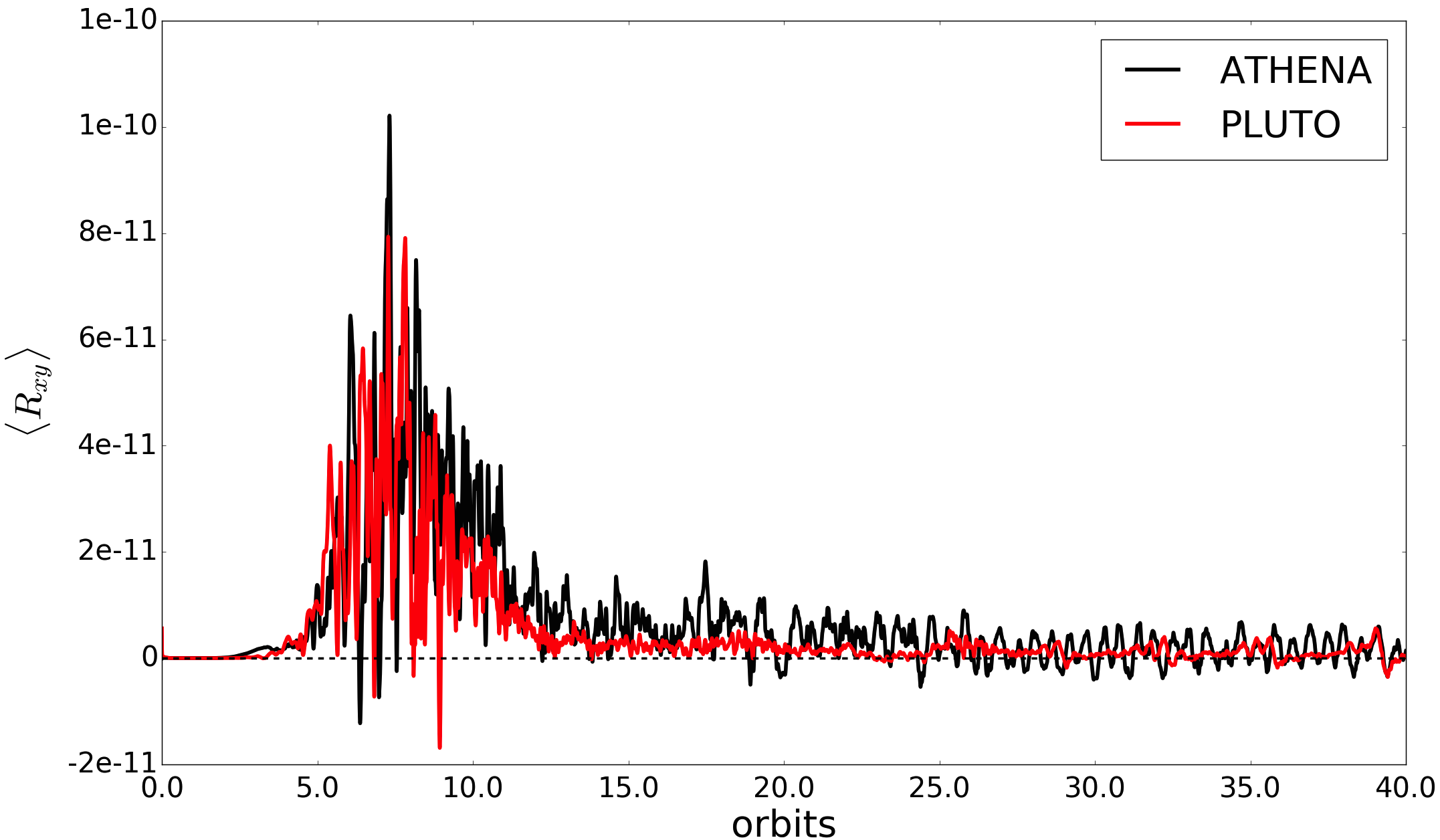
Figure 9: Comparison of time-evolution of volume-averaged Reynolds stress taken from a simulation run in ATHENA (black) with the same quantity taken from a simulation run in PLUTO (red).

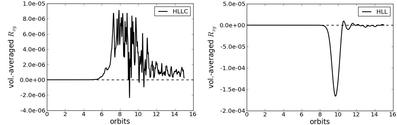
Figure 10: Left: time-evolution of volume-averaged Reynolds stress tensor taken from a PLUTO simulation run with the less diffusive HLLC solver. Right: the same, but taken from a simulation run with the more diffusive HLL solver. The change in the sign of the stress tensor provides compelling evidence that whether convection can transport angular momentum inwards or outwards depends on the diffusivity of the underlying numerical scheme.

We find that angular momentum transport is directed outwards in both codes, demonstrating that the outward transport of angular momentum by hydrodynamic convection in the non-linear phase is robust to a change of code. Figure 9 compares the time-evolution of the volume-averaged Reynolds stress taken from the ATHENA simulation with that taken from the PLUTO simulation. Both simulations exhibit exponential growth followed by non-linear saturation, together with the development of convective cells (not shown). These results also contrast with the SB96 runs with ZEUS and thus demonstrate that the positive transport reported in previous sections is not special to the Gaussian temperature profile.

Although for this particular combination of schemes the overall result is the same, we noticed that different schemes resulted in qualitative differences between the two codes. For example, when we use the HLLC solver, piecewise parabolic reconstruction (PPM) and Corner-Transport-Upwind (CTU) integration, ATHENA exhibits delayed onset of instability, a more gradual drop in kinetic energy density following non-linear saturation, and a slower drop in angular momentum transport compared to PLUTO. When we use the Roe solver, PPM reconstruction and CTU integration, the Reynolds stress is highly oscillatory in time in both codes, indicative, perhaps, of numerical instability. The different behavior (in both codes) based on which combination of numerical schemes is chosen is worrying, although we emphasize that the differences are probably accentuated by the transient nature of the evolution and its sensitivity to the initial conditions, and the fact that the linear phase is partially controlled by grid diffusion. The robustness of the results to changes is numerical scheme is investigated in more detail in the following section.

4.3 Sensitivity of sign of angular momentum transport to numerical scheme

An important result of Sections 4.1-4.2 is that purely hydrodynamic convection in PLUTO and in ATHENA resulted in $R_{xy}>0$, i.e. outward angular momentum transport. This is in disagreement with the ZEUS results of SB96, who reported a Reynolds stress of $R_{xy}<0$. Given that ZEUS is a non-conservative, finite-difference code, our hypothesis for explaining the discrepancy is that ZEUS run at comparatively low resolution (as in SB96) is sufficiently diffusive that it imposes an artificial near-axisymmetry on the flow (which will send angular momentum inward). In this section we report our attempts to assess the numerical diffusivity of various algorithms and their impact on convection.

First we reran the fiducial simulations described in Section 4.1.1 but with different combinations of numerical schemes. We found that the sign of angular momentum transport is indeed sensitive to our choice of scheme. This is best illustrated in Figure 10: the left-hand panel shows the time-evolution of the volume-averaged $R_{xy}$ taken from a simulation run with the HLLC Riemann solver, while the right-hand panel shows the same quantity but taken from a simulation run with the (more diffusive) HLL solver. Both simulations exhibit similar exponential growth in the vertical kinetic energy during the linear phase of the instability, and the velocity field shows the development of convective cells in both cases, but the sign of the Reynolds stress is radically different. The HLL run is also far more laminar and axisymmetric. We next repeated the HLL runs with higher resolutions, up to $256^{3}$, but with no change in the sign of $R_{xy}$. It must be stressed that going to higher resolutions does not necessarily help in the problem of convection; this is because the fastest growing linear modes are always near the grid scale and hence it is impossible (in the linear phase at least) to escape grid effects.

The results of different combinations of schemes is summarized in Table 3. They indicate that the sign of $R_{xy}$ appears to be robust to changes in the interpolation and time-stepping schemes, but sensitive to the Riemann solver. In particular, the less diffusive Riemann solvers (Roe and HLLC) gave $R_{xy}>0$, while the more diffusive Riemann solvers (HLL and a simple Lax-Friedrichs solver) gave $R_{xy}<0$. Altogether we explored twelve different configurations of Riemann solver, interpolation scheme, and time-stepping method. These ranged from the most accurate (least diffusive) set-up which was identical to that employed in the simulations described in the previous section (a Roe Riemann solver, third-order-in-space WENO interpolation and third-order-in-time Runge-Kutta time-stepping), to the least accurate (most diffusive) set-up (a simple Lax-Friedrich’s Riemann solver, second-order-in-space linear interpolation and second-order-in-time Runge-Kutta time-stepping).

Thus we have compelling evidence that, as suspected, angular momentum transport due to convection can be sensitive to the diffusivity of the underlying numerical scheme. It appears that over-smoothing of the flow by diffusive Riemann solvers, such as HLL, or by codes such as ZEUS that employ artificial viscosity and finite-differencing of the pressure terms, impose a spurious axisymmetry on the flow. This axisymmetry picks out the axisymmetric convective modes, which in turn transport angular momentum inwards.

4.4 Viscous simulations

Given the concerns raised in the last section regarding numerical schemes, as well as the fact that the fastest growing inviscid modes are on the shortest scales, we expand our study to include explicit viscosity (and thermal diffusivity). A properly resolved viscous simulation should exhibit none of the numerical problems encountered above, and the fastest growing mode occurs on a well defined scale above the (resolved) viscous scale. Our main aim in this section is to test whether the results of our fiducial simulations are solid: mainly, if angular momentum transport can be positive in the presence of viscosity. Additionally, the inclusion of explicit diffusion coefficients enables us to investigate the Rayleigh number dependence of fully compressible hydrodynamic convection in the shearing box, and thus connect to previous work by Lesur and Ogilvie (2010).

We carry out a suite of simulations at a resolution mainly of $256^{3}$ investigating the effects on hydrodynamic convection when the Rayleigh number Ra is increased, but the Prandtl number Pr is fixed at 2.5. Thus viscosity and thermal diffusivity each have the same magnitude in any given simulation, and we decrease both in order to increase the Rayleigh number. The Rayleigh numbers of the simulations are $\text{Ra}=10^{5},10^{6},10^{7},10^{8},10^{9}$, and $10^{10}$. (Note that the simulations undertaken at the two highest Ra are probably underresolved, as explored later.) The Richardson number at initialization is fixed by the initial vertical profile, which is described in detail in Section 4.1.1 (and shown in Figure 1). For the profile parameters chosen, the Richardson number at initialization is $\text{Ri}\sim 0.05$. Further details of the simulations are given in Table 4 in Appendix B.

4.4.1 Rayleigh number dependence

As the Rayleigh number is increased from low to high values the system proceeds through the same sequence of states found by Lesur and Ogilvie (2010). We observe no instability for $\text{Ra}=10^{5}$. At $\text{Ra}=10^{6}$ instability occurs but the flow appears relatively laminar and axisymmetric; in particular the Reynolds stress is negative througout the linear and nonlinear phases. We conclude that the critical Rayleigh number for the onset of convection lies in the range $10^{5}<\text{Ra}_{\text{c}}<10^{6}$. At $\text{Ra}=10^{7}$ the instability is more vigorous and the flow field significantly more chaotic and non-axisymmetric in the nonlinear phase, at which point the Reynolds stress has become positive. We conclude that the critical Ra at which the sign of $R_{xy}$ flips lies between $10^{6}$ and $10^{7}$. At higher Ra the flow appears even more turbulent and non-axisymmetric. It is a relief that in the nonlinear phase of the instability we find agreement with the inviscid simulations of previous sections at sufficiently high Ra.

Our critical Rayleigh number for the onset of convection is considerably higher than in Lesur & Ogilvie (2010), who report a value of $\text{Ra}_{c}=6900$, but this is perhaps explained by their much larger Richardson number $=0.2$ which remains constant throughout their box. On the other hand, the critical Ra at which $R_{xy}$ changes sign is much closer to ours, which suggests that the breakdown into non-axisymmetry may be controlled by secondary shear instabilities that are more sensitive to the viscosity than the convective driving.

While the transport of angular momentum is unambigously outward after nonlinear saturation when $\text{Ra}\geq 10^{7}$, it is almost always inwards during the linear phase, as is illustrated by the red curve in Fig. 11. Moreover, during this early stage, the simulation is dominated by the axisymmetric modes of Section 3. This disagrees with our inviscid fiducial simulations (see discussion in Section 4.1.2), which are non-axisymmetric from the outset. We confess that our viscous simulations are more in tune with our physical intuition: (a) in the linear phase growing axisymmetric modes outcompete shearing waves, (b) at sufficiently large amplitudes the modes are subject to secondary shear instabilities in the $xz$-plane that buckle the rising and falling plumes, (c) perhaps concurrently or on a short time later (and viscosity permitting), secondary non-axisymmetric instabilities also attack the plumes because they exhibit significant shear in the $xy$-plane as well, (d) at this point, the flow degenerates into something more disordered, and importantly, non-axisymmetric and the Reynolds stress flips sign. We conclude that viscosity preferentially damps shearing waves vis-a-vis axisymmetric modes, or effectively kills off the artificial aliasing of shearing waves in inviscid simulations (if this is present).

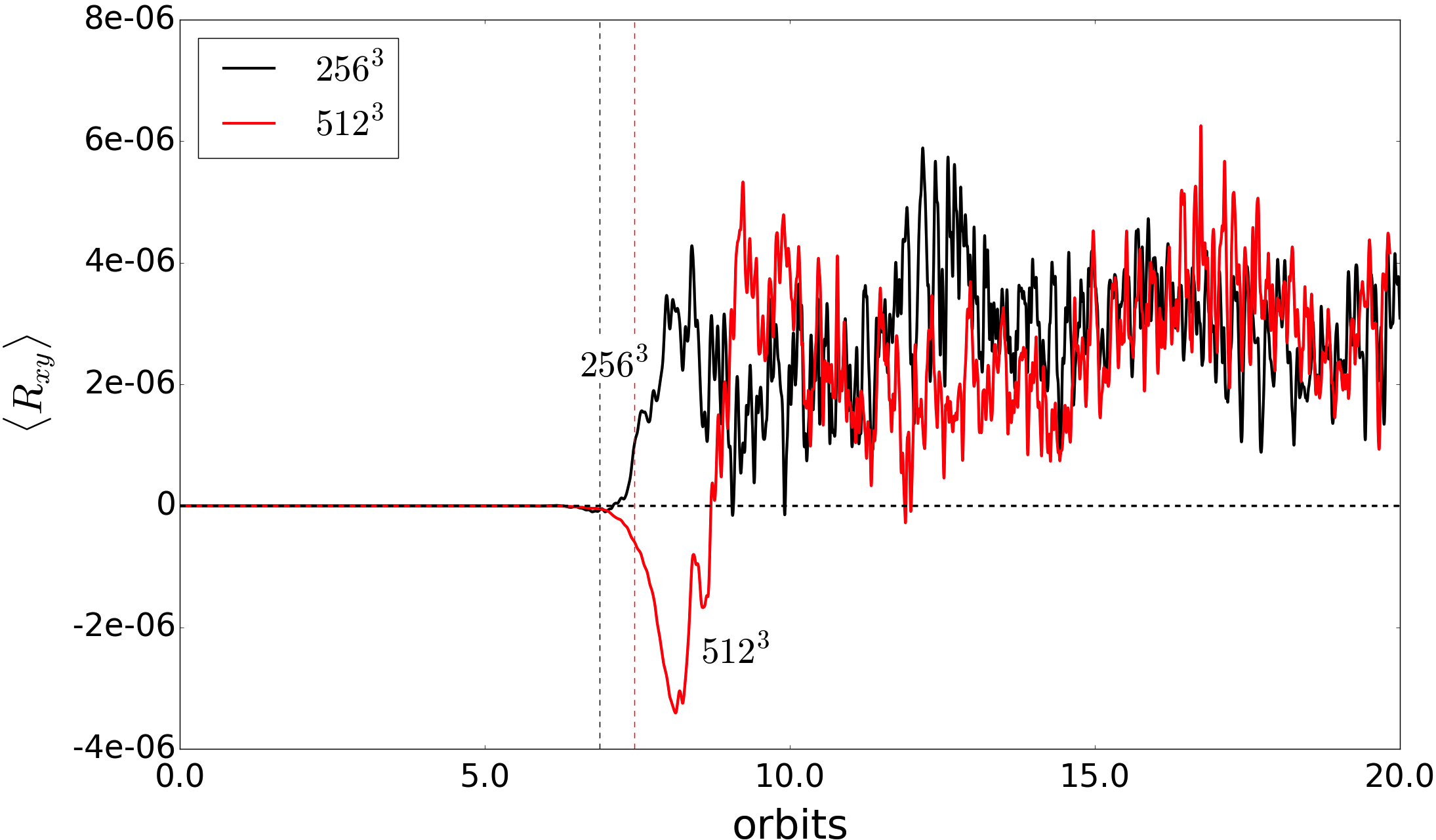
Figure 11: Time-evolution of volume-averaged $xy$-component of Reynolds stress tensor from two simulations run at resolutions of $256^{3}$ (black curve) and $512^{3}$ (red) curve at a Rayleigh number of $\text{Ra}=10^{9}$. The vertical dashed lines mark the end of the linear phase in the $256^{3}$ (black) and $512^{3}$ (red) simulations, respectively.

4.4.2 Convergence with resolution

A final issue is whether our viscous simulations are adequately resolved. More specifically: above what critical Ra is a grid of $256^{3}$ points inadequate? We conducted simulations at Ra$=10^{8}$ with $256^{3}$ and $512^{3}$ grid points and found generally good agreement between the two. The linear growth rates were almost identical and the ultimate nonlinear state statistically similar. The only noticeable difference was in the peak Reynolds stress, which was somewhat larger in the higher resolution run. Overall, we conclude that $256^{3}$ grid points are adequate to resolve a simulation with Ra$=10^{8}$.

Things start to deteriorate at a Rayleigh number of $\text{Ra}=10^{9}$. In Figure 11 we plot the time-evolution of the $xy$-component of the volume-averaged Reynolds stress for two simulations run at $256^{3}$ (black) and $512^{3}$ (red). The lower resolution run possesses no extended period of negative $R_{xy}$, in contrast to the runs at Ra$=10^{8}$. We speculate that at this resolution physical viscosity is subdominant to the grid and non-axisymmetric disturbances are artificially enhanced, probably via aliasing. At $512^{3}$, the stress is definitely negative in the linear phase and there is a strong negative peak shortly afterward. The physical viscosity is now permitted to work properly and appears to prohibit artificial non-axisymmetric disturbances. As a consequence, the axisymmetric modes preserve their control of the simulation for significantly longer and the simulation is in accord with those at lower Ra. More reassuring is the nonlinear phase a little later in which the two flows closely resemble each other. We conclude that in the linear phase $256^{3}$ is insufficient to describe a simulation of $Ra=10^{9}$, but in the later nonlinear phase it is probably adequate.

(a)

(b)

Figure 12: Left: semi-log plot of time-evolution of volume-averaged vertical kinetic energy density in a simulation with thermal relaxation. Right: time-evolution of volume-averaged $xy$-component of the Reynolds stress tensor. The thermal relaxation time was set to $\tau_{\text{relax}}=4.2\,\Omega^{-1}$.

5 Structures in forced compressible convection

In Section 4 we initialized our simulations with a convectively unstable vertical profile, but otherwise did not include any source of heating or cooling. Convection (and to a much lesser extent, conduction) transferred heat and mass vertically so as to zero the buoyancy frequency and send the box into a convectively stable equilibrium. As a result, we were only able to probe non-linear convection for a short period of time. Now we aim to continually sustain convection in order to explore this phase in greater depth. In the absence of self-sustaining convection, this means we have to maintain the convectively unstable profile artificially.

5.1 Set-up

SB96 perpetuated convection by forcing the temperature at the mid-plane to adjust to its value at initialization. This strategy, however, raises problems in conservative codes, such as PLUTO and ATHENA, because the energy injection at the midplane has no way to leave the box, except through the distant vertical boundaries (in ZEUS numerical losses on the grid supply a turbulence-dependent ‘cooling’, in addition to the cooling facilitated through the fixed-temperature boundaries). In practice, we found that the disk heats up to an inordinate level and, more importantly, it settles into a marginally unstable state, rather than a driven convective state.

Rather than forcing the code in this way, we mimic the effects of both heating and cooling through thermal relaxation. The idea is to add a source term to the energy equation such that the vertical internal energy profile relaxes to its value at equilibrium on a time-scale $\tau_{\text{relax}}$. Although this technique is artificial, it serves as a very basic tool for approximating the effects of realistic heating and cooling, as might be supplied by MRI turbulence and radiative transfer. The timescale $\tau_{\text{relax}}$ then would be the characteristic time that the radiative MRI system achieves thermodynamical quasi-equilibrium. In our simulations, however, we take the relaxation timescale to be equal to the linear growth time of convection.

In addition, to mitigate the effects of mass outflows, we incorporate a mass source term to the simulations. At the end of the $n$th time-step we calculated the total vertical mass loss through the upper and lower vertical boundaries. We then added this mass back into the box in the $(n+1)$th time-step with the same vertical profile used to initialize the density (c.f. Equation (30)).

We implement the thermal relaxation term by making slight modifications to PLUTO’s built-in optically thin cooling module. The thermal energy equation is updated during a substep to take into account user-defined sources of heating and cooling. The resolution employed in the simulation described in this section is $256\times 256\times 256$ in a box of size $6H\times 6H\times 4H$, corresponding to about $43$ grid cells per scaleheight in the $x$- and $y$-directions and $64$ grid cells per scaleheight in the vertical direction. The numerical set-up, boundary conditions and initial conditions are the same as those describe in Section 4.1.1. The thermal relaxation time is taken to be equal to the inverse of the growth rate of the convective instability which we measured to be $\sigma=0.2404\,\Omega$. Thus the thermal relaxation time is $\tau_{\text{relax}}=4.2\,\Omega^{-1}$, i.e. the internal energy is relaxed back to its equilibrium profile on about 0.7 orbits. We have also included an explicit viscosity and thermal diffusivity of $\nu=\chi=1.075\times 10^{-5}$ corresponding to a Rayleigh number of $\text{Ra}=10^{9}$ and a Prandtl number of $\text{Pr}=1$.

Finally, we have repeated the simulations in a cube of resolution $64^{3}$ and size $4H\times 4H\times 4H$, as well as at a resolution of $128\times 128\times 64$ in a box of size $6H\times 6H\times 4H$, and also with periodic boundary conditions in the vertical direction, and observed similar results. We have also run a simulation with the HLL solver to partially explore any code dependence.

(a)

(b)

(c)

(d)

(e)

(f)

Figure 13: Snapshots at different times of the $z$-component of the velocity in the $xz$-plane taken from a simulation in which convection was sustained using thermal relaxation. Narrow convective cells shown in (a) just after non-linear saturation merge to form large scale structures shown in (b), which are destroyed (c) and recreated (d) in a cyclical manner with the opposite rotation.

5.2 Large-scale oscillatory cells

In the left-hand panel of Figure 12 we show the time-evolution of the volume-averaged kinetic energy density associated with the vertical velocity. As in Section 4, exponential growth in the linear phase is followed by non-linear saturation. The forced simulations, however, do not subsequently decay. Instead the vertical kinetic energy increases at a slower rate until about orbit 20, at which point oscillations in the kinetic energy density begin to develop. The cycles increase in frequency and amplitude until about orbit 41 at which point the system settles into a quasi-equilibrium, with the volume-averaged vertical kinetic energy density oscillating about $\langle E_{\text{kin,z}}\rangle\sim 2\times 10^{-3}$ and the period remaining steady at $\Delta t=0.88$ orbits.

(a)

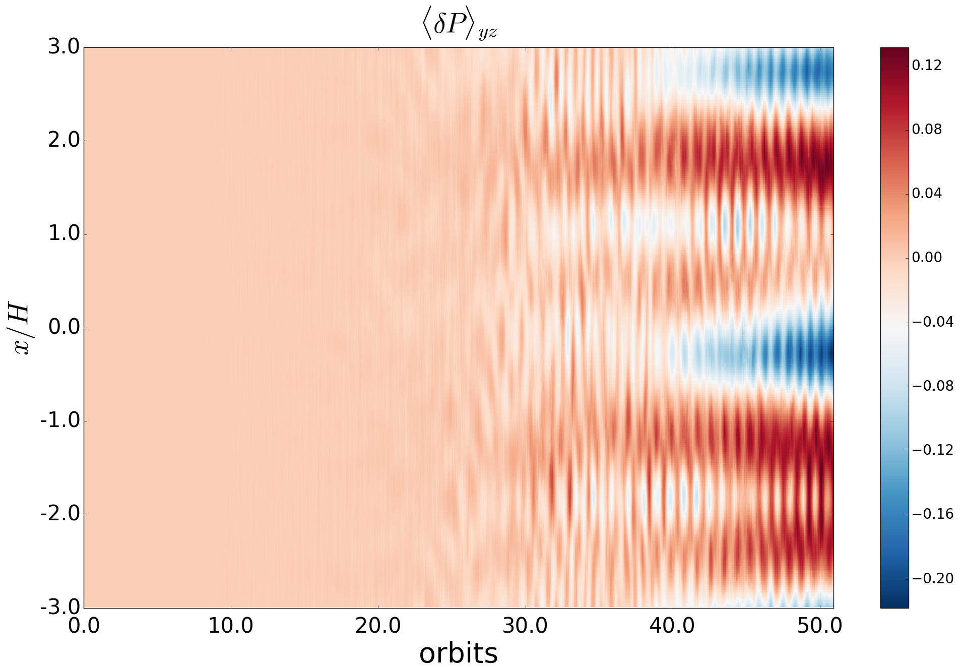
(b)

Figure 14: Space-time diagrams of $yz$-averaged $y$-component of the perturbed velocity $\delta u_{y}$ (left) and of the pressure perturbation $\delta P$ (right). (The perturbed pressure is defined in the first paragraph of Section 5.3).

Associated with the oscillations are large fluctuations in the $xy$-component of the Reynolds stress tensor (shown in the right-hand panel of Figure 12). Instantaneous fluctuations in $\langle R_{xy}\rangle$ and in $\langle\alpha\rangle$ may be either positive or negative, but the time-averaged values over this cyclical phase (orbit 20 to the end of the simulation) are $R_{xy}\sim+9.9\times 10^{-6}$ and $\alpha\sim+3.9\times 10^{-5}$, respectively. Furthermore, comparing the oscillations in the vertical kinetic energy density to the fluctuations in $\langle R_{xy}\rangle$ and also to the volume-averaged gas pressure $\langle P\rangle$ (not shown here) it is apparent that peaks in the kinetic energy density are correlated with both $\langle R_{xy}\rangle<0$ and troughs in $\langle P\rangle$, while troughs in the kinetic energy density are correlated with $\langle R_{xy}\rangle>0$ and peaks in $\langle P\rangle$.

(a)

(b)

(c)

(d)

Figure 15: Two-dimensional slices in the $xy$-plane of the perturbation to the $y$-component of the velocity $\delta u_{y}$, and of the fractional pressure perturbation $\delta P$ from a simulation of forced compressible convection at $z\approx 0.5H$. Left column: slices taken from a snapshot just after non-linear saturation (orbit 7.4). Right column: slices taken from snapshot generated during the cyclical phase (orbit 41.6).

A clearer picture of the behaviour of the system emerges when we study the structure of the flow during the cyclical phase. Figure 13 shows snapshots of the $z$-component of the velocity in the $xz$-plane. The first panel is taken just after the end of the linear phase (orbit 7.4); the subsequent panels are taken at five successive peaks and troughs in the kinetic energy. As the kinetic energy rises in the non-linear phase, the thin convective cells with radial wavelengths $\lambda_{x}\sim 5\,\Delta x\sim 0.177H$, where $\Delta x$ is the size of grid a cell in the $x$-direction, slowly begin to merge into larger coherent structures which couple the two halves of the disc together. By orbit 20 (start of the cyclical phase), the radial wavelength of the convective cells has increased to $\lambda_{x}\sim H$, and by the time the quasi-steady equilibrium state sets in (at around orbit 40) the radial wavelength of the convective cells is $\lambda_{x}\sim 3.4H$.

Comparing the snapshots of $u_{z}$ to the peaks and troughs in the kinetic energy, it becomes apparent that peaks in the convective energy are associated with the large-scale axisymmetric convective cells, hence $\alpha<0$. Troughs in the kinetic energy are associated with destruction of those convective cells and with positive stress (outward angular momentum transport). Thus we are observing large-scale convective eddies that appear to be created and destroyed cyclically. Furthermore, it is evident from Figure 13 that after the eddies are destroyed, they are re-formed with the opposite rotation.

The reader may be alarmed that the large eddies extend all the way to the vertical boundaries of the domain, and indeed there is an uncomfortable level of mass loss during this phase. To check that the flows are not an artefact of our box size, we ran additional simulations with a vertical domain of $\pm 3H$. A density floor had to be activated in such runs, which unfortunately compromised our thermal equilibrium and complicated the onset of convection early in the simulation. However, they ultimately settled onto the cyclical state described above, but now the large-scale eddies peter out before reaching the vertical boundaries. As a result, the mass loss drops to negligible amounts. This confirms that these flows are physical and robust, though only marginally contained within our smaller boxes.

Figure 16: Two-dimensional slice in the $xy$-plane of the $z$-component of the vorticity $\omega_{z}$ taken from snapshot generated at the start of the cyclical phase (orbit 20) and at $z\approx 0.5H$. For clarity we have zoomed in on the upper-right quadrant of the $xy$-plane.

Next, to explore any code dependence of this final outcome, we have rerun the simulation with the more diffusive HLL solver. We observe a negative Reynolds stress during the linear phase and well into the non-linear phase. Associated with this is a remarkably axisymmetric flow field, as confirmed by viewing slices of the pressure perturbation $\delta P$ in the $xy$-plane at different times. The simulation, nonetheless, enters the cyclical phase during which this axisymmetry is broken. As expected there is a flip in the sign of the Reynolds stress from negative to positive. The behavior thereafter mirrors that of the simulation of forced compressible convection run with the Roe solver: the cyclical creation and destruction of large scale convective cells and an oscillatory Reynolds stress. We conclude that for forced runs, the ultimate quasi-steady state depends negligibly on the algorithm.

5.3 Zonal Flows

In Figure 14 we plot, side-by-side, space-time diagrams in the $xt$-plane of the $yz$-averaged pressure perturbation $\delta P(x,t)\equiv(\langle P\rangle_{yz}-\langle P\rangle)/\langle P\rangle$ and of the $yz$-averaged perturbation to the $y$-component of the velocity $\langle\delta u_{y}\rangle_{yz}(x,t)\equiv\langle u_{y}-1.5\,\Omega\,x\rangle_{yz}$. It is immediately evident from Figure 14 that around the onset of the cyclical phase (orbit 20) alternating streaks in $\delta P$ and $\delta u_{y}$ begin to develop. Respectively, these mark alternating bands (in $x$) of high ($\delta P>0$) and low ($\delta P<0$) pressure, and of super-Keplerian ($\delta u_{y}>0$) and sub-Keplerian ($\delta u_{y}<0$) flow.

From Figure 14 it is clear that the pressure and velocity perturbations are 90 degrees out of phase, which is characteristic of zonal flows. We hesitate, however, to claim that these structures are in geostrophic balance (i.e. that $\partial_{x}P^{\prime}\sim\,\rho_{0}\,\Omega\,\delta u_{y}$) because, as is evident from the space-time diagrams, the flows are not stationary in time but appear to fluctuate over about one orbit – the same timescale over which the large convective cells are created and destroyed. Indeed the creation and destruction of the zonal flows tracks precisely that of the large-scale convective cells, showing clearly that the two phenomena are connected. The axisymmetry observed during the formation of large-scale convective cells and zonal flows is consistent with the inward transport of angular momentum observed while these structures remain coherent: axisymmetric convective modes dominate during the lifetime of these structures and transport angular momentum inwards.

In Figure 15 (right-hand panels) we plot snapshots in the $xy$-plane taken during the cyclical phase of the perturbation of the $y$-component of the velocity $\delta u_{y}$ and of the perturbed pressure $\delta P$. The axisymmetric structure of the zonal flows is clearly visible in panels (b) and (d), as is the $\pi/2$ phase difference between the pressure perturbation $\delta P$ and the perturbed $y$-component of the velocity $\delta u_{y}$.

5.4 Vortices

Because the zonal flows consist of alternating bands of sub- and super-Keplerian motion – with strong shear between the bands – we expect that they could give rise to vortices via the Kelvin-Helmholtz instability (modified by rotation and stratification). In Figure 15 we plot a snapshot in the $xy$-plane taken during the cyclical phase of the the $z$-component of the vertical component of vorticity $\omega_{z}$. Small but coherent anti-cyclonic blobs of vorticity are observed during the cyclical phase, and these occur precisely where the flow transitions from sub-Keplerian to super-Keplerian (i.e. at the edges of the zonal flows). Typically only anti-cyclonic vortices are observed, which is consistent with the fact that cyclonic vortices tend to be more unstable in Keplerian shear flows.

The vortices tend to be elongated at the start of the cyclical phase (around orbit 20), with an aspect ratio of about 0.4, and grow increasingly circular with time; in fact, once quasi-steady equilibrium has been reached at around orbit 41, many of the vortices have aspect ratios approaching unity. They appear to have limited three-dimensional extent, and we did not observe any vortices that remained coherent for depths exceeding half a scale-height.

5.5 Discussion

It is tempting to link our results to the large-scale emergent structures in recent simulations of rotating hydrodynamic convection with uniform (rather than Keplerian) rotation and in the Boussinesq (rather than compressible) regime (Favier et al., 2014; Guervilly et al., 2014). Both Favier et al. (2014) and Guervilly et al. (2014) observe growth in the vertical component of the kinetic energy at high Rayleigh numbers ($\text{Ra}\sim 10^{7}-10^{9}$), as we do. In addition, Favier et al. (2014) and Guervilly et al. (2014) notice the formation of depth-invariant large-scale vortices in the $xy$-plane of their simulations (i.e. in the plane perpendicular to the rotation axis).

There are both qualitative and quantitative differences between our results and those of Favier et al. (2014) and Guervilly et al. (2014). Although the Rayleigh number of our simulation with thermal relaxation was $\text{Ra}=10^{9}$, which is consistent with the Rayleigh numbers at which large-scale vortices were observed in the simulations of Favier et al. (2014) and Guervilly et al. (2014), we observe large-scale convective cells (in the $xz$-plane) rather than large-scale vortices (in the $xy$-plane). We, too, observe anti-cyclonic vortices in the $xy$-plane, but these are small and do not appear to have any three-dimensional extent compared to the depth invariant vortices observed in the Boussinesq simulations with uniform rotation. It is possible that they are prevented from merging and thus growing in size because of the turbulence associated with repeated destruction of the large-scale convective cells. The strong shear might also inhibit their growth.

Due to the cyclical nature of the large-scale convective cells, it is tempting to link our results to the intermittent convection reported in the MRI shearing box simulations of Hirose et al. (2014) and Coleman et al. (2018)). In our runs the forcing is due to explicit thermal relaxation, whereas in the runs of Hirose et al. (2014) the forcing is self-consistently provided by MRI heating and radiative cooling. Thus the forcing, and in particular the time-scales associated with the forcing are rather different. However, both thermal relaxation and the MRI limit cycles are similar in that they lead to a cyclical build up of heat and its subsequent purge through vertical convective transport, with the role of opacity in the simulations of Hirose et al. (2014) being simply to modulate this cycle. Thus our results demonstrate that strongly non-linear hydrodynamic turbulent convection has a cyclical nature that might be generic, and that might therefore be robust to the inclusion of more realistic thermodynamics.

6 Conclusions

Motivated by recent radiation magnetohydrodynamic shearing box simulations that indicate that an interaction between convection and the magnetorotational instability in dwarf novae can enhance angular momentum transport, we have studied the simpler case of purely hydrodynamic convection, both analytically and through three-dimensional, fully-compressible simulations in PLUTO.

For the linear phase of the instability, we find agreement between the growth rates of axisymmetric modes calculated theoretically and those measured in the simulations to within a percentage error of $<1\%$, thus providing a useful check on our PLUTO code. The linear eigenmodes are worth examining not only to help understand the physical nature of convection in disks, but also because they may appear in some form during the nonlinear phase of the evolution, especially on large-scales, and during intermittent or cyclical convection.

We then explored the nonlinear saturation of the instability, both when convection is continually forced and when it is allowed to reshape the background gradients so that it ultimately dies out. We focussed especially on the old problem of whether hydrodynamic convection in a disc leads to inward ($\alpha<0$) or outward ($\alpha>0$) angular momentum transport. In both forced and unforced convection we found $\alpha>0$ in general in the nonlinear phase. These results were confirmed by a separate run using the code ATHENA, but contradict the classical simulations of SB96 who reported inward transport in both cases using the code ZEUS.

This discrepancy reveals a set of unfortunate numerical difficulties that complicate the simulation of convection in disks. These, in large part, issue from the fact that the inviscid linear modes of convection grow fastest on the shortest possible scales. Thus, no matter the resolution, the nature of the code’s grid dissipation will always impact on the system’s evolution, certainly in the linear phase and possibly afterwards. We argue that a more diffusive numerical set-up, such as supplied by ZEUS at low resolution or Riemann solvers such as HLL, impose an axisymmetry on the flow which leads to generally inward transport of angular momentum. But, on the other hand, we suspect that less diffusive solvers such as Roe and HLLC artificially alias shearing waves in the linear phase of the evolution, leading to spurious non-axisymmetric flow early in a simulation. Though concerning, we believe this is only a problem in the low amplitude linear phase because physical mode-mode interactions will dominate once the perturbations achieve larger amplitudes. Nonetheless, shearing wave aliasing certainly deserves a separate study.

To properly dispense with these numerical issues one must add explicit viscosisty (and thermal diffusivity), as this regularises the linear problem. We find that at a Richardson number of $\text{Ri}\sim 0.05$, onset of convection is observed for a critical Rayleigh number $10^{5}<\text{Ra}_{c}\leq 10^{6}$. Just above this value convection is largely axisymmetric and $\alpha<0$. At a larger second critical Ra between $10^{6}$ and $10^{7}$, the sign of $\alpha$ switches and the flow becomes more turbulent and nonaxisymmetric. This sequence of states mirrors that simulated by Lesur and Ogilvie (2010). At large (resolved) Rayleigh numbers, viscous simulations are initially controlled by the axisymmetric modes; these are then attacked by secondary shear instabilities in both the $xz$ and $xy$-planes, which break the axisymmetry and order of these structures, leading to a more chaotic state. At lower Ra, viscosity suppresses the non-axisymmetric shear instabilities and axisymmetry is never broken. (At even lower Ra, convection never begins, of course.)

In forced convective runs, rather than maintaining the convection by a fixed heating source at the mid-plane, we instead allowed the vertical equilibrium to relax to its initial, convectively unstable, state. Our thermal relaxation is artificially imposed, but its overall effect is to mimic the heating of the mid-plane and cooling of the corona due to physical mechanisms that maintain the convectively unstable entropy profile, such as the MRI and radiative losses present in the simulations of Hirose et al. (2014). We observed in the non-linear stage now the formation of large-scale convective cells (similar in some respects to elevator flow) that emerge and break down cyclically, in addition to zonal flows and vortices. Although further checks are required, it is tempting to link this cyclical convection to the convective limit cycle observed in the radiative magnetohydrodynamic simulations of Hirose et al. (2014), since both processes rely on the build-up and rapid evacuation of heat.

Despite our demonstration that hydrodynamic convection can lead to positive stress and outward transport of angular momentum, the fact remains that the stresses are small (typically we measured $\alpha\sim 10^{-6}-10^{-5}$). Having said that, the magnitude of $\alpha$ is sensitive to the depth of the buoyancy frequency profile, and a deeper profile could increase $\alpha$ by an order of magnitude or more.

Finally we have not observed self-sustaining hydrodynamic convection in any of our simulations. By self-sustaining convection we mean that (when $\alpha>0$) energy extracted from the shear by convection might itself cause convective motions, which in turn extract energy energy from the shear, closing the loop. It is more likely that if convection is to occur in disks it will be as a byproduct of other processes, such as heating by density waves, emitted in the presence of a planet, or by dissipation of magnetorotational turbulence. We intend to investigate both mechanisms and their instigation of convection in future work.

Appendix A Convectively unstable vertical disc profiles

We describe the two convectively unstable vertical profiles that are used to initialize our simulations. The reader should note that these profiles may or may not correspond to those in real astrophysical discs, which will be determined by several sources of heating and cooling, none considered in this paper. Here we simply present convectively unstable disc profiles that satisfy hydrostatic equilibrium, are convectively unstable, and can conveniently initialize simulations.

A.1 Stone and Balbus (1996) profile

The SB96 profile employs a power law profile in temperature, see  Eq. (9). For $p=3/2$, the density can be obtained analytically

$$\rho=\rho_{0}(1-s^{3})^{-(1+g/3)}(1-s)^{g}\exp{\left\{2g\left[s-\frac{1}{\sqrt{3}}\text{tan}^{-1}\left(\frac{\sqrt{3}s}{s+2)}\right)\right]\right\}}$$

where $\rho_{0}$ is the midplane density, $s=(z/H)^{1/2}f^{1/3}$, and $g=f^{-4/3}$, in which $f=H^{3/2}A/T_{0}$, and $H=c_{s}/\Omega$ is the midplane scaleheight. The pressure is obtained from the ideal gas equation of state. Note that for $|z|>(T_{0}/A)^{1/p}$ we must have vacuum, which ties the maximum numerical domain to the ratio $T_{0}/A$.

The buoyancy frequency for $p=3/2$ is given by

$$\frac{N_{B}^{2}}{\Omega^{2}}=\frac{1}{1-\left(\frac{z}{H}\right)^{3/2}f}\left[\left(1-\frac{1}{\gamma}\right)\left(\frac{z}{H}\right)^{2}-\frac{3}{2}\left(\frac{z}{H}\right)^{3/2}f\right]$$ (28)

which corresponds to a profile that is negative (convectively unstable) within some region $|L_{c}|<0$ about the mid plane and positive (convectively unstable) outside of this region. The width of the convectively unstable region is given by

$$\lvert L_{c}\rvert=\left[\frac{3}{2}\left(1-\frac{1}{\gamma}\right)^{-1}H^{2}\frac{A}{T_{0}}\right]^{2}.$$ (29)

Although convenient within a limited choice of parameters, the SB96 profile suffers from the drawback that the width of the convectively unstable region is sensitive to the size of the box through the ratio $T_{0}/A$. Increasing the vertical box size necessarily decreases the size of the convectively unstable region.

A.2 Gaussian temperature profile

The drawbacks of the SB96 profile motivated us to search for a more convenient unstable profile, one that would leave the size and depth of the convectively unstable region independent of the vertical extent of the box. Setting the temperature to a Gaussian, cf. Eq. (8) provided such a profile.

The associated density is

$$\rho=\rho_{0}e^{z^{2}/\beta H^{2}}\text{exp}\left(-\frac{\beta H^{2}\Omega^{2}}{2T_{0}}e^{z^{2}/\beta H^{2}}\right),$$ (30)

where $\rho_{0}$ is midplane density and $H$ the midplane scale height. Pressure is obtained from the ideal gas equation of state, as above.

The buoyancy frequency is given by

$$\frac{N_{B}^{2}}{\Omega^{2}}=\frac{2}{\beta H^{2}}z^{2}\left[\left((1-\frac{1}{\gamma}\right)\frac{\beta H^{2}\Omega^{2}\mu}{2T_{0}\mathcal{R}}e^{z^{2}/\beta H^{2}}-1\right].$$ (31)

The boundary of the convectively unstable region is hence given by

$$\lvert L_{c}\rvert\equiv\sqrt{\beta H^{2}\ln{\left[\left(1-\frac{1}{\gamma}\right)^{-1}\frac{2T_{0}\mathcal{R}}{\beta\mu H^{2}\Omega^{2}}\right]}}.$$ (32)

Appendix B Tables of simulations

Table 2: Simulations of unforced compressible hydrodynamic convection in the shearing box carried out in PLUTO. No explicit viscosity or heating/cooling/thermal relaxation were included. The box size in all simulations is $4H\times 4H\times 4H$. The simulations were initialized either with a Gaussian temperature convectively unstable vertical disc profile (see Appendix A.2), or with the convectively unstable vertical disc profile used in Stone & Balbus (1996) (SB96; see Appendix A.1). $\langle\langle.\rangle\rangle_{t}$ denotes a time- and volume-averaged quantity. $E_{\text{kin, $z$}}$ is the vertical kinetic energy density, which we have measured both at non-linear saturation (where it is maximum) and at the end of the simulation. $\Delta\rho$ is the percentage change in density over the course of the simulation, $R_{xy}$ is the Reynolds stress, $\alpha$ is the alpha viscosity parameter, and $\sigma$ is the linear phase growth rate given in units of $\Omega$. All simulations were run for 38 orbits.

Run	Resolution	Profile	max$\left(\langle E_{\text{kin, $z$}}\rangle\right)$	$\langle E_{\text{kin, $z$}}\rangle|_{\text{end}}$	$\Delta\left(\langle\rho\rangle\right)\,(\%)$	$\langle\langle R_{xy}\rangle\rangle_{t}$	$\langle\langle\alpha\rangle\rangle_{t}$	$\sigma\,(\Omega)$
NSTR22c01	$64^{3}$	Gaussian Temp.	$1.7\times 10^{-4}$	$2.0\times 10^{-6}$	$-1.4$	$+4.8\times 10^{-6}$	$+2.3\times 10^{-5}$	0.2404
NSTR22c02	$128^{3}$	Gaussian Temp.	$1.1\times 10^{-4}$	$3.7\times 10^{-6}$	$-3.4$	$+2.7\times 10^{-6}$	$+1.5\times 10^{-5}$	0.2707
NSTR22c03	$256^{3}$	Gaussian Temp.	$7.3\times 10^{-5}$	$9.8\times 10^{-6}$	$-8.8$	$+1.7\times 10^{-6}$	$+9.6\times 10^{-6}$	0.2853
NSTR22c04	$512^{3}$	Gaussian Temp.	$6.4\times 10^{-5}$	$1.9\times 10^{-5}$	$-12.7$	$+1.3\times 10^{-6}$	$+7.1\times 10^{-6}$	0.2811
NSTR21c01	$64^{3}$	SB96	$9.4\times 10^{-4}$	$9.0\times 10^{-6}$	$-2.1$	$+1.9\times 10^{-5}$	$+2.4\times 10^{-5}$	0.2059
NSTR21c03	$256^{3}$	SB96	$3.6\times 10^{-6}$	$3.9\times 10^{-5}$	$-10.3$	$+6.0\times 10^{-6}$	$+7.7\times 10^{-6}$	0.2424

Table 3: Simulations of unforced compressible hydrodynamic convection in the shearing box with different numerical schemes in PLUTO. No explicit viscosity or heating/cooling/thermal relaxation were included. All simulations were run in a box of size $4H\times 4H\times 4H$, and initialized with the Gaussian temperature profile discussed in Appendix A.2. The time-averages of the volume-averaged Reynolds stress $\langle R_{xy}\rangle$ and of the volume-averaged angular momentum transport parameter $\langle\alpha\rangle$ have been taken over an interval spanning non-linear saturation. All simulations were run for 38 orbits.

Run	Resolution	Solver	Interpolation	Timestepping	$\langle\langle R_{xy}\rangle\rangle_{t}$	$\langle\langle\alpha\rangle\rangle_{t}$	Comments
NSTR22e01a	$64^{3}$	HLLC	WENO3	RK3	$+4.5\times 10^{-6}$	$+2.5\times 10^{-5}$
NSTR22e01c	$256^{3}$	HLLC	WENO3	RK3	$+1.8\times 10^{-6}$	$+1.0\times 10^{-5}$
NSTR22e02a	$64^{3}$	HLL	WENO3	RK3	$-1.3\times 10^{-7}$	$-7.4\times 10^{-7}$	$|\delta\mathbf{u}|=\mathcal{O}(10^{-3})$
NSTR22e02c	$256^{3}$	HLL	WENO3	RK3	$-1.1\times 10^{-5}$	$-6.1\times 10^{-5}$
NSTR22e03a	$64^{3}$	TVDLF	WENO3	RK3	-	-	No instability.
NSTR22e11a	$64^{3}$	HLLC	Linear TVD	Hancock	$+3.4\times 10^{-6}$	$+2.2\times 10^{-5}$
NSTR22e11i	$256^{3}$	HLLC	Linear TVD	Hancock	$+1.5\times 10^{-6}$	$+9.2\times 10^{-6}$	UMIST limiter
NSTR22e12a	$64^{3}$	HLL	Linear TVD	Hancock	$-2.2\times 10^{-5}$	$-1.4\times 10^{-4}$
NSTR22e12b	$128^{3}$	HLL	Linear TVD	Hancock	$-1.6\times 10^{-5}$	$-1.0\times 10^{-4}$
NSTR22e12c	$256^{3}$	HLL	Linear TVD	Hancock	$-9.5\times 10^{-6}$	$-6.2\times 10^{-5}$
NSTR22e12i	$256^{3}$	HLL	Linear TVD	Hancock	$-1.2\times 10^{-5}$	$-8.2\times 10^{-5}$	UMIST limiter
NSTR22e13a	$64^{3}$	TVDLF	Linear TVD	Hancock	$-3.5\times 10^{-5}$	$-2.3\times 10^{-4}$
NSTR22e13b	$128^{3}$	TVDLF	Linear TVD	Hancock	$-1.4\times 10^{-5}$	$-9.4\times 10^{-5}$
NSTR22e21a	$64^{3}$	HLLC	Linear TVD	RK2	$+4.0\times 10^{-6}$	$+2.6\times 10^{-5}$
NSTR22e22a	$64^{3}$	HLL	Linear TVD	RK2	$-2.2\times 10^{-5}$	$-1.3\times 10^{-4}$
NSTR22e22b	$128^{3}$	HLL	Linear TVD	RK2	$-2.0\times 10^{-5}$	$-1.2\times 10^{-4}$
NSTR22e23a	$64^{3}$	TVDLF	Linear TVD	RK2	$-1.9\times 10^{-5}$	$-1.2\times 10^{-4}$
NSTR22e23b	$128^{3}$	TVDLF	Linear TVD	RK2	$-1.3\times 10^{-5}$	$-7.6\times 10^{-4}$

Table 4: Simulations of unforced compressible hydrodynamic convection in the shearing box with explicit kinematic viscosity $\nu$ and thermal diffusivity $\chi$ included. No thermal relaxation was included. All simulations were run in a box of size $4H\times 4H\times 4H$. $\langle\langle\alpha\rangle\rangle_{t}|_{\text{linear}}$ is the volume-averaged alpha viscosity parameter time-averaged over the linear phase, $\langle\langle\alpha\rangle\rangle_{t}|_{\text{NL}}$ is the same quantity time-averaged over the non-linear phase, and $\text{min}\left(\langle R_{xy}\rangle\right)$ is the minimum value of the $xy$-component of the volume-averaged Reynolds stress.

Run	Resolution	Instability?	$\nu$	$\chi$	Ra	Ri	Pr	$\langle\langle\alpha\rangle\rangle_{t}|_{\text{linear}}$	$\langle\langle\alpha\rangle\rangle_{t}|_{\text{NL}}$	$\text{min}\left(\langle R_{xy}\rangle\right)$
NSTR22Ra1	$256^{3}$	N	$1.075\times 10^{-3}$	$4.300\times 10^{-4}$	$10^{5}$	0.05	2.5	-	-	-
NSTR22Ra2	$256^{3}$	Y	$3.400\times 10^{-4}$	$1.360\times 10^{-4}$	$10^{6}$	0.05	2.5	$-5.1\times 10^{-6}$	$-3.9\times 10^{-5}$	$-2.1\times 10^{-5}$
NSTR22Ra3	$256^{3}$	Y	$1.075\times 10^{-4}$	$4.300\times 10^{-5}$	$10^{7}$	0.05	2.5	$-3.5\times 10^{-6}$	$+3.9\times 10^{-6}$	$-2.7\times 10^{-5}$
NSTR22Ra4a	$256^{3}$	Y	$3.400\times 10^{-5}$	$1.360\times 10^{-5}$	$10^{8}$	0.05	2.5	$-1.0\times 10^{-6}$	$+1.4\times 10^{-5}$	$-1.1\times 10^{-5}$
NSTR22Ra4b	$512^{3}$	Y	$3.400\times 10^{-5}$	$1.360\times 10^{-5}$	$10^{8}$	0.05	2.5	$-2.8\times 10^{-6}$	$+7.1\times 10^{-6}$	$-1.4\times 10^{-5}$
NSTR22Ra5a	$256^{3}$	Y	$1.075\times 10^{-5}$	$4.300\times 10^{-6}$	$10^{9}$	0.05	2.5	$-3.5\times 10^{-8}$	$+1.5\times 10^{-5}$	$-9.9\times 10^{-8}$
NSTR22Ra5b	$512^{3}$	Y	$1.075\times 10^{-5}$	$4.300\times 10^{-6}$	$10^{9}$	0.05	2.5	$-1.6\times 10^{-7}$	$+1.3\times 10^{-5}$	$-3.4\times 10^{-6}$
NSTR22Ra6a	$256^{3}$	Y	$3.400\times 10^{-6}$	$1.360\times 10^{-6}$	$10^{10}$	0.05	2.5	$+7.6\times 10^{-8}$	$+1.5\times 10^{-5}$	$+2.2\times 10^{-13}$
NSTR22Ra6b	$512^{3}$	Y	$3.400\times 10^{-6}$	$1.360\times 10^{-6}$	$10^{10}$	0.05	2.5	$-1.1\times 10^{-8}$	$+1.6\times 10^{-5}$	$-4.9\times 10^{-8}$

References

- Alexiades et al. (1996) Alexiades V., Amiez G., Gremaud P.-A., 1996, Communications in numerical methods in engineering, 12, 31
- Armitage (2011) Armitage P. J., 2011, Annual Review of Astronomy and Astrophysics, 49, 195
- Aurnou et al. (2015) Aurnou J., Calkins M., Cheng J., Julien K., King E., Nieves D., Soderlund K., Stellmach S., 2015, Physics of the Earth and Planetary Interiors, 246, 52
- Bell & Lin (1994) Bell K., Lin D., 1994, ApJ, 427, 987
- Bodo et al. (2013) Bodo G., Cattaneo F., Mignone A., Rossi P., 2013, The Astrophysical Journal Letters, 771, L23
- Boley & Durisen (2006) Boley A. C., Durisen R., 2006, The Astrophysical Journal, 641, 534
- Boyd (2001) Boyd J. P., 2001, Chebyshev and Fourier spectral methods. Courier Corporation
- Cabot (1996) Cabot W., 1996, The Astrophysical Journal, 465, 874
- Cannizzo (2011) Cannizzo J. K., 2011, The Limit Cycle Instability In Dwarf Nova Accretion Disks. World Scientific, pp 6–40, doi:10.1142/9789814350976_0002, http://www.worldscientific.com/doi/abs/10.1142/9789814350976_0002
- Chiang & Goldreich (1997) Chiang E., Goldreich P., 1997, The Astrophysical Journal, 490, 368
- Coleman et al. (2018) Coleman M. S., Blaes O., Hirose S., Hauschildt P. H., 2018, The Astrophysical Journal, 857, 52
- D’Alessio et al. (1998) D’Alessio P., Cantö J., Calvet N., Lizano S., 1998, The Astrophysical Journal, 500, 411
- Favier et al. (2014) Favier B., Silvers L. J., Proctor M. R. E., 2014, Physics of Fluids, 26, 096605
- Goldreich & Lynden-Bell (1965) Goldreich P., Lynden-Bell D., 1965, Monthly Notices of the Royal Astronomical Society, 130, 125
- Guervilly et al. (2014) Guervilly C., Hughes D. W., Jones C. A., 2014, Journal of Fluid Mechanics, 758, 407
- Hawley et al. (1995) Hawley J. F., Gammie C. F., Balbus S. A., 1995, The Astrophysical Journal, 440, 742
- Hirose (2015) Hirose S., 2015, Monthly Notices of the Royal Astronomical Society, 448, 3105
- Hirose et al. (2014) Hirose S., Blaes O., Krolik J. H., Coleman M. S., Sano T., 2014, The Astrophysical Journal, 787, 1
- Klahr et al. (1999) Klahr H., Henning T., Kley W., 1999, The Astrophysical Journal, 514, 325
- Kley et al. (1993) Kley W., Papaloizou J., Lin D., 1993, The Astrophysical Journal, 416, 679
- Latter & Papaloizou (2017) Latter H. N., Papaloizou J., 2017, Monthly Notices of the Royal Astronomical Society
- Lesur & Ogilvie (2010) Lesur G., Ogilvie G. I., 2010, Monthly Notices of the Royal Astronomical Society: Letters, 404, L64
- Lin & Papaloizou (1980) Lin D., Papaloizou J., 1980, Monthly Notices of the Royal Astronomical Society, 191, 37
- Lin et al. (1993) Lin D., Papaloizou J., Kley W., 1993, The Astrophysical Journal, 416, 689
- Lyra et al. (2016) Lyra W., Richert A. J., Boley A., Turner N., Mac Low M.-M., Okuzumi S., Flock M., 2016, The Astrophysical Journal, 817, 102
- Mignone et al. (2007) Mignone A., Bodo G., Massaglia S., Matsakos T., Tesileanu O., Zanni C., Ferrari A., 2007, The Astrophysical Journal Supplement Series, 170, 228
- Mignone et al. (2012) Mignone A., Flock M., Stute M., Kolb S., Muscianisi G., 2012, Astronomy & Astrophysics, 545, A152
- Ruden et al. (1988) Ruden S. P., Papaloizou J., Lin D., 1988, The Astrophysical Journal, 329, 739
- Ryu & Goodman (1992) Ryu D., Goodman J., 1992, The Astrophysical Journal, 388, 438
- Spruit et al. (1990) Spruit H. C., Nordlund A., Title A., 1990, Annual review of astronomy and astrophysics, 28, 263
- Stone & Balbus (1996) Stone J. M., Balbus S. A., 1996, The Astrophysical Journal, 464, 364
- Stone & Gardiner (2010) Stone J. M., Gardiner T. A., 2010, The Astrophysical Journal Supplement Series, 189, 142
- Stone et al. (2008) Stone J. M., Gardiner T. A., Teuben P., Hawley J. F., Simon J. B., 2008, The Astrophysical Journal Supplement Series, 178, 137
- Zingale et al. (2002) Zingale M., et al., 2002, The Astrophysical Journal Supplement Series, 143, 539