EUROPEAN ORGANIZATION FOR NUCLEAR RESEARCH (CERN)

​​​ CERN-EP-2018-197 LHCb-PAPER-2018-029 August 1, 2018

Angular moments of the decay ${{\mathchar 28931\relax}^{0}_{b}}\!\rightarrow{\mathchar 28931\relax}{\mu^{+}\mu^{-}}$ at low hadronic recoil

LHCb collaboration

An analysis of the angular distribution of the decay ${{\mathchar 28931\relax}^{0}_{b}}\!\rightarrow{\mathchar 28931\relax}{\mu^{+}\mu^{-}}$ is presented, using data collected with the LHCb detector between 2011 and 2016 and corresponding to an integrated luminosity of approximately 5$\mbox{\,fb}^{-1}$. Angular observables are determined using a moment analysis of the angular distribution at low hadronic recoil, corresponding to the dimuon invariant mass squared range $15<{q^{2}}<20{\mathrm{\,Ge\kern-1.00006ptV^{2}\!/}c^{4}}$. The full basis of observables is measured for the first time. The lepton-side, hadron-side and combined forward-backward asymmetries of the decay are determined to be

$$\begin{split}A^{\ell}_{\mathrm{FB}}&=-0.39\pm 0.04\mathrm{\,(stat)}\,\pm 0.01\mathrm{\,(syst)}~{},\\ A^{h}_{\mathrm{FB}}&=-0.30\pm 0.05\mathrm{\,(stat)}\,\pm 0.02\mathrm{\,(syst)}~{},\\ A^{\ell h}_{\mathrm{FB}}&=+0.25\pm 0.04\mathrm{\,(stat)}\,\pm 0.01\mathrm{\,(syst)}~{}.\end{split}$$

The measurements are consistent with Standard Model predictions.

Published in JHEP 09 (2018) 146

© 2024 CERN for the benefit of the LHCb collaboration. CC-BY-4.0 licence.

 

1 Introduction

In the Standard Model of particle physics (SM), the decay ${{\mathchar 28931\relax}^{0}_{b}}\!\rightarrow{\mathchar 28931\relax}{\mu^{+}\mu^{-}}$ proceeds via a $b$ to $s$ quark flavour-changing neutral-current transition. The decay is consequently rare in the SM, with a branching fraction of order $10^{-6}$ [1]. In extensions of the SM the branching fraction and angular distribution of the decay can be modified significantly, with the latter providing a large number of particularly sensitive observables (see e.g. Ref. [2]). The rate and angular distribution of corresponding $B$ meson decays have been studied by the $B$-factory experiments, CDF at the TeVatron and the ATLAS, CMS and LHCb experiments at the LHC. A global analyses of the measurements favours a modification of the coupling strengths of the $b$ to $s$ transition from their SM values at the level of 4 to 5 standard deviations [3, 4, 5, 6, 7]. The decay ${{\mathchar 28931\relax}^{0}_{b}}\!\rightarrow{\mathchar 28931\relax}{\mu^{+}\mu^{-}}$ has several important phenomenological differences to the $B$ meson decays: the ${\mathchar 28931\relax}^{0}_{b}$ baryon is a spin-half particle and could be produced polarised; the transition involves a diquark system as a spectator, rather than a single quark; and the $\mathchar 28931\relax$ baryon decays weakly resulting in observables related to the hadronic part of the decay that are not present in the meson decays. The decay ${{\mathchar 28931\relax}^{0}_{b}}\!\rightarrow{\mathchar 28931\relax}{\mu^{+}\mu^{-}}$ therefore provides an important additional test of the SM predictions, which can be used to improve our understanding of the nature of the anomalies seen in the $B$ meson decays.

The decay ${{\mathchar 28931\relax}^{0}_{b}}\!\rightarrow{\mathchar 28931\relax}{\mu^{+}\mu^{-}}$ was first observed by the CDF collaboration [8]. The LHCb collaboration has subsequently studied the rate of the decay as a function of the dimuon invariant mass squared, $q^{2}$, in Refs. [9, 10]. In the LHCb analysis, evidence for a signal was only found at low hadronic recoil (corresponding to the range $15<{q^{2}}<20\mathrm{\,Ge\kern-1.00006ptV}^{2}/c^{4}$). This is consistent with recent SM predictions based on Lattice QCD calculations of the form factors of the decay [1]. The angular distribution of the decay was studied for the first time in Ref. [10], using two projections of the five-dimensional angular distribution of the decay and a data set corresponding to an integrated luminosity of 3$\mbox{\,fb}^{-1}$. The analysis measured two angular asymmetries using the hadronic and leptonic parts of the decay in the range $15<{q^{2}}<20\mathrm{\,Ge\kern-1.00006ptV}^{2}/c^{4}$.

This paper presents the first measurement of the full basis of angular observables for the decay ${{\mathchar 28931\relax}^{0}_{b}}\!\rightarrow{\mathchar 28931\relax}{\mu^{+}\mu^{-}}$ in the range $15<{q^{2}}<20\mathrm{\,Ge\kern-1.00006ptV}^{2}/c^{4}$. The measurement uses $pp$ collision data, corresponding to an integrated luminosity of approximately 5$\mbox{\,fb}^{-1}$, collected between 2011 and 2016 at centre-of-mass energies of 7, 8 and 13$\mathrm{\,Te\kern-1.00006ptV}$. The paper is organised as follows: Sec. 2 introduces the moment analysis used to characterise the angular observables; Sec. 3 describes the LHCb detector; Sec. 4 outlines the selection of ${{\mathchar 28931\relax}^{0}_{b}}\!\rightarrow{\mathchar 28931\relax}{\mu^{+}\mu^{-}}$ candidates, where the $\mathchar 28931\relax$ is reconstructed in the $p$ ${\pi}^{-}$ final state; Sec. 5 presents the fit to the invariant-mass distribution of $p{{\pi}^{-}}{\mu^{+}\mu^{-}}$ candidates, from which the yield of the ${{\mathchar 28931\relax}^{0}_{b}}\!\rightarrow{\mathchar 28931\relax}{\mu^{+}\mu^{-}}$ signal is obtained; results are given in Sec. 7; Section 8 summarises potential sources of systematic uncertainty; and conclusions are presented in Sec. 9.

2 Moments of the angular distribution

The angular distribution of the ${{\mathchar 28931\relax}^{0}_{b}}\!\rightarrow{\mathchar 28931\relax}{\mu^{+}\mu^{-}}$ decay can be described using a normal unit-vector, $\hat{n}$, defined by the vector product of the beam direction and the ${\mathchar 28931\relax}^{0}_{b}$ momentum vector, and five angles [11]: the angle, $\theta$, between $\hat{n}$ and the $\mathchar 28931\relax$ baryon direction in the rest frame of the ${\mathchar 28931\relax}^{0}_{b}$ baryon; polar and azimuthal angles $\theta_{\ell}$ and $\phi_{\ell}$ describing the decay of the dimuon system; and polar and azimuthal angles $\theta_{b}$ and $\phi_{b}$ describing the decay of the $\mathchar 28931\relax$ baryon. An explicit definition of the angular basis is provided in Appendix A. The beam direction is assumed to be aligned with the positive $z$ direction in the LHCb coordinate system [12]. The small crossing angle of the colliding beams is neglected in the analysis but is considered as a source of systematic uncertainty. If the ${\mathchar 28931\relax}^{0}_{b}$ baryon is produced without any preferred polarisation, the angular distribution only depends on the angles $\theta_{\ell}$ and $\theta_{b}$ and on the angle between the decay planes of the $\mathchar 28931\relax$ baryon and the dimuon system ($\phi_{\ell}+\phi_{b}$). An illustration of this angular basis can be found in Ref. [11].

The full angular distribution, averaged over the range $15<{q^{2}}<20\mathrm{\,Ge\kern-1.00006ptV}^{2}/c^{4}$, can be described by the sum of 34 $q^{2}$-dependent angular terms [11],

$$\frac{\mathrm{d}^{5}\Gamma}{\mathrm{d}\vec{\Omega}}=\frac{3}{32\pi^{2}}\sum\limits_{i}^{34}K_{i}f_{i}(\vec{\Omega})~{},$$ (1)

where $\vec{\Omega}\equiv(\cos\theta,\cos\theta_{\ell},\phi_{\ell},\cos\theta_{b},\phi_{b})$ and the $f_{i}(\vec{\Omega})$ functions have different dependencies on the angles. The $K_{i}$ parameters depend on the underlying short-distance physics and on the form factors governing the ${{\mathchar 28931\relax}^{0}_{b}}\rightarrow{\mathchar 28931\relax}$ transition. The full form of the distribution is given in Appendix B. Equation 1 is normalised such that $2K_{1}+K_{2}=1$. Twenty-four of the observables, $K_{11}$ to $K_{34}$, are proportional to the ${\mathchar 28931\relax}^{0}_{b}$ production polarisation and are zero if the ${\mathchar 28931\relax}^{0}_{b}$ baryons are produced unpolarised. The reduced form of the angular distribution in the case of zero production polarisation can be found in Refs. [13, 2].

The $K_{i}$ parameters can be determined from data by means of a maximum-likelihood fit or via a moment analysis [14, 15]. The latter is preferred in this analysis due to the small size of the available data sample and the large number of unknown parameters. To determine the values of the $K_{i}$ parameters, weighting functions $g_{i}(\vec{\Omega})$ are chosen to project out individual angular observables. The $g_{i}(\vec{\Omega})$ functions, which are orthogonal to the $f_{j}(\vec{\Omega})$ functions, are normalised such that

$$K_{i} =\int\frac{\mathrm{d}^{5}\Gamma}{\mathrm{d}\vec{\Omega}}g_{i}(\vec{\Omega})\mathrm{d}\vec{\Omega}~{}.$$ (2)

The set of weighting functions used in this analysis can be found in Refs. [11, 15] and listed in Appendix B. For the case of ideal detector response and in the absence of background, the $K_{i}$ parameters can be estimated from data by summing over the observed candidates. In realistic scenarios, per-candidate weights are necessary to compensate for nonuniform selection efficiency and background contamination. The $K_{i}$ parameters are then estimated as

$$K_{i}=\sum\limits_{n}w_{n}\,g_{i}(\vec{\Omega}_{n})\Big{/}\sum\limits_{n}w_{n}~{},$$ (3)

where $w_{n}$ is the product of the two weights associated with candidate $n$. The background is subtracted using weights based on the sPlot technique [16, 17]. The efficiency to reconstruct and select the candidates is determined using samples of simulated events. The small effects of finite angular resolution are neglected in the analysis but are considered as a source of systematic uncertainty.

3 Detector and simulation

The LHCb detector [12, 18] is a single-arm forward spectrometer covering the pseudorapidity range $2<\eta<5$, designed for the study of particles containing $b$ or $c$ quarks. The detector includes a high-precision tracking system consisting of a silicon-strip vertex detector (VELO) surrounding the $pp$ interaction region [19], a large-area silicon-strip detector located upstream of a dipole magnet with a bending power of about $4{\mathrm{\,Tm}}$, and three stations of silicon-strip detectors and straw drift tubes [20] placed downstream of the magnet. The tracking system provides a measurement of the momentum, $p$, of charged particles with a relative uncertainty that varies from 0.5% at low momentum to 1.0% at 200${\mathrm{\,Ge\kern-1.00006ptV\!/}c}$. The minimum distance between a track and a primary $pp$ interaction vertex (PV), the impact parameter (IP), is measured with a resolution of $(15+29/\mbox{$p_{\mathrm{T}}$}){\,\upmu\mathrm{m}}$, where $p_{\mathrm{T}}$ is the component of the momentum transverse to the beam, in ${\mathrm{\,Ge\kern-1.00006ptV\!/}c}$. Different types of charged hadrons are distinguished using information from two ring-imaging Cherenkov detectors (RICH1 and RICH2) [21]. Photons, electrons and hadrons are identified by a calorimeter system consisting of scintillating-pad and preshower detectors, an electromagnetic calorimeter and a hadronic calorimeter. Muons are identified with a system composed of alternating layers of iron and multiwire proportional chambers [22].

The online event selection is performed by a trigger [23], which consists of a hardware stage, based on information from the calorimeter and muon systems, followed by a software stage, which applies a full event reconstruction. The signal candidates are required to pass through a hardware trigger that selects events containing at least one muon with large $p_{\mathrm{T}}$ or a pair of muons with a large product of their transverse momenta. The $p_{\mathrm{T}}$ threshold of the single muon trigger varied in the range between 1 and 2${\mathrm{\,Ge\kern-1.00006ptV\!/}c}$, depending on the data-taking conditions. The subsequent software trigger requires a two-, three- or four-track secondary vertex with a significant displacement from any PV. At least one of the tracks must have a transverse momentum $\mbox{$p_{\mathrm{T}}$}>1{\mathrm{\,Ge\kern-1.00006ptV\!/}c}$ and be inconsistent with originating from a PV. A multivariate algorithm [24] is used to identify whether the secondary vertex is consistent with the decay of a $b$ hadron.

Samples of simulated ${{\mathchar 28931\relax}^{0}_{b}}\!\rightarrow{\mathchar 28931\relax}{\mu^{+}\mu^{-}}$ events are used to develop an offline event selection and to quantify the effects of detector response, candidate reconstruction and selection on the measured angular distribution. In the simulation, $pp$ collisions are generated using Pythia [25, 26] with a specific LHCb configuration [27]. Decays of hadrons are described by EvtGen [28], in which final-state radiation is generated using Photos [29]. The interaction of the generated particles with the detector, and its response, are implemented using the Geant4 toolkit [30, *Agostinelli:2002hh] as described in Ref. [32]. The samples of simulated data are corrected to account for observed differences relative to data in detector occupancy, vertex quality and the production kinematics of the ${\mathchar 28931\relax}^{0}_{b}$ baryon. The particle identification performance of the detector is measured using calibration samples of data.

4 Candidate selection

Signal candidates are formed by combining a $\mathchar 28931\relax$ baryon candidate with two oppositely charged particles that are identified as muons by the muon system and have track segments in the VELO. Only muon pairs with $q^{2}$ in the range $15<{q^{2}}<20{\mathrm{\,Ge\kern-1.00006ptV^{2}\!/}c^{4}}$, where the majority of the ${{\mathchar 28931\relax}^{0}_{b}}\!\rightarrow{\mathchar 28931\relax}{\mu^{+}\mu^{-}}$ signal is expected to be observed, are considered. Candidates in the range $8<{q^{2}}<11{\mathrm{\,Ge\kern-1.00006ptV^{2}\!/}c^{4}}$, which predominantly consist of decays via an intermediate ${J\mskip-3.0mu/\mskip-2.0mu\psi\mskip 2.0mu}$ meson that subsequently decays to $\mu^{+}\mu^{-}$, are also retained and used to cross-check various aspects of the analysis.

Candidate $\mathchar 28931\relax$ decays are reconstructed in the ${\mathchar 28931\relax}\!\rightarrow{p}{{\pi}^{-}}$ decay mode from two oppositely charged tracks. The tracks are reconstructed in one of two categories, depending on where the $\mathchar 28931\relax$ decayed in the detector. The two tracks either both include information from the VELO (long candidates) or both do not include information from the VELO (downstream candidates). The $\mathchar 28931\relax$ candidates must also have: a vertex fit with a good $\chi^{2}$; a decay time of at least 2${\mathrm{\,ps}}$; an invariant mass within 30${\mathrm{\,Me\kern-1.00006ptV\!/}c^{2}}$ of the known $\mathchar 28931\relax$ mass [33]; and a decay vertex at $z<2350\mathrm{\,mm}$. The requirement on the decay position removes background from hadronic interactions in the material at the exit of the RICH1 detector. The $\mathchar 28931\relax$ baryon and the dimuon pair are required to form a vertex with a good fit quality. The resulting ${\mathchar 28931\relax}^{0}_{b}$ candidate is required to be consistent with originating from one of the PVs in the event and to have a vertex position that is significantly displaced from that PV.

An artificial neural network is trained to further suppress combinatorial background, in which tracks from an event are mistakenly combined to form a candidate. The neural network uses simulated ${{\mathchar 28931\relax}^{0}_{b}}\!\rightarrow{\mathchar 28931\relax}{\mu^{+}\mu^{-}}$ decays as a proxy for the signal and candidates from the upper mass sideband of the data, with a ${\mathchar 28931\relax}{\mu^{+}\mu^{-}}$ invariant mass greater than 5670${\mathrm{\,Me\kern-1.00006ptV\!/}c^{2}}$, for the background. The inputs to the neural network are: the $\chi^{2}$ of the vertex fit to the ${\mathchar 28931\relax}^{0}_{b}$ candidate; the ${\mathchar 28931\relax}^{0}_{b}$ decay-time and the angle between the ${\mathchar 28931\relax}^{0}_{b}$ momentum vector and the vector between the PV and the ${\mathchar 28931\relax}^{0}_{b}$ decay vertex; the $\mathchar 28931\relax$ flight distance from the PV, its $p_{\mathrm{T}}$ and reconstructed mass; the IP of the muon with the highest $p_{\mathrm{T}}$; the IP of either the pion or proton from the $\mathchar 28931\relax$, depending on which has the highest $p_{\mathrm{T}}$; and a measure of the isolation of the ${\mathchar 28931\relax}^{0}_{b}$ baryon in the detector. The working point of the neural network is chosen to maximise the expected significance of the ${{\mathchar 28931\relax}^{0}_{b}}\!\rightarrow{\mathchar 28931\relax}{\mu^{+}\mu^{-}}$ signal in the $15<{q^{2}}<20{\mathrm{\,Ge\kern-1.00006ptV^{2}\!/}c^{4}}$ region, assuming the branching fraction measured in Ref. [10]. It is checked that selecting events based on their neural network response does not introduce any significant bias in the reconstructed $p{{\pi}^{-}}{\mu^{+}\mu^{-}}$ mass distribution, $m(p{{\pi}^{-}}{\mu^{+}\mu^{-}})$.

5 Candidate yields

Figure 1 shows the $p{{\pi}^{-}}{\mu^{+}\mu^{-}}$ mass distribution of the selected candidates in the Run 1 and Run 2 data sets, separated into the long-track and downstream-track $p{{\pi}^{-}}$ categories. The candidates comprise a mixture of ${{\mathchar 28931\relax}^{0}_{b}}\!\rightarrow{\mathchar 28931\relax}{\mu^{+}\mu^{-}}$ decays, combinatorial background and a negligible contribution from other $b$-hadron decays. The largest single component of the latter arises from the decay ${{B}^{0}}\!\rightarrow{{K}^{0}_{\mathrm{\scriptscriptstyle S}}}{\mu^{+}\mu^{-}}$, where the ${K}^{0}_{\mathrm{\scriptscriptstyle S}}$ meson decays to ${{\pi}^{+}}{{\pi}^{-}}$ and is mis-reconstructed as a $\mathchar 28931\relax$ baryon.

The yield of ${{\mathchar 28931\relax}^{0}_{b}}\!\rightarrow{\mathchar 28931\relax}{\mu^{+}\mu^{-}}$ decays is determined by performing an unbinned extended maximum-likelihood fit to $m(p{{\pi}^{-}}{\mu^{+}\mu^{-}})$. In the fit, the signal is described by the sum of two modified Gaussian functions, one with a power-law tail on the low-mass side and the other with a power-law tail on the high-mass side of the distribution. The two Gaussian functions have a common peak position and width parameter but different tail parameters and relative fractions. The tail parameters and the relative fraction of the two functions is fixed from fits performed to simulated ${{\mathchar 28931\relax}^{0}_{b}}\!\rightarrow{\mathchar 28931\relax}{\mu^{+}\mu^{-}}$ decays. The mean and width are determined from fits to ${{\mathchar 28931\relax}^{0}_{b}}\!\rightarrow{{J\mskip-3.0mu/\mskip-2.0mu\psi\mskip 2.0mu}}{\mathchar 28931\relax}$ candidates in the data. A small correction is applied to the width parameter to account for a $q^{2}$ dependence of the resolution seen in the simulation. Combinatorial background is described by an exponential function, with a slope parameter that is determined from data. The parameters describing the signal and the background are determined separately for each data-taking period and for the long- and the downstream-track $p{{\pi}^{-}}$ categories.

The fits result in yields of $120\pm 13$ ($175\pm 15$) and $126\pm 13$ ($189\pm 16$ ) decays in the long (downstream) $p{{\pi}^{-}}$ category of the Run 1 and Run 2 data, respectively. These fits are used to the determine the weights needed to subtract the background in the moment analysis. The yields are consistent with those expected based on the estimated signal efficiency, the recorded integrated luminosity and the scaling of the ${\mathchar 28931\relax}^{0}_{b}$ production cross-section with centre-of-mass energy.

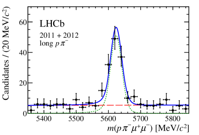
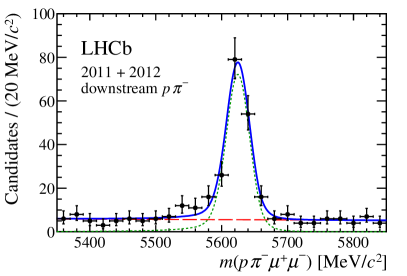
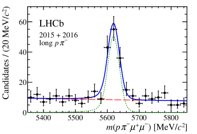
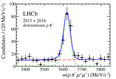
Figure 1: Distribution of $p{{\pi}^{-}}{\mu^{+}\mu^{-}}$ invariant mass for (left) long- and (right) downstream-track $p{{\pi}^{-}}$ categories in the (top) Run 1 data and (bottom) Run 2 data. The result of the fit to each sample of data is indicated by the solid blue line. The signal and background components are illustrated by the dotted green and dashed red lines, respectively.

6 Angular efficiency

The trigger, reconstruction and the selection process distort the measured angular distribution of the ${{\mathchar 28931\relax}^{0}_{b}}\!\rightarrow{\mathchar 28931\relax}{\mu^{+}\mu^{-}}$ decays. The largest distortions are found to be the result of kinematic requirements in the reconstruction, most notably due to an implicit momentum threshold applied by requiring that the muons traverse the detector and reach the muon system. The angular efficiency is parameterised in six dimensions taking into account the correlations between the different angles and the $q^{2}$-dependence of the angular efficiency.

$$\varepsilon(\vec{\Omega},{q^{2}})=\sum_{ijmnrs}c_{ijmnrs}\,L_{i}(\cos\theta)\,L_{j}(\cos\theta_{\ell})\,L_{m}(\phi_{\ell}/\pi)\,L_{n}(\cos\theta_{b})\,L_{r}(\phi_{b}/\pi)\,L_{s}({q^{2}})~{},$$ (4)

where the $L_{t}(x)$ denote a Legendre polynomial of order $t$ in variable $x$, and the $q^{2}$ range considered has been rescaled linearly between $-1$ and $+1$. The coefficients $c_{ijmnrs}$ are determined by performing a moment analysis of ${{\mathchar 28931\relax}^{0}_{b}}\!\rightarrow{\mathchar 28931\relax}{\mu^{+}\mu^{-}}$ decays simulated according to a phase-space model. The simulated decays are weighted such that they are uniformly distributed in $q^{2}$ and in the five angles, after which the angular distribution of the selected decays is proportional to the efficiency.

To achieve a good parameterisation of the efficiency, a large number of terms is required. The number of terms is reduced using an iterative approach. As a first step, the efficiency projection of each variable is parameterised independently using the sum of Legendre polynomials of up to eighth order. As a second step, correlations between pairs of angles and between individual angles and $q^{2}$ are accounted for in turn. These corrections are parameterised by sums involving pairs of polynomials that run up to sixth order in each variable. As a final step, a six-dimensional correction is applied allowing for polynomials of up to first order in the angles and $q^{2}$. Before each step, the simulated decays are corrected to remove the effects parameterised in the previous step. Small differences in the efficiency to reconstruct $p$/$\overline{p}$ and ${\pi}^{+}$/${\pi}^{-}$ are neglected.

The angular efficiency model is cross-checked in data using ${{\mathchar 28931\relax}^{0}_{b}}\!\rightarrow{{J\mskip-3.0mu/\mskip-2.0mu\psi\mskip 2.0mu}}{\mathchar 28931\relax}$ and ${{B}^{0}}\!\rightarrow{{J\mskip-3.0mu/\mskip-2.0mu\psi\mskip 2.0mu}}{{K}^{0}_{\mathrm{\scriptscriptstyle S}}}$ decays, with ${{J\mskip-3.0mu/\mskip-2.0mu\psi\mskip 2.0mu}}\!\rightarrow{\mu^{+}\mu^{-}}$. These decays have a similar topology to the ${{\mathchar 28931\relax}^{0}_{b}}\!\rightarrow{\mathchar 28931\relax}{\mu^{+}\mu^{-}}$ decay and well known angular distributions. For the ${{B}^{0}}\!\rightarrow{{J\mskip-3.0mu/\mskip-2.0mu\psi\mskip 2.0mu}}{{K}^{0}_{\mathrm{\scriptscriptstyle S}}}$ decay, where the ${K}^{0}_{\mathrm{\scriptscriptstyle S}}$ decays to ${\pi}^{+}$ ${\pi}^{-}$, the parameter $K_{1}$ is one-half and the remaining observables are equal to zero. The angular distribution of the ${{\mathchar 28931\relax}^{0}_{b}}\!\rightarrow{{J\mskip-3.0mu/\mskip-2.0mu\psi\mskip 2.0mu}}{\mathchar 28931\relax}$ decay is compatible with the measurements in Refs. [34, 35, 36].

7 Results

The angular observables are obtained using a moment analysis of the angular distribution, weighting candidates as described in Sec. 6 to account for their detection efficiency. Background is subtracted using weights obtained from the sPlot technique from the fits described in Sec. 5. The weights used to correct for the efficiency and subtract the background are determined separately for each data-taking period and for the long-track and downstream-track $p{{\pi}^{-}}$ categories. The $K_{i}$ parameters are then determined from a data set that combines the two reconstruction categories. As the polarisation of the ${\mathchar 28931\relax}^{0}_{b}$ baryons at production may vary with centre-of-mass energy between the Run 1 data, collected at $\sqrt{s}=7$ and 8$\mathrm{\,Te\kern-1.00006ptV}$, and the Run 2 data, collected at $\sqrt{s}=13\mathrm{\,Te\kern-1.00006ptV}$, these two data sets are initially treated independently. The results for the two data-taking periods are given in Appendix C. The statistical uncertainties on the various $K_{i}$ parameters are determined using a bootstrapping technique [37]. In each step of the bootstrap, the process of subtracting the background and the weighting of the candidates is repeated.

A $\chi^{2}$ comparison of the results from the two data-taking periods, taking into account the correlations between the observables, yields a $\chi^{2}$ of 35.0 with 33 degrees of freedom. This indicates an excellent agreement between the two data sets and suggests that the production polarisation is consistent for the centre-of-mass energies studied. The Run 1 and Run 2 data samples are therefore combined and the observables are determined on the combined sample. The results are given in Table 1. The correlation between the angular observables is presented in Appendix D. Figure 2 shows the one-dimensional angular projections of $\cos\theta_{\ell}$, $\cos\theta_{b}$, $\cos\theta$, $\phi_{\ell}$ and $\phi_{b}$ for the background-subtracted candidates. The data are described well by the product of the angular distributions obtained from the moment analysis and the efficiency model.

Figure 3 compares the measured observables with their corresponding SM predictions, obtained from the EOS software [38] using the values of the ${\mathchar 28931\relax}^{0}_{b}$ production polarisation measured in Ref. [34]. The values of the observables $K_{11}$ to $K_{34}$ are consistent with zero. This is expected from measurements of the angular distribution of the decay ${{\mathchar 28931\relax}^{0}_{b}}\!\rightarrow{{J\mskip-3.0mu/\mskip-2.0mu\psi\mskip 2.0mu}}{\mathchar 28931\relax}$ by CMS [36] and LHCb [34], which indicate that the production polarisation of ${\mathchar 28931\relax}^{0}_{b}$ baryons is small in $pp$ collisions at 7 and 8$\mathrm{\,Te\kern-1.00006ptV}$. The measurements are consistent with the SM predictions for $K_{1}$ to $K_{10}$. The largest discrepancy is seen in $K_{6}$, which is 2.6 standard deviations from the SM prediction. The angular observables result in an angular distribution that is not positive for all values of the angles. To obtain a physical angular distribution, $K_{6}$ has to move closer to its SM value. The measured $K_{i}$ values are also consistent with the values predicted by new physics scenarios favoured by global fits to data from $b$ to $s$ quark transitions [3, 4, 5, 6, 7]. These new physics scenarios result in only a small change of $K_{1}$ to $K_{10}$ in the low-recoil region.

The $K_{i}$ observables can be combined to determine the angular asymmetries

$$\begin{split}A^{\ell}_{\mathrm{FB}}=\tfrac{3}{2}K_{3}&=-0.39\pm 0.04\,\pm 0.01~{},\\ A^{h}_{\mathrm{FB}}=K_{4}+\tfrac{1}{2}K_{5}&=-0.30\pm 0.05\,\pm 0.02~{},\\ A^{\ell h}_{\mathrm{FB}}=\tfrac{3}{4}K_{6}&=+0.25\pm 0.04\,\pm 0.01~{},\end{split}$$

where the first uncertainties are statistical and the second are the systematic uncertainties that are discussed in the following section. The forward-backward asymmetries $A^{\ell}_{\mathrm{FB}}$ and $A^{h}_{\mathrm{FB}}$ are in good agreement with the SM predictions. The asymmetry $A^{\ell h}_{\mathrm{FB}}$, which is proportional to $K_{6}$, is 2.6 standard deviations from its SM prediction. The value of $A^{h}_{\mathrm{FB}}$ is consistent with that measured in Ref. [10]. The value of $A^{\ell}_{\mathrm{FB}}$ is not comparable due to an inconsistency in the definition of $\theta_{\ell}$ in that reference.

Table 1: Angular observables combining the results of the moments obtained from Run 1 and Run 2 data, as well as candidates reconstructed in the long- and downstream-track ${p}{{\pi}^{-}}$ categories. The first and second uncertainties are statistical and systematic, respectively.

Obs.	Value	Obs.	Value
$K_{1}$	$\phantom{+}0.346\pm 0.020\pm 0.004$	$K_{18}$	$-0.108\pm 0.058\pm 0.008$
$K_{2}$	$\phantom{+}0.308\pm 0.040\pm 0.008$	$K_{19}$	$-0.151\pm 0.122\pm 0.022$
$K_{3}$	$-0.261\pm 0.029\pm 0.006$	$K_{20}$	$-0.116\pm 0.056\pm 0.008$
$K_{4}$	$-0.176\pm 0.046\pm 0.016$	$K_{21}$	$-0.041\pm 0.105\pm 0.020$
$K_{5}$	$-0.251\pm 0.081\pm 0.016$	$K_{22}$	$-0.014\pm 0.045\pm 0.007$
$K_{6}$	$\phantom{+}0.329\pm 0.055\pm 0.012$	$K_{23}$	$-0.024\pm 0.077\pm 0.012$
$K_{7}$	$-0.015\pm 0.084\pm 0.013$	$K_{24}$	$\phantom{+}0.005\pm 0.033\pm 0.005$
$K_{8}$	$-0.099\pm 0.037\pm 0.012$	$K_{25}$	$-0.226\pm 0.176\pm 0.030$
$K_{9}$	$\phantom{+}0.005\pm 0.084\pm 0.012$	$K_{26}$	$\phantom{+}0.140\pm 0.074\pm 0.014$
$K_{10}$	$-0.045\pm 0.037\pm 0.006$	$K_{27}$	$\phantom{+}0.016\pm 0.140\pm 0.025$
$K_{11}$	$-0.007\pm 0.043\pm 0.009$	$K_{28}$	$\phantom{+}0.032\pm 0.058\pm 0.009$
$K_{12}$	$-0.009\pm 0.063\pm 0.014$	$K_{29}$	$-0.127\pm 0.097\pm 0.016$
$K_{13}$	$\phantom{+}0.024\pm 0.045\pm 0.010$	$K_{30}$	$\phantom{+}0.011\pm 0.061\pm 0.011$
$K_{14}$	$\phantom{+}0.010\pm 0.082\pm 0.013$	$K_{31}$	$\phantom{+}0.180\pm 0.094\pm 0.015$
$K_{15}$	$\phantom{+}0.158\pm 0.117\pm 0.027$	$K_{32}$	$-0.009\pm 0.055\pm 0.008$
$K_{16}$	$\phantom{+}0.050\pm 0.084\pm 0.023$	$K_{33}$	$\phantom{+}0.022\pm 0.060\pm 0.009$
$K_{17}$	$-0.000\pm 0.120\pm 0.022$	$K_{34}$	$\phantom{+}0.060\pm 0.058\pm 0.009$

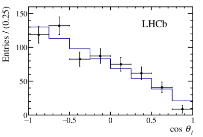
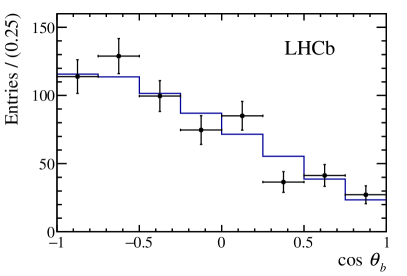
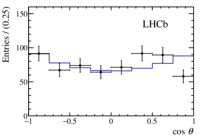
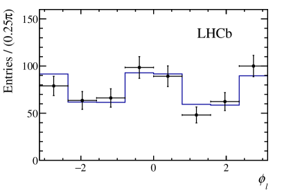
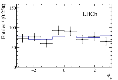
Figure 2: One-dimensional projections of the angular distributions of the candidates (black points), combining Run 1 and Run 2 data, as well as candidates reconstructed in the long- and downstream-track $p{{\pi}^{-}}$ categories. The background is subtracted from the data but no efficiency correction is applied. The projection of each angular distribution obtained from the moment analysis multiplied by the efficiency distribution is superimposed. The large variation in $\phi_{\ell}$ is primarily due to the angular acceptance.

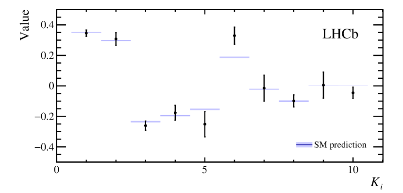
Figure 3: Angular observables combining the results for the moments obtained from Run 1 and Run 2 data, as well as candidates reconstructed in the long- and downstream-track ${p}{{\pi}^{-}}$ categories. The blue line represents the SM predictions obtained using the EOS software. The thickness of the light-blue band represents the uncertainty on the SM predictions.

8 Systematic uncertainties

The angular observables may be sensitive to systematic effects arising from imperfect modelling of either the angular efficiency or the $m(p{{\pi}^{-}}{\mu^{+}\mu^{-}})$ distribution. Where possible, systematic uncertainties are estimated using pseudoexperiments. These are generated from a systematically varied model and the observables are then estimated using the nominal analysis, neglecting the variation in the generation. The sources of systematic uncertainty considered are listed in Table 2. In general, systematic uncertainties are found to be small compared to the statistical uncertainties on the measurements.

The largest systematic uncertainties in modelling the angular efficiency are from the size of the simulated data samples and the order of the Legendre polynomials used to parameterise the efficiency. The former is determined by bootstrapping the simulated sample and re-evaluating the model. The latter is estimated by increasing the order of polynomials used in the efficiency parameterisation by up to two orders. By default, the efficiency model is chosen to have the minimum number of terms needed to get a good description of both the simulated and the data control samples. Increasing further the number of terms results in an overfitting of statistical fluctuations in the simulated data used to determine the efficiency model (due to the limited size of the simulated data set).

A systematic uncertainty due to the modelling of the data by the simulation is estimated by varying the tracking and muon identification efficiencies, and by applying an additional correction to the $p_{\mathrm{T}}$ and $\eta$ spectra of the ${\mathchar 28931\relax}^{0}_{b}$ baryons.

The impact of neglecting angular resolution when determining the angular observables is estimated by smearing pseudoexperiments according to the resolution determined using simulated data. The angular resolution is poorest for $\theta$, $\theta_{b}$ and $\phi_{b}$ in the downstream $p{{\pi}^{-}}$ category, at around 90$\mathrm{\,mrad}$ for $\theta$ and $\theta_{b}$ and 150$\mathrm{\,mrad}$ for $\phi_{b}$.

In the calculation of the angular basis, the crossing angle of the LHC beams is neglected. The impact of this is estimated by generating pseudoexperiments with the correct crossing angle and neglecting this when the angular observables are determined.

The systematic uncertainty due to modelling the shape of the signal mass distribution is small. The main contribution to this uncertainty comes from the modelling of the tails of the signal mass distribution. The factorisation of the mass model and the angular distribution, which is a requirement of the sPlot technique, is also tested and results in a negligible systematic uncertainty.

Table 2: Sources of systematic uncertainty on the $K_{i}$ angular observables, together with the mean and the range of uncertainty values assigned to the 34 $K_{i}$ parameters in each case. The variation of each source of systematic uncertainty between the different observables depends on the structure of the weighting functions used to extract the observable and its correlation with the angular efficiency.

Source	Uncertainty [$10^{-3}$]
	Range among $K_{i}$	Mean
Simulated sample size	3–22	9
Efficiency parameterisation	1–13	4
Data-simulation differences	2–16	6
Angular resolution	1–11	4
Beam crossing angle	1–8	4
Signal mass model	1–4	2

9 Summary

An analysis of the angular distribution of the decay ${{\mathchar 28931\relax}^{0}_{b}}\!\rightarrow{\mathchar 28931\relax}{\mu^{+}\mu^{-}}$ in the dimuon invariant mass squared range $15<{q^{2}}<20\mathrm{\,Ge\kern-1.00006ptV}^{2}/c^{4}$ is reported. Using data collected with the LHCb detector between 2011 and 2016, the full basis of angular observables is measured for the first time. From the measured observables, the lepton-side, hadron-side and combined forward-backward asymmetries of the decay are determined to be

$$\begin{split}A^{\ell}_{\mathrm{FB}}&=-0.39\pm 0.04\mathrm{\,(stat)}\,\pm 0.01\mathrm{\,(syst)}~{},\\ A^{h}_{\mathrm{FB}}&=-0.30\pm 0.05\mathrm{\,(stat)}\,\pm 0.02\mathrm{\,(syst)}~{},\\ A^{\ell h}_{\mathrm{FB}}&=+0.25\pm 0.04\mathrm{\,(stat)}\,\pm 0.01\mathrm{\,(syst)}~{}.\end{split}$$

The results presented here supersede the results for angular observables in Ref. [10] (see discussion in Sec. 7). The measured angular observables are compatible with the SM predictions obtained using the EOS software [38], where the ${\mathchar 28931\relax}^{0}_{b}$ production polarisation is set to the value obtained by the LHCb collaboration in $pp$ collisions at a centre-of-mass energy of $7$ TeV [34].

Appendix A Angular basis

The angular distribution of the decay ${{\mathchar 28931\relax}^{0}_{b}}\!\rightarrow{\mathchar 28931\relax}{\mu^{+}\mu^{-}}$ is described by five angles, $\theta$, $\theta_{\ell}$, $\phi_{\ell}$, $\theta_{b}$ and $\phi_{b}$ defined with respect to the normal-vector

$$\hat{n}=\frac{\vec{p}_{\rm beam}^{\,\{{\rm lab}\}}\times\vec{p}_{{{\mathchar 28931\relax}^{0}_{b}}}^{\,\{{\rm lab}\}}}{|\vec{p}_{\rm beam}^{\,\{{\rm lab}\}}\times\vec{p}_{{{\mathchar 28931\relax}^{0}_{b}}}^{\,\{{\rm lab}\}}|}~{},$$ (5)

where $\hat{p}=\vec{p}/|\vec{p}|$ and the parentheses refer to the rest frame the momentum is measured in. The angle $\theta$ is defined by the angle between $\hat{n}$ and the $\mathchar 28931\relax$ baryon momentum in the ${\mathchar 28931\relax}^{0}_{b}$ baryon rest frame, i.e.

$$\cos\theta=\hat{n}\cdot\hat{p}_{{\mathchar 28931\relax}}^{\{{{\mathchar 28931\relax}^{0}_{b}}\}}~{}.$$ (6)

The decay of the $\mathchar 28931\relax$ baryon and the dimuon system can be described by coordinate systems with $\hat{z}_{b}=\hat{p}_{{\mathchar 28931\relax}}^{\{{{\mathchar 28931\relax}^{0}_{b}}\}}$ and $\hat{z}_{\ell}=\hat{p}_{{\mu^{+}\mu^{-}}}^{\{{{\mathchar 28931\relax}^{0}_{b}}\}}$, $\hat{y}_{b,\ell}=\hat{n}\times\hat{z}_{b,\ell}$ and $\hat{x}_{b,\ell}=\hat{z}_{b,\ell}\times\hat{y}_{b,\ell}$. The angles $\theta_{b}$ and $\phi_{b}$ ($\theta_{\ell}$ and $\phi_{\ell}$) are the polar and azimuthal angle of the proton ($\mu^{+}$) in the $\mathchar 28931\relax$ baryon (dimuon) rest frame. The angles are defined by

$$\begin{split}\cos\theta_{b,\ell}&=\hat{z}_{b,\ell}\cdot\hat{p}_{b,\ell}~{},~{}\cos\phi_{b,\ell}=\hat{x}_{b,\ell}\cdot\hat{p}_{\perp b,\ell}~{},~{}\sin\phi_{b,\ell}=\hat{y}_{b,\ell}\cdot\hat{p}_{\perp b,\ell}~{},\end{split}$$ (7)

where $\hat{p}_{b}$ $(\hat{p}_{\ell})$ is the direction of the proton ($\mu^{+}$) and $\hat{p}_{\perp b}$ $(\hat{p}_{\perp\ell})$ is a unit vector corresponding to the component perpendicular to the $\hat{z}_{b}$ $(\hat{z}_{\ell})$ axis. For the ${\kern 1.00006pt\overline{\kern-1.00006pt\mathchar 28931\relax}}{}^{0}_{b}$ decay, the angular variables are transformed such that $\theta_{\ell}\rightarrow\pi-\theta_{\ell}$, $\phi_{\ell}\rightarrow\pi-\phi_{\ell}$ and $\phi_{b}\rightarrow-\phi_{b}$. This ensures that, in the absence of $C\!P$ violating effects, the $K_{i}$ observables are the same for ${\mathchar 28931\relax}^{0}_{b}$ and ${\kern 1.00006pt\overline{\kern-1.00006pt\mathchar 28931\relax}}{}^{0}_{b}$ decays.

Appendix B Angular distribution and weighting functions

The full form of the angular distribution of the decay ${{\mathchar 28931\relax}^{0}_{b}}\!\rightarrow{\mathchar 28931\relax}{\mu^{+}\mu^{-}}$ is given by

$$\frac{\mathrm{d}^{5}\Gamma}{\mathrm{d}\vec{\Omega}}=\frac{3}{32\pi^{2}}\Big{(} \left(K_{1}\sin^{2}\theta_{\ell}+K_{2}\cos^{2}\theta_{\ell}+K_{3}\cos\theta_{\ell}\right)+$$ (8)

$$\left(K_{4}\sin^{2}\theta_{\ell}+K_{5}\cos^{2}\theta_{\ell}+K_{6}\cos\theta_{\ell}\right)\cos\theta_{b}+$$

$$\left(K_{7}\sin\theta_{\ell}\cos\theta_{\ell}+K_{8}\sin\theta_{\ell}\right)\sin\theta_{b}\cos\left(\phi_{b}+\phi_{\ell}\right)+$$

$$\left(K_{9}\sin\theta_{\ell}\cos\theta_{\ell}+K_{10}\sin\theta_{\ell}\right)\sin\theta_{b}\sin\left(\phi_{b}+\phi_{\ell}\right)+$$

$$\left(K_{11}\sin^{2}\theta_{\ell}+K_{12}\cos^{2}\theta_{\ell}+K_{13}\cos\theta_{\ell}\right)\cos\theta+$$

$$\left(K_{14}\sin^{2}\theta_{\ell}+K_{15}\cos^{2}\theta_{\ell}+K_{16}\cos\theta_{\ell}\right)\cos\theta_{b}\cos\theta+$$

$$\left(K_{17}\sin\theta_{\ell}\cos\theta_{\ell}+K_{18}\sin\theta_{\ell}\right)\sin\theta_{b}\cos\left(\phi_{b}+\phi_{\ell}\right)\cos\theta+$$

$$\left(K_{19}\sin\theta_{\ell}\cos\theta_{\ell}+K_{20}\sin\theta_{\ell}\right)\sin\theta_{b}\sin\left(\phi_{b}+\phi_{\ell}\right)\cos\theta+$$

$$\left(K_{21}\cos\theta_{\ell}\sin\theta_{\ell}+K_{22}\sin\theta_{\ell}\right)\sin\phi_{\ell}\sin\theta+$$

$$\left(K_{23}\cos\theta_{\ell}\sin\theta_{\ell}+K_{24}\sin\theta_{\ell}\right)\cos\phi_{\ell}\sin\theta+$$

$$\left(K_{25}\cos\theta_{\ell}\sin\theta_{\ell}+K_{26}\sin\theta_{\ell}\right)\sin\phi_{\ell}\cos\theta_{b}\sin\theta+$$

$$\left(K_{27}\cos\theta_{\ell}\sin\theta_{\ell}+K_{28}\sin\theta_{\ell}\right)\cos\phi_{\ell}\cos\theta_{b}\sin\theta+$$

$$\left(K_{29}\cos^{2}\theta_{\ell}+K_{30}\sin^{2}\theta_{\ell}\right)\sin\theta_{b}\sin\phi_{b}\sin\theta+$$

$$\left(K_{31}\cos^{2}\theta_{\ell}+K_{32}\sin^{2}\theta_{\ell}\right)\sin\theta_{b}\cos\phi_{b}\sin\theta+$$

$$\left(K_{33}\sin^{2}\theta_{\ell}\right)\sin\theta_{b}\cos\left(2\phi_{\ell}+\phi_{b}\right)\sin\theta+$$

$$\left(K_{34}\sin^{2}\theta_{\ell}\right)\sin\theta_{b}\sin\left(2\phi_{\ell}+\phi_{b}\right)\sin\theta\Big{)}~{}.$$

The individual $K_{i}$ parameters can be determined using a moment analysis of the angular distribution with the weighting functions

$$g_{1}(\vec{\Omega})= \tfrac{1}{4}(3-5\cos^{2}\theta_{\ell})~{}, g_{6}(\vec{\Omega})~{}=3\cos\theta_{\ell}\cos\theta_{b}~{},$$ (9)

$$g_{2}(\vec{\Omega})= \tfrac{1}{2}(5\cos^{2}\theta_{\ell}-1)~{}, g_{7}(\vec{\Omega})~{}=\tfrac{15}{2}\cos\theta_{\ell}\sin\theta_{\ell}\sin\theta_{b}\cos(\phi_{\ell}+\phi_{b})~{},$$

$$g_{3}(\vec{\Omega})= \cos\theta_{\ell}~{}, g_{8}(\vec{\Omega})~{}=\tfrac{3}{2}\sin\theta_{\ell}\sin\theta_{b}\cos(\phi_{\ell}+\phi_{b})~{},$$

$$g_{4}(\vec{\Omega})= \tfrac{3}{4}(3-5\cos^{2}\theta_{\ell})\cos\theta_{b}~{}, g_{9}(\vec{\Omega})~{}=\tfrac{15}{2}\cos\theta_{\ell}\sin\theta_{\ell}\sin\theta_{b}\sin(\phi_{\ell}+\phi_{b})~{},$$

$$g_{5}(\vec{\Omega})= \tfrac{3}{2}(5\cos^{2}\theta_{\ell}-1)\cos\theta_{b}~{}, g_{10}(\vec{\Omega})=\tfrac{3}{2}\sin\theta_{\ell}\sin\theta_{b}\sin(\phi_{\ell}+\phi_{b})~{},$$

from Ref. [15] and the weighting functions

$$g_{11}(\vec{\Omega})= \tfrac{3}{4}(3-5\cos^{2}\theta_{\ell})\cos\theta~{}, g_{23}(\vec{\Omega})=\tfrac{15}{2}\cos\theta_{\ell}\sin\theta_{\ell}\sin\theta\cos\phi_{\ell}~{},$$ (10)

$$g_{12}(\vec{\Omega})= \tfrac{3}{2}(5\cos^{2}\theta_{\ell}-1)\cos\theta~{}, g_{24}(\vec{\Omega})=\tfrac{3}{2}\sin\theta\sin\theta_{\ell}\cos\phi_{\ell}~{},$$

$$g_{13}(\vec{\Omega})= 3\cos\theta_{\ell}\cos\theta~{}, g_{25}(\vec{\Omega})=\tfrac{45}{2}\cos\theta_{\ell}\sin\theta_{\ell}\cos\theta_{b}\sin\theta\sin\phi_{\ell}~{},$$

$$g_{14}(\vec{\Omega})= \tfrac{9}{4}(3-5\cos^{2}\theta_{\ell})\cos\theta_{b}\cos\theta~{}, g_{26}(\vec{\Omega})=\tfrac{9}{2}\sin\theta\sin\theta_{\ell}\cos\theta_{b}\sin\phi_{\ell}~{},$$

$$g_{15}(\vec{\Omega})= \tfrac{9}{2}(5\cos^{2}\theta_{\ell}-1)\cos\theta_{b}\cos\theta~{}, g_{27}(\vec{\Omega})=\tfrac{45}{2}\cos\theta_{\ell}\sin\theta_{\ell}\cos\theta_{b}\sin\theta\cos\phi_{\ell}~{},$$

$$g_{16}(\vec{\Omega})= 9\cos\theta\cos\theta_{\ell}\cos\theta_{b}~{}, g_{28}(\vec{\Omega})=\tfrac{9}{2}\sin\theta\sin\theta_{\ell}\cos\theta_{b}\cos\phi_{\ell}~{},$$

$$g_{17}(\vec{\Omega})= \tfrac{45}{2}\cos\theta_{\ell}\sin\theta_{\ell}\sin\theta_{b}\cos\theta\cos(\phi_{\ell}+\phi_{b})~{}, g_{29}(\vec{\Omega})=\tfrac{9}{4}(5\cos^{2}\theta_{\ell}-1)\sin\theta_{b}\sin\theta\sin\phi_{b}~{},$$

$$g_{18}(\vec{\Omega})= \tfrac{9}{2}\sin\theta_{\ell}\sin\theta_{b}\cos\theta\cos(\phi_{\ell}+\phi_{b})~{}, g_{30}(\vec{\Omega})=\tfrac{9}{8}(3-5\cos^{2}\theta_{\ell})\sin\theta_{b}\sin\theta\sin\phi_{b}~{},$$

$$g_{19}(\vec{\Omega})= \tfrac{45}{2}\cos\theta_{\ell}\sin\theta_{\ell}\sin\theta_{b}\cos\theta\sin(\phi_{\ell}+\phi_{b})~{}, g_{31}(\vec{\Omega})=\tfrac{9}{4}(5\cos^{2}\theta_{\ell}-1)\sin\theta_{b}\sin\theta\cos\phi_{b}~{},$$

$$g_{20}(\vec{\Omega})= \tfrac{9}{2}\sin\theta_{\ell}\sin\theta_{b}\cos\theta\sin(\phi_{\ell}+\phi_{b})~{}, g_{32}(\vec{\Omega})=\tfrac{9}{8}(3-5\cos^{2}\theta_{\ell})\sin\theta_{b}\sin\theta\cos\phi_{b}~{},$$

$$g_{21}(\vec{\Omega})= \tfrac{15}{2}\cos\theta_{\ell}\sin\theta_{\ell}\sin\theta\sin\phi_{\ell}~{}, g_{33}(\vec{\Omega})=\tfrac{9}{4}\sin\theta_{b}\sin\theta\cos(2\phi_{\ell}+\phi_{b})~{},$$

$$g_{22}(\vec{\Omega})= \tfrac{3}{2}\sin\theta\sin\theta_{\ell}\sin\phi_{\ell}~{}, g_{34}(\vec{\Omega})=\tfrac{9}{4}\sin\theta_{b}\sin\theta\sin(2\phi_{\ell}+\phi_{b})~{},$$

from Ref. [11].

Appendix C Results separated by data-taking period

Tables 3 and 4 show the values of the observables for each of the two data-taking periods. Table 3 shows the values of the observables combining the 2011 data, collected at $\sqrt{s}=7\mathrm{\,Te\kern-1.00006ptV}$, and the 2012 data, collected at $\sqrt{s}=8\mathrm{\,Te\kern-1.00006ptV}$. Table 4 shows the values of the observables in the Run 2 data, collected at $\sqrt{s}=13\mathrm{\,Te\kern-1.00006ptV}$.

Table 3: Measured values for the angular observables from the Run 1 data combining the results of the moments obtained from the candidates reconstructed in the long- and downstream-track ${p}{{\pi}^{-}}$ categories. The first and second uncertainties are statistical and systematic, respectively.

Obs.	Value	Obs.	Value
$K_{1}$	$\phantom{+}0.376\pm 0.029\pm 0.006$	$K_{18}$	$-0.081\pm 0.081\pm 0.015$
$K_{2}$	$\phantom{+}0.248\pm 0.057\pm 0.012$	$K_{19}$	$-0.023\pm 0.165\pm 0.031$
$K_{3}$	$-0.241\pm 0.041\pm 0.008$	$K_{20}$	$-0.156\pm 0.078\pm 0.019$
$K_{4}$	$-0.212\pm 0.070\pm 0.013$	$K_{21}$	$-0.050\pm 0.150\pm 0.032$
$K_{5}$	$-0.123\pm 0.117\pm 0.020$	$K_{22}$	$\phantom{+}0.032\pm 0.064\pm 0.014$
$K_{6}$	$\phantom{+}0.247\pm 0.079\pm 0.017$	$K_{23}$	$\phantom{+}0.038\pm 0.104\pm 0.018$
$K_{7}$	$-0.027\pm 0.124\pm 0.022$	$K_{24}$	$\phantom{+}0.004\pm 0.047\pm 0.008$
$K_{8}$	$-0.081\pm 0.054\pm 0.010$	$K_{25}$	$-0.107\pm 0.254\pm 0.046$
$K_{9}$	$-0.123\pm 0.115\pm 0.018$	$K_{26}$	$\phantom{+}0.130\pm 0.106\pm 0.024$
$K_{10}$	$\phantom{+}0.021\pm 0.051\pm 0.009$	$K_{27}$	$-0.200\pm 0.190\pm 0.035$
$K_{11}$	$-0.030\pm 0.062\pm 0.014$	$K_{28}$	$\phantom{+}0.058\pm 0.084\pm 0.015$
$K_{12}$	$-0.114\pm 0.092\pm 0.022$	$K_{29}$	$-0.172\pm 0.142\pm 0.027$
$K_{13}$	$\phantom{+}0.059\pm 0.064\pm 0.016$	$K_{30}$	$-0.060\pm 0.088\pm 0.014$
$K_{14}$	$\phantom{+}0.122\pm 0.126\pm 0.026$	$K_{31}$	$\phantom{+}0.252\pm 0.126\pm 0.022$
$K_{15}$	$\phantom{+}0.247\pm 0.171\pm 0.042$	$K_{32}$	$-0.074\pm 0.075\pm 0.011$
$K_{16}$	$-0.193\pm 0.116\pm 0.029$	$K_{33}$	$-0.010\pm 0.081\pm 0.014$
$K_{17}$	$-0.119\pm 0.178\pm 0.033$	$K_{34}$	$\phantom{+}0.140\pm 0.088\pm 0.012$

Table 4: Measured values for the angular observables from the Run 2 data combining the results of the moments obtained from the candidates reconstructed in the long- and downstream-track ${p}{{\pi}^{-}}$ categories. The first and second uncertainties are statistical and systematic, respectively.

Obs.	Value	Obs.	Value
$K_{1}$	$\phantom{+}0.318\pm 0.028\pm 0.007$	$K_{18}$	$-0.134\pm 0.081\pm 0.014$
$K_{2}$	$\phantom{+}0.364\pm 0.056\pm 0.013$	$K_{19}$	$-0.273\pm 0.178\pm 0.040$
$K_{3}$	$-0.279\pm 0.042\pm 0.010$	$K_{20}$	$-0.078\pm 0.082\pm 0.017$
$K_{4}$	$-0.143\pm 0.063\pm 0.012$	$K_{21}$	$-0.033\pm 0.142\pm 0.023$
$K_{5}$	$-0.372\pm 0.113\pm 0.024$	$K_{22}$	$-0.058\pm 0.062\pm 0.008$
$K_{6}$	$\phantom{+}0.407\pm 0.076\pm 0.017$	$K_{23}$	$-0.082\pm 0.111\pm 0.018$
$K_{7}$	$-0.004\pm 0.114\pm 0.018$	$K_{24}$	$\phantom{+}0.005\pm 0.046\pm 0.008$
$K_{8}$	$-0.116\pm 0.051\pm 0.011$	$K_{25}$	$-0.339\pm 0.243\pm 0.042$
$K_{9}$	$\phantom{+}0.126\pm 0.124\pm 0.017$	$K_{26}$	$\phantom{+}0.150\pm 0.101\pm 0.017$
$K_{10}$	$-0.108\pm 0.054\pm 0.008$	$K_{27}$	$\phantom{+}0.221\pm 0.203\pm 0.036$
$K_{11}$	$\phantom{+}0.014\pm 0.060\pm 0.009$	$K_{28}$	$\phantom{+}0.008\pm 0.083\pm 0.015$
$K_{12}$	$\phantom{+}0.091\pm 0.085\pm 0.023$	$K_{29}$	$-0.085\pm 0.135\pm 0.025$
$K_{13}$	$-0.009\pm 0.063\pm 0.016$	$K_{30}$	$\phantom{+}0.079\pm 0.084\pm 0.014$
$K_{14}$	$-0.096\pm 0.105\pm 0.019$	$K_{31}$	$\phantom{+}0.113\pm 0.140\pm 0.021$
$K_{15}$	$\phantom{+}0.073\pm 0.159\pm 0.046$	$K_{32}$	$\phantom{+}0.053\pm 0.080\pm 0.012$
$K_{16}$	$\phantom{+}0.280\pm 0.120\pm 0.034$	$K_{33}$	$\phantom{+}0.052\pm 0.088\pm 0.011$
$K_{17}$	$\phantom{+}0.112\pm 0.166\pm 0.033$	$K_{34}$	$-0.015\pm 0.079\pm 0.012$

Appendix D Correlation matrices

Figures 4 and 5 shows the statistical correlation between the angular observables determined using bootstrapped samples. The correlation coefficients are typically small but can be as large as 30–40% between pairs of observables. The observables $K_{1}$ and $K_{2}$ are fully anticorrelated due to the normalisation of the observables, which requires $2K_{1}+K_{2}=1$. The correlation matrices in numerical form are attached as supplementary material to this article.

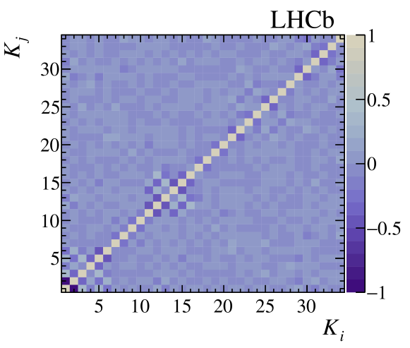
Figure 4: Correlation coefficients between observables for the combined Run 1 and Run 2 data. The correlations are estimated using bootstrapped samples.

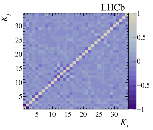
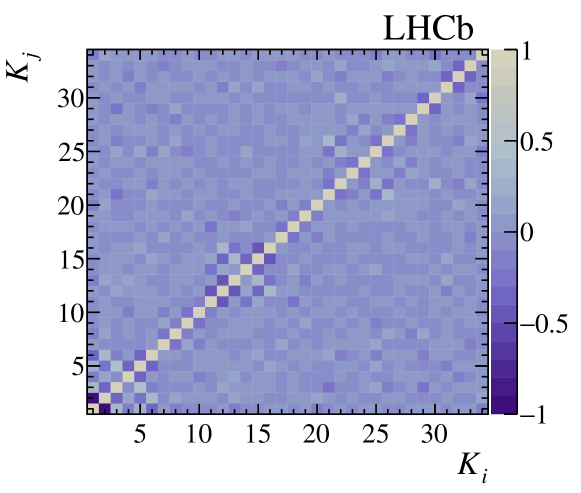
Figure 5: Correlation coefficients between the observables (top) in the Run 1 data and (bottom) in the Run 2 data. The correlations are estimated using bootstrapped samples.

LHCb collaboration

R. Aaij²⁷, B. Adeva⁴¹, M. Adinolfi⁴⁸, C.A. Aidala⁷³, Z. Ajaltouni⁵, S. Akar⁵⁹, P. Albicocco¹⁸, J. Albrecht¹⁰, F. Alessio⁴², M. Alexander⁵³, A. Alfonso Albero⁴⁰, S. Ali²⁷, G. Alkhazov³³, P. Alvarez Cartelle⁵⁵, A.A. Alves Jr⁴¹, S. Amato², S. Amerio²³, Y. Amhis⁷, L. An³, L. Anderlini¹⁷, G. Andreassi⁴³, M. Andreotti^16,g, J.E. Andrews⁶⁰, R.B. Appleby⁵⁶, F. Archilli²⁷, P. d’Argent¹², J. Arnau Romeu⁶, A. Artamonov³⁹, M. Artuso⁶¹, K. Arzymatov³⁷, E. Aslanides⁶, M. Atzeni⁴⁴, B. Audurier²², S. Bachmann¹², J.J. Back⁵⁰, S. Baker⁵⁵, V. Balagura^7,b, W. Baldini¹⁶, A. Baranov³⁷, R.J. Barlow⁵⁶, S. Barsuk⁷, W. Barter⁵⁶, F. Baryshnikov⁷⁰, V. Batozskaya³¹, B. Batsukh⁶¹, V. Battista⁴³, A. Bay⁴³, J. Beddow⁵³, F. Bedeschi²⁴, I. Bediaga¹, A. Beiter⁶¹, L.J. Bel²⁷, S. Belin²², N. Beliy⁶³, V. Bellee⁴³, N. Belloli^20,i, K. Belous³⁹, I. Belyaev^34,42, E. Ben-Haim⁸, G. Bencivenni¹⁸, S. Benson²⁷, S. Beranek⁹, A. Berezhnoy³⁵, R. Bernet⁴⁴, D. Berninghoff¹², E. Bertholet⁸, A. Bertolin²³, C. Betancourt⁴⁴, F. Betti^15,42, M.O. Bettler⁴⁹, M. van Beuzekom²⁷, Ia. Bezshyiko⁴⁴, S. Bhasin⁴⁸, J. Bhom²⁹, S. Bifani⁴⁷, P. Billoir⁸, A. Birnkraut¹⁰, A. Bizzeti^17,u, M. Bjørn⁵⁷, M.P. Blago⁴², T. Blake⁵⁰, F. Blanc⁴³, S. Blusk⁶¹, D. Bobulska⁵³, V. Bocci²⁶, O. Boente Garcia⁴¹, T. Boettcher⁵⁸, A. Bondar^38,w, N. Bondar³³, S. Borghi^56,42, M. Borisyak³⁷, M. Borsato⁴¹, F. Bossu⁷, M. Boubdir⁹, T.J.V. Bowcock⁵⁴, C. Bozzi^16,42, S. Braun¹², M. Brodski⁴², J. Brodzicka²⁹, A. Brossa Gonzalo⁵⁰, D. Brundu²², E. Buchanan⁴⁸, A. Buonaura⁴⁴, C. Burr⁵⁶, A. Bursche²², J. Buytaert⁴², W. Byczynski⁴², S. Cadeddu²², H. Cai⁶⁴, R. Calabrese^16,g, R. Calladine⁴⁷, M. Calvi^20,i, M. Calvo Gomez^40,m, A. Camboni^40,m, P. Campana¹⁸, D.H. Campora Perez⁴², L. Capriotti⁵⁶, A. Carbone^15,e, G. Carboni²⁵, R. Cardinale^19,h, A. Cardini²², P. Carniti^20,i, L. Carson⁵², K. Carvalho Akiba², G. Casse⁵⁴, L. Cassina²⁰, M. Cattaneo⁴², G. Cavallero^19,h, R. Cenci^24,p, D. Chamont⁷, M.G. Chapman⁴⁸, M. Charles⁸, Ph. Charpentier⁴², G. Chatzikonstantinidis⁴⁷, M. Chefdeville⁴, V. Chekalina³⁷, C. Chen³, S. Chen²², S.-G. Chitic⁴², V. Chobanova⁴¹, M. Chrzaszcz⁴², A. Chubykin³³, P. Ciambrone¹⁸, X. Cid Vidal⁴¹, G. Ciezarek⁴², P.E.L. Clarke⁵², M. Clemencic⁴², H.V. Cliff⁴⁹, J. Closier⁴², V. Coco⁴², J.A.B. Coelho⁷, J. Cogan⁶, E. Cogneras⁵, L. Cojocariu³², P. Collins⁴², T. Colombo⁴², A. Comerma-Montells¹², A. Contu²², G. Coombs⁴², S. Coquereau⁴⁰, G. Corti⁴², M. Corvo^16,g, C.M. Costa Sobral⁵⁰, B. Couturier⁴², G.A. Cowan⁵², D.C. Craik⁵⁸, A. Crocombe⁵⁰, M. Cruz Torres¹, R. Currie⁵², C. D’Ambrosio⁴², F. Da Cunha Marinho², C.L. Da Silva⁷⁴, E. Dall’Occo²⁷, J. Dalseno⁴⁸, A. Danilina³⁴, A. Davis³, O. De Aguiar Francisco⁴², K. De Bruyn⁴², S. De Capua⁵⁶, M. De Cian⁴³, J.M. De Miranda¹, L. De Paula², M. De Serio^14,d, P. De Simone¹⁸, C.T. Dean⁵³, D. Decamp⁴, L. Del Buono⁸, B. Delaney⁴⁹, H.-P. Dembinski¹¹, M. Demmer¹⁰, A. Dendek³⁰, D. Derkach³⁷, O. Deschamps⁵, F. Desse⁷, F. Dettori⁵⁴, B. Dey⁶⁵, A. Di Canto⁴², P. Di Nezza¹⁸, S. Didenko⁷⁰, H. Dijkstra⁴², F. Dordei⁴², M. Dorigo^42,y, A. Dosil Suárez⁴¹, L. Douglas⁵³, A. Dovbnya⁴⁵, K. Dreimanis⁵⁴, L. Dufour²⁷, G. Dujany⁸, P. Durante⁴², J.M. Durham⁷⁴, D. Dutta⁵⁶, R. Dzhelyadin³⁹, M. Dziewiecki¹², A. Dziurda²⁹, A. Dzyuba³³, S. Easo⁵¹, U. Egede⁵⁵, V. Egorychev³⁴, S. Eidelman^38,w, S. Eisenhardt⁵², U. Eitschberger¹⁰, R. Ekelhof¹⁰, L. Eklund⁵³, S. Ely⁶¹, A. Ene³², S. Escher⁹, S. Esen²⁷, T. Evans⁵⁹, C. Everett⁵⁰, A. Falabella¹⁵, N. Farley⁴⁷, S. Farry⁵⁴, D. Fazzini^20,42,i, L. Federici²⁵, P. Fernandez Declara⁴², A. Fernandez Prieto⁴¹, F. Ferrari¹⁵, L. Ferreira Lopes⁴³, F. Ferreira Rodrigues², M. Ferro-Luzzi⁴², S. Filippov³⁶, R.A. Fini¹⁴, M. Fiorini^16,g, M. Firlej³⁰, C. Fitzpatrick⁴³, T. Fiutowski³⁰, F. Fleuret^7,b, M. Fontana^22,42, F. Fontanelli^19,h, R. Forty⁴², V. Franco Lima⁵⁴, M. Frank⁴², C. Frei⁴², J. Fu^21,q, W. Funk⁴², C. Färber⁴², M. Féo Pereira Rivello Carvalho²⁷, E. Gabriel⁵², A. Gallas Torreira⁴¹, D. Galli^15,e, S. Gallorini²³, S. Gambetta⁵², Y. Gan³, M. Gandelman², P. Gandini²¹, Y. Gao³, L.M. Garcia Martin⁷², B. Garcia Plana⁴¹, J. García Pardiñas⁴⁴, J. Garra Tico⁴⁹, L. Garrido⁴⁰, D. Gascon⁴⁰, C. Gaspar⁴², L. Gavardi¹⁰, G. Gazzoni⁵, D. Gerick¹², E. Gersabeck⁵⁶, M. Gersabeck⁵⁶, T. Gershon⁵⁰, D. Gerstel⁶, Ph. Ghez⁴, S. Gianì⁴³, V. Gibson⁴⁹, O.G. Girard⁴³, L. Giubega³², K. Gizdov⁵², V.V. Gligorov⁸, D. Golubkov³⁴, A. Golutvin^55,70, A. Gomes^1,a, I.V. Gorelov³⁵, C. Gotti^20,i, E. Govorkova²⁷, J.P. Grabowski¹², R. Graciani Diaz⁴⁰, L.A. Granado Cardoso⁴², E. Graugés⁴⁰, E. Graverini⁴⁴, G. Graziani¹⁷, A. Grecu³², R. Greim²⁷, P. Griffith²², L. Grillo⁵⁶, L. Gruber⁴², B.R. Gruberg Cazon⁵⁷, O. Grünberg⁶⁷, C. Gu³, E. Gushchin³⁶, Yu. Guz^39,42, T. Gys⁴², C. Göbel⁶², T. Hadavizadeh⁵⁷, C. Hadjivasiliou⁵, G. Haefeli⁴³, C. Haen⁴², S.C. Haines⁴⁹, B. Hamilton⁶⁰, X. Han¹², T.H. Hancock⁵⁷, S. Hansmann-Menzemer¹², N. Harnew⁵⁷, S.T. Harnew⁴⁸, T. Harrison⁵⁴, C. Hasse⁴², M. Hatch⁴², J. He⁶³, M. Hecker⁵⁵, K. Heinicke¹⁰, A. Heister¹⁰, K. Hennessy⁵⁴, L. Henry⁷², E. van Herwijnen⁴², M. Heß⁶⁷, A. Hicheur², R. Hidalgo Charman⁵⁶, D. Hill⁵⁷, M. Hilton⁵⁶, P.H. Hopchev⁴³, W. Hu⁶⁵, W. Huang⁶³, Z.C. Huard⁵⁹, W. Hulsbergen²⁷, T. Humair⁵⁵, M. Hushchyn³⁷, D. Hutchcroft⁵⁴, D. Hynds²⁷, P. Ibis¹⁰, M. Idzik³⁰, P. Ilten⁴⁷, K. Ivshin³³, R. Jacobsson⁴², J. Jalocha⁵⁷, E. Jans²⁷, A. Jawahery⁶⁰, F. Jiang³, M. John⁵⁷, D. Johnson⁴², C.R. Jones⁴⁹, C. Joram⁴², B. Jost⁴², N. Jurik⁵⁷, S. Kandybei⁴⁵, M. Karacson⁴², J.M. Kariuki⁴⁸, S. Karodia⁵³, N. Kazeev³⁷, M. Kecke¹², F. Keizer⁴⁹, M. Kelsey⁶¹, M. Kenzie⁴⁹, T. Ketel²⁸, E. Khairullin³⁷, B. Khanji¹², C. Khurewathanakul⁴³, K.E. Kim⁶¹, T. Kirn⁹, S. Klaver¹⁸, K. Klimaszewski³¹, T. Klimkovich¹¹, S. Koliiev⁴⁶, M. Kolpin¹², R. Kopecna¹², P. Koppenburg²⁷, I. Kostiuk²⁷, S. Kotriakhova³³, M. Kozeiha⁵, L. Kravchuk³⁶, M. Kreps⁵⁰, F. Kress⁵⁵, P. Krokovny^38,w, W. Krupa³⁰, W. Krzemien³¹, W. Kucewicz^29,l, M. Kucharczyk²⁹, V. Kudryavtsev^38,w, A.K. Kuonen⁴³, T. Kvaratskheliya^34,42, D. Lacarrere⁴², G. Lafferty⁵⁶, A. Lai²², D. Lancierini⁴⁴, G. Lanfranchi¹⁸, C. Langenbruch⁹, T. Latham⁵⁰, C. Lazzeroni⁴⁷, R. Le Gac⁶, A. Leflat³⁵, J. Lefrançois⁷, R. Lefèvre⁵, F. Lemaitre⁴², O. Leroy⁶, T. Lesiak²⁹, B. Leverington¹², P.-R. Li⁶³, T. Li³, Z. Li⁶¹, X. Liang⁶¹, T. Likhomanenko⁶⁹, R. Lindner⁴², F. Lionetto⁴⁴, V. Lisovskyi⁷, X. Liu³, D. Loh⁵⁰, A. Loi²², I. Longstaff⁵³, J.H. Lopes², G.H. Lovell⁴⁹, D. Lucchesi^23,o, M. Lucio Martinez⁴¹, A. Lupato²³, E. Luppi^16,g, O. Lupton⁴², A. Lusiani²⁴, X. Lyu⁶³, F. Machefert⁷, F. Maciuc³², V. Macko⁴³, P. Mackowiak¹⁰, S. Maddrell-Mander⁴⁸, O. Maev^33,42, K. Maguire⁵⁶, D. Maisuzenko³³, M.W. Majewski³⁰, S. Malde⁵⁷, B. Malecki²⁹, A. Malinin⁶⁹, T. Maltsev^38,w, G. Manca^22,f, G. Mancinelli⁶, D. Marangotto^21,q, J. Maratas^5,v, J.F. Marchand⁴, U. Marconi¹⁵, C. Marin Benito⁷, M. Marinangeli⁴³, P. Marino⁴³, J. Marks¹², P.J. Marshall⁵⁴, G. Martellotti²⁶, M. Martin⁶, M. Martinelli⁴², D. Martinez Santos⁴¹, F. Martinez Vidal⁷², A. Massafferri¹, M. Materok⁹, R. Matev⁴², A. Mathad⁵⁰, Z. Mathe⁴², C. Matteuzzi²⁰, A. Mauri⁴⁴, E. Maurice^7,b, B. Maurin⁴³, A. Mazurov⁴⁷, M. McCann^55,42, A. McNab⁵⁶, R. McNulty¹³, J.V. Mead⁵⁴, B. Meadows⁵⁹, C. Meaux⁶, F. Meier¹⁰, N. Meinert⁶⁷, D. Melnychuk³¹, M. Merk²⁷, A. Merli^21,q, E. Michielin²³, D.A. Milanes⁶⁶, E. Millard⁵⁰, M.-N. Minard⁴, L. Minzoni^16,g, D.S. Mitzel¹², A. Mogini⁸, J. Molina Rodriguez^1,z, T. Mombächer¹⁰, I.A. Monroy⁶⁶, S. Monteil⁵, M. Morandin²³, G. Morello¹⁸, M.J. Morello^24,t, O. Morgunova⁶⁹, J. Moron³⁰, A.B. Morris⁶, R. Mountain⁶¹, F. Muheim⁵², M. Mulder²⁷, C.H. Murphy⁵⁷, D. Murray⁵⁶, A. Mödden ¹⁰, D. Müller⁴², J. Müller¹⁰, K. Müller⁴⁴, V. Müller¹⁰, P. Naik⁴⁸, T. Nakada⁴³, R. Nandakumar⁵¹, A. Nandi⁵⁷, T. Nanut⁴³, I. Nasteva², M. Needham⁵², N. Neri²¹, S. Neubert¹², N. Neufeld⁴², M. Neuner¹², T.D. Nguyen⁴³, C. Nguyen-Mau^43,n, S. Nieswand⁹, R. Niet¹⁰, N. Nikitin³⁵, A. Nogay⁶⁹, N.S. Nolte⁴², D.P. O’Hanlon¹⁵, A. Oblakowska-Mucha³⁰, V. Obraztsov³⁹, S. Ogilvy¹⁸, R. Oldeman^22,f, C.J.G. Onderwater⁶⁸, A. Ossowska²⁹, J.M. Otalora Goicochea², P. Owen⁴⁴, A. Oyanguren⁷², P.R. Pais⁴³, T. Pajero^24,t, A. Palano¹⁴, M. Palutan^18,42, G. Panshin⁷¹, A. Papanestis⁵¹, M. Pappagallo⁵², L.L. Pappalardo^16,g, W. Parker⁶⁰, C. Parkes⁵⁶, G. Passaleva^17,42, A. Pastore¹⁴, M. Patel⁵⁵, C. Patrignani^15,e, A. Pearce⁴², A. Pellegrino²⁷, G. Penso²⁶, M. Pepe Altarelli⁴², S. Perazzini⁴², D. Pereima³⁴, P. Perret⁵, L. Pescatore⁴³, K. Petridis⁴⁸, A. Petrolini^19,h, A. Petrov⁶⁹, S. Petrucci⁵², M. Petruzzo^21,q, B. Pietrzyk⁴, G. Pietrzyk⁴³, M. Pikies²⁹, M. Pili⁵⁷, D. Pinci²⁶, J. Pinzino⁴², F. Pisani⁴², A. Piucci¹², V. Placinta³², S. Playfer⁵², J. Plews⁴⁷, M. Plo Casasus⁴¹, F. Polci⁸, M. Poli Lener¹⁸, A. Poluektov⁵⁰, N. Polukhina^70,c, I. Polyakov⁶¹, E. Polycarpo², G.J. Pomery⁴⁸, S. Ponce⁴², A. Popov³⁹, D. Popov^47,11, S. Poslavskii³⁹, C. Potterat², E. Price⁴⁸, J. Prisciandaro⁴¹, C. Prouve⁴⁸, V. Pugatch⁴⁶, A. Puig Navarro⁴⁴, H. Pullen⁵⁷, G. Punzi^24,p, W. Qian⁶³, J. Qin⁶³, R. Quagliani⁸, B. Quintana⁵, B. Rachwal³⁰, J.H. Rademacker⁴⁸, M. Rama²⁴, M. Ramos Pernas⁴¹, M.S. Rangel², F. Ratnikov^37,x, G. Raven²⁸, M. Ravonel Salzgeber⁴², M. Reboud⁴, F. Redi⁴³, S. Reichert¹⁰, A.C. dos Reis¹, F. Reiss⁸, C. Remon Alepuz⁷², Z. Ren³, V. Renaudin⁷, S. Ricciardi⁵¹, S. Richards⁴⁸, K. Rinnert⁵⁴, P. Robbe⁷, A. Robert⁸, A.B. Rodrigues⁴³, E. Rodrigues⁵⁹, J.A. Rodriguez Lopez⁶⁶, M. Roehrken⁴², A. Rogozhnikov³⁷, S. Roiser⁴², A. Rollings⁵⁷, V. Romanovskiy³⁹, A. Romero Vidal⁴¹, M. Rotondo¹⁸, M.S. Rudolph⁶¹, T. Ruf⁴², J. Ruiz Vidal⁷², J.J. Saborido Silva⁴¹, N. Sagidova³³, B. Saitta^22,f, V. Salustino Guimaraes⁶², C. Sanchez Gras²⁷, C. Sanchez Mayordomo⁷², B. Sanmartin Sedes⁴¹, R. Santacesaria²⁶, C. Santamarina Rios⁴¹, M. Santimaria¹⁸, E. Santovetti^25,j, G. Sarpis⁵⁶, A. Sarti^18,k, C. Satriano^26,s, A. Satta²⁵, M. Saur⁶³, D. Savrina^34,35, S. Schael⁹, M. Schellenberg¹⁰, M. Schiller⁵³, H. Schindler⁴², M. Schmelling¹¹, T. Schmelzer¹⁰, B. Schmidt⁴², O. Schneider⁴³, A. Schopper⁴², H.F. Schreiner⁵⁹, M. Schubiger⁴³, M.H. Schune⁷, R. Schwemmer⁴², B. Sciascia¹⁸, A. Sciubba^26,k, A. Semennikov³⁴, E.S. Sepulveda⁸, A. Sergi^47,42, N. Serra⁴⁴, J. Serrano⁶, L. Sestini²³, A. Seuthe¹⁰, P. Seyfert⁴², M. Shapkin³⁹, Y. Shcheglov^33,†, T. Shears⁵⁴, L. Shekhtman^38,w, V. Shevchenko⁶⁹, E. Shmanin⁷⁰, B.G. Siddi¹⁶, R. Silva Coutinho⁴⁴, L. Silva de Oliveira², G. Simi^23,o, S. Simone^14,d, N. Skidmore¹², T. Skwarnicki⁶¹, J.G. Smeaton⁴⁹, E. Smith⁹, I.T. Smith⁵², M. Smith⁵⁵, M. Soares¹⁵, l. Soares Lavra¹, M.D. Sokoloff⁵⁹, F.J.P. Soler⁵³, B. Souza De Paula², B. Spaan¹⁰, P. Spradlin⁵³, F. Stagni⁴², M. Stahl¹², S. Stahl⁴², P. Stefko⁴³, S. Stefkova⁵⁵, O. Steinkamp⁴⁴, S. Stemmle¹², O. Stenyakin³⁹, M. Stepanova³³, H. Stevens¹⁰, A. Stocchi⁷, S. Stone⁶¹, B. Storaci⁴⁴, S. Stracka^24,p, M.E. Stramaglia⁴³, M. Straticiuc³², U. Straumann⁴⁴, S. Strokov⁷¹, J. Sun³, L. Sun⁶⁴, K. Swientek³⁰, V. Syropoulos²⁸, T. Szumlak³⁰, M. Szymanski⁶³, S. T’Jampens⁴, Z. Tang³, A. Tayduganov⁶, T. Tekampe¹⁰, G. Tellarini¹⁶, F. Teubert⁴², E. Thomas⁴², J. van Tilburg²⁷, M.J. Tilley⁵⁵, V. Tisserand⁵, M. Tobin³⁰, S. Tolk⁴², L. Tomassetti^16,g, D. Tonelli²⁴, D.Y. Tou⁸, R. Tourinho Jadallah Aoude¹, E. Tournefier⁴, M. Traill⁵³, M.T. Tran⁴³, A. Trisovic⁴⁹, A. Tsaregorodtsev⁶, G. Tuci²⁴, A. Tully⁴⁹, N. Tuning^27,42, A. Ukleja³¹, A. Usachov⁷, A. Ustyuzhanin³⁷, U. Uwer¹², A. Vagner⁷¹, V. Vagnoni¹⁵, A. Valassi⁴², S. Valat⁴², G. Valenti¹⁵, R. Vazquez Gomez⁴², P. Vazquez Regueiro⁴¹, S. Vecchi¹⁶, M. van Veghel²⁷, J.J. Velthuis⁴⁸, M. Veltri^17,r, G. Veneziano⁵⁷, A. Venkateswaran⁶¹, T.A. Verlage⁹, M. Vernet⁵, M. Veronesi²⁷, N.V. Veronika¹³, M. Vesterinen⁵⁷, J.V. Viana Barbosa⁴², D.  Vieira⁶³, M. Vieites Diaz⁴¹, H. Viemann⁶⁷, X. Vilasis-Cardona^40,m, A. Vitkovskiy²⁷, M. Vitti⁴⁹, V. Volkov³⁵, A. Vollhardt⁴⁴, B. Voneki⁴², A. Vorobyev³³, V. Vorobyev^38,w, J.A. de Vries²⁷, C. Vázquez Sierra²⁷, R. Waldi⁶⁷, J. Walsh²⁴, J. Wang⁶¹, M. Wang³, Y. Wang⁶⁵, Z. Wang⁴⁴, D.R. Ward⁴⁹, H.M. Wark⁵⁴, N.K. Watson⁴⁷, D. Websdale⁵⁵, A. Weiden⁴⁴, C. Weisser⁵⁸, M. Whitehead⁹, J. Wicht⁵⁰, G. Wilkinson⁵⁷, M. Wilkinson⁶¹, I. Williams⁴⁹, M.R.J. Williams⁵⁶, M. Williams⁵⁸, T. Williams⁴⁷, F.F. Wilson^51,42, J. Wimberley⁶⁰, M. Winn⁷, J. Wishahi¹⁰, W. Wislicki³¹, M. Witek²⁹, G. Wormser⁷, S.A. Wotton⁴⁹, K. Wyllie⁴², D. Xiao⁶⁵, Y. Xie⁶⁵, A. Xu³, M. Xu⁶⁵, Q. Xu⁶³, Z. Xu³, Z. Xu⁴, Z. Yang³, Z. Yang⁶⁰, Y. Yao⁶¹, L.E. Yeomans⁵⁴, H. Yin⁶⁵, J. Yu^65,ab, X. Yuan⁶¹, O. Yushchenko³⁹, K.A. Zarebski⁴⁷, M. Zavertyaev^11,c, D. Zhang⁶⁵, L. Zhang³, W.C. Zhang^3,aa, Y. Zhang⁷, A. Zhelezov¹², Y. Zheng⁶³, X. Zhu³, V. Zhukov^9,35, J.B. Zonneveld⁵², S. Zucchelli¹⁵.

¹Centro Brasileiro de Pesquisas Físicas (CBPF), Rio de Janeiro, Brazil
²Universidade Federal do Rio de Janeiro (UFRJ), Rio de Janeiro, Brazil
³Center for High Energy Physics, Tsinghua University, Beijing, China
⁴Univ. Grenoble Alpes, Univ. Savoie Mont Blanc, CNRS, IN2P3-LAPP, Annecy, France
⁵Clermont Université, Université Blaise Pascal, CNRS/IN2P3, LPC, Clermont-Ferrand, France
⁶Aix Marseille Univ, CNRS/IN2P3, CPPM, Marseille, France
⁷LAL, Univ. Paris-Sud, CNRS/IN2P3, Université Paris-Saclay, Orsay, France
⁸LPNHE, Sorbonne Université, Paris Diderot Sorbonne Paris Cité, CNRS/IN2P3, Paris, France
⁹I. Physikalisches Institut, RWTH Aachen University, Aachen, Germany
¹⁰Fakultät Physik, Technische Universität Dortmund, Dortmund, Germany
¹¹Max-Planck-Institut für Kernphysik (MPIK), Heidelberg, Germany
¹²Physikalisches Institut, Ruprecht-Karls-Universität Heidelberg, Heidelberg, Germany
¹³School of Physics, University College Dublin, Dublin, Ireland
¹⁴INFN Sezione di Bari, Bari, Italy
¹⁵INFN Sezione di Bologna, Bologna, Italy
¹⁶INFN Sezione di Ferrara, Ferrara, Italy
¹⁷INFN Sezione di Firenze, Firenze, Italy
¹⁸INFN Laboratori Nazionali di Frascati, Frascati, Italy
¹⁹INFN Sezione di Genova, Genova, Italy
²⁰INFN Sezione di Milano-Bicocca, Milano, Italy
²¹INFN Sezione di Milano, Milano, Italy
²²INFN Sezione di Cagliari, Monserrato, Italy
²³INFN Sezione di Padova, Padova, Italy
²⁴INFN Sezione di Pisa, Pisa, Italy
²⁵INFN Sezione di Roma Tor Vergata, Roma, Italy
²⁶INFN Sezione di Roma La Sapienza, Roma, Italy
²⁷Nikhef National Institute for Subatomic Physics, Amsterdam, Netherlands
²⁸Nikhef National Institute for Subatomic Physics and VU University Amsterdam, Amsterdam, Netherlands
²⁹Henryk Niewodniczanski Institute of Nuclear Physics Polish Academy of Sciences, Kraków, Poland
³⁰AGH - University of Science and Technology, Faculty of Physics and Applied Computer Science, Kraków, Poland
³¹National Center for Nuclear Research (NCBJ), Warsaw, Poland
³²Horia Hulubei National Institute of Physics and Nuclear Engineering, Bucharest-Magurele, Romania
³³Petersburg Nuclear Physics Institute (PNPI), Gatchina, Russia
³⁴Institute of Theoretical and Experimental Physics (ITEP), Moscow, Russia
³⁵Institute of Nuclear Physics, Moscow State University (SINP MSU), Moscow, Russia
³⁶Institute for Nuclear Research of the Russian Academy of Sciences (INR RAS), Moscow, Russia
³⁷Yandex School of Data Analysis, Moscow, Russia
³⁸Budker Institute of Nuclear Physics (SB RAS), Novosibirsk, Russia
³⁹Institute for High Energy Physics (IHEP), Protvino, Russia
⁴⁰ICCUB, Universitat de Barcelona, Barcelona, Spain
⁴¹Instituto Galego de Física de Altas Enerxías (IGFAE), Universidade de Santiago de Compostela, Santiago de Compostela, Spain
⁴²European Organization for Nuclear Research (CERN), Geneva, Switzerland
⁴³Institute of Physics, Ecole Polytechnique Fédérale de Lausanne (EPFL), Lausanne, Switzerland
⁴⁴Physik-Institut, Universität Zürich, Zürich, Switzerland
⁴⁵NSC Kharkiv Institute of Physics and Technology (NSC KIPT), Kharkiv, Ukraine
⁴⁶Institute for Nuclear Research of the National Academy of Sciences (KINR), Kyiv, Ukraine
⁴⁷University of Birmingham, Birmingham, United Kingdom
⁴⁸H.H. Wills Physics Laboratory, University of Bristol, Bristol, United Kingdom
⁴⁹Cavendish Laboratory, University of Cambridge, Cambridge, United Kingdom
⁵⁰Department of Physics, University of Warwick, Coventry, United Kingdom
⁵¹STFC Rutherford Appleton Laboratory, Didcot, United Kingdom
⁵²School of Physics and Astronomy, University of Edinburgh, Edinburgh, United Kingdom
⁵³School of Physics and Astronomy, University of Glasgow, Glasgow, United Kingdom
⁵⁴Oliver Lodge Laboratory, University of Liverpool, Liverpool, United Kingdom
⁵⁵Imperial College London, London, United Kingdom
⁵⁶School of Physics and Astronomy, University of Manchester, Manchester, United Kingdom
⁵⁷Department of Physics, University of Oxford, Oxford, United Kingdom
⁵⁸Massachusetts Institute of Technology, Cambridge, MA, United States
⁵⁹University of Cincinnati, Cincinnati, OH, United States
⁶⁰University of Maryland, College Park, MD, United States
⁶¹Syracuse University, Syracuse, NY, United States
⁶²Pontifícia Universidade Católica do Rio de Janeiro (PUC-Rio), Rio de Janeiro, Brazil, associated to ^2
63University of Chinese Academy of Sciences, Beijing, China, associated to ^3
64School of Physics and Technology, Wuhan University, Wuhan, China, associated to ^3
65Institute of Particle Physics, Central China Normal University, Wuhan, Hubei, China, associated to ^3
66Departamento de Fisica , Universidad Nacional de Colombia, Bogota, Colombia, associated to ^8
67Institut für Physik, Universität Rostock, Rostock, Germany, associated to ^12
68Van Swinderen Institute, University of Groningen, Groningen, Netherlands, associated to ^27
69National Research Centre Kurchatov Institute, Moscow, Russia, associated to ^34
70National University of Science and Technology ”MISIS”, Moscow, Russia, associated to ^34
71National Research Tomsk Polytechnic University, Tomsk, Russia, associated to ^34
72Instituto de Fisica Corpuscular, Centro Mixto Universidad de Valencia - CSIC, Valencia, Spain, associated to ^40
73University of Michigan, Ann Arbor, United States, associated to ^61
74Los Alamos National Laboratory (LANL), Los Alamos, United States, associated to <sup>61

a</sup>Universidade Federal do Triângulo Mineiro (UFTM), Uberaba-MG, Brazil
^bLaboratoire Leprince-Ringuet, Palaiseau, France
^cP.N. Lebedev Physical Institute, Russian Academy of Science (LPI RAS), Moscow, Russia
^dUniversità di Bari, Bari, Italy
^eUniversità di Bologna, Bologna, Italy
^fUniversità di Cagliari, Cagliari, Italy
^gUniversità di Ferrara, Ferrara, Italy
^hUniversità di Genova, Genova, Italy
ⁱUniversità di Milano Bicocca, Milano, Italy
^jUniversità di Roma Tor Vergata, Roma, Italy
^kUniversità di Roma La Sapienza, Roma, Italy
^lAGH - University of Science and Technology, Faculty of Computer Science, Electronics and Telecommunications, Kraków, Poland
^mLIFAELS, La Salle, Universitat Ramon Llull, Barcelona, Spain
ⁿHanoi University of Science, Hanoi, Vietnam
^oUniversità di Padova, Padova, Italy
^pUniversità di Pisa, Pisa, Italy
^qUniversità degli Studi di Milano, Milano, Italy
^rUniversità di Urbino, Urbino, Italy
^sUniversità della Basilicata, Potenza, Italy
^tScuola Normale Superiore, Pisa, Italy
^uUniversità di Modena e Reggio Emilia, Modena, Italy
^vMSU - Iligan Institute of Technology (MSU-IIT), Iligan, Philippines
^wNovosibirsk State University, Novosibirsk, Russia
^xNational Research University Higher School of Economics, Moscow, Russia
^ySezione INFN di Trieste, Trieste, Italy
^zEscuela Agrícola Panamericana, San Antonio de Oriente, Honduras
^aaSchool of Physics and Information Technology, Shaanxi Normal University (SNNU), Xi’an, China
^abPhysics and Micro Electronic College, Hunan University, Changsha City, China
^†Deceased

References

- [1] W. Detmold and S. Meinel, form factors, differential branching fraction, and angular observables from lattice QCD with relativistic quarks, Phys. Rev. D93 (2016) 074501, arXiv:1602.01399
- [2] P. Böer, T. Feldmann, and D. van Dyk, Angular analysis of the decay , JHEP 01 (2015) 155, arXiv:1410.2115
- [3] W. Altmannshofer, C. Niehoff, P. Stangl, and D. M. Straub, Status of the anomaly after Moriond 2017, Eur. Phys. J. C77 (2017) 377, arXiv:1703.09189
- [4] M. Ciuchini et al., On flavourful Easter eggs for new physics hunger and lepton flavour universality violation, Eur. Phys. J. C77 (2017) 688, arXiv:1704.05447
- [5] V. G. Chobanova et al., Large hadronic power corrections or new physics in the rare decay ?, JHEP 07 (2017) 025, arXiv:1702.02234
- [6] L.-S. Geng et al., Towards the discovery of new physics with lepton-universality ratios of decays, Phys. Rev. D96 (2017) 093006, arXiv:1704.05446
- [7] B. Capdevila et al., Patterns of new physics in transitions in the light of recent data, JHEP 01 (2018) 093, arXiv:1704.05340
- [8] CDF collaboration, T. Aaltonen et al., Observation of the baryonic flavor-changing neutral current decay , Phys. Rev. Lett. 107 (2011) 201802, arXiv:1107.3753
- [9] LHCb collaboration, R. Aaij et al., Measurement of the differential branching fraction of the decay , Phys. Lett. B725 (2013) 25, arXiv:1306.2577
- [10] LHCb collaboration, R. Aaij et al., Differential branching fraction and angular anaysis of decays, JHEP 06 (2015) 115, arXiv:1503.07138
- [11] T. Blake and M. Kreps, Angular distribution of polarised baryons decaying to , JHEP 11 (2017) 138, arXiv:1710.00746
- [12] LHCb collaboration, A. A. Alves Jr. et al., The LHCb detector at the LHC, JINST 3 (2008) S08005
- [13] T. Gutsche et al., Rare baryon decays and : Differential and total rates, lepton- and hadron-side forward-backward asymmetries, Phys. Rev. D87 (2013) 074031, arXiv:1301.3737
- [14] F. James, Statistical methods in experimental physics, Hackensack, USA: World Scientific, 2006
- [15] F. Beaujean, M. Chrzaszcz, N. Serra, and D. van Dyk, Extracting angular observables without a likelihood and applications to rare decays, Phys. Rev. D91 (2015) 114012, arXiv:1503.04100
- [16] M. Pivk and F. R. Le Diberder, sPlot: A statistical tool to unfold data distributions, Nucl. Instrum. Meth. A555 (2005) 356, arXiv:physics/0402083
- [17] Y. Xie, sFit: a method for background subtraction in maximum likelihood fit, arXiv:0905.0724
- [18] LHCb collaboration, R. Aaij et al., LHCb detector performance, Int. J. Mod. Phys. A30 (2015) 1530022, arXiv:1412.6352
- [19] R. Aaij et al., Performance of the LHCb Vertex Locator, JINST 9 (2014) P09007, arXiv:1405.7808
- [20] R. Arink et al., Performance of the LHCb Outer Tracker, JINST 9 (2014) P01002, arXiv:1311.3893
- [21] M. Adinolfi et al., Performance of the LHCb RICH detector at the LHC, Eur. Phys. J. C73 (2013) 2431, arXiv:1211.6759
- [22] A. A. Alves Jr. et al., Performance of the LHCb muon system, JINST 8 (2013) P02022, arXiv:1211.1346
- [23] R. Aaij et al., The LHCb trigger and its performance in 2011, JINST 8 (2013) P04022, arXiv:1211.3055
- [24] V. V. Gligorov and M. Williams, Efficient, reliable and fast high-level triggering using a bonsai boosted decision tree, JINST 8 (2013) P02013, arXiv:1210.6861
- [25] T. Sjöstrand, S. Mrenna, and P. Skands, A brief introduction to PYTHIA 8.1, Comput. Phys. Commun. 178 (2008) 852, arXiv:0710.3820
- [26] T. Sjöstrand, S. Mrenna, and P. Skands, PYTHIA 6.4 physics and manual, JHEP 05 (2006) 026, arXiv:hep-ph/0603175
- [27] I. Belyaev et al., Handling of the generation of primary events in Gauss, the LHCb simulation framework, J. Phys. Conf. Ser. 331 (2011) 032047
- [28] D. J. Lange, The EvtGen particle decay simulation package, Nucl. Instrum. Meth. A462 (2001) 152
- [29] P. Golonka and Z. Was, PHOTOS Monte Carlo: A precision tool for QED corrections in and decays, Eur. Phys. J. C45 (2006) 97, arXiv:hep-ph/0506026
- [30] Geant4 collaboration, J. Allison et al., Geant4 developments and applications, IEEE Trans. Nucl. Sci. 53 (2006) 270
- [31] Geant4 collaboration, S. Agostinelli et al., Geant4: A simulation toolkit, Nucl. Instrum. Meth. A506 (2003) 250
- [32] M. Clemencic et al., The LHCb simulation application, Gauss: Design, evolution and experience, J. Phys. Conf. Ser. 331 (2011) 032023
- [33] Particle Data Group, M. Tanabashi et al., Review of particle physics, Phys. Rev. D98 (2018) 030001
- [34] LHCb collaboration, R. Aaij et al., Measurements of the decay amplitudes and the polarisation in collisions at , Phys. Lett. B724 (2013) 27, arXiv:1302.5578
- [35] ATLAS collaboration, G. Aad et al., Measurement of the parity-violating asymmetry parameter and the helicity amplitudes for the decay with the ATLAS detector, Phys. Rev. D89 (2014) 092009, arXiv:1404.1071
- [36] CMS collaboration, A. M. Sirunyan et al., Measurement of the polarization and angular parameters in decays from pp collisions at 7 and 8 TeV, Phys. Rev. D97 (2018) 072010, arXiv:1802.04867
- [37] B. Efron, Bootstrap methods: Another look at the jackknife, Ann. Statist. 7 (1979) 1
- [38] D. van Dyk et al., EOS – A HEP program for flavor observables, 2016. https://eos.github.io, doi: 10.5281/zenodo.886055