Wild Bootstrap based Confidence Bands
for Multiplicative Hazards Models

Abstract

We propose new resampling-based approaches to construct asymptotically valid time simultaneous confidence bands for cumulative hazard functions in multi-state Cox models. In particular, we exemplify the methodology in detail for the simple Cox model with time dependent covariates, where the data may be subject to independent right-censoring or left-truncation. In extensive simulations we investigate their finite sample behaviour. Finally, the methods are utilized to analyze an empirical example.

Keywords: Cox regression, counting processes, hazards, martingale theory, multi-state models, survival analysis

1 Introduction

Wild bootstrap resampling has evolved as one of the state-of-the-art choices for inferring cumulative incidences or hazards in nonparametric multi-state models in event history analysis. Starting with the initial papers by Lin et al. (1993) and Lin et al. (1994) for Cox models and Lin (1997) for competing risks set-ups, the basic idea is to consider martingale representations of the nonparametric estimators (particularly, the Nelson-Aalen or Aalen-Johansen) and to replace the non-observable martingale residuals $\mathrm{d}M_{i}(u)$ with randomly weighted counting processes $G_{i}\mathrm{d}N_{i}(u)$. This approach has been extended in various directions, allowing for arbitrary multipliers (Beyersmann et al., 2013; Dobler and Pauly, 2014; Dobler et al., 2017) and multiple, possibly recurrent, states (Dobler, 2016; Bluhmki et al., 2018a, b). In the current paper we like to transfer the latter results from the nonparametric case to semiparametric regression models. The most used regression model in survival analysis is Cox’s proportional hazard model. It is highly useful to estimate the survival function for specific covariates, e.g., to show how the model predicts survival. The survival function of interest is then typically provided with point-wise confidence intervals which is implemented in all major software packages. In reality, however, when interest is in the survival function as a whole, it would be preferable to report it together with uniform confidence intervals. These so-called confidence bands describe the uncertainty of the whole survival function. This is often not done in practice because there are few programs that construct such uniform bands. In addition, apart from only few exceptions such as (Lin, 1997), systematic evaluations of finite sample results, that demonstrate the performance of such bands, are rarely available in the literature. We here provide such results and in addition investigate various new resampling bands that exhibit improved performance for smaller sample sizes compared to previously implemented bands for Cox’s regression model. This proportional hazards model (Cox, 1972) is given by an individual-specific intensity function of the form

$$\lambda_{i}(t,\bm{\beta}_{0})=Y_{i}(t)\lambda_{0}(t)\exp(\bm{X}^{\prime}_{i}(t)\bm{\beta}_{0}).$$ (1)

Our main achievements are the introduction of valid resampling strategies that jointly mimic the unknown distribution of baseline and parameter estimators for Model (1) and corresponding multi-state versions (Martinussen and Scheike, 2006). Different to existing approaches (Lin et al., 1993; Martinussen and Scheike, 2006), we prove their theoretical validity by martingale-based arguments which allow the simultaneous treatment of different mechanisms for incomplete observations. In particular, the observations may be subject to independent right-censoring and left-truncation.

How to resample? There exist plenty of possible approaches to achieve the above tasks in Model (1) with independent right-censoring alone. A first corresponds to the nonparametric ansatz at the outset: here, we consider martingale representations of the Breslow estimator for the cumulative hazard and a parameter estimator that is found via a likelihood approach. Then we replace the involved martingale residuals $\mathrm{d}M_{i}(u)$ with re-weighted counting processes $G_{i}\mathrm{d}N_{i}(u)$ (e.g., Lin et al. 1993). Since the latter do not take the semiparametric nature into account, another possibility would be to replace them with $G_{i}\mathrm{d}\widehat{M}_{i}(u)$ (e.g., Spiekerman and Lin 1998). Here $\widehat{M}_{i}$ are estimators of the martingales $M_{i}$, that exploit the involved covariates and allow for a greater range of applicability, for instance in rate estimations.

A novel and even more natural approach starts one step earlier by rewriting the score equations for the baseline function and the Euclidean parameter: after identifying a martingale representation of the score equations, both multiplier techniques from above lead to new equations which are solved by quantities depending on the $G_{i}$. Hence, paralleling the same steps as for the original estimators, we receive their resampling counterparts in a primal way.

In all approaches we follow Beyersmann et al. (2013) and allow for general wild bootstrap weights, i.e., the $G_{i}$ are i.i.d. random variables with zero mean and unit variance that are independent of the data.

For ease of presentation we exemplify the new methodology mainly for the rather simple Cox model but also explain their extensions to more general multi-state or even other regression models. The theoretical derivations for the wild bootstrap approaches thereby utilize clever martingale arguments which are novel for bootstrapping in semiparametric regression models. In particular, we prove that the wild bootstrap counterparts share the martingale properties of the original estimators – and can therefore be handled in the same way, using convenient martingale central limit theorems. Thus, intricate derivations for verifying conditional tightness are no longer required. Moreover, beneath theoretical benefits, mirroring the martingale structure in the bootstrap world allows for a simple interpretation and easy incorporation of missing mechanisms (such as independent right-censoring or left-truncation). Consequently, our findings allow for a wide range of applications, which to some extent will be discussed in more detail in future papers. Such martingale representations for the wild bootstrap have first been made in the nonparametric context for resampling Aalen-Johansen estimators; see Dobler (2016) and Bluhmki et al. (2018b) for details.

The paper is organized as follows: Section 2 outlines how estimation is done for Cox’s regression model and lists the technical conditions that are needed in proving the validity of the considered resampling approaches. Section 3 contains a description of the various wild bootstrap procedures that we consider here with theoretical statements about their validity. In addition, we discuss several important extensions to more general multi-state or other regression models. In Section 4 we present an extensive simulation study that compares the various resampling procedures. Section 5 has a brief demonstration of the methodology in a survival setting where interest is on constructing confidence bands for the survival function for patients with acute myocardial infarction. Finally, we discuss the results in Section 6.

All proofs are given in the Appendix, and these are a central part of this paper. Their novelty lies in the fact that we are able to show the performance of our resampling methods using martingale methods which considerably simplify the technical arguments.

2 Joint large sample properties in the Cox model

We consider the multiplicative Cox model (1) given by the intensity process $\lambda_{i}(t,{\bm{\beta}}_{0})=Y_{i}(t)\lambda_{0}(t)\exp(\bm{X}^{\prime}_{i}(t)\bm{\beta}_{0})$ of the counting process $N_{i}(t)$ of subject $i$ given $\bm{X}_{i}(t)$. Here, $Y_{i}(t)$ is the at-risk indicator of individual $i=1,\dots,n$ at time $t$, $\lambda_{0}$ is the baseline hazard function, $\bm{X}_{i}(t)=(X_{i1}(t),\dots,X_{ip}(t))^{\prime}$ is for each $t\geq 0$ a possibly time-dependent $p$-dimensional vector of predictable covariates of individual $i$, and $\bm{\beta}_{0}=(\beta_{1},\dots,\beta_{p})^{\prime}$ is an unknown $p$-dimensional regression parameter (Andersen et al., 1993). Let $\tau>0$ be a terminal evaluation time on the treatment time-scale. Throughout we assume that all $\bm{X}_{i}(t)$ are contained in a bounded set $F\subset\mathbb{R}^{p}$ and denote the cumulative baseline hazard function as $\Lambda_{0}(t)=\int_{0}^{t}\lambda_{0}(s)\mathrm{d}s$ which we assume to be finite for all $t\leq\tau$.

A series of standard arguments typically leads to the Breslow estimator $\widehat{\Lambda}_{0}$ for $\Lambda_{0}$ and the maximum likelihood parameter estimator $\widehat{\bm{\beta}}$ for $\bm{\beta}_{0}$. To illustrate this, let us simplify the derivations in Scheike and Zhang (2002) for the Cox-Aalen model to the present Cox model (1): the score equation for the cumulative baseline function $\Lambda_{0}$ is given by

$$\sum_{i=1}^{n}[\mathrm{d}N_{i}(t)-Y_{i}(t)\exp(\bm{X}_{i}^{\prime}(t)\bm{\beta})\mathrm{d}\Lambda_{0}(t)]=0,$$ (2)

which is solved by $\widehat{\Lambda}_{0}(t,\bm{\beta})=\sum_{i=1}^{n}\int_{0}^{t}J(u)S_{0}^{-1}(u,\bm{\beta})\mathrm{d}N_{i}(u)$. Here, we used the definition of

$$S_{k}(t,\bm{\beta})=\sum_{i=1}^{n}\bm{X}_{i}^{\otimes k}(t)Y_{i}(t)\exp(\bm{X}_{i}^{\prime}(t)\bm{\beta}),\quad k=0,1,2,$$

where $\bm{y}^{\otimes 2}=\bm{y}\bm{y}^{\prime}\in\mathbb{R}^{p\times p},\bm{y}^{\otimes 1}=\bm{y}\in\mathbb{R}^{p}$ and $\bm{y}^{\otimes 0}=1\in\mathbb{R}$ for any vector $\bm{y}\in\mathbb{R}^{p}$, and $J(u)$ is the indicator that any individual is under risk shortly before $u$. For lucidity, the notion of $J(u)$ will be suppressed most of the time. If we replace $\widehat{\Lambda}_{0}(t,\bm{\beta})$ for $\Lambda_{0}$ in the score equation for $\bm{\beta}$,

$$\sum_{i=1}^{n}\int_{0}^{\tau}\bm{X}_{i}(u)Y_{i}(u)[\mathrm{d}N_{i}(u)-\exp(\bm{X}_{i}^{\prime}(u)\bm{\beta})\mathrm{d}\Lambda_{0}(u)]=0,$$ (3)

and define $\bm{E}(t,\bm{\beta})=S_{1}(t,\bm{\beta})S_{0}^{-1}(t,\bm{\beta})$, we obtain a solvable score equation for $\bm{\beta}$:

$$\bm{U}_{\tau}(\bm{\beta})=\sum_{i=1}^{n}\int_{0}^{\tau}[\bm{X}_{i}(u)-\bm{E}(u,\bm{\beta})]\mathrm{d}N_{i}(u)=0.$$

Denoting its solution by $\widehat{\bm{\beta}}$, we also obtain the Breslow estimator $\widehat{\Lambda}_{0}(t,\widehat{\bm{\beta}})$ for the cumulative baseline hazard function. To explain their joint large sample properties we define by

$$\bm{I}_{\tau}(\bm{\beta})=-D\bm{U}_{\tau}(\bm{\beta})=\int_{0}^{\tau}\bm{V}(u,\bm{\beta})\mathrm{d}N(u)$$

the negative of the Jacobi-matrix of $\bm{U}_{\tau}$, where $\bm{V}(t,\bm{\beta})=S_{2}(t,\bm{\beta})S_{0}^{-1}(t,\bm{\beta})-\bm{E}^{\otimes 2}(t,\bm{\beta})$ and $N=\sum_{i=1}^{n}N_{i}$. Recall that the covariates are assumed to be uniformly bounded. Therefore, it follows from Theorems VII.2.2 and VII.2.3 of Andersen et al. (1993) that $\sqrt{n}(\widehat{\bm{\beta}}-\bm{\beta}_{0})$ and $\sqrt{n}(\widehat{\Lambda}_{0}(\cdot,\widehat{\bm{\beta}})-\Lambda_{0}(\cdot))$ are both asymptotically Gaussian as long as the following regularity conditions are fulfilled which we assume throughout; see also Condition VII.2.1 Andersen et al. (1993). Here and throughout, $\stackrel{{\scriptstyle\mathrm{p}}}{{\rightarrow}}$ denotes convergence in probability.

Condition 1.

There exist a neighbourhood $\mathcal{B}$ of $\bm{\beta}_{0}$ and functions $s_{0}:[0,\tau]\times\mathcal{B}\rightarrow\mathbb{R}$, $s_{1}:[0,\tau]\times\mathcal{B}\rightarrow\mathbb{R}^{p}$, and $s_{2}:[0,\tau]\times\mathcal{B}\rightarrow\mathbb{R}^{p\times p}$ such that for each $k=0,1,2$:

• $\sup_{\bm{\beta}\in\mathcal{B},t\in[0,\tau]}|n^{-1}S_{k}(t,\bm{\beta})-s_{k}(t,\bm{\beta})|\stackrel{{\scriptstyle\mathrm{p}}}{{\rightarrow}}0;$

• $s_{k}$ is a continuous function of $\bm{\beta}\in\mathcal{B}$ uniformly in $t\in[0,\tau]$ and bounded on $[0,\tau]\times\mathcal{B}$;

• $s_{0}(\cdot,\bm{\beta}_{0})$ is bounded away from zero on $[0,\tau]$;

• $s_{k+1}(t,\bm{\beta})=\frac{\partial}{\partial\bm{\beta}}s_{k}(t,\bm{\beta}),k=0,1,$ for $\bm{\beta}\in\mathcal{B},t\in[0,\tau]$;

• $\bm{\Sigma}_{\tau}=\int_{0}^{\tau}\bm{v}(t,\bm{\beta}_{0})s_{0}(t,\bm{\beta}_{0})\mathrm{d}\Lambda_{0}(t)$ is positive definite, where $\bm{v}(t,\bm{\beta})=s_{2}(t,\bm{\beta})s_{0}^{-1}(t,\bm{\beta})-(s_{1}(t,\bm{\beta})s_{0}^{-1}(t,\bm{\beta}))^{\otimes 2}$.

Note that (a) and (b) immediately imply convergence in probability for each $k=0,1,2$:

$$\sup_{t\in[0,\tau]}|S_{k}(t,\tilde{\bm{\beta}})-s_{k}(t,\bm{\beta}_{0})|\stackrel{{\scriptstyle\mathrm{p}}}{{\rightarrow}}0$$ (4)

as long as $\tilde{\bm{\beta}}\stackrel{{\scriptstyle\mathrm{p}}}{{\rightarrow}}\bm{\beta}_{0}$. Carefully checking the proofs of the fore-mentioned theorems from Andersen et al. (1993), we obtain asymptotic representations of the normalized estimators which will motivate the first bootstrap approaches in the following section:

$$\sqrt{n}(\widehat{\bm{\beta}}-\bm{\beta}_{0}) =\Big{(}\frac{1}{n}\bm{I}_{\tau}(\bm{\beta}_{0})\Big{)}^{-1}\frac{1}{\sqrt{n}}\bm{U}_{\tau}(\bm{\beta}_{0})+o_{p}(1)$$ (5)

$$\sqrt{n}(\widehat{\Lambda}_{0}(\cdot,\widehat{\bm{\beta}})-\Lambda_{0}(\cdot)) =-\sqrt{n}(\widehat{\bm{\beta}}-\bm{\beta}_{0})\int_{0}^{\cdot}\bm{e}(u,\bm{\beta}_{0})\mathrm{d}\Lambda_{0}(u)+\sqrt{n}\int_{0}^{\cdot}S_{0}^{-1}(u,\bm{\beta}_{0})\mathrm{d}M(u)+o_{p}(1).$$ (6)

Here, $\bm{e}$ denotes the limit (in probability) of $\bm{E}$, and $M(t)=\sum_{i=1}^{n}M_{i}(t)=\sum_{i=1}^{n}\Big{(}N_{i}(t)-\int_{0}^{t}\lambda_{i}(u,\bm{\beta}_{0})\mathrm{d}u\big{)}$ defines a square-integrable martingale in $t\in[0,\tau]$; cf. Section VII.2.2 in Andersen et al. (1993).

3 Wild bootstrap approaches and main theorems

While inference about $\bm{\beta}_{0}$ can be based on the asymptotic normality of its estimator (e.g., Martinussen and Scheike, 2006), the complicated limit process of the normalized Breslow estimator does not allow time simultaneous inference about the cumulative hazard function $\Lambda_{0}$ or functionals thereof (such as the survival function). To this end, we propose two general approaches to establish asymptotically valid resampling strategies. Since $\widehat{\Lambda}_{0}$ implicitly depends on $\widehat{\bm{\beta}}$, we have to ensure that their wild bootstrap counterparts mimic their distribution jointly.

3.1 The ‘classical’ wild bootstrap

The first method is inspired by the use of the wild bootstrap in Beyersmann et al. (2013) and is in line with the resampling procedures of Lin et al. (1993) or Spiekerman and Lin (1998) for the special choice of i.i.d. standard normal weights. This procedure is based on the above asymptotic representation of the normalized estimators and replaces the involved martingales $M_{i}(t)=N_{i}(t)-\int_{0}^{t}Y_{i}(u)\exp(\bm{X}_{i}^{\prime}(u)\bm{\beta}_{0})\mathrm{d}\Lambda_{0}(u)$ by $G_{i}N_{i}(t)$ or $G_{i}\widehat{M}_{i}(t)$ together with plug-in estimators for all unknown quantities. Here, $\mathrm{d}\widehat{M}_{i}(u)=\mathrm{d}N_{i}(u)-Y_{i}(u)\exp(\bm{X}_{i}^{\prime}(u)\widehat{\bm{\beta}})\mathrm{d}\widehat{\Lambda}_{0}(u,\widehat{\bm{\beta}})$ is an estimate of the martingale increment $\mathrm{d}M_{i}(u)$. We exemplify the idea for $G_{i}\mathrm{d}N_{i}(u)$: To this end, we introduce resampling versions of the score equation defining vector $\bm{U}_{\tau}$ and the negative Jacobi matrix $\bm{I}_{\tau}$:

$$\bm{U}_{\tau}^{*}(\widehat{\bm{\beta}})= \sum_{i=1}^{n}G_{i}\int_{0}^{\tau}(\bm{X}_{i}(t)-\bm{E}(t,\widehat{\bm{\beta}}))\mathrm{d}N_{i}(t)\text{ and}$$ (7)

$$\quad\frac{1}{n}\bm{I}_{\tau}^{*}(\widehat{\bm{\beta}})= \frac{1}{n}\sum_{i=1}^{n}G_{i}^{2}\int_{0}^{\tau}(\bm{X}_{i}(t)-\bm{E}(t,\widehat{\bm{\beta}}))(\bm{X}_{i}(t)-\bm{E}(t,\widehat{\bm{\beta}}))^{\prime}dN_{i}(t).$$ (8)

Following the above instruction we obtain from the asymptotic representations (5)–(6) the following wild bootstrap counterparts of the normalized estimators:

$$\sqrt{n}(\widehat{\bm{\beta}}^{*}-\widehat{\bm{\beta}}):= \Big{(}\frac{1}{n}\bm{I}_{\tau}^{*}(\widehat{\bm{\beta}})\Big{)}^{-1}\frac{1}{\sqrt{n}}\bm{U}_{\tau}^{*}(\widehat{\bm{\beta}}),$$ (9)

$$\sqrt{n}(\widehat{\Lambda}_{0}^{*}(\cdot,\widehat{\bm{\beta}}^{*})-\widehat{\Lambda}_{0}(\cdot,\widehat{\bm{\beta}}))= -\sqrt{n}(\widehat{\bm{\beta}}^{*}-\widehat{\bm{\beta}})^{\prime}\int_{0}^{\cdot}\bm{E}(u,\widehat{\bm{\beta}})\widehat{\Lambda}(\mathrm{d}u,\widehat{\bm{\beta}})\ \ +\ \ \sqrt{n}\sum_{i=1}^{n}G_{i}\int_{0}^{\cdot}S_{0}^{-1}(u,\widehat{\bm{\beta}})\mathrm{d}N_{i}(u).$$ (10)

Alternatively, the Spiekerman and Lin (1998)-type martingale increment estimates $G_{i}\mathrm{d}\widehat{M}_{i}(u)$ may replace $G_{i}\mathrm{d}N_{i}(u)$ in (7) and (10). A bootstrap-type covariance estimate similar to (8) has been suggested by Dobler and Pauly (2014) in a nonparametric competing risks context. Here, it is additionally motivated from martingale arguments: defining $\bm{I}_{t}^{*}$ and $\bm{U}_{t}^{*}$ as in (7) and (8) with $\tau$ replaced with $t$, it turns out that $(I_{t}^{*}(\widehat{\bm{\beta}}))_{t\in[0,\tau]}$ is the optional variation process of the square-integrable martingale $(n^{-1/2}\bm{U}_{t}^{*}(\widehat{\bm{\beta}}))_{t\in[0,\tau]}$; see the appendix for details. To motivate a different resampling strategy, we finally note that both wild bootstrap procedures ignore the $o_{p}(1)$-terms in the asymptotic expansions (5) – (6).

3.2 Wild bootstrapping the score equations

A second, possibly more natural wild bootstrap approach does not ignore the $o_{p}(1)$ terms. The idea is to replace martingale representations of score equations with their multiplier counterparts. To this end, paralleling the approach of jointly solving two score equations to find the estimators for the parametric as well as the nonparametric model components, we first expand the score equation in (2) to $\sum_{i=1}^{n}\mathrm{d}M_{i}(t)+\sum_{i=1}^{n}Y_{i}(t)[\exp(\bm{X}^{\prime}_{i}(t)\bm{\beta}_{0})-\exp(\bm{X}^{\prime}_{i}(t)\bm{\beta})]\mathrm{d}\Lambda_{0}(t)=0.$ A wild bootstrap counterpart thereof is now given by replacing $\mathrm{d}M_{i}(t)$ with $G_{i}\mathrm{d}N_{i}(t)$, $\bm{\beta}_{0}$ with $\widehat{\bm{\beta}}$, and $\Lambda_{0}(t)$ with $\widehat{\Lambda}_{0}(t,\widehat{\bm{\beta}})$:

$$\sum_{i=1}^{n}G_{i}\mathrm{d}N_{i}(t)+\sum_{i=1}^{n}Y_{i}(t)[\exp(\bm{X}^{\prime}_{i}(t)\widehat{\bm{\beta}})-\exp(\bm{X}^{\prime}_{i}(t)\bm{\beta})]\mathrm{d}\widehat{\Lambda}_{0}(t,\widehat{\bm{\beta}})$$ (11)

$$=\sum_{i=1}^{n}(G_{i}+1)\mathrm{d}N_{i}(t)-S_{0}(t,\bm{\beta})\mathrm{d}\widehat{\Lambda}_{0}(t,\widehat{\bm{\beta}})=0.$$

Now, keeping $\bm{\beta}$ fixed, the “solution” for $\widehat{\Lambda}_{0}(t,\widehat{\bm{\beta}})$ is clearly

$$\widehat{\Lambda}_{0}^{*}(t,\bm{\beta})=\sum_{i=1}^{n}(G_{i}+1)\int_{0}^{t}S_{0}^{-1}(t,\bm{\beta})\mathrm{d}N_{i}(t).$$

Next, to find an appropriate wild bootstrap version of $\widehat{\bm{\beta}}$, we consider a martingale representation of the score equation (3) for $\bm{\beta}$:

$$\sum_{i=1}^{n}\int_{0}^{\tau}\bm{X}_{i}(t)Y_{i}(t)\mathrm{d}M_{i}(t)+\sum_{i=1}^{n}\int_{0}^{\tau}\bm{X}_{i}(t)Y_{i}(t)[\exp(\bm{X}^{\prime}_{i}(t)\bm{\beta}_{0})-\exp(\bm{X}^{\prime}_{i}(t)\bm{\beta})]\mathrm{d}\Lambda_{0}(t)=0.$$

Again, a wild bootstrap version thereof is given by

$$\sum_{i=1}^{n}G_{i}\int_{0}^{\tau}\bm{X}_{i}(t)Y_{i}(t)\mathrm{d}N_{i}(t)+\sum_{i=1}^{n}\int_{0}^{\tau}\bm{X}_{i}(t)Y_{i}(t)[\exp(\bm{X}^{\prime}_{i}(t)\widehat{\bm{\beta}})-\exp(\bm{X}^{\prime}_{i}(t)\bm{\beta})]\mathrm{d}\widehat{\Lambda}_{0}(t,\widehat{\bm{\beta}})$$

$$=\sum_{i=1}^{n}\int_{0}^{\tau}[\bm{X}_{i}(t)Y_{i}(t)G_{i}+\bm{E}(t,\widehat{\bm{\beta}})]\mathrm{d}N_{i}(t)-\int_{0}^{\tau}S_{1}(t,\bm{\beta})\mathrm{d}\widehat{\Lambda}_{0}(t,\widehat{\bm{\beta}})=0.$$

Inserting $\widehat{\Lambda}_{0}^{*}(t,\bm{\beta})$ for $\widehat{\Lambda}_{0}(t,\widehat{\bm{\beta}})$ eventually yields the final wild bootstrap score equation

$$\bm{U}_{\tau}^{*}(\bm{\beta}) =\sum_{i=1}^{n}\int_{0}^{\tau}[\bm{X}_{i}(t)Y_{i}(t)G_{i}+\bm{E}(t,\widehat{\bm{\beta}})]\mathrm{d}N_{i}(t)-\int_{0}^{\tau}\bm{E}(t,\bm{\beta})\sum_{i=1}^{n}(G_{i}+1)\mathrm{d}N_{i}(t)$$

$$=\sum_{i=1}^{n}(G_{i}+1)\int_{0}^{\tau}[\bm{X}_{i}(t)-\bm{E}(t,\bm{\beta})]\mathrm{d}N_{i}(t)\stackrel{{\scriptstyle!}}{{=}}0.$$ (12)

The last equality is due to $\sum_{i=1}^{n}\int_{0}^{\tau}[\bm{X}_{i}(t)-\bm{E}(t,\widehat{\bm{\beta}})]\mathrm{d}N_{i}(t)=\bm{U}_{\tau}(\widehat{\bm{\beta}})=0$. Define $\widehat{\bm{\beta}}^{*}$ as the solution of (12) and note that $\bm{U}_{\tau}^{*}(\widehat{\bm{\beta}})$ coincides with formula (7). In almost the same way as in the proof of Theorem VII.2.1 in Andersen et al. (1993) it can be shown that the probability of the existence of $\widehat{\bm{\beta}}^{*}$ tends to one and that $\widehat{\bm{\beta}}^{*}-\widehat{\bm{\beta}}$ (conditionally) converge to zero in probability; see also the proof of Theorem 1 below for similar arguments.

Finally, a wild bootstrap version of the Breslow estimator is obtained via $\widehat{\Lambda}_{0}^{*}(\cdot,\widehat{\bm{\beta}}^{*})$ with normalized version

$$\sqrt{n}(\widehat{\Lambda}_{0}^{*}(t,\widehat{\bm{\beta}}^{*})-\widehat{\Lambda}_{0}(t,\widehat{\bm{\beta}})) =\sqrt{n}\sum_{i=1}^{n}(G_{i}+1)\int_{0}^{t}[S_{0}^{-1}(u,\widehat{\bm{\beta}}^{*})-S_{0}^{-1}(u,\widehat{\bm{\beta}})]\mathrm{d}N_{i}(u)+\sqrt{n}\sum_{i=1}^{n}G_{i}\int_{0}^{t}S_{0}^{-1}(u,\widehat{\bm{\beta}})\mathrm{d}N_{i}(u)$$ (13)

$$=\sqrt{n}\sum_{i=1}^{n}\int_{0}^{t}[S_{0}^{-1}(u,\widehat{\bm{\beta}}^{*})-S_{0}^{-1}(u,\widehat{\bm{\beta}})]\mathrm{d}N_{i}(u)+\sqrt{n}\sum_{i=1}^{n}G_{i}\int_{0}^{t}S_{0}^{-1}(u,\widehat{\bm{\beta}}^{*})\mathrm{d}N_{i}(u).$$

A Taylor expansion around $\widehat{\bm{\beta}}$ of the first term on the far right-hand side and the martingale property of the second term reveal the striking similarity to decomposition (10). However, the current wild bootstrap approach does not ignore the $o_{p}(1)$ term resulting from the Taylor expansion. Another nice property of this “estimating equation” approach is the similar treatment for bootstrap and original estimator which is in line with general recommendations for constructing resampling algorithms (Beran and Ducharme, 1991; Efron and Tibshirani, 1994). As above we have by the mean value theorem (cf. Feng et al. 2013)

$$-\bm{U}_{\tau}^{*}(\widehat{\bm{\beta}})=\bm{U}_{\tau}^{*}(\widehat{\bm{\beta}}^{*})-\bm{U}_{\tau}^{*}(\widehat{\bm{\beta}})=\tilde{D}\bm{U}_{\tau}^{*}(\tilde{\bm{\beta}})(\widehat{\bm{\beta}}^{*}-\widehat{\bm{\beta}}),$$

where $\tilde{D}\bm{U}_{\tau}^{*}(\tilde{\bm{\beta}})=(\nabla(\bm{U}_{\tau}^{*})^{(1)}(\bm{\beta}_{1})^{\prime},\dots,\nabla(\bm{U}_{\tau}^{*})^{(p)}(\bm{\beta}_{p})^{\prime})^{\prime}$ and each $\bm{\beta}_{i}$ is on the line segment between $\widehat{\bm{\beta}}^{*}$ and $\widehat{\bm{\beta}}$.

3.3 Consistency and confidence bands for the cumulative hazard

To prove (asymptotic) validity of both resampling strategies (based on asymptotic expansions or score equations) the following result is needed.

Lemma 1.

Under Conditions 1(a)-(e) it holds that, given all observations,

1. $n^{-1/2}\bm{U}_{\tau}^{*}(\widehat{\bm{\beta}})$ is asymptotically normally distributed,

2. $-\frac{1}{n}\tilde{D}\bm{U}_{\tau}^{*}(\tilde{\bm{\beta}})\stackrel{{\scriptstyle\mathrm{p}}}{{\rightarrow}}\Sigma$ whenever $\tilde{\bm{\beta}}\stackrel{{\scriptstyle\mathrm{p}}}{{\rightarrow}}\bm{\beta}_{0}$,

3. $\|\widehat{\bm{\beta}}^{*}-\widehat{\bm{\beta}}\|\stackrel{{\scriptstyle\mathrm{p}}}{{\rightarrow}}0$

as $n\rightarrow\infty$ in probability if the resampling is done via method (9) or (12).

The next theorem constitutes that both resampling approaches utilizing the Lin et al. (1993) approach (i.e. with $G_{i}\mathrm{d}N_{i}$), have the correct asymptotic behaviour. Therein, $d$ denotes a distance that metrizes weak convergence on $\mathbb{R}^{p}\times D[0,\tau]$, e.g. the Prohorov distance (Dudley, 2002), and $\mathcal{L}(T)$ and $\mathcal{L}(T|\text{data})$ are the unconditional and conditional distribution of a random variable $T$, respectively.

Theorem 1.

Under Condition 1 it holds for both resampling strategies (9) or (12) that the asymptotic distributions of $\sqrt{n}(\widehat{\bm{\beta}}^{*}-\widehat{\bm{\beta}},\widehat{\Lambda}^{*}_{0}-\widehat{\Lambda}_{0})$ and $\sqrt{n}(\widehat{\bm{\beta}}-\bm{\beta},\widehat{\Lambda}_{0}-\Lambda_{0})$ coincide, i.e.

$$d\left(\mathcal{L}\Big{(}\sqrt{n}\big{(}\widehat{\bm{\beta}}^{*}-\widehat{\bm{\beta}},\widehat{\Lambda}^{*}_{0}-\widehat{\Lambda}_{0}\big{)}|\text{data}\Big{)},\mathcal{L}\big{(}\sqrt{n}\big{(}\widehat{\bm{\beta}}-\bm{\beta},\widehat{\Lambda}_{0}-\Lambda_{0}\big{)}\big{)}\right)\stackrel{{\scriptstyle\mathrm{p}}}{{\rightarrow}}0$$ (14)

as $n\rightarrow\infty$, where $\widehat{\Lambda}_{0}(t)=\widehat{\Lambda}_{0}(t,\widehat{\bm{\beta}})$ and $\widehat{\Lambda}^{*}_{0}(t)=\widehat{\Lambda}^{*}_{0}(t,\widehat{\bm{\beta}}^{*})$.

The asymptotic variance function $t\mapsto\sigma^{2}(t)$ of $\sqrt{n}(\widehat{\Lambda}_{0}-\Lambda_{0})$ (and thus also of $\sqrt{n}(\widehat{\Lambda}^{*}_{0}-\widehat{\Lambda}_{0})$) can be found in Andersen et al. (1993, Corollary VII.2.4), where also a consistent estimator $\widehat{\sigma}^{2}(t)$ is given. In our simulation study in Section 4, our choice of a wild bootstrap counterpart of $\widehat{\sigma}^{2}(t)$ was the empirical variance function of the obtained wild bootstrap realizations of $\sqrt{n}(\widehat{\Lambda}^{*}_{0}-\widehat{\Lambda}_{0})$. We also studied variance estimators based on direct resampling of $\widehat{\sigma}^{2}$ involving squared multipliers (results not shown) as proposed in Dobler and Pauly (2014). However, the empirical versions performed preferably.

The theorem is proven in the Appendix. Here, we use it to construct time-simultaneous confidence bands for $\Lambda_{0}$ on fixed intervals $I=[t_{1},t_{2}]\subset[0,\tau]$. In particular, we obtain results similar to those of Lin et al. (1994): denoting by $\phi$ a continuously differentiable function we get confidence bands of asymptotic level $1-\alpha$ for $\Lambda_{0}$ on $I$ as

$$\phi^{-1}[\phi(\widehat{\Lambda}_{0}(t,\widehat{\bm{\beta}}))\mp c^{*}_{\phi}(\alpha)/g_{n}(t)],$$

where $g_{n}:I\rightarrow(0,\infty)$ is a possibly random weight function. Typical choices are

$$g_{n}^{(1)}(t)=\sqrt{n}/\widehat{\sigma}(t)\quad\text{and}\quad g_{n}^{(2)}(t)=\sqrt{n}/(1+\widehat{\sigma}^{2}(t))$$

in case of the transformation $\phi_{1}(x)=x$, and

$$\tilde{g}_{n}^{(1)}(t)=\sqrt{n}\widehat{\Lambda}_{0}(t,\widehat{\bm{\beta}})/\widehat{\sigma}(t)\quad\text{and}\quad\tilde{g}_{n}^{(2)}(t)=\sqrt{n}\widehat{\Lambda}_{0}(t,\widehat{\bm{\beta}})/(1+\widehat{\sigma}^{2}(t))$$

for the transformation $\phi_{2}(x)=\log(x)$. The resulting confidence bands correspond to the so-called equal precision (for $g_{n}^{(1)}$ or $\tilde{g}_{n}^{(1)}$) and Hall-Wellner bands (for $g_{n}^{(2)}$ or $\tilde{g}_{n}^{(2)}$), respectively. Finally, the value of $c^{*}_{\phi}(\alpha)=c^{*}_{\phi_{1}}(\alpha)$ has been chosen as the $(1-\alpha)$ quantile of the conditional distribution of $\sup_{t\in I}g^{*}(t)|\widehat{\Lambda}^{*}(t,\widehat{\bm{\beta}})-\widehat{\Lambda}(t,\widehat{\bm{\beta}})|$, and the naïve choice for $c^{*}_{\phi_{2}}(\alpha)$ would have been the corresponding quantile of $\sup_{t\in I}\tilde{g}^{*}(t)|\log(\widehat{\Lambda}^{*}(t))-\log(\widehat{\Lambda}(t))|$. Here, $g^{*}(t)$ and $\tilde{g}^{*}(t)$ are the wild bootstrap analogues of $g_{n}^{(j)}(t)$ and $\tilde{g}_{n}^{(j)}(t)$, respectively, $j\in\{1,2\}$. However, this choice of $c^{*}_{\phi_{2}}(\alpha)$ results in some numerical instabilities, which is why we preferred the asymptotically equivalent choice $c^{*}_{\phi_{2}}(\alpha)=c^{*}_{\phi_{1}}(\alpha)$.

Here, the “wild bootstrap analogues” refer to the use of $\widehat{\Lambda}^{*}_{0}$ for any of the bootstrap strategies (9) or (12), and its corresponding empirical variances. It follows from Theorem 1 that all confidence bands are valid for large sample sizes. To additionally asses their small sample properties, we compare them in Monte-Carlo simulations in Section 4. There, we also analyze the analogue behaviour of the resampling approaches based on $\mathrm{d}\widehat{M}_{i}$.

3.4 Extensions to more general models and more on inference

After having carefully checked the arguments used to establish the wild bootstrap consistency for the Cox survival model (1), it is apparent that the same approach directly carries over to more general models in multi-state set-ups. In particular, as long as the counting process martingale methods can be mimicked with the help of wild bootstrap multipliers, the asymptotics of the resampled estimators can be argued in almost the same way as for the original estimators. Thus, the above methodology can straightforwardly be extended to multi-state models with $K$ states and multiplicative intensity processes

$$\lambda_{ih}(t,\bm{\theta})=Y_{ih}(t)\lambda_{h0}(t,\gamma)\exp(\bm{X}^{\prime}_{i}(t)\bm{\beta}_{0})$$ (15)

for each transition $h=1,\dots,K(K-1)$, where $\bm{\theta}=(\gamma,\bm{\beta}_{0}^{\prime})^{\prime}$. Different to above this model allows for an arbitrary number of transitions between different states. However, following Dobler (2016) and Bluhmki et al. (2018b), the above wild bootstrap approach can also be applied here. The only major change is to replace the currently used multipliers $G_{i}$ by more general white noise processes $(G_{ih}(u))_{u}$ with zero mean and unit variance (Bluhmki et al., 2018b) to randomly weight the increments of the counting processes, leading to $G_{ih}(u)\mathrm{d}N_{ih}(u)$. Since the martingale concept is still working in this case it can again be shown that the wild bootstrap mimics the joint limit distribution of the parameter and multivariate hazard transition estimators. Indeed, Dobler (2016) and Bluhmki et al. (2018b) have shown that, for different transitions $h$ and $h^{\prime}$ and thus independent white noise processes $(G_{ih}(u))_{u}$ and $(G_{ih^{\prime}}(u))_{u}$, the processes $\int_{0}^{t}f_{ih}(u)G_{ih}(u)\mathrm{d}N_{ih}(u)$ and $\int_{0}^{t}f_{ih^{\prime}}(u)G_{ih^{\prime}}(u)\mathrm{d}N_{ih^{\prime}}(u)$ define orthogonal square-integrable martingales in $t$ with respect to the filtration

$$(\mathcal{F}_{t}:=\sigma\{Y_{ih}(u),N_{ih}(u),Y_{ih^{\prime}}(u),N_{ih^{\prime}}(u):0\leq u\leq\tau;\ G_{ih}(v),G_{ih^{\prime}}(v):0\leq v\leq t\})_{t}.$$

Here, $f_{ih}$ and $f_{ih^{\prime}}$ are predictable random functions with respect to this filtration, i.e. in particular, they may be data-dependent. The predictable variation processes of the above martingales are $\int_{0}^{t}f_{ih}^{2}(u)\mathrm{d}N_{ih}(u)$ and $\int_{0}^{t}f_{ih}^{2}(u)\mathrm{d}N_{ih^{\prime}}(u)$. This property nicely reflects the situation for the original estimators, as the corresponding counting process martingales $\int_{0}^{t}f_{ih}(u)\mathrm{d}M_{ih}(u)$ and $\int_{0}^{t}f_{ih^{\prime}}(u)\mathrm{d}M_{ih^{\prime}}(u)$ are orthogonal and square-integrable as well with predictable variation processes

$$\int_{0}^{t}f_{ih}^{2}(u)Y_{ih}(u)\lambda_{h0}(u,\gamma)\exp(\bm{X}^{\prime}_{i}(u)\bm{\beta}_{0})\mathrm{d}u\quad\text{and}\quad\int_{0}^{t}f_{ih}^{2}(u)\lambda_{h^{\prime}0}(u,\gamma)\exp(\bm{X}^{\prime}_{i}(u)\bm{\beta}_{0})\mathrm{d}u.$$

In this sense, not only the wild bootstrap martingales resemble the original counting process martingales well but also the predictable variation processes of the wild bootstrap martingales are estimates of the original predictable variation processes. Using these findings in combination with the arguments presented in the proofs in the appendix, it is apparent that also in such more general multi-state set-ups the arguments for the large-sample properties of the estimators easily transfer to their wild bootstrap versions, as long as the original estimators allow for martingale representations. Therefore, these arguments even extend to more general models such as the Cox-Aalen multiplicative-additive intensity model (Scheike and Zhang, 2002) or the Fine and Gray (1999) model for subdistribution functions.

Also, the incorporation of certain filtered (e.g., right-censored) observations is again allowed and this yields several important inferential applications: apart from confidence bands for cumulative transition hazards or incidence functions (which are functionals thereof), tests for null hypotheses formulated in terms the parameters can be constructed as well. Here, new bootstrap-based versions of score or Wald-type test statistics (Martinussen and Scheike, 2006) may be employed to ensure a proper finite sample behaviour. However, a detailed evaluation of all these applications would need additional extensive simulations and further elaborations. As a matter of lucidity, we leave them to future research and we focus below on the simple Cox model (1) to exploit the impact of the proposed methods in simulations.

4 Simulation study

To compare the performances of the various resampling approaches described in Section 3.3, we conducted a simulation study in which we covered situations of small to large sample sizes: $n=100,200,400$. The generated data follow the Cox survival model with baseline hazard rate $\lambda_{0}\equiv 1$, one-dimensional covariates $X_{i}\stackrel{{\scriptstyle\text{i.i.d.}}}{{\sim}}\mathcal{N}(0,16)$ which are normally distributed with standard deviation 4, and regression parameter $\beta=0.3$. The censoring times are the minima of $\tau=3$ and standard exponentially distributed random variables. The considered time interval, along which 95% confidence bands for the cumulative baseline hazard function shall be constructed, was $[t_{1},t_{2}]=[0.5,3]$. Here we chose the start time of $t_{1}=0.5$ because “the approximations tend to be poor for $t$ close to 0” (Lin et al., 1994, p. 77). As wild bootstrap multipliers $G_{1},\dots,G_{n}$, we considered the common choice $G_{i}\stackrel{{\scriptstyle\text{i.i.d.}}}{{\sim}}\mathcal{N}(0,1)$, as well as centered unit Poisson variables $G_{i}\stackrel{{\scriptstyle\text{i.i.d.}}}{{\sim}}Poi(1)-1$ with unit skewness, and centered unit exponential variables $G_{i}\stackrel{{\scriptstyle\text{i.i.d.}}}{{\sim}}Exp(1)-1$ which have a skewness of 2. We simulated all the confidence bands for the cumulative baseline hazard function that were introduced in Section 3.3, i.e.  $\log$- and non transformed Hall-Wellner and equal precision bands. In particular, we also considered both resampling approaches in which the martingale increments $\mathrm{d}M_{i}$ were replaced with $G_{i}\mathrm{d}N_{i}$ or $G_{i}\mathrm{d}\widehat{M}_{i}$, denoted in Tables 3–3 as “$\mathrm{d}N$” and “$\mathrm{d}M$”, respectively, and also both kinds of resampling algorithms, the direct resampling method of Section 3.1 and the method of Section 3.2 in which the estimating equations were bootstrapped. All of these bands were compared with the confidence band for $\Lambda_{0}$ that one obtains from the cox.aalen function in the R package timereg. For each considered set-up and type of band, we constructed 10,000 confidence bands, each of which was based on 999 wild bootstrap iterations.

			Hall-Wellner				equal precision
		timereg	estimating		direct		estimating		direct
	resampling	standard	equation		resampling		equation		resampling
$n$	approach	band	id	log	id	log	id	log	id	log
100	$\mathrm{d}N$	89.5	88.6	95.5	88.8	95.6	89.5	96.7	88.8	96.3
	$\mathrm{d}M$	86.5	88.7	95.4	88.7	95.5	89.4	96.6	88.8	96.1
200	$\mathrm{d}N$	93.2	92.3	95.7	92.3	95.8	92.6	96.3	92.3	96.1
	$\mathrm{d}M$	91.7	92.2	95.7	92.3	95.7	92.4	96.4	92.2	95.9
400	$\mathrm{d}N$	95.8	94.5	96.2	94.6	96.1	94.7	96.3	94.5	96.2
	$\mathrm{d}M$	95.1	94.4	96.2	94.5	96.2	94.6	96.6	94.6	96.4

Table 1: Simulated coverage probabilities (in %) of various 95% confidence bands for the baseline cumulative hazard function and sample sizes $n=100,200,400$ with standard normal wild bootstrap multipliers and empirical variance estimators.

			Hall-Wellner				equal precision
		timereg	estimating		direct		estimating		direct
	resampling	standard	equation		resampling		equation		resampling
$n$	approach	band	id	log	id	log	id	log	id	log
100	$\mathrm{d}N$	89.5	90.0	96.6	90.0	96.5	94.3	99.2	93.4	98.9
	$\mathrm{d}M$	86.5	90.2	96.7	89.8	96.4	94.3	99.2	92.3	98.2
200	$\mathrm{d}N$	93.2	92.9	96.3	92.9	96.2	95.1	98.4	94.6	98.0
	$\mathrm{d}M$	91.9	93.4	96.6	93.3	96.4	95.1	98.6	94.2	97.9
400	$\mathrm{d}N$	95.8	94.8	96.3	94.8	96.3	96.0	97.6	95.7	97.3
	$\mathrm{d}M$	95.1	94.8	96.3	94.7	96.4	96.0	97.7	95.5	97.3

Table 2: Simulated coverage probabilities (in %) of various 95% confidence bands for the baseline cumulative hazard function and sample sizes $n=100,200,400$ with standard exponential wild bootstrap multipliers and empirical variance estimators.

			Hall-Wellner				equal precision
		timereg	estimating		direct		estimating		direct
	resampling	standard	equation		resampling		equation		resampling
$n$	approach	band	id	log	id	log	id	log	id	log
100	$\mathrm{d}N$	89.5	88.9	95.7	88.8	95.6	91.0	97.5	90.0	97.0
	$\mathrm{d}M$	86.5	88.8	95.6	89.1	95.6	91.0	97.6	89.6	96.9
200	$\mathrm{d}N$	93.2	92.3	95.8	92.5	95.7	93.4	97.0	92.8	96.6
	$\mathrm{d}M$	91.9	92.9	96.1	92.9	96.2	93.4	97.2	92.9	96.7
400	$\mathrm{d}N$	95.8	94.6	96.2	94.6	96.2	95.0	96.7	94.7	96.5
	$\mathrm{d}M$	95.1	94.5	96.2	94.5	96.2	95.1	96.8	94.8	96.6

Table 3: Simulated coverage probabilities (in %) of various 95% confidence bands for the baseline cumulative hazard function and sample sizes $n=100,200,400$ with standard Poisson wild bootstrap multipliers and empirical variance estimators.

The obtained empirical coverage probabilities are given in Tables 3–3.

We note that when the sample size is $400$ all methods gives a reasonable performance. When the sample size is smaller there are notable differences, and it seems that the $\log$-transform does improve the performance in this case. Whether the bootstrap is based on $\mathrm{d}N$ or $\mathrm{d}M$ does not seem important, and in terms of computations it is considerably easier and faster to use the multipliers based on $\mathrm{d}N$.

Even though there are strong theoretical and practical advantages of the Poisson variables over standard normal multipliers in nonparametric competing risks models (Dobler et al., 2017), the choice of the bootstrap multipliers does not seem highly important here. Also, the choice of the particular resampling method, be it the direct approach of Section 3.1 or the estimating equation approach of Section 3.2, does not seem to have a clearly positive or negative impact on the outcomes.

Finally, we would like to note that our simulation results are only partially comparable to those of Lin et al. (1994): here, we construct confidence bands for the baseline cumulative hazard function, i.e. for an individual with covariate $X_{i}=0$, whereas they consider bands for survival curves for multiple covariates and their utilized transformations result in different bands. Overall, however, the empirical reliability of the bands in both simulation studies, i.e. theirs and ours, are approximately the same.

5 Data example

In this section we briefly demonstrate how the confidence bands should be used in a standard survival setting. The key point is that they are most often the ones of interest unless focus is on a particular survival probability at a specific time such as for example $5$ year survival.

We consider the TRACE study (Jensen et al., 1997) where interest is on survival after acute myocardial infarction for 1878 consecutive patients included in the study. The data-set is available in the timereg R-package. Here for sake of illustration we focus interest on the covariates diabetes (1/0), sex and age. Due to the large sample size, we decided to use the timereg-bands and show the survival predictions with uniform 95% equal precision bands based on the identity transformation (broken lines) and standard normal multipliers. We also computed 95% point-wise confidence intervals (dotted lines). We depict the confidence bands for a male with average age (66.9 years) and with or without diabetes, as well as the standard 95% point-wise confidence intervals.

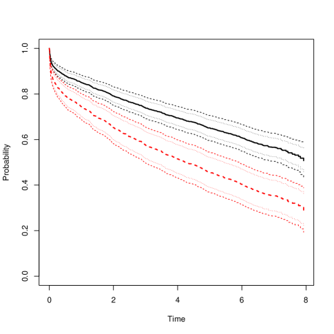
Figure 1: Survival function estimates for males with average age, with (fat broken line) or without diabetes (fat solid line), and 95 % confidence intervals (dotted lines) as well as 95 % bootstrap confidence bands (broken lines).

We note that the hazard ratio related to diabetes is $1.82$ with 95% confidence interval $(1.50,2.18)$. Thus reflecting that diabetes is a factor that leads to increased mortality. More interestingly, seen in connection with absolute level of mortality, this is then reflected in our estimated survival curves for males with average age and with diabetes (lower broken fat curve, with confidence bands and intervals) or without diabetes (upper solid fat curve). We note that the bands are a bit wider than the point-wise intervals. As the latter do not provide simultaneous coverage the bands should be used to provide uncertainty about the entire survival curve as shown in Figure 1.

We finally illustrate how the joint asymptotic distribution of the baseline and the covariates can be used with other functionals. To this end, consider the restricted residual mean

$$\Psi(\Lambda_{0})=\int_{0}^{\tau}\exp(-\Lambda_{0}(s))\mathrm{d}s$$

with estimator $\Psi(\widehat{\Lambda}_{0})$. To get a description of its uncertainty based on the wild bootstrap constructions we can simply apply the functional to the obtained bootstrap samples. It follows that $\sqrt{n}(\Psi(\widehat{\Lambda}_{0})-\Psi(\Lambda_{0}))$ has the same asymptotic distribution as $\sqrt{n}(\Psi(\widehat{\Lambda}_{0}^{*})-\Psi(\widehat{\Lambda}_{0}))$ due to Hadamard differentiability of the functional. Thus, we can easily construct symmetric 95% confidence intervals for the restricted residual mean and their differences based on the bootstrap. The key point being that these are very easy to get at when the bootstrap estimates are at hand.

For example, using the direct wild bootstrap approach based on $dN$ and standard normal multipliers, we find that males with diabetes have a restricted residual mean within the first $5$ years at $3.87(3.74,4.00)$ for males without diabetes and $3.15(2.91,3.41)$ with diabetes. Males with diabetes thus lose $0.71(0.49,0.93)$ years within the first $5$ years. In a similar way confidence intervals for other functionals can be obtained by means of the continuous mapping theorem or the functional delta method.

6 Discussion and further research

Despite their importance, confidence bands are not used much in practice even though there is considerable interest in making survival predictions based on semiparametric regression models such as the Cox model. This is probably due to the fact that the key software solutions do not have confidence bands implemented in this setting. The aim of this work is to investigate some natural and simple wild bootstrap approaches for filling this gap. In particular, we have shown in the Appendix that the proposed bootstrap solutions do asymptotically have the desired properties. A key point in our proofs is the fact that we show the properties of our bootstrap procedures relying solely on martingale arguments. This enormously facilitates the transfer of the classical proofs for the estimators to their wild bootstrap counterparts. It became apparent that this approach generalizes to much more complex models as long as they admit a martingale structure for the involved counting processes. This covers for example Cox models in multi-state models or Fine-Gray regression models for subdistribution functions. A future work will focus on how the procedure can be adapted to more complex designs.

In addition, we consider the finite sample performance of various confidence bands and we see that, when the sample size is too small, one needs to be cautious when constructing such bands. When the sample size is reasonable, however, the bands perform well and should be the preferred way of illustrating the uncertainty of the survival curves.

Another, nice feature of the bootstrap approach is that it provides a very simple tool for constructing confidence intervals for functionals of the parameters of interest. We illustrated this by computing the restricted residual mean based on estimates from the Cox model.

Appendix

Appendix A Proofs

Proof of Lemma 1.

To a large extent, it is possible to parallel the martingale arguments as used in the proofs of Theorems VII.2.1 and VII.2.2 in Andersen et al. (1993). We show the proof for the resampling scheme (12) only; once it has been understood how martingale methods can be applied here, it will be apparent how to conduct the proof for the classical wild bootstrap scheme (9) which entirely consists of martingales.

Proof of 3. We introduce the process $C_{t}^{*}(\bm{\beta})=\sum_{i=1}^{n}(G_{i}+1)[\int_{0}^{t}\bm{\beta}^{\prime}\bm{X}_{i}(s)\mathrm{d}N_{i}(s)-\int_{0}^{t}\log{S_{0}(s,\bm{\beta})}\mathrm{d}N_{i}(s)]$ such that $\nabla C_{\tau}^{*}(\bm{\beta})=\bm{U}_{\tau}^{*}(\bm{\beta})$, where $\nabla$ again denotes the gradient with respect to $\bm{\beta}$. We wish to analyse the asymptotic behaviour of the process

$$X^{*}(t,\bm{\beta})=\frac{1}{n}(C_{t}^{*}(\bm{\beta})-C_{t}^{*}(\widehat{\bm{\beta}}))=\frac{1}{n}\sum_{i=1}^{n}(G_{i}+1)\Big{[}\int_{0}^{t}(\bm{\beta}-\widehat{\bm{\beta}})^{\prime}\bm{X}_{i}(s)\mathrm{d}N_{i}(s)-\int_{0}^{t}\log\frac{S_{0}(s,\bm{\beta})}{S_{0}(s,\widehat{\bm{\beta}})}\mathrm{d}N_{i}(s)\Big{]}$$

whose compensator is $\tilde{X}^{*}(t,\bm{\beta})=\frac{1}{n}\sum_{i=1}^{n}[\int_{0}^{t}(\bm{\beta}-\widehat{\bm{\beta}})^{\prime}\bm{X}_{i}(s)\mathrm{d}N_{i}(s)-\int_{0}^{t}\log\frac{S_{0}(s,\bm{\beta})}{S_{0}(s,\widehat{\bm{\beta}})}\mathrm{d}N_{i}(s)]$.

Indeed, it turns out that functions of the form

$$m:t\mapsto\sum_{i=1}^{n}G_{i}\int_{0}^{t}k_{n,\bm{\beta},i}(s)\mathrm{d}N_{i}(s)$$

are martingales with respect to the filtration given by

$$\mathcal{F}_{t}=\sigma\{N_{i}(s),Y_{i}(s),\bm{X}_{i}(s),G_{i}\cdot N_{i}(v):0\leq s\leq\tau,\ 0\leq v\leq t,\ i=1,\dots,n\},$$

where the function $k_{n,\bm{\beta},i}$ is measurable with respect to $\mathcal{F}_{0}$. To verify this, we consider for $0\leq r\leq t$

$$E[m(t)\mid\mathcal{F}_{r}]=\sum_{i=1}^{n}G_{i}\int_{0}^{r}k_{n,\bm{\beta},i}(s)\mathrm{d}N_{i}(s)+\sum_{i=1}^{n}\int_{r}^{t}k_{n,\bm{\beta},i}(s)\mathrm{d}E(G_{i}N_{i}(s)\mid\mathcal{F}_{r})=m(r)$$

due to $E(G_{i}N_{i}(s)\mid\mathcal{F}_{r})=E(G_{i}N_{i}(s)\mid\mathcal{F}_{0})=E(G_{i}\mid\mathcal{F}_{0})N_{i}(s)=0$ for $r\leq s$. See Dobler (2016) or Bluhmki et al. (2018b) for similar arguments in a nonparametric context. Similarly, it can be shown that $m$ has the predictable variation process given by $\langle m\rangle(t)=\sum_{i=1}^{n}\int_{0}^{t}k_{n,\bm{\beta},i}^{2}(s)\mathrm{d}N_{i}(s),$ and the optional variation process given by $[m](t)=\sum_{i=1}^{n}G_{i}^{2}\int_{0}^{t}k_{n,\bm{\beta},i}^{2}(s)\mathrm{d}N_{i}(s).$

Thus, the predictable variation process of $X^{*}(t,\bm{\beta})$ is given by

$$\langle X^{*}(\cdot,\bm{\beta})-\tilde{X}^{*}(\cdot,\bm{\beta})\rangle(t) =\frac{1}{n^{2}}\sum_{i=1}^{n}\int_{0}^{t}\Big{[}(\bm{\beta}-\widehat{\bm{\beta}})^{\prime}\bm{X}_{i}(s)-\log\frac{S_{0}(s,\bm{\beta})}{S_{0}(s,\widehat{\bm{\beta}})}\Big{]}^{2}\mathrm{d}N_{i}(s)$$

$$=\frac{1}{n^{2}}\sum_{i=1}^{n}\int_{0}^{t}\Big{[}(\bm{\beta}-\bm{\beta}_{0})^{\prime}\bm{X}_{i}(s)-\log\frac{S_{0}(s,\bm{\beta})}{S_{0}(s,\bm{\beta}_{0})}\Big{]}^{2}\mathrm{d}N_{i}(s)+O_{p}(n^{-2}),$$ (16)

where the second equality follows from $\widehat{\bm{\beta}}-\bm{\beta}_{0}=O_{p}(n^{-1/2})$ in combination with the mean-value theorem applied to the function $\bm{\beta}\mapsto S_{0}(s,\bm{\beta})$. Its gradient, where the different partial derivatives are evaluated at different intermediate vectors $\tilde{\bm{\beta}}$ (Feng et al., 2013), is bounded in probability. Hence, we use Conditions 1(a)–(c) in combination with the conditional version of Lenglart’s inequality (Section II.5.2.1 in Andersen et al. 1993) and the fact that $n$ times the compensator of the counting process integral in (16) evaluated at $\tau$ converges in (conditional) probability to a finite function of $\bm{\beta}$ to conclude that $n\langle X^{*}(\cdot,\bm{\beta})-\tilde{X}^{*}(\cdot,\bm{\beta})\rangle(\tau)$ too converges to a finite function in $\bm{\beta}$ in conditional probability as $n\rightarrow\infty$. Furthermore, we use Lenglart’s inequality again to show that the compensator $\tilde{X}^{*}(\cdot,\bm{\beta})$ converges in unconditional probability to

$$f(\bm{\beta})=\int_{0}^{\tau}\Big{[}(\bm{\beta}-\bm{\beta}_{0})^{\prime}s_{1}(s,\bm{\beta}_{0})-\log\frac{s_{0}(s,\bm{\beta})}{s_{0}(s,\bm{\beta}_{0})}s_{0}(s,\bm{\beta}_{0})\Big{]}\lambda_{0}(s)\mathrm{d}s.$$

To see this, we again argue that

$$\tilde{X}^{*}(\cdot,\bm{\beta})=\frac{1}{n}\sum_{i=1}^{n}\Big{[}\int_{0}^{t}(\bm{\beta}-\bm{\beta}_{0})^{\prime}\bm{X}_{i}(s)\mathrm{d}N_{i}(s)-\int_{0}^{t}\log\frac{S_{0}(s,\bm{\beta})}{S_{0}(s,\bm{\beta}_{0})}\mathrm{d}N_{i}(s)\Big{]}+o_{p}(1)$$

for similar reasons as above. Now, this counting process integral has an (unconditional) compensator that converges to $f(\bm{\beta})$ in probability as $n\rightarrow\infty$. Another application of Lenglart’s inequality can be used to show that, $n\rightarrow\infty$, $\tilde{X}^{*}(\cdot,\bm{\beta})\stackrel{{\scriptstyle\mathrm{p}}}{{\rightarrow}}f(\bm{\beta})$ in probability as well. Finally, adding all arguments together, one last application of the conditional version of Lenglart’s inequality implies that $X^{*}(\cdot,\bm{\beta})\stackrel{{\scriptstyle\mathrm{p}}}{{\rightarrow}}f(\bm{\beta})$ in conditional probability as $n\rightarrow\infty$.

Now, we can argue similarly to the proof of Theorem VII.5.2.1 in Andersen et al. (1993): By Condition 1(b)–(d), we have for any $\bm{\beta}$

$$\nabla f(\bm{\beta})=\int_{0}^{\tau}(\bm{e}(s,\bm{\beta}_{0})-\bm{e}(s,\bm{\beta}))s_{0}(s,\bm{\beta}_{0})\lambda_{0}(s)\mathrm{d}s$$

and $\nabla f(\bm{\beta}_{0})=0$. Furthermore,

$$-\nabla^{2}f(\bm{\beta})=\int_{0}^{\tau}\bm{v}(s,\bm{\beta}_{0})s_{0}(s,\bm{\beta}_{0})\lambda_{0}(s)\mathrm{d}s$$

which is positive semidefinite and positive definite for $\bm{\beta}=\bm{\beta}_{0}$; cf. Condition 1(e).

To make the following arguments less ambiguous, we use the subsequence principle for convergence in probability and fix, for any arbitrary subsequence $(n^{\prime})\subset(n)$ another subsequence $(n^{\prime\prime})\subset(n^{\prime})$ such that the conditional convergence in probability $X^{*}(\cdot,\bm{\beta})\stackrel{{\scriptstyle\mathrm{p}}}{{\rightarrow}}f(\bm{\beta})$ given $\mathcal{F}_{0}$ holds almost surely along this subsequence $(n^{\prime\prime})$. This convergence is point-wise in $\bm{\beta}$ and the concave function $f(\bm{\beta})$ has a unique maximum at $\bm{\beta}=\bm{\beta}_{0}$. The random function $X^{*}(\cdot,\bm{\beta})$ is also concave with a maximum at $\bm{\beta}=\widehat{\bm{\beta}}^{*}$ if it exists. We use Theorem II.1 in Appendix II of Andersen and Gill (1982) to conclude the uniformity of the convergence $X^{*}(\cdot,\bm{\beta})\stackrel{{\scriptstyle\mathrm{p}}}{{\rightarrow}}f(\bm{\beta})$. For this reason, the maximizing value $\widehat{\bm{\beta}}^{*}$ of $X^{*}(\cdot,\bm{\beta})$ converges to the maximizing value $\bm{\beta}_{0}$ of $f$ in conditional probability given $\mathcal{F}_{0}$ almost surely along the subsequence $(n^{\prime\prime})$ chosen above. We apply the subsequence principle another time to conclude that the conditional convergence in probability $\widehat{\bm{\beta}}^{*}\stackrel{{\scriptstyle\mathrm{p}}}{{\rightarrow}}\bm{\beta}_{0}$ given $\mathcal{F}_{0}$ holds in probability as $n\rightarrow\infty$. But the same convergence holds for $\widehat{\bm{\beta}}$, so the distance $\|\widehat{\bm{\beta}}^{*}-\widehat{\bm{\beta}}\|$ becomes arbitrarily small in conditional probability.

Proof of 2. Consider $\tilde{D}\bm{U}_{\tau}^{*}(\tilde{\bm{\beta}})=(\nabla(\bm{U}_{\tau}^{*})^{(1)}(\bm{\beta}_{1})^{\prime},\dots,\nabla(\bm{U}_{\tau}^{*})^{(p)}(\bm{\beta}_{p})^{\prime})^{\prime}$ where each $\bm{\beta}_{i}$ is on the line segment between $\widehat{\bm{\beta}}^{*}$ and $\widehat{\bm{\beta}}$. We again use martingale theory to prove the desired conditional convergences. Without loss of generality, let us consider the complete matrix $\tilde{D}\bm{U}_{t}^{*}(\tilde{\bm{\beta}})$ at only one intermediate vector $\tilde{\bm{\beta}}$ on the line segment between $\widehat{\bm{\beta}}^{*}$ and $\widehat{\bm{\beta}}$ because if this matrix converges, then also each row converges, and hence the collection of several such rows converge as desired.

We make use of the following decomposition:

$$-\frac{1}{n}\tilde{D}\bm{U}_{\tau}^{*}(\tilde{\bm{\beta}})=\frac{1}{n}\sum_{i=1}^{n}(G_{i}+1)\int_{0}^{t}\bm{V}(s,\tilde{\bm{\beta}})\mathrm{d}N_{i}(s)=\frac{1}{n}\sum_{i=1}^{n}G_{i}\int_{0}^{t}\bm{V}(s,\tilde{\bm{\beta}})\mathrm{d}N_{i}(s)+\frac{1}{n}\int_{0}^{t}\bm{V}(s,\tilde{\bm{\beta}})\mathrm{d}\sum_{i=1}^{n}N_{i}(s).$$

The first term on the right-hand side is asymptotically equivalent to $\frac{1}{n}\sum_{i=1}^{n}G_{i}\int_{0}^{t}\bm{V}(s,\widehat{\bm{\beta}})\mathrm{d}N_{i}(s)$; indeed, $\|\tilde{\bm{\beta}}-\widehat{\bm{\beta}}\|\stackrel{{\scriptstyle\mathrm{p}}}{{\rightarrow}}0$ given $\mathcal{F}_{0}$ in conditional probability as $n\rightarrow\infty$ and $\bm{V}$ converges uniformly to $\bm{v}$ in both arguments. The remaining term $\frac{1}{n}\sum_{i=1}^{n}|G_{i}|N_{i}(t)$ is $O_{p}(1)$ and, therefore, does not matter.

Hence, we may as well focus on the square-integrable martingale $\frac{1}{n}\sum_{i=1}^{n}G_{i}\int_{0}^{t}\bm{V}(s,\widehat{\bm{\beta}})\mathrm{d}N_{i}(s)$. By using similar martingale arguments as above, i.e. Lenglart’s inequality, it can again be shown that this term is asymptotically negligible.

It remains to analyse $\frac{1}{n}\int_{0}^{t}\bm{V}(s,\tilde{\bm{\beta}})\mathrm{d}\sum_{i=1}^{n}N_{i}(s).$ But, after having again argued why $\tilde{\bm{\beta}}$ can be replaced with $\widehat{\bm{\beta}}$ and given $\mathcal{F}_{0}$, this term is deterministic and its unconditional asymptotic bevahiour is known: it converges in probability to $\int_{0}^{t}\bm{v}(s,\beta_{0})s_{0}(s,\beta_{0})\lambda_{0}(s)\mathrm{d}s$; cf. the proof of Theorem VII.2.2 in Andersen et al. (1993). We conclude that $-\frac{1}{n}\tilde{D}\bm{U}_{\tau}^{*}(\tilde{\bm{\beta}})\stackrel{{\scriptstyle\mathrm{p}}}{{\rightarrow}}\int_{0}^{t}\bm{v}(s,\beta_{0})s_{0}(s,\beta_{0})\lambda_{0}(s)\mathrm{d}s$ in conditional probability given $\mathcal{F}_{0}$ as $n\rightarrow\infty$.

Proof of 1. We make use of the fact that $n^{-1/2}\bm{U}_{t}^{*}(\widehat{\bm{\beta}})=n^{-1/2}\sum_{i=1}^{n}G_{i}\int_{0}^{\tau}[\bm{X}_{i}(s)-\bm{E}(s,\widehat{\bm{\beta}})]\mathrm{d}N_{i}(s)$ defines a square-integrable martingale with respect to the filtration $(\mathcal{F}_{s})_{s}$. This can be shown in the same way as for the other martingales above. Its predictable variation process is given by

$$n^{-1}\langle\bm{U}_{(\cdot)}^{*}(\widehat{\bm{\beta}})\rangle(t)=\frac{1}{n}\sum_{i=1}^{n}\int_{0}^{t}[\bm{X}_{i}(s)-\bm{E}(s,\widehat{\bm{\beta}})]^{\otimes 2}\mathrm{d}N_{i}(s).$$

Similarly as before, this function is (unconditionally) asymptotically equivalent to

$$\frac{1}{n}\sum_{i=1}^{n}\int_{0}^{t}[\bm{X}_{i}(s)-\bm{E}(s,\bm{\beta}_{0})]^{\otimes 2}\mathrm{d}N_{i}(s)$$

$$=\frac{1}{n}\sum_{i=1}^{n}\int_{0}^{t}[\bm{X}_{i}(s)-\bm{E}(s,\bm{\beta}_{0})]^{\otimes 2}\mathrm{d}M_{i}(s)+\frac{1}{n}\sum_{i=1}^{n}\int_{0}^{t}[\bm{X}_{i}(s)-\bm{E}(s,\bm{\beta}_{0})]^{\otimes 2}S_{0}(s,\bm{\beta}_{0})\lambda_{0}(s)\mathrm{d}s.$$

The second term on the right-hand side converges in probability to $\int_{0}^{t}\bm{v}(s,\beta_{0})s_{0}(s,\bm{\beta}_{0})\lambda_{0}(s)$ while the remaining martingale term vanishes asymptotically: its predictable variation process is given by

$$\frac{1}{n^{2}}\sum_{i=1}^{n}\int_{0}^{t}[\bm{X}_{i}(s)-\bm{E}(s,\bm{\beta}_{0})]^{\otimes 4}S_{0}(s,\bm{\beta}_{0})\lambda_{0}(s)\mathrm{d}s,$$

where ${\bf{b}}^{\otimes 4}$ is basically the array of all pairs of entries of the matrices $\bf{b}^{\otimes 2}$ and $\bf{b}^{\otimes 2}$. Clearly, this predictable variation goes to zero in probability since the $\bm{X}_{i}$ are bounded and the functions $\bm{E}$ and $S_{0}$ converge uniformly in probability to bounded functions. It remains to apply Rebolledo’s martingale central limit theorem (Theorem II.5.1 in Andersen et al., 1993) to conclude the asymptotic normality of $n^{-1/2}\bm{U}_{\tau}^{*}(\widehat{\bm{\beta}})$. To this end, we again use the subsequence principle. We see that, given $\mathcal{F}_{0}$ and along subsequences, the conditions of Rebolledo’s theorem are satisfied almost surely; particularly the convergence of the predictable variation process of the square-integrable martingale $t\mapsto n^{-1/2}\bm{U}_{t}^{*}(\widehat{\bm{\beta}})$. Hence, almost surely along any subsequence, this process converges in distribution on the Skorokhod space $D[0,\tau]$ to a zero-mean Gaussian martingale whose covariance function is determined by the limit of the predictable variation process. We have thus shown that $n^{-1/2}\bm{U}_{\tau}^{*}(\widehat{\bm{\beta}})$ converges in distribution to a random vector with a multivariate normal distribution. Another application of the subsequence principle transfers the result to conditional convergence in probability along the original sequence $(n)$. ∎

Proof of Theorem 1.

We only prove the assertion on the “wild bootstrapping the score equations” approach. The applicability of the Lin et al. (1993) multiplier scheme follows along the same lines and is in fact more easily to prove because less applications of the mean-value theorem are required. All in all, we will make use of similar martingale arguments for the wild bootstrapped estimators as in the proof of Lemma 1. To increase readability, some repeating arguments are omitted.

As a first step, paralleling the proof of Theorem VII.2.3 in Andersen et al. (1993), we deduce a useful asymptotic representation of the first part of $\sqrt{n}(\widehat{\Lambda}_{0}^{*}(t,\widehat{\bm{\beta}}^{*})-\widehat{\Lambda}_{0}(t,\widehat{\bm{\beta}}))$, i.e., of

$$\sqrt{n}\sum_{i=1}^{n}(G_{i}+1)\int_{0}^{t}[S_{0}^{-1}(u,\widehat{\bm{\beta}}^{*})-S_{0}^{-1}(u,\widehat{\bm{\beta}})]\mathrm{d}N_{i}(u)$$

$$=-\sqrt{n}(\widehat{\bm{\beta}}^{*}-\widehat{\bm{\beta}})\sum_{i=1}^{n}(G_{i}+1)\int_{0}^{t}\bm{E}(u,\tilde{\bm{\beta}}^{*})S_{0}^{-1}(u,\tilde{\bm{\beta}}^{*})\mathrm{d}N_{i}(u).$$

This equality holds due to a Taylor expansion around $\widehat{\bm{\beta}}$. Here, $\tilde{\bm{\beta}}^{*}$ is on the line segment between $\widehat{\bm{\beta}}^{*}$ and $\widehat{\bm{\beta}}$.

Note that we can replace the intermediate $\tilde{\bm{\beta}}^{*}$ vectors by $\widehat{\bm{\beta}}$ because the resulting error

$$\sum_{i=1}^{n}(G_{i}+1)\int_{0}^{t}[\bm{E}(u,\tilde{\bm{\beta}}^{*})S_{0}^{-1}(u,\tilde{\bm{\beta}}^{*})-\bm{E}(u,\widehat{\bm{\beta}})S_{0}^{-1}(u,\widehat{\bm{\beta}})]\mathrm{d}N_{i}(u)$$ (17)

converges to zero in conditional probability as $n\rightarrow\infty$. Indeed, due to Lemma 1 in combination with Conditions 1(a)–(c), the above difference is bounded by $\frac{1}{n}\sum_{i=1}^{n}|G_{i}+1|o_{p}(1)=o_{p}(1)$. Hence,

$$\sqrt{n}(\widehat{\Lambda}_{0}^{*}(t,\widehat{\bm{\beta}}^{*})-\widehat{\Lambda}_{0}(t,\widehat{\bm{\beta}}))=-\sqrt{n}(\widehat{\bm{\beta}}^{*}-\widehat{\bm{\beta}})\Big{[}\sum_{i=1}^{n}(G_{i}+1)\int_{0}^{t}\bm{E}(u,\widehat{\bm{\beta}})S_{0}^{-1}(u,\widehat{\bm{\beta}})\mathrm{d}N_{i}(u)+o_{p}(1)\Big{]}+W^{*}(t),$$

where $W^{*}(t)=\sqrt{n}\sum_{i=1}^{n}G_{i}\int_{0}^{t}S_{0}^{-1}(u,\widehat{\bm{\beta}})\mathrm{d}N_{i}(u)$. Of the term in square brackets, the following sum vanishes:

$$\sum_{i=1}^{n}G_{i}\int_{0}^{t}\bm{E}(u,\widehat{\bm{\beta}})S_{0}^{-1}(u,\widehat{\bm{\beta}})\mathrm{d}N_{i}(u)=\frac{1}{\sqrt{n}}\Big{(}\frac{1}{\sqrt{n}}\sum_{i=1}^{n}G_{i}\int_{0}^{t}\bm{E}(u,\widehat{\bm{\beta}})\frac{n}{S_{0}(u,\widehat{\bm{\beta}})}\mathrm{d}N_{i}(u)\Big{)}$$

because the term in brackets is a square-integrable martingale with respect to $(\mathcal{F}_{t})_{t}$, and thus asymptotically Gaussian. We conclude that

$$\sqrt{n}(\widehat{\Lambda}_{0}^{*}(t,\widehat{\bm{\beta}}^{*})-\widehat{\Lambda}_{0}(t,\widehat{\bm{\beta}}))=-\sqrt{n}(\widehat{\bm{\beta}}^{*}-\widehat{\bm{\beta}})\Big{[}\int_{0}^{t}\bm{e}(u,\bm{\beta}_{0})\lambda_{0}(u)\mathrm{d}u+o_{p}(1)\Big{]}+W^{*}(t).$$

It remains to analyze $\sqrt{n}(\widehat{\bm{\beta}}^{*}-\widehat{\bm{\beta}})$ and $W^{*}(t)$ jointly. Thereof, $\sqrt{n}(\widehat{\bm{\beta}}^{*}-\widehat{\bm{\beta}})$ is essentially a linear transformation of $\bm{U}^{*}_{\tau}(\widehat{\bm{\beta}})$. Thus, its asymptotic multivariate normality follows from the first two assertions of Lemma 1 in combination with Slutzky’s lemma.

For the joint convergence of $\sqrt{n}(\widehat{\bm{\beta}}^{*}-\widehat{\bm{\beta}})$ and $W^{*}(t)$, we consider the process $t\mapsto(n^{-1/2}\bm{U}_{t}^{*}(\widehat{\bm{\beta}}),W^{*}(t))^{\prime}$ which, for similar reasons as in the proof of Lemma 1 defines a square-integrable martingale with respect to the filtration $(\mathcal{F}_{t})_{t}$. We wish to apply Rebolledo’s martingale central limit theorem (with non-trivial initial sigma field $\mathcal{F}_{0}$) in order to obtain the desired joint conditional central limit theorem which holds in probability. To this end, we analyze the predictable covariation process:

$$\langle n^{-1/2}\bm{U}_{(\cdot)}^{*}(\widehat{\bm{\beta}}), W^{*}\rangle(t)=\sum_{i=1}^{n}\int_{0}^{t}[\bm{X}_{i}(u)-\bm{E}(u,\widehat{\bm{\beta}})]S_{0}^{-1}(u,\widehat{\bm{\beta}})\mathrm{d}N_{i}(u).$$ (18)

Approximating $\bm{E}(u,\widehat{\bm{\beta}})$ on the right-hand side by $\bm{E}(u,\bm{\beta}_{0})$ (then using (4)) and $S_{0}^{-1}(u,\widehat{\bm{\beta}})$ by $S_{0}^{-1}(u,\bm{\beta}_{0})$, a Taylor expansion around $\bm{\beta}_{0}$ and the WLLN show that (18) is asymptotically equivalent to

$$\sum_{i=1}^{n}\int_{0}^{t}[\bm{X}_{i}(u)-\bm{E}(u,\bm{\beta}_{0})]S_{0}^{-1}(u,\bm{\beta}_{0})\mathrm{d}N_{i}(u)$$

$$=\sum_{i=1}^{n}\int_{0}^{t}[\bm{X}_{i}(u)-\bm{E}(u,\bm{\beta}_{0})]S_{0}^{-1}(u,\bm{\beta}_{0})\mathrm{d}M_{i}(u)$$ (19)

$$\quad+\sum_{i=1}^{n}\int_{0}^{t}[\bm{X}_{i}(u)-\bm{E}(u,\bm{\beta}_{0})]S_{0}^{-1}(u,\bm{\beta}_{0})Y_{i}(u)\exp(\bm{X}_{i}^{\prime}(u)\bm{\beta}_{0})\mathrm{d}\Lambda_{0}(u).$$ (20)

By definition of $S_{0}$ and $S_{1}$, the second term (20) on the right-hand side is zero. The remaining term (19) is a martingale with predictable variation

$$\sum_{i=1}^{n}\int_{0}^{t}[\bm{X}_{i}(u)-\bm{E}(u,\bm{\beta}_{0})]^{\otimes 2}S_{0}^{-2}(u,\bm{\beta}_{0})Y_{i}(u)\exp(\bm{X}_{i}^{\prime}(u)\bm{\beta}_{0})\mathrm{d}\Lambda_{0}(u)=\int_{0}^{t}\bm{V}(t,\bm{\beta}_{0})S_{0}^{-1}(u,\bm{\beta}_{0})\mathrm{d}\Lambda_{0}(u)\stackrel{{\scriptstyle\mathrm{p}}}{{\rightarrow}}0.$$

Thus, Lenglart’s inequality implies that the martingale (19) also goes to zero in probability as $n\rightarrow\infty$. Hence, $\sqrt{n}(\widehat{\bm{\beta}}^{*}-\widehat{\bm{\beta}})$ and $W^{*}$ are asymptotically independent.

Likewise, the other predictable variation processes (conditionally) converge as follows:

$$\langle n^{-1/2}\bm{U}_{(\cdot)}^{*}(\widehat{\bm{\beta}})\rangle(t) \stackrel{{\scriptstyle\mathrm{p}}}{{\rightarrow}}\bm{\Sigma}_{t}=\int_{0}^{t}v(u,\bm{\beta}_{0})s_{0}(u,\bm{\beta}_{0})\mathrm{d}\Lambda_{0}(u),$$

$$\langle W^{*}\rangle(t) \stackrel{{\scriptstyle\mathrm{p}}}{{\rightarrow}}\omega^{2}(t):=\int_{0}^{t}\frac{\mathrm{d}\Lambda_{0}(u)}{s_{0}(u,\bm{\beta}_{0})}$$

given $\mathcal{F}_{0}$ in probability by Conditions 1(a) and (b). Finally, applying Rebolledo’s Theorem, it follows that the optional covariation process $I_{t}^{*}(\widehat{\bm{\beta}})$ of $\bm{U}_{t}^{*}(\widehat{\bm{\beta}})$ converges in conditional probability towards $\bm{\Sigma}_{t}$. ∎

References

- Andersen and Gill (1982) PK Andersen and RD Gill. Cox’s regression model for counting processes: a large sample study. The Annals of Statistics, 10(4):1100–1120, 1982.
- Andersen et al. (1993) PK Andersen, Ø Borgan, RD Gill, and N Keiding. Statistical Models Based on Counting Processes. Springer, New York, 1993.
- Beran and Ducharme (1991) RJ Beran and GR Ducharme. Asymptotic theory for bootstrap methods in statistics. Centre de Recherches Mathematiques, 1991.
- Beyersmann et al. (2013) J Beyersmann, S Di Termini, and M Pauly. Weak Convergence of the Wild Bootstrap for the Aalen-Johansen Estimator of the Cumulative Incidence Function of a Competing Risk. Scandinavian Journal of Statistics, 78:387–402, 2013.
- Bluhmki et al. (2018a) T Bluhmki, D Dobler, J Beyersmann, and M Pauly. A wild bootstrap approach for the Aalen-Johansen estimator. Lifetime Data Analysis, early view, doi:10.1007/s10985-018-9423-x, 2018a.
- Bluhmki et al. (2018b) T Bluhmki, C Schmoor, D Dobler, M Pauly, J Finke, M Schumacher, and J Beyersmann. A wild bootstrap approach for the Aalen-Johansen estimator. Biometrics, early view, doi:10.1111/biom.12861, 2018b.
- Cox (1972) DR Cox. Regression models and life-tables (with discussion). Journal of the Royal Statistical Society, Series B, 34(2):187–220, 1972.
- Dobler (2016) D Dobler. Nonparametric inference procedures for multi-state Markovian models with applications to incomplete life science data. PhD thesis, Universität Ulm, 2016.
- Dobler and Pauly (2014) D Dobler and M Pauly. Bootstrapping Aalen-Johansen processes for competing risks: Handicaps, solutions, and limitations. Electronic Journal of Statistics, 8(2):2779–2803, 2014.
- Dobler et al. (2017) D Dobler, J Beyersmann, and M Pauly. Non-strange weird resampling for complex survival data. Biometrika, 104(3):699–711, 2017.
- Dudley (2002) RM Dudley. Real analysis and probability, volume 74 of cambridge studies in advanced mathematics, 2002.
- Efron and Tibshirani (1994) B Efron and RJ Tibshirani. An introduction to the bootstrap. CRC press, 1994.
- Feng et al. (2013) C Feng, H Wang, Han Y, Y Xia, and XM Tu. The Mean Value Theorem and Taylor’s Expansion in Statistics. The American Statistician, 67(4):245–248, 2013.
- Fine and Gray (1999) JP Fine and RJ Gray. A proportional hazards model for the subdistribution of a competing risk. Journal of the American Statistical Association, 94(446):496–509, 1999.
- Jensen et al. (1997) GV Jensen, C Torp-Pedersen, P Hildebrandt, L. Kober, FE Nielsen, T Melchior, T Joen, and PK Andersen. Does in-hospital ventricular fibrillation affect prognosis after myocardial infarction? European Heart Journal, 18:919–924, 1997.
- Lin (1997) DY Lin. Non-parametric inference for cumulative incidence functions in competing risks studies. Statistics and Medicine, 16:901–910, 1997.
- Lin et al. (1993) DY Lin, LJ Wei, and Z Ying. Checking the Cox model with cumulative sums of martingale-based residuals. Biometrika, 80(3):557–572, 1993.
- Lin et al. (1994) DY Lin, TR Fleming, and LJ Wei. Confidence bands for survival curves under the proportional hazards model. Biometrika, 81(1):73–81, 1994.
- Martinussen and Scheike (2006) T Martinussen and TH Scheike. Dynamic regression models for survival data. Statistics for Biology and Health. Springer, New York, 2006.
- Scheike and Zhang (2002) TH Scheike and M-J Zhang. An Additive-Multiplicative Cox-Aalen Regression Model. Scandinavian Journal of Statistics, 29(1):75–88, 2002.
- Spiekerman and Lin (1998) CF Spiekerman and DY Lin. Marginal Regression Models for Multivariate Failure Time Data. Journal of the American Statistical Association, 93(443):1164–1175, 1998.