Relating Kerr SMBHs in Active Galactic Nuclei to RAD configurations

Abstract

There is strong observational evidence that many active galactic nuclei (AGNs) harbour super-massive black holes (SMBHs), demonstrating multi-accretion episodes during their life-time. In such AGNs, corotating and counterrotating tori, or strongly misaligned disks, as related to the central Kerr SMBH spin, can report traces of the AGNs evolution. Here we concentrate on aggregates of accretion disks structures, ringed accretion disks (RADs) orbiting a central Kerr SMBH, assuming that each torus of the RADs is centered in the equatorial plane of the attractor, tori are coplanar and axi-symmetric. Many of the RAD aspects are governed mostly by the spin of the Kerr geometry. We classify Kerr black holes (BHs) due to their dimensionless spin, according to possible combinations of corotating and counterrotating equilibrium or unstable (accreting) tori composing the RADs. The number of accreting tori in RADs cannot exceed $n=2$. We present list of $14$ characteristic values of the Kerr BH dimensionless spin $a$ governing the classification in whole the black hole range $0\leq a\leq M$, uniquely constrained by the RAD properties. The spin values are remarkably close providing an accurate characterization of the Kerr attractors based on the RAD properties. RAD dynamics is richer in the spacetimes of high spin values. One of the critical predictions states that a RAD tori couple formed by an outer accreting corotating and an inner accreting counterrotating torus is expected to be observed only around slowly spinning ($a<0.46M$) BHs. The analysis strongly binds the fluid and BH characteristics providing indications on the situations where to search for RADs observational evidences. Obscuring and screening tori, possibly evident as traces in X-ray spectrum emission, are strongly constrained, eventually ruling out many assumptions used in the current investigations of the screening effects. We expect relevance of our classification of Kerr spacetimes in relation to astrophysical phenomena arising in different stages of AGNs life that could be observed by the planned X-ray satellite observatory ATHENA (Advanced Telescope for High ENergy Astrophysics).

I Introduction

Black hole (BH) physics and the BH accretion disk investigation is developing in the last years. The launch of new satellite observatories in the near future allows an unprecedented close look at situations and contexts which were inconceivable only a few years ago. Observable features on the accreting disks, focusing on morphology of accretion processes and associated jet emissions provide increasingly more detailed and focused pictures of these objects. The sensational opening of a new observational era represented by gravitational waves (GWs) detection allows us to focus on questions of broader interest involving more deeply the BH physics. On the other hand, the theoretical modeling seems to resort deeply to these improvements. Concerning the BH accretion disks processes, there is great expectation towards the X-ray emission sector, with several missions as XMM-Newton (X-ray Multi-Mirror Mission), RXTE (Rossi X-ray Timing Explorer) or ATHENA. Recent studies point out also an interesting possible connection between accretion processes and GWs (Kiuchi et al., 2011). In this scenario, however, many questions remain still unresolved, leaving them as intriguing problems of observational astrophysics, appearing to demand even a greater effort from the point of view of the model development, as the still missing solution of gamma ray bursts (GRBs) origin, the jet launch, the quasi-periodic oscillations (QPOs), the formation of SMBHs in AGNs. In general, the theoretical investigation is increasingly oriented towards the attempt to find a correlation between different phenomena and a broader embedding environment, creating a general framework of analysis envisaging the BH-disk system as a whole. In this sense we may talk about an Environmental Astrophysics. Evidences of this fact are the debates on the jet-accretion correlation, the BH accretion rate-disk luminosity issue, the BH growth–accretion disk and BH–spin shift–accretion disk correlation and BH populations and galaxy age correlation–see for example Lee et al. (2017b); Sadowski et al. (2016); Madau (1988); Ricci et al. (2017b); Narayan & McClintock (2013); Mewes et al. (2016); Morningstar et al. (2014); Yu et al. (2015); Volonteri et al. (2003a); Hirano et al. (2017); Regan et al. (2017); Yang et al. (2017); Xie & Yuan (2017).

In this regard, a crucial aspect to establish correlation between SMBHs and their environment is first the recognition of the BH attractor. Although the unambiguous SMBH identification reduces to assign the BH spin $a$ and mass $M$ parameters or even, for many purposes, only the BH spin-mass ratio $a/M$, this task is still controversial and debated issue of the BH astrophysics. We shall see in fact that many aspects of the BH accretion disk physics depend only on the ratio $a/M$. The issue to identify a rotating BH by determining its intrinsic rotation, or spin-mass ratios, is a rather difficult issue, a complex task which is challenged by different observational and theoretical approaches. All these methods are continuously debated and confronted–see for example Capellupo et al. (2017); McClintock et al. (2006); Daly (2009). It should be noted then that the evaluation of the SMBHs spin is strictly correlated with the “mass-problem”: the assessment of the precise value of the spin parameter of the BH is connected with the evaluation of the main features of the BH accretion disk system, as the BH accretion rate or the location of the inner edge of the accretion disk. The GWs detection from coalescence of BHs in a binary system may serve, in future, as a further possible method to fix a BH spin parameter (Farr et al., 2017; van Putten & Della Valle, 2017; van Putten, 2012, 2015). However, nowadays this task is often approached in BH-accretion disk framework, by considering the evaluation of the mass accretion rate (connected with the disk luminosity) or, for example, the location of the inner edge of an accreting disk. Nevertheless all these aspects are certainly not settled in one univocal picture; for example, even the definition of the inner edge of an accreting disk is very controversial -see for example Krolik & Hawley (2002); Bromley et al. (1998); Abramowicz et al. (2010); Agol & Krolik (2000); Paczyński (2000); Pugliese & Stuchlík (2016, 2018a).

Therefore, GW observations have the ability to provide a “disk”-independent way to trace back the (dimensionless) BH spin and more generally an evaluation of the mass and spin parameters of the black holes – for GW methods for the evaluation of the BH spin see for example Farr et al. (2017); van Putten (2015); van Putten & Della Valle (2017); Pürrer et al. (2016); Andrade-Santos et al. (2016).

In this paper, we face the problem of the black hole identification, proposing an approach which we believe can be promising especially for SMBHs in AGNs. Our investigation is essentially centered on the exploitation of a special connection between SMBHs and their accretion tori; we show that the dimensionless spin of a central BH ($a/M$) and the morphological and equilibrium properties of its accreting disks, are strongly related. Recently, various analyses have shown, in the general relativistic regime, that completely axis-symmetric and coplanar configurations are strongly restricted with regards to their formation, kinematic characteristics (as range of variation of angular momentum) or the emergence of instability. Their existence is constrained according to different evolutionary phases of the individual configurations and, more importantly, by the properties of the central Kerr attractor (Pugliese & Montani, 2015; Pugliese & Stuchlík, 2015, 2016, 2017, 2018a).

More generally, there is a strong relation between the galaxy dynamics and its super-massive guest, specially in the accretion processes. It is expected that such SMBHs in AGNs are characterized by a series of multi-accreting episodes during their life-time as a consequence of interaction with the galactic environment, made up by stars and dust, being influenced by the galaxy dynamics. Further example of the complex and rich black hole-active galaxy interaction is known as feedback AGN– (Ricci et al., 2017a; Almeida & Ricci, 2017; Ricci et al., 2017b; Hirano et al., 2017; Komossa, 2015). These activities may leave traces in the form of matter remnants orbiting the central attractors. Thus, chaotical, discontinuous accretion episodes can produce sequences of orbiting toroidal structures with strongly differing features as, for example, different rotation orientations with respect to the central Kerr BH where corotating and counterrotating accretion stages can be mixed (Dyda et al., 2015; Alig et al., 2013; Carmona-Loaiza et al., 2015; Lovelace & Chou, 1996; Lovelace et al., 2014). Strongly misaligned disks may appear with respect to the central SMBH spin (Nixon et al., 2013; Doğan et al., 2015; Bonnerot et al., 2016; Aly et al., 2015). However, in this work classes of rotating BHs, identified by their dimensionless spin, are associated to particular features of the BH orbiting accreting tori, namely aggregates of toroidal axis-symmetric accretion disks, also known as Ringed Accretion Disks (RADs), centered on the equatorial plane of a Kerr SMBH. The RAD aggregate is composed by both corotating and counterrotating tori, the limiting case of single accretion torus orbiting the SMBH is also addressed as a special case of the RAD. Each RAD toroidal component is modeled by a perfect fluid with barotropic equation of state and constant specific angular momentum distribution (Pugliese et al, 2012; Pugliese & Montani, 2015; Abramowicz & Fragile, 2013; Pugliese & Montani, 2013). RAD models follow the possibility that several accretion tori can be formed around very compact objects as SMBHs ($10^{6}-10^{9}M_{\odot}$, $M_{\odot}$ being solar masses) in AGNs. RAD may be also originated after different accretion phases in some binary systems or BH kick-out, or by local clouds accretion. We mention also Bonnell & Rice (2008) for an analysis of the massive cloud spiraling into the SMBH Galaxy.

More generally, multiple structures orbiting around SMBHs can be created from several different processes involving the interaction between the BH attractors and their environment. An original Keplerian disk can split into two (or more) components (toroids) for some destructive effects where for example the self-gravity of the disk becomes relevant. The impact of the disk self-gravity in different aspects of the BH accretion is discussed in Sec. V. Formation of more tori is also one of the possible endings of a misaligned disk, for example in a binary system, where the torque and warping is relevant to induce a disk fragmentation. In all these cases, the rotational law of newly formed tori can be also very different. In fact, multiple systems can originate in several periods of the accretion life from different material embeddings. In an early phases of their evolution, accretion disks can be misaligned with respect to the equatorial plane of the Kerr attractor and in many cases such disks are expected to be “warped” and “twisted” accretion disks. Although the misaligned or warped case is not covered here, we also discuss the occurrence of this possibility within the RAD frame in Sec. V, where we also address possible instability processes when RAD is extended to consider aggregates with the contribution of the magnetic field. However, misaligned disks, for specific values of the characteristic parameters, will eventually end in a steady state with an inner aligned disk. It has been shown that counterrotating tori can derive also from highly misaligned disks after galaxy mergers, with galactic planes strongly inclined.

Furthermore, in a warped disk scenario the analysis of inner region of accretion disk connected with the jet emission is also considered for the assessment of the central BH spin, assuming that the jet directions are indicative of the direction of the BH spin. We consider this briefly in Sec. V. In the case of misaligned disks, these studies focus on radio–jet direction in AGN along orbital plane direction. More generally, BH and jet emission connection (for example radio and X-ray emission) are considered in galactic embedding to test correlation between the galactic host and jets; the presence of a warped disk can also explain the jet emission orientation with respect to the galactic plane showing also a strong misalignment. Without going into details of this aspect of the accreting process, going beyond the scope of the present work, we mention in particular the case of galaxy NGC4258 (Moran, 2008; Humphreys et al., 2008; Doeleman et al., 2008; Qin et al., 2008; Rodriguez et al., 2008; Kondratko et al., 2008).

Jet emission, in fact, constitutes the third ingredient in the unified BH–accretion disk framework. Almost any BH is associated to a jet emission. How exactly the jet emission and morphology (collimation along the axis, rapidity of emission launch, chemical composition) can be precisely linked or induced by the mechanisms of accretion remains to be clarified. Jets are supposed to be connected with the dynamics of the inner region of the disk in accretion. The role of jet in the BH-accretion disk systems and accretion physics is multiple, altering the energetic of the accretion processes with the extraction of the rotational energy of the central BH and the rotational energy of the disk, and changing the accretion disk inner edge. The inner–edge-jet correlation has to be then framed in the case of the misaligned disks, where the location of the edge is related to the strength of the jet– Neilsen & Lee (2009); Fender & Belloni (2004); Fender (2009); Soleri et al. (2010); Tetarenko et al. (2018); Toba et al. (2017); Fang & Murase (2018); Fender et al. (1998); Fender & Pooley (1998); Fender et al. (1999); Fender (2001). For an analysis of the energetic X-ray transient with associated relativistic jets, updated investigations on jet emission detection see Marscher et al. (2002); Maraschi & Tavecchio (2003); Chen et al. (2015); Yu et al. (2015); Zhang et al. (2015); Sbarrato et al. (2014); Maitra et al. (2009); Ghisellini et al. (2014); Bromley et al. (1998). For jet-accretion disk correlation in AGN see for example Liska et al. (2018); Caproni et al. (2017); Inoue et al. (2017); Gandhi et al. (2017); Duran et al. (2017); Vedantham et al. (2017); Bogdan et al. (2017); Banados et al. (2017); D’Ammando (2017) and also Neilsen & Lee (2009); Fender & Belloni (2004); Fender (2009); Soleri et al. (2010); Tetarenko et al. (2018); Toba et al. (2017); Fang & Murase (2018).

Jet production, as an important additional aspect of the physics of accretion disk, fits into the RAD context in many ways. Firstly, more points of accretion can be present in the RAD inside the ringed structure. It has been shown in Pugliese & Stuchlík (2015) that a RAD, as an aggregated body of orbiting tori, can be considered as a single disk orbiting around a central Kerr attractor on its equatorial plane, with axi-symmetric but knobby surface and diversified specific angular momentum distribution, due to the different contributions of each torus of the RAD agglomerate that can be either corotating or counterrotating with respect to the central attractor. Only for the RAD systems satisfying certain constraints on the BH spin and on the specific angular momentum of the tori, a double accretion phase can occur. Such a situation implies the concomitant presence of two coplanar accreting tori of the RAD in the same period of the BH life. In the frame of accretion disk–jet correlation, this would imply the presence of a shell of double jets, one from an outer counterrotating torus and one associated to the inner corotating accreting torus. Moreover, the geometrically thick tori considered as RAD components are known to be associated to several species of open surfaces (proto-jets) related to emission of matter funnels in jets–Abramowicz & Fragile (2013). These configurations have been discussed in literature in several contexts. The RAD model inherits this characteristic of the accretion torus. The proto-jets, as related to the critical points of the hydrostatic pressure in the force balance of the RAD tori, can give raise to complicated sets of jets funnels either from corotating or counterrotating fluids in more points of the tori agglomeration. We do not consider directly in this investigation the open surfaces, but they will be considered for the classification of the attractors. A more focused analysis on proto-jets in the RAD framework can be found in Pugliese & Stuchlík (2016, 2018a, 2018a).

The plan of this article is as follows. Section  II introduces the model of RAD orbiting a central Kerr attractor: in Sec. II.1 we examine main properties of the Kerr BH exact solution. RAD model is then developed in Sec. II.2 where the toroidal configurations are discussed, and main properties and characteristics of the tori and the macro-structure are presented. The RAD is a relatively new model, this analysis has therefore required the introduction of new concepts adapted to the model. For this purpose it is convenient to introduce a reference Section II.2.1 where we give relevant model details grouping together the main definitions used over the course of this work. We made use also of Table 1 and Table 6 where the symbols and relevant notation used throughout this article are listed. Section III encloses the main results of this work. Tables 2 shows the major classes of attractors considered in this section and, in a compact form, main properties the associated RADs, as investigated in Sec. II.2.1. In Sec. (IV) we concentrate on the double accretion occurring in RAD couples. In Sec. V general discussion on the RAD instabilities and generalizations of the RAD model is presented. We also discuss the possible significance of the tori self-gravity, tori misalignment, viscosity and magnetic field in the RAD. Concluding remarks are in Sec. VI, where we report a brief summary of the results of our analysis, followed by considerations on the impact of the RAD hypothesis in the AGN environments and on some aspects of the phenomenology connected with the RAD. Finally, Appendix follows, where further details on BH spin properties are provided.

II Ringed accretion disks orbiting Kerr attractors

II.1 Geometry and test-particle motion

The Kerr metric line element can be written in the Boyer-Lindquist (BL) coordinates $\{t,r,\theta,\phi\}$ as follows

$$ds^{2}=-dt^{2}+\frac{\Sigma}{\Delta}dr^{2}+\Sigma d\theta^{2}+(r^{2}+a^{2})\sin^{2}\theta d\phi^{2}$$ (1)

$$+\frac{2M}{\Sigma}r(dt-a\sin^{2}\theta d\phi)^{2}\,$$

$$\mbox{where}\quad\Sigma\equiv r^{2}+a^{2}\cos\theta^{2},\Delta\equiv r^{2}-2Mr+a^{2},$$

and $0<a=J/M\leq M$ is the specific angular momentum, $J$ is the total angular momentum of the gravitational source and $M$ is the gravitational mass parameter. The non-rotating limiting case $a=0$ corresponds to the Schwarzschild metric, while the extreme Kerr Black hole has dimensionless spin $a/M=1$. The horizons, $r_{-}<r_{+}$, and the outer static limit $r_{\epsilon}^{+}$, are respectively given by:

$$r_{\pm}\equiv M\pm\sqrt{M^{2}-a^{2}};\quad r_{\epsilon}^{+}\equiv M+\sqrt{M^{2}-a^{2}\cos\theta^{2}};$$ (2)

where $r_{+}<r_{\epsilon}^{+}$ on $\theta\neq 0$ and $r_{\epsilon}^{+}=2M$ in the equatorial plane $(\theta=\pi/2)$. The region $\Sigma_{\epsilon}^{+}\equiv[r_{\epsilon}^{+},r_{+}[$ is known as ergoregion, and the static limit $r_{\epsilon}^{+}$ is also known as outer ergosurface. Because of the symmetries of the Kerr geometry, the quantities

$${E}\equiv-g_{\alpha\beta}\xi_{t}^{\alpha}p^{\beta}=-p_{t},\quad L\equiv g_{\alpha\beta}\xi_{\phi}^{\alpha}p^{\beta}=p_{\phi}\,$$ (3)

are constants of motion, $p^{\alpha}$ is the particle four–momentum and $\xi_{\phi}=\partial_{\phi}$ and $\xi_{t}=\partial_{t}$ are the rotational Killing vector field and the time Killing vector field representing the stationarity of the spacetime Bardeen et al. (1973). The test particle dynamics is invariant under the mutual transformation of the parameters $(a,L)\rightarrow(-a,-L)$. As a consequence of this, we restrict the analysis of the test particle circular motion to the case of positive values of $a$ for corotating $(L>0)$ and counterrotating $(L<0)$ orbits.

II.2 Toroidal configurations

In this work we consider perfect fluid toroidal configurations orbiting a Kerr BH. We take the energy momentum tensor for one-species particle perfect fluid system

$$T_{\alpha\beta}=(\varrho+p)u_{\alpha}u_{\beta}+\ pg_{\alpha\beta},$$ (4)

where $u^{\alpha}$ is a timelike flow vector field and $\varrho$ and $p$ are the total energy density and pressure respectively, as measured by an observer comoving with the fluid with velocity $u^{\alpha}$. We set up the problem symmetries assuming there is $\partial_{t}\mathbf{Q}=0$ and $\partial_{\varphi}\mathbf{Q}=0$, with $\mathbf{Q}$ being a generic spacetime tensor. Accordingly, the continuity equation is identically satisfied and the fluid dynamics is governed by the Euler equation only:

$$(p+\varrho)u^{\alpha}\nabla_{\alpha}u^{\gamma}+\ h^{\beta\gamma}\nabla_{\beta}p=0\,,$$ (5)

where $\nabla_{\alpha}g_{\beta\gamma}=0$, $h_{\alpha\beta}=g_{\alpha\beta}+u_{\alpha}u_{\beta}$ is the projection tensor (Pugliese & Kroon, 2012; Pugliese & Montani, 2015). We then assume a barotropic equation of state $p=p(\varrho)$, the orbital motion with $u^{\theta}=0$ and $u^{r}=0$. Within these conditions, (5) can be written as an equation for the barotropic pressure $p$ as follows:

$$\frac{\partial_{\mu}p}{\varrho+p}=-{\partial_{\mu}W}+\frac{\Omega\partial_{\mu}\ell}{1-\Omega\ell},\quad\ell\equiv\frac{L}{E},$$ (6)

$$W\equiv\ln V_{eff}(\ell),\quad V_{eff}(\ell)=u_{t}=\pm\sqrt{\frac{g_{\phi t}^{2}-g_{tt}g_{\phi\phi}}{g_{\phi\phi}+2\ell g_{\phi t}+\ell^{2}g_{tt}}}.$$

In (6), $\Omega=u^{\phi}/u^{t}$ is the fluid relativistic angular frequency related to distant observers, while $W(r;\ell,a)$ is the Paczyński-Wiita (P-W) potential, expressed in terms of the fluid effective potential $V_{eff}(r;\ell,a)$.

The effective potential $V_{eff}(r;\ell,a)$ reflects the background Kerr geometry through the parameter $a$, and the centrifugal effects through the fluid specific angular momenta $\ell$, here assumed constant and conserved– (Lei et al., 2008; Abramowicz, 2008). The fluid equilibrium is therefore regulated by the balance of the gravitational and pressure terms versus centrifugal factors arising due to the fluid rotation and the curvature effects of the Kerr background, encoded in the effective potential function $V_{eff}$. Analogously to the test particle dynamics, as the fluid effective potential function is invariant under the mutual transformation of the parameters $(a,\ell)\rightarrow(-a,-\ell)$, we can assume $a>0$ and consider $\ell>0$ for corotating and $\ell<0$ for counterrotating fluids, within the notation $(\mp)$ respectively.

We can summarize the properties of the ringed accretion disk (RAD) model introduced in Pugliese & Stuchlík (2015) as a general relativistic model of toroidal configurations, $\mathbf{C}^{n}=\bigcup^{n}\mathrm{C}_{i}$, consisting of a collection of $n$ sub-configurations (configuration order $n$) of complex corotating and counterrotating toroids orbiting in the equatorial plane of a Kerr attractor. RAD features an axially symmetry, “knobby” accretion disk centered on a Kerr BH. RAD tori can be corotating or counterrotating with respect to the central Kerr BH therefore, assuming a $(\mathrm{C}_{a},\mathrm{C}_{b})$ couple with specific angular momentum $(\ell_{a},\ell_{b})$ respectively, we need to introduce the concept of $\ell$corotating toroids, or “ell”corotating, defined by the condition $\ell_{a}\ell_{b}>0$, and $\ell$counterrotating, or “ell”counterrotating toroids defined by the relation $\ell_{a}\ell_{b}<0$. Two $\ell$corotating tori can be corotating, $\ell a>0$, or counterrotating, $\ell a<0$, with respect to the central attractor–see schemes in Figs 1 and tori in Figs 2 and Figs 4.

(1)	(2)	(3)	(4)

Figure 1: Pictorial schemes of a system of coplanar toroids (rings) orbiting a Kerr black hole attractor. Black region is the black hole, gray region is the ergosphere. The distances between the tori and attractor are not in scale. Rings are schematically represented as two-dimensional objects corresponding to the equilibrium topology. The arrows represent the rotation: the dimensionless spin of the attractor $a/M\geq 0$ is considered always positive, $(\mathbf{+;\cdot,\cdot,\cdot})$, “spin-up” in the picture, or vanishing for the limiting case of the static Schwarzschild solution. The fluid specific angular momentum of an accretion disk $\ell$ can be positive, $\ell a>0$, for corotating $(-)$ (“spin-up”) or negative (light gray line), $\ell a<0$, for counterrotating $(+)$ (“spin-down”) (gray line) with respect to the central black hole. The outer third ring is represented by a dashed and double arrowed line, as may be corotating or couterrotating. $\ell$corotating rings $\ell_{i}\ell_{o}>0$ of corotating tori, $(\mathbf{+;+,+,\pm})$, is presented in scheme (1)-this represents the inner configurations of Fig. 4- (b). $\ell$corotating rings $\ell_{i}\ell_{o}>0$ of counterrotating tori, $(\mathbf{+;-,-,\pm})$, is presented in scheme (2) and this represents the inner configurations of Fig. 4-(d). $\ell$counterrotating if $\ell_{i}\ell_{o}<0$ are scheme (3), $(\mathbf{+;+,-,\pm})$, and scheme (4), $(\mathbf{+;-,+,\pm})$-see also Fig. 4-(a) and (c) respectively.

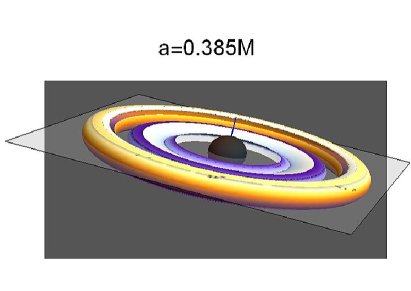
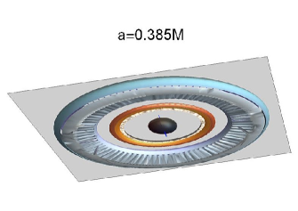
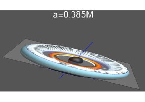
Figure 2: GRHD-Numerical 3D integration of tori density surfaces. Tori are coplanar and orbiting around a central the BH, on the equatorial plane. Colors are chosen according to improved visual effect, integration is stopped at the emerging of disks collision. Black region is $r<r_{+}$, $r_{+}$ is the outer horizon of the black hole of spin $a=0.385M$, gray region is the outer ergosurface. Top panel pictures two coplanar $\ell$counterrotating tori $\mathrm{C}^{+}_{\times}<\mathrm{C}^{-}$, the inner counterrotating torus is accreting onto the central BH, accretion flux is stopped during RAD integration. Center and bottom panels show a RAD sequence $\mathrm{C}^{+}<\mathrm{C}_{o}^{-}\leq\mathrm{C}_{i}^{-}$, made by three $\ell$counterrotating tori: an outer counterrotating torus and an inner couple of colliding corotating toroids. Bottom panel focuses on a different RAD view, featuring the collision of the inner couple, and the separation with respect to the outer counterrotating torus. The entire system BH-RAD is tilted with respect to the observer. The RAD-BH equatorial plane and the spin axis are also shown.

The construction of the ringed configurations is actually in many features quite independent of the model adopted for the single RAD torus (sub-configuration or ring). In fact, in situations where the curvature effects of the Kerr geometry are significant, results are largely independent of the specific characteristics of the model for the single toroidal structure, being primarily based on the characteristics of the geodesic structure the Kerr spacetime related to the matter distribution. To simplify discussion, we consider here each toroid of the ringed disk to be governed by the general relativistic hydrodynamic (GRHD) Boyer condition for equilibrium configurations of rotating perfect fluids. However, these tori are effectively used as initial configurations also for integration in more complex GRMHD models –see for example Lei et al. (2008); Abramowicz & Fragile (2013); Porth et al. (2017). In this approach, the toroidal surfaces are the equipotential surfaces, $V_{eff}=K=$constant, of the effective potential $V_{eff}(\ell,r)$, (Boyer, 1965; Kozlowski et al., 1978) corresponding also to the surfaces of constant density, specific angular momentum $\ell$, and constant relativistic angular frequency $\Omega$, where $\Omega=\Omega(\ell)$ as a consequence of the von Zeipel theorem (Abramowicz, 1971; Zanotti & Pugliese, 2015; Kozlowski et al., 1978). Therefore, each torus is uniquely identified by the couple of $(\ell,K)$ parameters. Assuming a constant specific angular momentum and considering the parameter $K$ related to fluid density, we focus on the solution of the Euler equations associated to the critical points of the effective potential. These solutions, when they exist, represent orbiting configurations which may be closed, quiescent or non accreting $\mathrm{C}$, and cusped $\mathrm{C}_{\times}$ (accreting) toroids, or open, $\mathrm{O}_{\times}$, critical configurations which are associated to some proto-jet matter (Pugliese & Stuchlík, 2016). In general, we use the notation () and $\textbf{()}_{\times}$ to indicate any equilibrium or critical configuration without any further specification of its topology.

The minimum point, $r_{\min}$, of the effective potential (the maximum point for the hydrostatic pressure) corresponds to the center $r_{cent}$ of each toroid. For the cases where a maximum point, $r_{\max}$, exists for the effective potential (the minimum point for the pressure) it corresponds to the critical points, $r_{\times}$, of an accreting torus or, $r_{J}$, for a proto-jet. The open equipotential surfaces have been variously related to “proto jet-shell” structures (Kozlowski et al., 1978; Sadowski et al., 2016; Lasota et. al., 2016; Lyutikov, 2009; Blaschke & Stuchlík, 2016; Madau, 1988; Sikora, 1981; Okuda & Das, 2015). An analysis of these configurations in the RAD framework, has been directly addressed in Pugliese & Stuchlík (2016, 2018a). The inner edge of the Boyer surface is at $r_{in}\in[r_{\max},r_{\min}[$ on the equatorial plane, while the outer edge is at $r_{out}>r_{\min}$ on the equatorial plane as in Figs 4.

The location of the inner and outer edges of the disks is strongly constrained by the geodesic structure of the Kerr spacetime, consisting of the union of the orbital regions with boundaries at the notable radii $R^{\pm}\equiv\{r_{\gamma}^{\pm},r_{\mathrm{mbo}}^{\pm},r_{\mathrm{mso}}^{\pm}\}$.

The set of radii $R^{\pm}$ can be decomposed, for $a\neq 0$, into $R^{-}$ for the corotating and $R^{+}$ for counterrotating matter. Specifically, for timelike particle circular geodetical orbits, $r_{\gamma}^{\pm}$ is the marginal circular orbit or the photon circular orbit, timelike circular orbits can fill the spacetime region $r>r_{\gamma}^{\pm}$. The marginal stable circular orbit $r_{\mathrm{mso}}^{\pm}$: stable orbits are in $r>r_{\mathrm{mso}}^{\pm}$ for counterrotating and corotating particles respectively. The marginal bounded circular orbit is $r_{\mathrm{mbo}}^{\pm}$, where $E_{\pm}(r_{\mathrm{mbo}}^{\pm})=1$ (Pugliese et al., 2011b, 2013, a; Pugliese & Quevedo, 2015; Stuchlík, 1980, 1981a, 1981b; Stuchlík & Kotrlova, 2008; Stuchlík & Slany, 2004) –see Figs 3.

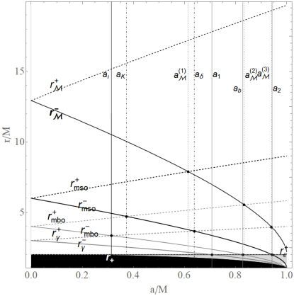
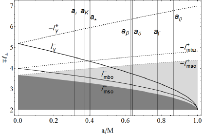
Figure 3: Geodesic structure of the Kerr geometry: notable radii $R\equiv\{r_{\gamma}^{\pm},r_{\mathrm{mbo}}^{\pm},r_{\mathrm{mso}}^{\pm}\}$ (upper panel), and the respective fluid specific angular momenta $\ell^{\pm}_{i}=\ell^{\pm}(r^{\pm}_{i})$ where $r^{\pm}_{i}\in R^{\pm}$, $r_{\mathcal{M}}^{\pm}$ is the maximum point of derivative $\partial_{r}(\mp\ell^{\pm})$ for $a/M$ respectively. Some notable spacetime spin-mass ratios are also plotted, a list can be found in Table 2. Black region is $r<r_{+}$, $r_{+}$ being the outer horizon of the Kerr geometry, gray region is $r<r_{\epsilon}^{+}$, $r_{\epsilon}^{+}$ is the outer ergosurface.

The $\ell$counterrotating sequences are affected strongly by the fact that radii of the sets $R^{+}$ and $R^{-}$, curves $R^{\pm}(a)$, cross in the $(r-a)$ plane–Figs 3 and 5.

There is always $r_{cent}>r_{\mathrm{mso}}^{\pm}$, $r_{\max}\in]r_{\gamma}^{\pm},r_{\mathrm{mso}}^{\pm}]$ and $K_{\pm}\in[K^{\pm}_{\min},K^{\pm}_{\max}[\subset]K_{\mathrm{mso}}^{\pm},1[\equiv\mathbf{K0}$ with specific momentum $\ell_{\pm}\lessgtr\ell_{\mathrm{mso}}^{\pm}\lessgtr 0$ respectively. A one-dimensional ring of matter located at $r_{\min}^{\pm}$ is the limiting case for $K_{\pm}=K_{\min}^{\pm}$.

The specific angular momenta $(\ell_{\gamma}^{\pm},\ell_{\mathrm{mbo}}^{\pm},\ell_{\mathrm{mso}}^{\pm})$, related to $r_{\gamma}^{\pm},r_{\mathrm{mbo}}^{\pm}$, $r_{\mathrm{mso}}^{\pm}$, define three ranges $\mathbf{L1}^{\pm}$, $\mathbf{L2}^{\pm}$, $\mathbf{L3}^{\pm}$ respectively. We denote by the label $i\in\{1,2,3\}$, any quantity $\mathbf{Q}$ related to the range of specific angular momentum $\mathbf{Li}$ respectively; for example, $\mathrm{C}_{1}^{+}$ indicates a closed (regular) counterrotating configuration with specific angular momentum $\ell_{1}^{+}\in\mathbf{L1}^{+}$. No maxima of the effective potential exist for $\pm\ell_{\mp}>\ell_{\gamma}^{\pm}$ ($\mathbf{L3}^{\mp}$) therefore, only equilibrium configurations, $\mathrm{C}_{3}$, are possible. An accretion overflow of matter from the closed, cusped configurations in $\mathrm{C}^{\pm}_{\times}$ (see Fig. 4) towards the attractor can occur from the instability point $r^{\pm}_{\times}\equiv r_{\max}\in]r_{\mathrm{mbo}}^{\pm},r_{\mathrm{mso}}^{\pm}[$, if $K_{\max}\in\mathbf{K0}^{\pm}$ with fluid specific angular momentum $\ell\in]\ell_{\mathrm{mbo}}^{+},\ell_{\mathrm{mso}}^{+}[\equiv\mathbf{L1}^{+}$ or $\ell\in]\ell_{\mathrm{mso}}^{-},\ell_{\mathrm{mbo}}^{-}[\equiv\mathbf{L1}^{-}$. Otherwise, there can be funnels of material along an open configuration $\mathrm{O}^{\pm}_{\times}$, proto-jet or for brevity jet, representing limiting topologies for the closed surfaces (Kozlowski et al., 1978; Sadowski et al., 2016; Lasota et. al., 2016; Lyutikov, 2009; Madau, 1988; Sikora, 1981) with $K^{\pm}_{\max}\geq 1$ ($\mathbf{K1}^{\pm}$), “launched” from the point $r^{\pm}_{\mathrm{J}}\equiv r_{\max}\in]r_{\gamma}^{\pm},r_{{\mathrm{mbo}}}^{\pm}]$ with specific angular momentum $\ell\in]\ell_{\gamma}^{+},\ell_{\mathrm{mbo}}^{+}[\equiv\mathbf{L2}^{+}$ or $]\ell_{\mathrm{mbo}}^{-},\ell_{\gamma}^{-}[\equiv\mathbf{L2}^{-}$–Figs 3 and Figs 5.

However, we can locate the center of each torus more precisely, by introducing the “complementary” geodesic structure $R_{\rho}$, associated to the geodesic structure $R$. (Pugliese & Stuchlík, 2017). This is constituted by the radii $\rho_{j}\in R_{\rho}$, defined as $\rho_{j}>{r}_{j}$ solutions of $\bar{\ell}_{i}\equiv\ell(\rho_{i})=\ell(r_{i})\equiv\ell_{i}$–see Fig. 5 and Figs 3. Radii of $R_{\rho}$ satisfy the same equation as the notable radii $r_{i}\in R$ for corotating and counterrotating configurations, analogously to the couples $r_{\mathcal{M}}^{\pm}$ and $\rho_{\mathcal{M}}^{\pm}$ satisfying relation $r_{\mathcal{M}}^{\pm}>r_{\mathrm{mso}}^{\pm}$, where $\ell_{\mathcal{M}}^{\pm}$ is associated to the maximum of $\partial_{r}|\ell(r)|$– (Pugliese & Stuchlík, 2016). The geodesic structure of the Kerr spacetime and the complementary geodesic structure are both significant in the analysis, especially in the case of $\ell$counterrotating couples. There is $r_{\gamma}^{\pm}<r_{\mathrm{mbo}}^{\pm}<r_{\mathrm{mso}}^{\pm}<\rho_{\mathrm{mbo}}^{\pm}<\rho_{\gamma}^{\pm}$. The location of the radii $r_{\mathcal{M}}$ and $\rho_{\mathcal{M}}$ depends on the fluid rotation with respect to the Kerr attractor. Thus the configurations $\textbf{()}_{1}$ are centered in $]r_{\mathrm{mso}},\rho_{\mathrm{mbo}}[$ (with accretion point in $r_{\times}\in]r_{\mathrm{mbo}},r_{\mathrm{mso}}[$), the $\textbf{()}_{2}$ rings have centers in the range $[\rho_{\mathrm{mbo}},\rho_{\gamma}[$ (with $r_{\mathrm{J}}\in]r_{\gamma},r_{\mathrm{mbo}}[$), finally the $\mathrm{C}_{3}$ toroids are centered at $r\geq\rho_{\gamma}$.

Figures 2 show three dimensional surfaces of special couples of tori obtained by a 3D-GRHD integration.

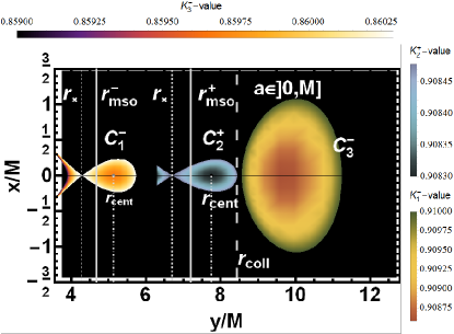
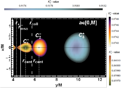
(a)	(b)
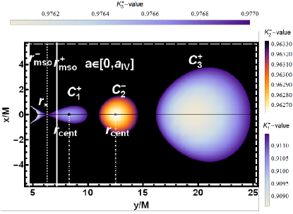
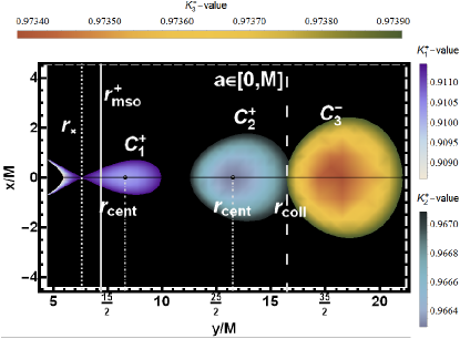
(c)	(d)

Figure 4: GRHD numerical 2D integration of triple toroidal configurations (RADs of the order $n=3$). Tori are coplanar and orbiting on the equatorial plane of a central the BH. (a)-Panel: sequence $\mathrm{C}_{\times}^{-}<\mathrm{C}_{\times}^{+}\leq\mathrm{C}^{-}$. Couple $\mathrm{C}_{\times}^{-}<\mathrm{C}_{\times}^{+}$ may form only around attractors with spin $a>0$, no tori may form between the attractor and the inner accreting corotating torus, while corotating equilibrium tori between the two accreting configurations are possible, see (8). (b)-Panel: sequence $\mathrm{C}_{\times}^{-}\leq\mathrm{C}^{-}<\mathrm{C}^{+}$. (c) -Panel: sequence $\mathrm{C}_{\times}^{+}<\mathrm{C}^{-}<\mathrm{C}^{+}$. Only around the Kerr BHs with spin $a\in[0,a_{IV}[$ the couple $\mathrm{C}_{\times}^{+}<\mathrm{C}^{-}$ can form, no other tori are possible between the central BH and the inner counterrotating accreting ring. (d)-Panel: sequence $\mathrm{C}_{\times}^{+}<\mathrm{C}^{+}\leq\mathrm{C}^{-}$. $(x,y)$ are Cartesian coordinates. Tori notations follow here the relative distance from the attractor in the RAD: thus $\textbf{()}_{1}$ is for the closest and $\textbf{()}_{3}$ for the farthest. Integration is stopped at the emerging of disks collision.

II.2.1 Summary of main notation

This section represents a reference section and provides the summary of the main concepts introduced for the RADs model, see also Table 1. Quantities introduced and discussed here have been grouped according to the properties of the disks or attractors to which they refer.

Table 1: Lookup table with the main symbols and relevant notation used throughout the article.

$\mathrm{C}$	cross sections of the closed Boyer surfaces (equilibrium torus)
$\mathrm{C}_{\times}$	cross sections of the closed cusped Boyer surfaces (accretion torus)
$\mathrm{O}_{\times}$	cross sections of the open cusped Boyer surfaces
()	any of the topologies $(\mathrm{C},\mathrm{C}_{\times},\mathrm{O}_{\times})$
$(r_{in},r_{out})$	inner and outer edge of $\mathrm{C}_{i}$ torus
$\pm$	counterrotating/ corotating
$r_{cent}$	location of torus center
$r_{\times}$	accretion point ( inner edge of accreting torus)
$r_{\mathrm{J}}$	unstable point in open configurations
$r_{coll}$	contact point in collisions among two quiescent tori
$\lessgtr$	tori sequentiality according to the centers $r_{cent}$ (inner/outer disks)
$\prec\succ$	tori sequentiality according to the critical points $(r_{\times},r_{\mathrm{J}})$
$\widehat{\mathbf{C}}_{{m}}$	mixed $\ell$counterrotating sequences
$\widehat{\mathbf{C}}_{{s}}$	isolated $\ell$counterrotating sequences
$\mathfrak{r_{\times}}$	rank maximum number of unstable points $r_{\times}$ in a ringed accretion disk
$\ell_{i/i+1}\equiv\ell_{i}/\ell_{i+1}$	ratio in specific angular momentum of $\mathrm{C}_{i}$ and $\mathrm{C}_{i+1}$
$r^{\pm}_{\mathcal{M}}$	maximum point of derivative $\partial_{r}(\mp\ell^{\pm})$ for given $a/M$

General notations:

Given a radius $r_{\bullet}$

, we adopt the notation $\mathbf{Q}(r):\;\mathbf{Q}_{\bullet}\equiv\mathbf{Q}(r_{\bullet})$ for any function $\mathbf{Q}(r)$.

Notation $r_{\bullet}\in\textbf{()}$

means the inclusion of a radius $r_{\bullet}$ in the configuration () (location of () with respect to $r_{\bullet}$) according to some conditions; $\text{{{$\not$}}}{\in}$ is non inclusion

Notation $\bowtie!$

is an intensifier, a reinforcement of a relation $\bowtie$, indicating that this is a necessary relation which is always satisfied;

Indeces $i$ and $o$

in general define the inner $(i)$ torus, the closest to the central BH and the outer one $(o)$ as there is $\textbf{()}_{i}<\textbf{()}_{o}$, according to notation in Table 1.

Expanded geodesic structure

Alongside the geodesic structure of the Kerr spacetime represented by the set of radii $R\equiv(r_{\mathrm{mso}}^{\pm},r_{\mathrm{mbo}}^{\pm},r_{{\mathrm{\gamma}}}^{\pm},r_{\mathcal{M}}^{\pm})$, we associate the following relations:

$$R_{\rho}\equiv(\rho_{\mathrm{mbo}}^{\pm},\rho_{{\mathrm{\gamma}}}^{\pm},\rho_{\mathcal{M}}^{\pm}):$$ (7)

$$r_{\mathrm{\gamma}}^{\pm}<r_{\mathrm{mbo}}^{\pm}<r_{\mathrm{mso}}^{\pm}<\rho_{\mathrm{mbo}}^{\pm}<\rho_{{\mathrm{\gamma}}}^{\pm}\quad\mbox{where}$$

$$\rho_{\mathrm{mbo}}^{\pm}:\;\ell_{\pm}(r_{\mathrm{mbo}}^{\pm})=\ell_{\pm}(\rho_{\mathrm{mbo}}^{\pm})\equiv\mathbf{\ell_{\mathrm{mbo}}^{\pm}},$$

$$\rho_{{\mathrm{\gamma}}}^{\pm}:\ell_{\pm}(r_{{\mathrm{\gamma}}}^{\pm})=\ell_{\pm}(\rho_{{\mathrm{\gamma}}}^{\pm})\equiv\mathbf{\ell_{{\mathrm{\gamma}}}^{\pm}},$$

$$\rho_{\mathcal{M}}^{\pm}:\ell_{\pm}(\rho_{\mathcal{M}}^{\pm})=\ell_{\mathcal{M}}^{\pm},$$

see Fig. 3 and Fig. 5-top panel. This expanded structure rules good part of the geometrically thick disk physics and multiple structures. The presence of these radii stands as one of the main effects of the presence of a strong curvature of the background geometry.

Notation on the angular momentum $\ell$ and its ranges:

Indices $i\in\{1,2,3\}$ refer to the following ranges of angular momentum $\ell\in\mathbf{Li}$;

Range- L1

$\mp\mathbf{L1}^{\pm}\equiv[\mp\ell_{\mathrm{mso}}^{\pm},\mp\ell_{\mathrm{mbo}}^{\pm}[$ where topologies $(\mathrm{C}_{1},\mathrm{C}_{\times})$ are possible, with accretion point in $r_{\times}\in]r_{\mathrm{mbo}},r_{\mathrm{mso}}]$ and center with maximum pressure $r_{cent}\in]r_{\mathrm{mso}},\rho_{\mathrm{mbo}}]$;

Range- L2

$\mp\mathbf{L2}^{\pm}\equiv[\mp\ell_{\mathrm{mbo}}^{\pm},\mp\ell_{\gamma}^{\pm}[$ where topologies $(\mathrm{C}_{2},\mathrm{O}_{\times})$ are possible, with unstable point $r_{j}\in]r_{\gamma},r_{\mathrm{mbo}}]$ and center with maximum pressure $r_{cent}\in]\rho_{\mathrm{mbo}},\rho_{\gamma}]$;

Range- L3

$\mp\mathbf{L3}^{\pm}\equiv\ \ell\geq\mp\ell_{\gamma}^{\pm}$ where only equilibrium torus $\mathrm{C}_{3}$ is possible with center $r_{cent}>\rho_{\gamma}$;

–see Figs 3.

Mixed and isolated subsequences

We introduce also the following definitions for the $\ell$counterrotating subsequences of a decomposition of the order $n=n_{+}+n_{-}$, of isolated $\ell$counterrotating sequences if $\mathrm{C}_{n_{-}}<\mathrm{C}_{1_{+}}$ or $\mathrm{C}_{n_{+}}<\mathrm{C}_{1_{-}}$, and mixed $\ell$counterrotating sequences, if $\exists\;{i_{+}}\in[1_{+},n_{+}]:\;\mathrm{C}_{1_{-}}<\mathrm{C}_{i_{+}}<\mathrm{C}_{n_{-}}$, or vice versa, $\exists\;{i_{-}}\in[1_{-},n_{-}]:\;\mathrm{C}_{1_{+}}<\mathrm{C}_{i^{-}}<\mathrm{C}_{n_{+}}$, where for example $\mathrm{C}_{i_{-}}$ is the $i$-torus of the corotating subsequence, or alternatively $\widehat{\mathbf{C}}_{{m}}$ ($\widehat{\mathbf{C}}_{{s}}$)-mixed (isolated) $\ell$counterrotating sequences: $[r_{cent}^{1_{-}},r_{cent}^{n_{-}}]\cap[r_{cent}^{1_{+}},r_{cent}^{n_{+}}]\neq(=)0$. Examples of mixed sequences are in Figs 4(a) and (c) panels. Examples of isolated subsequences are in Figs 4-(b) and (d) panel, with an isolated inner corotating subsequence (b) and inner counterrotating isolated sequence (d).

II.2.2 RAD seeds

The study of the aggregate of tori can be carried out considering seed couples. The adoption of this method, used in Pugliese & Stuchlík (2015, 2016), greatly simplifies the characterization of multiple toroidal structures of the order $n>2$. The $n$ order RADs can be investigated starting with analysis of its subsequences of the order $n=2$. Firstly, as the parameters $\{\ell_{i}\}_{i}$ and $\{K_{i}\}_{i}$ are fixed, the RAD is uniquely fixed and therefore it has a unique state, (Pugliese & Stuchlík, 2015). A state consists in the precise arrangement of the following characteristics of the couple: parameters $(\ell_{i},\ell_{o})$ and $(K_{i},K_{o})$, and relative location of the tori edges, topology (if accreting or non accreting torus), if in collision or not .

II.2.3 Some notes on emergence of tori collision and tori correlation

In a seed, tori collision can emerge depending on fixed constraints on the tori. When the seed parameters $(\ell,K)$ are such that these conditions may occur at a certain point of tori evolutions, then we say that the two tori are correlated. As a general result, the correlation is possible in all $\ell$corotating couples $\textbf{()}_{\pm}-\textbf{()}_{\pm}$, according to a proper choice of the density $K$-parameter and specific angular momentum $\ell$. Because of the intrinsic rotation of the Kerr attractor, the correlation in a $\ell$counterrotating couple is disadvantaged and consequently collision may be generally more frequent in a $\ell$corotating couple. This case is in fact mostly constrained by particular restrictions on the specific angular momentum. This situation is obviously less clear in the geometries of the slower BHs. The dynamics of each torus of an $\ell$counterrotating couple is in this sense more “independent” from the other, as tori of these configurations are separated in some extent during their evolutions. A more detailed look at the Table 2, where main spin-classes and their properties are listed, reveals that in the $\ell$counterrotating case the angular momentum is not sufficient to uniquely fix the state and the correlation (indicated with $({\mathrm{\mathbf{C}}})$). Indeed, this depends on the class of the Kerr attractor, and the fluid density through the $K$-parameter. It is found that the proto-jet equilibrium correlation, i.e. a $(\mathrm{O}_{\times}-\mathrm{C})$ couple, is not possible with a corotating proto-jet $\mathrm{O}_{\times}^{-}$, and particularly restrictive conditions are required, if the corotating equilibrium torus is the outer one with respect to the proto-jet configuration. The study of the ranges of the torus edges $(r_{in},r_{out})$ location with respect to the geodesic structure of the Kerr geometry is essential to establish the conditions for tori collision. We therefore studied the inclusions $r_{a}\in\textbf{()}_{i}$ for a configuration $\textbf{()}_{i}$ and a radius $r_{a}\in R^{\pm}$.

Collision may arise, if the edges of tori in a couple are $r_{{in}}^{o}=r_{{out}}^{i}=r_{coll}$, for (non-accreting or accreting) $\ell$corotating or $\ell$counterrotating seed; we indicate this particular colliding seed with notation $\mathbf{\mathrm{C}}_{coll}$. An example of such a case is shown in Fig. 4- (b). This process may eventually lead to tori merging of a kind of drying-feeding process, outlined by a loop evolution in Pugliese & Stuchlík (2016). For example, such a collision can occur as the outer torus grows or loses its angular momentum, approaching the accretion phase. Collisions due to inner torus growing is a particularly constrained case. In general, the emergence of tori collision can be affected by the evolution of the inner torus of a RAD, especially in the early stages of the torus dynamics towards the accretion. The second process related to a tori collision is featured in Fig. 4-(a)-(b) . This process implies emergence of an instability phase for the outer tori of the RAD: the fluid accretion onto the central BH necessarily impacts on the (non-accreting or accreting) inner torus of the couple. Finally, tori collision can emerge also as a combination of the two processes considered before, where there is a contact point, $r_{out}^{i}=r_{\times}^{o}=r_{coll}$ with an accreting outer torus. Collision appears in this case together with an hydro-gravitational destabilization due to the Paczyński-Wiita mechanism (Paczyński, 1980, 2000).

III Relating Kerr Black holes to RAD systems

In this section we consider the properties of RAD aggregate of multiple tori orbiting around a Kerr attractor in relation to its dimensionless spin. Our aim is to provide most complete description of the RAD systems orbiting spinning attractors, characterizing the central Kerr BHs in classes uniquely identifiable through the properties of these objects rotating around them. Findings of our investigation are listed in Table 2 providing an overview of the major features of the classes of spinning attractors, on the basis of the properties of the orbiting toroidal structures. In Table 3 we list some general features of the RAD seeds independent from the BHs spin while in Appendix we discuss more details of the RAD systems and their attractors. Our analysis is conducted by numerical integrating the hydrodynamic equations for multiple systems with fixed boundary conditions for each torus of the set–see Figs 4 and Figs 2. We carefully explored the ranges of fluid specific angular momentum and the tori $K$-parameters, drawing the constraints for the radii $(r_{cent},r_{\times})$ and $(r_{in},r_{out},r_{coll})$ for each torus-see also Pugliese & Stuchlík (2016, 2017, 2018a).

Spin values of Table 2 are remarkably close, consequently ranges of BH attractors are very narrow. This reference table could be therefore used to identify, through some of the RAD features, the properties of the background geometries, placing a Kerr BH, around which a ringed structure can orbit, into one of the particular classes of Table 2. Therefore, we can effectively read Table 2, looking for information on a particular class of attractors, narrowed on a limited dimensionless spin range. Vice versa, for fixed properties of the RADs, we could read the associated class of attractors where these RADs can be found according to Table 2 . This analysis will eventually provide a guide for RAD observations and provide constraints for a dynamical study of RADs evolution in more complex framework, where for example the contribution of magnetic fields is included. Many properties used in the classification actually refer to each single RAD, torus (a limiting RAD of the order $n=1$), independently from the macrostructure. Nevertheless, in the development of the classification in Table 2 we also focused on several BHs-RAD features: the BH dimensionless spin (left column), the tori location (i.e. the specification of $(r_{in},r_{cent})$ and $r_{\times}$ or $r_{\mathrm{J}}$) and relative disposition in the RAD, the emergence of couple instabilities, the fluid specific angular momentum (if $\ell$corotating or $\ell$counterrotating), chance of collision (seed correlation), maximum number of tori in a RAD (the RAD’s order), and general properties of the RAD morphology.

Due to the fact that our analysis includes several properties of each torus of the aggregate and the RAD structure, it is convenient to first introduce some of the main classes, focusing on general tori properties. Thus, below we provide preliminary and general notes on the classification and a description of relevant cases. Specifically we discuss the occurrence of the double accretion phase in the RAD and the presence of possible screening RAD tori. Concluding this part, we examine more closely the tori couples of the seed–schemes of Figs 1, particularly the case with an inner counterrotating torus. We then concentrate our discussion on specific notable BH spins, by describing the main RADs and attractors properties in a defined range of spins.

III.1 Double accretion phase in the RAD and appearance of screening tori.

As a general result, the maximum number of critical points in a RAD can be two. This very special RAD, featuring a double accretion, can be observed only in the spacetimes where $a>0$, therefore it is a characteristic of all the Kerr spacetimes. These aggregates are particularly favored by fast spinning BHs. In such configurations the inner torus in accretion should always be corotating and it has to be the inner torus of the accreting couple as also shown in Figs 4. Then, the outer torus, which is not necessarily adjacent to the inner accreting one, must necessarily be the inner of the counterrotating subsequence of the RAD. The only possible scheme for multi-tori with double accretion is the following:

$$\mbox{for}\quad 0<a\leq M:$$

$$\underset{\textbf{(a)}}{\underbrace{\mathbf{\mathrm{C}_{\times}^{-}}}}<\underset{\textbf{(b)}}{\underbrace{...<\mathrm{C}^{-}<...}}<\underset{\textbf{(c)}}{\underbrace{\mathbf{\mathrm{C}_{\times}^{+}}}}<...\underset{\textbf{(d)}}{\underbrace{<\mathrm{C}^{\pm}<}}...$$ (8)

where $\mathbf{(a)}$ is the inner corotating torus in accretion, $\mathbf{(b)}$ is the inner subsequence of corotating tori in equilibrium, $\mathbf{(c)}$ is the outer counterrotating accreting torus and $\mathbf{(d)}$ is the outer (mixed or separated) subsequence composed of corotating or counterrotating quiescent tori. In Fig. 4- (a)-panel is an example of a RAD of the order $n=3$, $\mathrm{C}_{\times}^{-}<\mathrm{C}_{\times}^{+}<\mathrm{C}^{-}$, with vanishing $\mathbf{(b)}$ component of the corotating inner sequence of Eq. (8). The BHs spin constrains the specific angular momentum, elongation, and number $n$ of tori in the subsequences $\mathbf{(b)}$ and $\mathbf{(d)}$.

In the special RAD of Eq. (8), the subsequence $\mathbf{(b)}$ is made up by “screening” corotating, quiescent tori, between the two accreting tori of the agglomerate. We should also note that no torus, quiescent or in accretion, can form between the central BH and the inner accreting $\mathrm{C}_{\times}^{-}$ configuration.

III.2 Preliminary notes on the counterrotating inner tori.

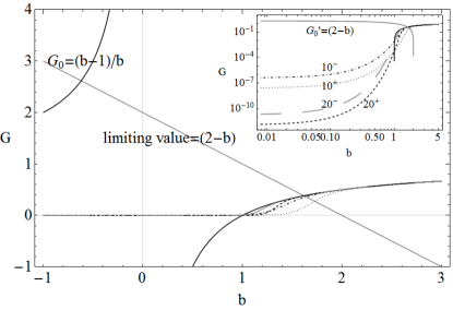
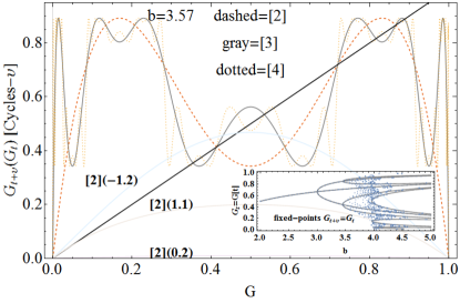
Figure 12: Upper Panel: $\mathrm{G}^{\pm}$ as functions of the parameter $b$. Plots shows fixed point $\mathrm{G}_{0}=(b-1)/b$ and $(2-b)$-limiting function for the stability analysis. Initial data for the accretion rates are $\dot{M}^{+}[0]=0.00054$ for the outer counterrotating torus and $\dot{M}^{-}[0]=0.00845$ for the inner corotating torus related to functions $\Pi$ in Figs 9, taken for a=$0.9M$. Inside panel is a zoom for restricted range of $b$, numbers close to curves are different times $t/M$, signs $\mp$ correspond to the corotating/counterrotating fluids. Bottom panel: Stability analysis, emergent chaos, cycles $\mathrm{G}_{t+\upsilon}(\mathrm{G}_{t})$. Different cycles $\upsilon$ are given in square brackets, numbers close to the curves are for $b$-parameter for the corotating torus. Inner panel: analysis of the fixed points $\mathrm{G}(t+\upsilon)=\mathrm{G}(t)$ versus parameter $b$ for different cycles $(\upsilon)$; some bifurcations appear, for example at $b\approx 3$, $b\approx 3.5$–see also Figs 11.

We consider the schemes in Figs 1 and the geodesic structure in Figs 3 and 13. The innermost stable orbit in counter–rotation, $r_{mso}^{+}$, increases with the dimensionless BH spin, or $\partial_{a}r_{mso}^{+}>0$ (dimensionless units). Whereas the corresponding corotation radius decreases with $a$, or $\partial_{a}r_{mso}^{-}<0$, due to the corotation and the geometry frame dragging, which acts oppositely on the $\ell$counterrotating tori. This implies that with increasing BH dimensionless spin, $a/M$, the difference $r_{\mathrm{mso}}^{+}-r_{\mathrm{mso}}^{-}$ increases. The maximal difference occurs for attractors with the extreme maximal spin value $a=M$. This fact has interesting implications on the RAD stability and the possibility to observe RAD couples. Increasing $\Delta r_{\mathrm{mso}}\equiv r_{\mathrm{mso}}^{+}-r_{\mathrm{mso}}^{-}$ with the spin implies $\partial_{a}\Delta r_{\mathrm{mso}}>0$. This fact has consequences on the formation of the $\ell$counterrotating couples and on their dynamics. The radius $r_{mso}$ is an equilibrium discriminant for the tori, fixing the regions of the maximum and minimum of the hydrostatic pressure in the tori. Similar relations, $\partial_{a}\mathcal{Q}^{\pm}\gtrless 0$ and $\partial_{a}\Delta\mathcal{Q}>0$, hold for $\Delta\mathcal{Q}$ defined analogously to $\Delta r_{\mathrm{mso}}$, where $\mathcal{Q}\in{R,R_{\rho}}$. As discussed in Sec. II.2 and Sec. II.2.1, these radii regulate the equilibrium and the extension of the torus on the equatorial plane as well as other morphological characteristics of the tori as the geometrical thickness. Considering these relations and Figs 3-13, a double accretion for the couple $\mathrm{C}^{-}<\mathrm{C}^{+}$, scheme (4) of Figs 1, is therefore favored by high BH spins–Figs 4. This also has consequences on the energetics of the processes associated to the RAD, the mass accretion rates, the torus cusp luminosity, as well as other tori characteristics depending on the location of the tori inner edge and BH parameters–Pugliese & Stuchlík (2018a). On the other hand, schemes(1) and (3) of Figs 1 feature an inner corotating torus where the outer toroidal disk is corotating and quiescent, scheme (1), and counterrotating in scheme (3). The Lense–Thirring (L-T) effect plays an essential role for these couples. The inner torus, orbiting fast spinning BH attractors, is strongly dominated by the L-T effect and can also form in the ergoregion being generally also rather small. Such accreting tori can also influence heavily the BH attractor, establishing a runaway instability, or extracting energy through jet emission. The increase of the BH spin $a$, favors tori collision in the RAD $\ell$corotating couples formed by corotating tori (see the narrowing of the regions bounded by the radii in $R^{-}$ and $R_{\rho}^{-}$ as shown in Figs 3 and 13). Schemes (2) and (4) of Figs 1 feature an inner counterrotating torus, which is part of the $\ell$corotating couple, $\mathrm{C}^{+}<\mathrm{C}^{+}$, in scheme (2), and component of the $\ell$counterrotating couple, $\mathrm{C}^{+}<\mathrm{C}^{-}$, as represented in scheme (4)–see also Figs 4. Increasing the spin $a$, the inner $\mathrm{C}^{+}$ torus can be observed also far away from the central BH, but accretion is still possible because of the conditions on the radii $R$ and $R_{\rho}$. Considering scheme (4), couples $\mathrm{C}^{+}<\mathrm{C}^{-}$, inner counterrotating torus and outer corotating torus are expected to be observed especially in the geometries of the slow rotating attractors–Figs 4. We shall detail this case below, within the attractors classification. Here we note that the outer, corotating, quiescent torus of this couple, can approach the instability only in the spacetimes of the slower spinning attractors (accretion is always associated to a decrease of the magnitude of the fluid specific angular momentum in the range L1, and to an increase of $K$-parameter where the torus inner edge moves inwardly towards the central attractor). The presence of an outer corotating torus, $\mathrm{C}^{-}$, of the RAD couple in scheme (4) implies, during the RAD evolution, and especially with the emergence of the outer torus instability, the tori collision. This process can also end in a disrupting phenomena, leading eventually to the tori merging. Therefore, this couple could be generally considered as a feature proper of the slower spinning BH. At fixed spin, shifting the torus center outwardly, the accreting torus will be larger than the accreting tori close to the central BH. On the other hand, the increase of the BH spin has similar effects, facilitating larger counterrotating tori and smaller corotating tori very close to the BH, located eventually in the ergoregion Pugliese & Montani (2015). These effects are investigated in Pugliese & Stuchlík (2015, 2017) and in Pugliese & Stuchlík (2018a).

We proceed now by considering some specific notable spins of Table 5 in connection with the principal RAD characteristics. Firstly we discuss the case of a static Schwarzschild BH and then we concentrate on the Kerr BHs, by evaluating the influence of the spin of the central attractor examining first the slower spinning SMBHs singled out from Table 5.

III.3 Schwarzschild attractors $(a=0)$

In the static geometry described by the Schwarzschild metric any RAD sequence of tori behaves as an $\ell$corotating sequence, independently of the relative rotation of fluid in the ringed disk, because of the unique geodesic structure of the spacetime. As consequence of this, accretion around these attractors may occur only from the inner torus of the RAD, while any further torus must be non-accreting (quiescent). Moreover, there can be no screening inner torus, comprised between the outer accreting torus and the central attractor. This implies also that any further torus of the aggregate, shall be outer with the respect to the accreting inner one. The tori sequences are characterized by the outer in the RAD with respect to the inner torus in accretion. For $a=0$ a RAD seed can be only in the following configurations $\textbf{()}_{\pm}<\mathrm{C}_{\pm}$ or $\textbf{()}_{\pm}<\mathrm{C}_{\mp}$. Then an emission spectrum from this RAD should give track as the single accretion inner edge only–in agreement with Schee & Stuchlík (2009, 2013); Sochora et al. (2011); Karas & Sochora (2010). Collision in this geometry is possible according to specific conditions on the fluid density and angular momentum and, in case of emergent Paczyński instability for one of the outer tori of the sequence, collision is inevitable. One torus may evolve from a non-accreting phase to accretion due to decrease of the angular momentum followed by an increase of the torus elongation on the equatorial plane, approaching the attractor. This phenomenon can be detected as a very violent event with large energy release as shown in the first evaluation of energy collision in Pugliese & Stuchlík (2018a). RAD aggregates, orbiting a static attractor, shall therefore characterize the earlier phases of evolution of a RAD, where all the tori, but the inner one, are in equilibrium. It is clear than that these considerations for the static BHs, hold in some extent also for very slowly spinning Kerr BHs: in fact the study of the Schwarzschild case can be seen as the limiting for a Kerr BH where we can consider a “non-relevant” influence of the frame-dragging. The classification specifies the limits on the attractor spin and the RAD features which are mainly affected. As mentioned above a mixed sequences or $\ell$counterrrotating couples are to be considered as $\ell$corotating in the Schwarzschild spacetime because of the equivalences $R^{+}=R^{-}$ and $R_{\rho}^{+}=R_{\rho}^{-}$, as clear also from Figs 3, and 5.

In general, in the case of a spinning Kerr BH, the physics associated with the RADs is much more complex and phenomenology is much more rich as will be discussed in the following section. Following Table 2, we explore the RAD in the Kerr spacetimes by starting with the small spins. Classes in the Table are indicated by arrows, the center column to be read for decreasing spin, down-to-up direction, the right column to be read for increasing spin, up-to-down direction. Thus, for example, considering spin $a_{u}$, Table 2 provides information on the ranges $a<a_{u}$ and $a>a_{u}$ respectively.

III.4 Kerr Black holes $(a\neq 0)$

In the case of axi-symmetric attractors the situation is complicated due to the non-zero intrinsic spin $a$ of the attractor and the relative rotation of the RAD tori. The situation has been addressed in details for ringed disks of the order $n=2$ in Pugliese & Stuchlík (2017). Below we describe the situation considering some remarkable values of dimensionless spin with reference to Table 5. These notable dimensionless spin ranges identify different classes of Kerr attractors, according to their dimensionless spin $a/M$. The representation of the main classes defined is pictured schematically on Fig. 13-Appendix B– note that there are many intersected BH-classes. Some general results, holding irrespectively of the attractor spin-values $a\neq 0$, are listed in Table 5. In the following we focus our discussion on the special spin ranges defined by Kerr BHs spins (I) $a_{\delta}=0.638285M$; (II) $a_{\iota}=0.3137M$; (III) $a_{\mathcal{M}}^{(3)}=0.934313M$; (IV) $a_{IV}=0.461854M$; (V) $a_{u}=0.47403M$; (VI) $a_{VI}=0.73688M$; (VII) $a_{K}=0.372583M$.

To simplify our discussion on the seed couples, in the following we make use of the notation $(\textbf{()},\lessgtr,\prec\succ)$ of Table 1, for the relative location of the tori in the couples and their state of quiescence or instability, as well as the range of variation of the magnitude of the specific angular momentum–see also Sec. II.2.1.

I: [Kerr BHs spin $a_{\delta}$ ]

The first class of attractors we consider are the fastest Kerr BHs having spin $a_{\delta}<a\leq M$. Attractors with values of $a/M$ in this range, have been singled out because couples $\mathrm{C}_{\times}^{-}\prec\mathrm{O}_{\times}^{+}$, formed by a corotating accreting torus with an outer counterrotating proto-jet, can be observed only in these geometries.

II: [Kerr BHs spin $a_{\iota}$ ]

On the other hand, only in the spacetimes where $a_{\iota}<a\leq M$ it is possible to find the couple of proto-jets $\mathrm{O}_{\times}^{-}\prec\mathrm{O}_{\times}$, where the inner configuration is corotating while the outer can be corotating or counterrotating. More specifically, jet-jet correlation, with the production of this double-shell configuration of proto-jets, is always possible except for the fast attractors, class $\mathbf{A_{\iota}^{>}}$, where the case of an outer counterrotating proto-jet is prohibited. Vice versa for slower spinning Kerr BHs, class $\mathbf{A_{\iota}^{<}}$, any combinations of proto-jets are possible.

III: [Kerr BHs spin $a_{\mathcal{M}}^{(3)}$]

Spin $a_{\mathcal{M}}^{(3)}$, introduced in Table 2, discriminates the behavior of corotating and counterrotating tori located far from the source-see Figs 3. Radii $r_{\mathcal{M}}^{\pm}$ and corresponding specific angular momenta $\ell_{\mathcal{M}}^{\pm}$ play an important role in the characterization of the classes of attractors defined by this special spin. In fact, radii $(r_{\mathcal{M}},\rho_{\mathcal{M}})$ and the angular momenta $\ell_{\mathcal{M}}$ regulate the tori angular momentum also in region far from the source, i.e., $r>r_{\gamma}^{\pm}$. Radii $r_{\mathcal{M}}$ and $\rho_{\mathcal{M}}$ play a role in tori formation and, particularly, their collision (Pugliese & Stuchlík, 2016). Indeed, radii $r_{\mathcal{M}}^{\pm}(a)>r_{\mathrm{mso}}^{\pm}$ correspond to the maximum point of the variation of the magnitude of the tori fluid specific angular momenta $\ell$ with respect to the orbital distance from the attractor; they are the solutions of $\partial_{r}\partial_{r}\ell=0$, providing the maximum point of the functions $\mp\partial_{r}\ell^{\pm}$, respectively–Table 1. This means that increasing of the magnitude of the specific angular momentum with the radial distance from the attractor is not permanent, but there is a limiting radius, which is different for the $\ell$counterrotating subsequences-see Fig. 5-bottom panel. We specify the situation below. The maximum $\ell_{\mathcal{M}}$ is associated to a torus centered at $r_{\mathcal{M}}$, having critical point at $\rho_{\mathcal{M}}$ (see definition 7). This implies that the tori of $\ell$corotating couple with fixed angular momentum magnitude difference, $\ell_{o}-\ell_{i}=\epsilon$, are increasingly closer to the central BH as their angular momentum approaches the limiting value $\ell_{\mathcal{M}}$. Noticeably this is a relativistic effect that disappears in the Newtonian limit when the orbital distance is large enough with respect to the radius $r^{\pm}_{\mathcal{M}}$. On the other hand, in the case of static spacetimes, the Schwarzschild BH has $r^{+}_{\mathcal{M}}=r^{-}_{\mathcal{M}}$. Therefore, the existence of the $(r_{\mathcal{M}},\ell_{\mathcal{M}})$ is a relativistic effect, present also in the static case $a=0$, but for a rotating attractor this is strongly differentiated from an albeit minimal intrinsic rotation of the gravitational source. Furthermore, this behavior of the specific angular momentum strongly distinguishes the two $\ell$corotating subsequences of corotating and counterrotating tori. As there is $\partial_{|a|}r_{\mathcal{M}}^{\mp}\lessgtr 0$, for corotating and counterotating tori respectively, the region where less additional specific angular momentum is due increases with the spin-mass ratio of the central BH in the corotating case, while it decreases with the spin in the other case–there is $\partial_{r_{cent}}|\ell_{r_{cent}}|>0$ $\forall r_{cent}$, but $\partial^{2}_{r_{cent}}|\ell_{cent}|>0$ up to a $r_{\mathcal{M}}$, which corresponds to the ring with the center located on $r_{\mathcal{M}}$ where $\partial^{2}_{r_{cent}}|\ell_{cent}|=0$. Then there is $\partial^{2}_{r_{cent}}|\ell_{cent}|<0$ for $r_{cent}>r_{\mathcal{M}}$, or also: $\partial_{r_{cent}}\left.\delta\ell_{cent+j,cent}\right|_{\mathrm{J}}\gtreqqless 0$ for $r_{cent}\lesseqqgtr r_{\mathcal{M}}$, and $r_{cent}\in]r_{\mathrm{mso}},+\infty[$. These results apply in any Kerr spacetime, but depending on the attractor spin, the maximum $r_{\mathcal{M}}$, being a function of $a$, is located in different orbital regions–see Fig. 3. For the case of corotating tori, the region of increasing gap of specific angular momentum decreases with the spin; that is, increasing of the BH spin corresponds to a decrease of the additional specific angular momentum to be supplied to locate the ring centers in an exterior region. In general, one could say that if the $\ell$corotating tori are corotating with respect to the BH we need less additional specific angular momentum to locate outwardly ($\ell$corotating and corotating) tori with respect to the counterrotating case. In this sense, one could also say that the corotation with respect to the BH has a stabilizing effect for the RAD structure. Conversely, in terms of the criticality indices $r_{j}$ (location of critical points), there is $\partial_{r_{\mathrm{J}}}\ell<0$, with $\partial^{2}_{r_{\mathrm{J}}}\ell=0$ for a configuration with specific angular momentum magnitude $\ell_{\mathcal{M}}>\ell_{\mathrm{mbo}}$, centered in $r_{\mathcal{M}}$.

Indeed, since $r_{\mathcal{M}}^{\pm}>r_{\mathrm{mso}}^{\pm}$, the radii $r_{\mathcal{M}}^{\pm}$ can be minimum points of the effective potential, but not maximum points. Then $\ell_{\mathcal{M}}$ is a maximum value for the function $\partial_{r_{cent}}\ell_{r_{cent}}=\partial_{r_{cent}}r_{j}\partial_{r_{j}}\ell_{r_{j}}$. The $\ell$corotating sequences of corotating and counterrotating open configurations with specific angular momentum $\ell_{\mathcal{M}}^{\pm}$ have generally different topologies associated with their critical phase. In fact, for the counterrotating tori around attractors with $0<a\leq M$, we have $-\ell_{\mathcal{M}}\in\mathbf{L2}^{+}$; therefore, critical configurations with $\ell=\ell_{\mathcal{M}}^{+}$ always correspond to the proto-jets $\mathrm{O}_{\times}^{+}$. Conversely, this is not always the case for the corotating tori where, at higher spin of the attractor, i.e., $a\geq a_{\mathcal{M}}^{(3)}$, there is $\ell_{\mathcal{M}}^{-}\in\mathbf{L3}^{-}$, where there are no critical topologies, while in the geometries with $0\leq a<a_{\mathcal{M}}^{(3)}$ there is $\ell_{\mathcal{M}}^{-}\in\mathbf{L2}^{-}$, and only critical configurations $\mathrm{O}_{\times}^{-}$ are possible. Summarizing, the tori centers are more spaced in the region $r>{r}_{\mathcal{M}}$, and vice versa at $r<{r}_{\mathcal{M}}$; the tori are closer each other as they approach ${r}_{\mathcal{M}}$. In conclusion, in a ringed model, where the specific angular momentum varies (almost) monotonically with a constant step $\kappa$, two remarkable points in the distribution of matter appear: the radius $r_{\mathcal{M}}$, where the density of stable configurations reaches the maximum (the maximum hydrostatic pressure), and the corresponding point $\rho_{\mathcal{M}}$ where the density of jet launch is at minimum.

IV: [Kerr BHs spin $a_{IV}$]

Spin $a_{IV}$ identifies one of the most remarkable classes of Kerr BHs in our classification. We detail the properties of the RAD orbiting attractors of these classes as follows. For the faster spinning BHs with $a>a_{IV}$, there are no $\textbf{()}^{+}<\textbf{()}_{1}^{-}$ couples (that is with an inner counterrotating configuration and outer corotating one with $\ell\in\textbf{L1}$), whereas it is possible to find a $\textbf{()}_{1}^{+}<\textbf{()}_{i}^{-}$ couple with $i\in\{2,3\}$, in the BH geometries where $a_{IV}<a<a_{VI}$. This is a strong constraint on the specific angular momenta and on the evolution of the couple tori, which we can read as follows: if the counterrotating inner torus has specific momentum $\ell^{+}\in\textbf{L1}^{+}$, thus in a possible phase of accretion, the corotating outer torus must have a sufficiently large momentum, $\ell_{i}^{-}\neq\ell_{1}^{-}$, which also implies that torus must be sufficiently far from the central attractor and that this couple can only be observed by having a quiescent outer torus (or proto-jet); we refer to Figs 5.

Finally only in the geometry of slower spinning BHs, where the spin is $a<a_{IV}$ (including also the Schwarzschild BH with $a=0$), the couple made up by an inner counterrotating configuration and outer corotating, quiescent or accreting one, with angular momentum $\ell^{-}\in\textbf{L1}^{-}$, that is the seed $\textbf{()}^{+}<\textbf{()}_{1}^{-}$, can be found with initial state having tori $\textbf{()}_{1}^{+}<\textbf{()}_{1}^{-}$, which means an inner counterrotating, quiescent or accreting, torus with $\ell^{+}\in\textbf{L1}^{+}$. This fact makes this class a very special case. In fact, Kerr BHs belonging to this class of attractors constitute the only spacetimes where couples of the kind $\textbf{()}_{1}^{+}<\textbf{()}_{i}^{-}$ for $i\in\{1,2,3\}$, can be observed (inner counterrotating, quiescent or accreting torus with $\ell^{+}\in\textbf{L1}^{+}$, with an outer corotating configuration) and, in particular, RAD tori $\textbf{()}_{1}^{+}<\textbf{()}_{1}^{-}$ (inner counterrotating, quiescent or accreting torus, with an outer corotating torus with angular momenta $\ell^{\pm}\in\textbf{L1}^{\pm}$ respectively) can orbit only around these attractors. As discussed above, these are the only couples where a double accretion phase in the RAD is possible. On the other hand,

$$\mbox{for }\quad 0<a<a_{IV},\quad\mbox{tori as }\quad\mathrm{C}_{\times}^{+}<\mathrm{C}^{-},$$ (9)

can be observed, i.e., an inner counterrotating accreting torus and an outer corotating (non-accreting) torus–see Fig. 4. A couple of tori $\textbf{()}^{+}<\mathrm{C}^{-}$ can be observed around any Kerr BH attractor with $0\leq a\leq M$ (note that we did not specify the range of the specific angular momentum), but only if the central BH has spin in the range $0\leq a<a_{IV}$, the corotating outer torus of the couple $\mathrm{C}^{-}$ approaches the instability phase, i.e. there is $r_{\times}\gtrapprox r_{\mathrm{mso}}^{-}$. The faster spinning is the Kerr BH, the farther away ($r_{cent}>\rho_{\gamma}^{-})$ should be the outer torus to prevent tori collision .

V: [Kerr BH spin $a_{u}$]

Spin $a_{u}$ defines two classes of BHs particularly significant from the point of view of the structure of ringed accretion disks. We start by considering the faster attractors with spin $a>a_{u}$ which are characterized by RAD couples $\textbf{()}_{2}^{+}<\textbf{()}^{-}$ (inner counterrotating configuration with $\ell^{+}\in\textbf{L2}^{+}$ and outer corotating one) that can only be observed as $\textbf{()}_{2}^{+}<\mathrm{C}_{3}^{-}$, this means that the outer corotating configuration has to be quiescent and located far from the attractor according to the limits provided by $\ell\in\textbf{L3}^{-}$ (we note that particularly there can never be a seed with $\textbf{()}_{2}^{+}<\textbf{()}_{1}^{-}$). Couples of the kind $\textbf{()}^{+}<\textbf{()}_{2}^{-}$ (inner counterrotating configuration and outer corotating one with $\ell^{-}\in\textbf{L2}^{-}$) can be observed only in a restriction of these geometries, i.e., they can orbit around attractors with $a_{u}<a<a_{VI}$, and this couple must necessarily have an inner counterrotating torus with specific angular momentum $\ell\in\mathbf{L1}^{+}$ (i.e. $\textbf{()}_{1}^{+}<\textbf{()}_{2}^{-}$). Indeed, this case is particularly relevant, being possible, for $\ell\in\mathbf{L1}^{+}$, either as a quiescent counterrotating torus or an accreting torus. Around BH attractors of this class, RAD couple $\mathrm{C}_{3}^{-}<\textbf{()}_{i}^{+},\forall i$ (inner corotating quiescent torus with $\ell^{-}\in\textbf{L3}^{-}$ and outer counterrotating one) can orbit. This couple has an inner corotating quiescent torus with very high specific angular momentum ($\ell^{-}<\ell_{\gamma}^{-}$), therefore it could be located also far from the central BH and, according to the mutual location of the tori of the couple, the outer torus would therefore be also far away from the BH. Particularly, only in these Kerr geometries, couples $\mathrm{C}_{3}^{-}<\textbf{()}_{1}^{+}$ (inner corotating quiescent torus with $\ell^{-}\in\textbf{L3}^{-}$ and outer, quiescent or accreting, counterrotating one with $\ell^{+}\in\textbf{L1}^{+}$) can be observed. However, we note that the tori distance from the attractor depends actually on the BH spin. We can see this considering Figures 5, combining information on the specific angular momenta $\ell^{\pm}(a)$, and the relevant radii $R(a)$ and $R_{\rho}(a)$ with respect to the BH spin that determine the location and conditions necessary for the instability of the couple. These conditions inform us that, being $\partial_{a}\mathcal{Q}^{\mp}\lessgtr 0$ where $\mathcal{Q}^{\mp}\in\{\ell^{\mp},R^{\mp},R_{\rho}^{\mp}\}$ with very large spins, the inner torus can also be very close to the BH hole while the outer one can be very far away (depending on the angular momentum). Nevertheless, despite the fact that the outer counterrotating torus can be accreting, the inner corotating one must be quiescent according to the constraint $\ell\in\mathbf{L3}^{-}$. If the outer torus of such couple is accreting, then the inner corotating, quiescent torus, acts as a “screening” inner torus, matter flows from the outer one impacting on the inner torus. This fact plays a role in the tori evolution and ringed disk evolution. Note that this situation is made possible by the different behavior of the corotating and counterrotating tori with respect to spin shift. Then, couples $\textbf{()}^{-}<\textbf{()}_{1}^{+}$ (inner corotating configuration and outer, quiescent or accreting, counterrotating one with $\ell^{+}\in\textbf{L1}^{+}$) can orbit only around these BHs as $\mathrm{C}_{3}^{-}<\textbf{()}_{1}^{+}$ tori, which means that the inner torus is far enough from the central attractor. On the other hand, RAD seeds of the kind $\textbf{()}_{2}^{+}<\textbf{()}^{-}$ ($\ell$counterrotating couple made up by an inner counterrotating configuration with $\ell^{+}\in\textbf{L2}^{+}$, and an outer, quiescent or accreting, corotating one), orbiting attractors with $a<a_{u}$, can only be observed as $\textbf{()}_{2}^{+}<\textbf{()}_{i}^{-}$ with $i\in(2,3)$, i.e., the outer corotating torus cannot have specific angular momentum $\ell\in\textbf{L1}$. Noticeably this is the only BHs class where $\textbf{()}_{2}^{+}<\textbf{()}_{2}^{-}$ is possible, this couple is made by an inner counterrotating torus and outer corotating torus with fluid specific angular momentum $\ell^{\pm}\in\textbf{L2}^{\pm}$ respectively, tori can be quiescent or we have proto-jets. Tori couples $\textbf{()}_{i}^{+}<\textbf{()}_{2}^{-}$ (inner counterrotating configuration, outer corotating configuration with $\ell^{-}\in\textbf{L2}^{-}$) can only have $i\in(1,2)$, therefore the fluid specific angular momentum has to be $\ell^{+}\text{{{$\not$}}}{\in}\textbf{L3}^{+}$ and the geometries of this class are the only where $\textbf{()}_{2}^{+}<\textbf{()}_{2}^{-}$ can be observed (there is $i\neq 3$ for $a\neq 0$) in accord with the result presented above. Couples $\mathrm{C}_{3}^{-}<\textbf{()}^{+}$ (inner quiescent corotating torus with $\ell^{-}\in\textbf{L3}^{-}$ and an outer counterrotating toroidal configuration) can be observed only as $\mathrm{C}_{3}^{-}<\textbf{()}_{i}^{+}$ with $i\in(2,3)$, or the couple is $\ell^{+}\text{{{$\not$}}}{\in}\textbf{L1}^{+}$; particularly this means the outer torus cannot be in accretion. Similarly $\textbf{()}^{-}<\textbf{()}_{1}^{+}$ (the case of an inner corotating and outer counterrotating torus which can be quiescent or in accretion) can be observed only as $\textbf{()}_{i}^{-}<\textbf{()}_{1}^{+}$ with $i\in(1,2)$; thus the inner corotating torus can be also in accretion and its specific angular momentum has to be $\ell_{mso}^{-}<\ell^{-}<\ell_{\gamma}^{-}$–see Figs. 5. Finally, the accretion-accretion correlation is possible but with an inner counterrotating accretion point in the spacetimes with $a<a_{IV}$ only (although the accreting couple $\mathrm{C}_{\times}^{-}<\mathrm{C}_{\times}^{+}$, according to (8) can be observed in all the spacetimes where $a\neq 0$, but they are largely more expected orbiting around the faster spinning attractors Pugliese & Stuchlík (2016)).

VI: [Kerr BHs spin $a_{VI}$] A RAD seed of the kind $\textbf{()}^{+}<\textbf{()}_{2}^{-}$ (inner counterrotating torus with an outer corotating configuration having $\ell^{-}\in\textbf{L2}^{-}$) cannot be observed around attractors with spin $a>a_{VI}$, while the couple $\textbf{()}_{1}^{+}<\textbf{()}^{-}$ (inner counterrotating torus with angular momentum $\ell^{+}\in\textbf{L1}^{+}$, which can be quiescent or in accreting, and outer torus corotating) is constrained as $\textbf{()}_{1}^{+}<\mathrm{C}_{3}^{-}$, that is the outer corotating torus must have fluid specific angular momentum $\ell^{-}\in\textbf{L3}^{-}$. Properties of the spacetimes with $a<a_{VI}$ are discussed in reference to the limits $a_{u}$ and $a_{IV}$.

VII: [Kerr BHs spin $a_{K}$]

The main properties of the classes of attractors defined by spin $a_{K}$ refer mainly to the location of the inner and outer edges of the tori with respect to radii $R$ in (7). As we discussed earlier, this information is relevant both for determining whether collisional effects between adjacent tori of the sequence emerge, and for a more deeper understanding of the instability emergence for a single torus of the aggregate– (Pugliese & Stuchlík, 2016). Therefore, the fast attractors defined by this spin class $\mathbf{A_{K}^{>}}:\,a_{K}\leq a\leq M$ and the slow spinning attractors belonging to the class $\mathbf{A_{K}^{<}}:0\leq a<a_{K}$ are distinguished by the location of tori centers $(r_{cent})$ and critical points with respect to the radii in the set $R$ and $R_{\rho}$ respectively. Since the study of these cases is quite technical, we particularize the results of this specific analysis in the of Appendix (B).

Finally, we conclude this section with some notes on the role of the Kerr equatorial frame dragging in the regulation of the multiple accreting periods of the BHs. We will consider directly attractor classes delimited by the spins $a_{0}$, $a_{b}$ and $a_{2}$, defined by considering the crossing of radii $R^{-}$ with the static limit $r_{\epsilon}^{+}$– see Fig. 3. In fact, an important and intriguing possibility relies in the situation where the inner edge of the inner torus of the RAD aggregate is located on $\Sigma_{\epsilon}^{+}$, which is the region closest to the central BH horizon. The possibility that corotating tori may penetrate or even form inside the region $\Sigma_{\epsilon}^{+}$ has been recently explored in details in Pugliese & Quevedo (2015); Pugliese & Montani (2015), and particularly in relation to RAD model in Pugliese & Stuchlík (2015, 2016, 2017). In axi-symmetric spacetimes, the static limit $r_{\epsilon}^{+}$ separates the two $\ell$counterrotating subsequence. In general, the inner edge, and in some cases also the torus center $r_{cent}$, of $\textbf{()}^{-}$ or $\mathrm{O}_{\times}^{-}$ configurations may cross the static limit–(Pugliese & Montani, 2015; Pugliese & Quevedo, 2015). An interesting complementary study of the velocity profiles representing peculiarity of the frame dragging influence on the toroidal structure can be found in Stuchlík et al. (2005).

Matter of the toroids will penetrate the ergoregion $\Sigma_{\epsilon}^{+}$ in the equatorial plane for sufficiently fast Kerr attractors. The funnels of material from the tori will eventually cross outwardly the static limit with an initial velocity $\dot{\phi}>0$, following a possible energy extraction process (Pugliese & Montani, 2015; Pugliese & Quevedo, 2015). The maximum elongation of such toroids decreases with the BH spin, being closer to the central attractor; we may say that the BH spin acts to squeeze the tori because of the frame dragging, and the faster is the attractor, the smaller are these peculiar corotating tori. We start from the class of the slowest attractors with dimensionless spin ${a<a_{1}}$, where no configuration (no part of any $\textbf{()}^{-}$ torus) could be in $\Sigma_{\epsilon}^{+}$. The geometries where ${a_{1}<a<a_{b}}$, presents a rather limited region in which the spin varies approximately of $\Delta a\approx 0.1M$. In these spacetimes, non-equilibrium $\mathrm{O}_{\times}^{-}$ configurations can have the instability point $r_{\mathrm{J}}^{-}\in\Sigma_{\epsilon}^{+}$. However, the center $r_{cent}$ of any $\textbf{()}^{-}$ torus must be external to this region, and the inner edge of any equilibrium configuration could be included in this region for $\mathrm{O}_{\times}^{-}$ (more detailed analysis of this inclusion with the restrictions caused by specified range of angular momentum is provided in Pugliese & Stuchlík (2016, 2018a)). This possibility is particularly relevant considering that the $\mathrm{O}_{\times}$ accreting tori have been differently associated to the possibility of jet launch (proto-jet configurations (Pugliese & Stuchlík, 2016; Abramowicz et al., 2010; Pugliese & Stuchlík, 2018a)), while for the case of lower spin of the BH, $a<a_{1}$, no such instability points can be allowed in $\Sigma_{\epsilon}^{+}$. The scenario in the geometries of the fast Kerr attractors is more diversified, as also tori with lower specific angular momentum $\ell$, non-accreting $\mathrm{C}_{1}^{-}$ and accreting $\mathrm{C}_{\times}$ tori, can be, and in some cases must be, in $\Sigma_{\epsilon}^{+}$. In general, with the increase of $a/M$, equilibrium for axi-symmetric tori is possible also for lower specific angular momenta. In $\Sigma_{\epsilon}^{+}$, the frame dragging is able to compensate for the centrifugal force in the disk forces balances, as evident from the effective potential function $V_{eff}$. Then we consider SMBHs with spin in ${a_{b}<a<a_{2}}$, with spin range having extension $\Delta a\leqslant 0.1M$. In these geometries, the RAD $\mathrm{C}^{-}$ tori center $r_{cent}$ can be placed in $\Sigma_{\epsilon}^{+}$, and particularly, the accreting point $r_{\times}^{-}$ can be included; i.e., the accretion can take place within the ergoregion $\Sigma_{\epsilon}^{+}$. We should also note how the Table 2, with additional combination of the information provided in Table 3 and Table 4, shows a remarkable closeness of the notable spins. For fast attractors, where spin is ${a>a_{2}}$, the accretion point $r_{\times}$ must be included in $\Sigma_{\epsilon}^{+}$. Then a torus may be also entirely contained in the ergoregion (Pugliese & Montani, 2015). However, as $\Sigma_{\epsilon}^{+}$ is bounded below by the BH horizon $r_{+}$, thus we can say it acts as a “contact region” between the accretion torus (corotating) and the BH horizon, representing a “transition region” where BHs interaction with environment matter in accretion is essentially regulated by the Lense-Thirring effects. It is, particularly, the region firstly affected by any variation of the spacetime structure, induced especially by a change of the BH parameters due to, for example, a back-reaction of the accretion process itself (as the runaway instability). A remarkable possibility in this sense resides in the transition of spin values in close proximity of the limiting spins which should be reflected as quite huge changes in the RAD configurations we are considering. These processes may give rise to transient phenomena of positive or negative feedback RAD-BH analogue, for example, to the runaway instability.

Table 2: Classes of the attractors. Values of the Kerr BH spin considered for the characterization of the ringed structures in the Kerr geometries and the properties of the states of the RAD are listed. Further details on the classes of attractors are enlightened throughout the text. Notation $(\text{{{$\not$}}}{\mathbf{\mathcal{C}}})$ indicates non-correlated configurations, $(\text{{{$\not$}}}{\mathbf{\mathcal{C}}}_{*})$ stands for correlated tori with particularly restrictive conditions to be satisfied. $({\mathbf{\mathcal{C}}})$ stands for the possibility of tori correlation. The $(*)$ sign in general means particularly restrictive conditions to be satisfied for the property to be realized. Arrows are in accordance to the decreasing spin (center column) or, vice versa, increasing spin (right column). In this way we can characterized the classes of the Kerr attractors through the correspondent RAD properties. For a fixed spin $\bar{a}$, center column, “decreasing spin ”, collects all the RAD properties holding in the geometries with $a<\bar{a}$ (decreasing spin), down-up reading. Vice versa, right column, “increasing spin ”, collects all the RAD properties holding in the geometries with $a>\bar{a}$ (increasing spin), up-down reading. For a bounded spin range, say $\bar{a}<a<{\bar{\bar{a}}}$, information of the center and right columns have to be combining by reading the center column from ${\bar{\bar{a}}}$ to ${\bar{a}}$, and right column from ${\bar{a}}$ to ${\bar{\bar{a}}}$. Angular momentum definitions $({\ell}_{*},{\ell}_{\varrho}^{\pm},{\ell}_{\beta}^{-},\ell_{\Gamma}^{-},\ell_{\mu}^{-},\ell_{q}^{-})$ are in Table 6–see also Figs 6 and 3. General review of definition of notations and symbols can be found in the summary Table 1, Table 6 and Sec. II.2.1. More details on specific values of the spin may be found in Sec. III and in Pugliese & Stuchlík (2017).

Classes of attractors	down-to-top	Decreasing BH spins	top-to-dow	Increasing BH spins
${a_{\iota}}\equiv 0.3137M:r_{\mathrm{mbo}}^{-}=r_{\gamma}^{+}$	$\uparrow$	${\mathbf{A}}_{\iota}^{<}:$ $r_{\mathrm{mbo}}^{-}\text{{{$\not$}}}{\in}\mathrm{C}_{2}^{+},\;r_{\mathrm{mbo}}^{-}{\in}\mathrm{O}_{\times}^{+}(*)$	$\downarrow$	${\mathbf{A}}_{\iota}^{>}:$ $r_{\mathrm{mbo}}^{-}\text{{{$\not$}}}{\in}\textbf{()}_{2}^{+}$
		$\widehat{\mathbf{C}}_{{m}}:$ $\mathrm{O}_{\times}^{+}\succ\mathrm{O}_{\times}^{-}$ or $\mathrm{O}_{\times}^{+}\prec\mathrm{O}_{\times}^{-}$		$\widehat{\mathbf{C}}_{{s}}:$ $\mathrm{O}_{\times}^{+}\succ!\mathrm{O}_{\times}^{-}$-${\mathrm{\mathbf{(\text{{{$\not$}}}{C})}}}$;
${a_{K}}\equiv 0.372583M:r_{\mathrm{mso}}^{-}=r_{\mathrm{mbo}}^{+}$	$\uparrow$	$\mathbf{A}_{K}^{<}$: $\mathrm{C}_{\times}^{-}<!\mathrm{C}^{+}$, $r_{\times}^{-}\leq r_{in}^{+}$-$(\mathcal{C})$, $\mathrm{C}_{\times}^{-}\text{{{$\not$}}}{\prec}\mathrm{O}_{\times}^{+}-(\mathcal{C})$	$\downarrow$	$\mathbf{A}_{K}^{>}$: $\mathrm{C}_{\times}^{-}<!\mathrm{C}*^{+}$,-$\text{{{$\not$}}}{(\mathcal{C})^{*}}$, $\mathrm{C}_{\times}^{-}\prec!\mathrm{O}_{\times}^{+}-(\text{{{$\not$}}}{\mathcal{C}}^{*})$
		$r_{\mathrm{mso}}^{-}\in!\mathrm{O}_{\times}^{+}$, $r_{\mathrm{mso}}^{-}\in\mathrm{C}_{2}^{+}*$, $r_{\mathrm{mbo}}^{+}\text{{{$\not$}}}{\in}\mathrm{C}_{3}^{-}$		$r_{\mathrm{mso}}^{-}\text{{{$\not$}}}{\in}\{\textbf{()}_{1}^{+},\mathrm{C}_{2}^{+}\}$, $r_{\mathrm{mso}}^{-}\in\mathrm{O}_{\times}^{+}*$
${a_{*}}\equiv 0.401642M:{\ell}_{*}=\ell_{\gamma}^{-}$	$\uparrow$	$\mathbf{{A}^{<}_{*}}:$ $r_{\mathrm{mso}}^{+}\in\mathrm{C}_{1}^{-}$, $r_{\mathrm{mso}}^{+}\text{{{$\not$}}}{\in}\mathrm{C}_{3}^{-}$; $r_{\mathrm{mso}}^{+}\in\mathrm{C}_{2}^{-}(*)$,	$\downarrow$	$\mathbf{{A}^{>}_{*}}:$ $r_{\mathrm{mso}}^{+}\in\{\mathrm{C}_{1}^{-},\mathrm{C}_{2}^{-}\}$, $r_{\mathrm{mso}}^{+}\in\mathrm{C}_{3}^{-}(*)$
${a_{IV}}\approx 0.461854M:\ell^{-}(r_{\mathrm{mso}}^{+})=\ell_{\mathrm{mbo}}^{-}$	$\uparrow$	$r_{\mathrm{mso}}^{+}=r_{cent}^{-}\in\{\mathrm{C}_{1}^{-},\mathrm{C}_{\times}^{1^{-}}\}$	$\downarrow$	$r_{\mathrm{mso}}^{+}=r_{cent}^{-}\in\{\mathrm{C}_{2}^{-},\mathrm{O}_{\times}^{-}\}$
$a_{u}=0.474033M:\;\rho_{\mathrm{mbo}}^{+}=\rho_{\gamma}^{-}$	$\uparrow$		$\downarrow$
$a_{\beta}\equiv 0.628201M:\ell_{\beta}^{-}=\ell_{\gamma}^{-}$	$\uparrow$	$\,r_{\mathrm{mbo}}^{+}\text{{{$\not$}}}{\in}\mathrm{C}^{-}_{3}$, $r_{\mathrm{mbo}}^{+}\in\{\textbf{()}^{-}_{1},\textbf{()}^{-}_{2}\}(*)$	$\downarrow$	$r_{\mathrm{mbo}}^{+}{\in}\mathrm{C}^{-}_{3}(*)$, $r_{\mathrm{mbo}}^{+}\in\{\textbf{()}^{-}_{1},\textbf{()}^{-}_{2}\}$
${a_{\delta}}\equiv 0.638285M:r_{\gamma}^{+}=r_{\mathrm{mso}}^{-}$	$\uparrow$	$r_{\mathrm{mso}}^{-}{\in}!\mathrm{O}_{\times}^{+}(*)$ $r_{\mathrm{mso}}^{-}\text{{{$\not$}}}{\in}\mathrm{C}_{2}^{+}(*)$	$\downarrow$	$r_{\mathrm{mso}}^{-}\text{{{$\not$}}}{\in}\textbf{()}_{2}^{+}$
${{a}_{1}}\approx 0.707107M:r_{\gamma}^{-}=r_{\epsilon}^{+}$	$\uparrow$	$r_{\mathrm{J}}^{-}\text{{{$\not$}}}{\in}\Sigma_{\epsilon}^{+}$	$\downarrow$	$r_{\mathrm{J}}^{-}\in\Sigma_{\epsilon}^{+}$
${a_{VI}}=0.73688M:\ell^{-}(r_{\mathrm{mso}}^{+})=\ell_{\gamma}^{-}$	$\uparrow$	$r_{\mathrm{mso}}^{+}=r_{cent}^{-}\in\{\mathrm{C}_{2}^{-},\mathrm{O}_{\times}^{2^{-}}\}$	$\downarrow$	$r_{\mathrm{mso}}^{+}=r_{cent}^{-}\in\mathrm{C}_{3}^{-}$
$a_{\Gamma}\equiv 0.777271M:\ell_{\Gamma}^{-}=\ell_{\gamma}^{-}$	$\uparrow$	$r_{\gamma}^{+}\in\textbf{()}^{-}_{1}$,$r_{\gamma}^{+}\text{{{$\not$}}}{\in}\mathrm{C}_{3}^{-}$	$\downarrow$	$r_{\gamma}^{+}\in\{\textbf{()}^{-}_{1},\textbf{()}^{-}_{2}\}$, $r_{\gamma}^{+}\in\{\textbf{()}_{2}^{-},\textbf{()}_{3}^{-}\};(*)$
${a_{b}}\approx 0.828427M:r_{\mathrm{mbo}}^{-}=r_{\epsilon}^{+}$	$\uparrow$	$r_{\mathrm{J}}^{-}\in\Sigma_{\epsilon}^{+}$, $r_{\times}\text{{{$\not$}}}{\in}\Sigma_{\epsilon}^{+}$	$\downarrow$	$r_{\mathrm{J}}^{-}\in!\Sigma_{\epsilon}^{+}$, $r^{-}_{\times}{\in}\Sigma_{\epsilon}^{+}$
${a_{\mathcal{M}}^{(3)}}\equiv 0.934313M:\ell_{\gamma}^{-}=\ell_{\mathcal{M}}^{-}$	$\uparrow$	$\exists\,\textbf{()}_{\mathcal{M}}^{2^{-}}$	$\downarrow$	$\exists\,\mathrm{C}_{\mathcal{M}}^{3^{-}}$
${a_{2}}\approx 0.942809M:r_{\mathrm{mso}}^{-}=r_{\epsilon}^{+}$	$\uparrow$	$r^{-}_{\times}{\in}\Sigma_{\epsilon}^{+}$	$\downarrow$	$r^{-}_{\times}{\in!}\Sigma_{\epsilon}^{+}$
${a_{\varrho}}\equiv 0.969174M{\ell}_{\varrho}^{-}=r_{\gamma}^{-}$	$\uparrow$	$\mathbf{A_{\varrho}^{<}}:r_{\mathrm{mso}}^{-}\text{{{$\not$}}}{\in}\mathrm{C}_{3}^{-}$, $r_{\mathrm{mso}}^{-}{\in}\mathrm{C}_{2}^{-}(*)$	$\downarrow$	$\mathbf{A_{\varrho}^{>}}:\,r_{\mathrm{mso}}^{-}{\in}\mathrm{C}_{2}^{-}$, $r_{\mathrm{mso}}^{+}\text{{{$\not$}}}{\in}\mathrm{C}_{3}^{+}$, $r_{\mathrm{mso}}^{-}{\in}\mathrm{C}_{3}^{-}(*)$

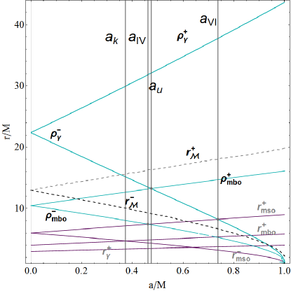
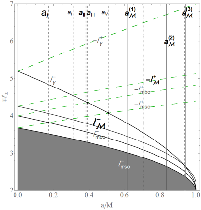
Figure 5: Upper: Complementary geodesic structure of the Kerr geometry: notable radii $\rho_{i}\equiv(\rho_{\mathrm{mbo}}^{\pm},\rho_{{\mathrm{\gamma}}}^{\pm})$ and $r_{\mathcal{M}}^{\pm}$. Bottom:fluid specific angular momentum $(\ell_{\mathrm{mbo}}^{\pm},\ell_{{\mathrm{\gamma}}}^{\pm},\ell_{\mathcal{M}}^{\pm})$.

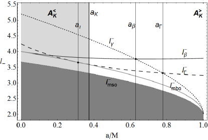
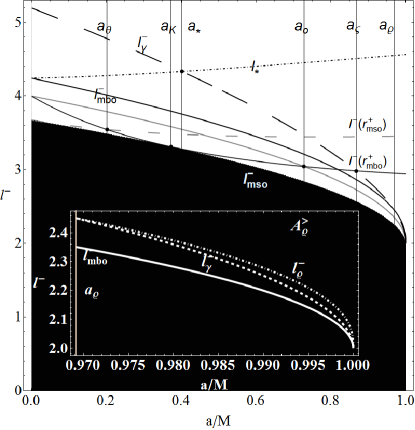
Figure 6: Some notable spacetime spin-mass ratios are also plotted, with remarkable specific anglar momentum with reference to Table 2, Fig. 13 and Table 6

IV On the energetics of $\ell$counterrotating accreting tori

We conclude the analysis with some notes on the energetics of the processes involving $\ell$counterrotating accreting tori. We concentrate on the specific example of the RAD accreting tori $\mathrm{C}_{\times}^{-}<\mathrm{C}_{\times}^{+}$ represented in Fig. 4 (a); this is a special case of the RADs, where the outer torus is counterrotating and the inner torus is corotating with respect to the central Kerr BH, and both tori are accreting. A further interesting aspect singling out this special RAD is the occurrence of a jet emission associated with each of the accreting toroid. Jet launching is associated to proto-jets in the RADs, studied in Pugliese & Stuchlík (2016, 2018a) and to accretion, because of the correlation of the inner accretion edge, $r_{\times}$, and the jet emission launch, $r_{J}$. In this regard we mention Fender (2001, 2009); Fender & Belloni (2004); Fender et al. (1998, 1999); Fender & Pooley (1998) for a detailed perspective of the possibility that highlights oscillation between the inner disk and jet in GRS 1915+105.

In the specific case considered in this section, where a double accretion occurs and double jets can be expected, it is also possible that the two jets associated to the RAD $\mathrm{C}_{\times}^{-}<\mathrm{C}^{-}<\mathrm{C}_{\times}^{+}$ are separated by a screening, corotating, and quiescent torus, located between the two lunching points: $\mathrm{C}_{\times}^{-}\leq r_{J}^{-}<\mathrm{C}^{-}<r_{J}^{+}\leq\mathrm{C}_{\times}^{+}$. The jets are correlated with the corotating inner shell, and the counterrotating outer shell. In this case, we can evaluate the separation between the two jet emission points and its variation with the SMBH spin $a/M$ as in Figs 8 and 7, identifying $r_{x}\approx r_{J}$. The maximal separation of the shell emission points is $(r_{mso}^{+}-r_{mbo}^{-})$, which is a spin $a/M$ depended quantity. We could also consider the variation of the cusp luminosity with the spin parameter $a/M$, quantifying this distance in relation to the accretion rates. We examine the tori and BH accretion rates, tori cusp luminosity, and enthalpy-flux, mass-flux, and thermal-energy carried at cusp, for a specific case where the RAD fluid angular momentum distribution, the tori masses and the BH spin $a/M$ are fixed. Finally, we comment the variation of these quantities in dependence on the BHs spin $a/M$.

In many models of SMBHs at high redshift, $z>6$, alternate accretion phases of the SMBHs evolution are considered as a succession of accretion episodes from accreting tori causing, eventually, a random seed-BH spinning-up or spinning-down. A sequence of interrupted super-Eddington accretion phases, combined with sub-Eddington phases can appear. (Note that a super-Eddington accretion can also imply a low efficiency mass-radiation conversion (Abramowicz & Fragile, 2013).) In the RAD frame the sub-Eddington phase may be associated to the presence of a screening, non accreting, corotating torus $\mathrm{C}^{-}$ in the system $\mathrm{C}_{\times}^{-}<\mathrm{C}^{-}<\mathrm{C}_{\times}^{+}$, the accretion from the outer torus would be absorbed partially by the torus $\mathrm{C}^{-}$. As a consequence of this, the efficiency of the RAD and its luminosity are not determined uniquely by the inner accreting torus, in fact our analysis falsifies this assumption because of the possibility of the screening effects. We limit here to consider a simple version of this problem, examining the accretion rates of tori and BHs for $\mathrm{C}_{\times}^{-}$ and $\mathrm{C}_{\times}^{+}$, in dependence on the parameter $a/M$ variation.

IV.1 Accretion conditions

We consider an inner corotating accreting torus and an outer counterrotating accreting torus where ($\mathbf{A}^{\pm}$, $\mathbf{B}^{\pm},\mathbf{S}^{\pm})$ accreting models are defined in the following way: $\mathbf{S}:\,\{r_{s}=r_{mbo},\,r_{\times}=r_{mso}\}$, $\mathbf{A}:\,\{r_{s}=r_{mbo},\,r_{\times}=\widehat{r}_{x}\}$, $\mathbf{B}:\,\{r_{s}=\widehat{r}_{s},\,r_{\times}=\widehat{r}_{x}\}$. In the example where the inner edge of the accreting tori $r_{\times}^{\pm}\approx r_{mbo}^{\pm}$, there is $W_{x}\equiv W(r_{\times})=\ln K_{\times}\approx 0$ (coincident with the limiting asymptotic value for very large $r/M$ of the P-W potential $W$). We define the accretion point $\widehat{r}_{x}(a)\equiv r_{mbo}+(r_{mso}-r_{mbo})/\alpha_{x}$ where the constant $\alpha^{-}_{x}\approx 3.900$, for corotating tori, and $\alpha^{+}_{x}\approx 6.76029$ for counterrotating tori, while $\widehat{r}_{s}(a)<\widehat{r}_{x}(a)=r_{mbo}+(\widehat{r}_{x}-r_{mbo})/2$. We illustrate spin dependence of these radii and the corresponding fluid specific angular momentum and the density parameter $K$ in Figures 7. For the double-accretion couple, the situation where $r_{J}\approx r_{\times}\approx r_{mbo}$ is a limit case occurring when the centrifugal component of the disk force balance tends to dominate the gravity and pressure force components in the torus. We give a preliminary evaluation of the center of maximum hydrostatic pressure in the tori as $r_{mso}^{\pm}<r_{cent}^{\pm}<\rho_{mbo}^{\pm}$, in Fig. 8.

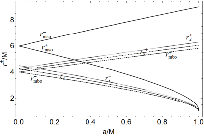
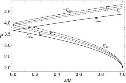
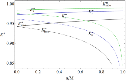
Figure 7: Radii $\{r_{mbo}^{\pm},r_{\times}^{\pm},r_{s}^{\pm},r_{mbo}^{\pm}\}$ (upper panel), fluid specific angular momenta $\{\ell_{mbo}^{\pm},\ell_{\times}^{\pm},\ell_{s}^{\pm},\ell_{mbo}^{\pm}\}$ (center panel), $K$-parameters $\{K_{mbo}^{\pm},K_{\times}^{\pm},K_{s}^{\pm},K_{mbo}^{\pm}\}$ (bottom panel) for models ($\mathbf{A}^{\pm}$, $\mathbf{B}^{\pm},\mathbf{S}^{\pm})$).

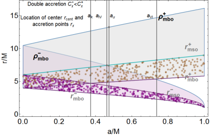
Figure 8: Double accretion $\mathrm{C}_{\times}^{-}<\mathrm{C}_{\times}^{+}$, location of tori centers $r_{cent}^{\pm}$ (dotted regions) and accretion points $r_{\times}^{\pm}$ (shaded regions) for corotating $(-)$ and counterrotating $(+)$ fluids. Location is according to Eqs (7). Constrains are used in the analysis of the models ($\mathbf{A}^{\pm}$, $\mathbf{B}^{\pm},\mathbf{S}^{\pm})$ in Figs 9. Crossing of the regions provides limits of the BH classification.

Figure 9: Evaluation of $\Psi$ and $\mathrm{N}$ in models ($\mathbf{A}^{\pm}$, $\mathbf{B}^{\pm},\mathbf{S}^{\pm})$ and dependence of $\Psi$ and $\Gamma$ on the SMBH spins $a/M$. Models ($\mathbf{A}^{\pm}$, $\mathbf{B}^{\pm},\mathbf{S}^{\pm})$ are constructed on the data on $r_{s},r_{\times}$ provided in Figs 7. This analysis refers to Sec. (IV), where $\kappa\equiv n+1$.

We start by considering two RAD tori constituted of polytropic fluids with pressure $p=K\varrho^{1+1/n}$. Within the formalism introduced in (Abramowicz & Fragile, 2013), we can estimate the mass-flux, the enthalpy-flux (evaluating also the temperature parameter), and the flux thickness. All these quantities can be written in general form $\Gamma(r_{x},r_{s},n)=q(n,K)(W_{s}-W_{x})^{d(n)}$, where $\{q(n,K),d(n)\}$, different for each torus, are functions of the polytropic index, $r_{x}$ is the cusp location and the inner edge of accreting disk while $r_{s}<r_{x}$ is related to thickness of the accreting matter flow and the P-W potential $W=\ln V_{eff}$. thus $W_{s}(W_{x})$ denotes, for a torus with fixed specific angular momentum $\ell$, the (constant) value of the P-W potential of the $p=$constant surface corresponding to radius $r_{s}$ ($r_{x}$).

Specifically the $\Gamma(r_{x},r_{s},n)$-quantities read:

$(\diamond)$ $\mathrm{{{Enthalpy-flux}}}=\mathcal{D}(n,K)(W_{s}-W)^{n+3/2}$

$(\diamond)$ $\mathrm{{{Mass-Flux}}}=\mathcal{C}(n,K)(W_{s}-W)^{n+1/2}$

$(\diamond)$ $\mathrm{E-L}=\mathcal{L}_{x}/\mathcal{L}=\mathcal{B}/\mathcal{A}(W_{s}-W_{x})/(\eta c^{2})$ which is the fraction of energy produced inside the flow and not radiated through the surface but swallowed by central SMBH.

$(\diamond)$ Efficiency $\eta\equiv\mathcal{L}/\dot{M}c^{2}$, $\mathcal{L}$ is the total luminosity, $\dot{M}$ is the total accretion rate, and for a stationary flow, $\dot{M}=\dot{M}_{x}$.

We examine also $\Pi$-quantities having general form $\Pi={\Gamma}(r_{x},r_{s},n)r_{x}/\Omega_{K}(r_{x})$; $\Omega_{K}(r_{x})$ is the Keplerian frequency of the accreting tori cusp $r_{x}$, where the pressure vanishes. Making explicit the polytropic index, there is

$(\bullet)$ the cusp luminosity

$$\mathcal{L}_{x}={\mathcal{B}(n,K)r_{x}(W_{s}-W_{x})^{n+2}}/{\Omega_{K}(r_{x})}$$ (10)

, measuring the rate of the thermal-energy carried at the cusp;

$(\bullet)$ the disk accretion rate $\dot{m}=\dot{M}/\dot{M}_{Edd}$,

$(\bullet)$ the mass flow rate through the cusp (i.e., mass loss accretion rate)

$$\dot{M}_{x}={\mathcal{A}(n,K)r_{x}(W_{s}-W_{x})^{n+1}}/{\Omega_{K}(r_{x})}$$ (11)

. In Figures 9 $\Psi_{*}^{\pm}\equiv\Gamma(r_{x},r_{s},n)/q(n,{K})$ for $\Gamma$-quantities and $\mathrm{N}_{*}^{\pm}={\Gamma}(r_{x},r_{s},n)r_{x}/q(n,K)\Omega_{K}(r_{x})$ for $\Pi$-quantities, for $\kappa\equiv n+1=4(n=3)$. (For more general discussion see also von Weizsäcker (1951); Lynden-Bell & Pringle (1974))

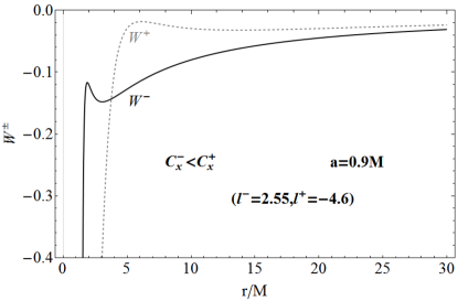
Figure 10: $W^{\pm}$-functions for models ($\mathbf{A}^{\pm}$, $\mathbf{B}^{\pm})$ for $\mathbf{BH}$ spin $a=0.9M$. $W^{+}$ ($W^{-}$) is the P-W potential for the counterrotating outer (corotating inner) torus of the RAD couple with specific angular momentum $\ell^{+}=-4.6$ ($\ell^{-}=2.55$), with cusp $\hat{r}_{x}^{+}$ ($\hat{r}_{x}^{-}$) used in models $\mathbf{A}^{+}$ and $\mathbf{B}^{+}$ ($\mathbf{A}^{-}$, $\mathbf{B}^{-}$).

IV.2 Time-dependent accretion

The stationarity of each RAD component, and therefore of the RAD agglomerate, has several relevant advantages but also some limitations. One significant advantage is that such set-up is able to provide very simple RAD configurations as initial data in GRHD and GRMHD dynamical analysis. However, stationarity also implies that for the dynamical analysis associated to the instability processes and, for example the emergence of the deterministic chaos occurring possibly after tori interactions, collision or double accretion, we need to extend our considerations beyond the stationary model, introducing the time-dependence and, eventually, explicit tori interaction terms. An interesting study would consist in the analysis of the BHs runaway instability to understand how the double accretion can affect this phenomenon. Here, we examine more simple general examples of situations where deterministic chaos might emerge, considering modified accretion rate laws (May, 1976). For this purpose we focus on the accretion rates of Figs 9 and explore the possibility that tori collision or screening effects, as described above, would provide a mechanism for interrupted phases of super-Eddington accretion as often considered in models of SMBHs evolution, altering $\dot{m}$ and $\dot{M}$ to include a time dependence. We explore the conditions under which the chaotic systems can emerge, starting from the initial configurations considered in Fig. 10, as in the models $\{\mathbf{A},\mathbf{B},\mathbf{S}\}$. In these models, we considered the relations between the accretion rates and the black hole spin $a/M$; we could assume this relation persists also in the time-dependent generalization. Accretion rates in the stationary systems investigated here are constant in time $t$, thus in general there is $\dot{m}=\dot{m}(0)\equiv\dot{m}_{0}$ and $\dot{M}=\dot{M}(0)\equiv\dot{M}_{0}$ for each torus at any $t\geq 0$. Depending on different constraints on evolutionary processes (analyzed at $t=$constant) in Pugliese & Stuchlík (2017), several scenarios had been envisaged for the double-accretion systems where, (1) the flow from the external torus decreases to stabilize, while the inner torus rate increases during the accretion process; (2) by changing initial conditions, the flow from the outer torus increases, the inner torus increases accretion rate and tori collision occurs; (3) in the third scenario, the accretion rate for the outer counterrotating torus increases, the inner torus decreases until accretion stops, and the torus stabilizes in a quiescent state. Finally, these (1) and (3) paths can be combined to give rise to some drying-feeding effects. These situations are widely discussed in Pugliese & Stuchlík (2017). The identification of a specific scenario asks to fix fluid conditions (GRHD or GRMHD dynamical models), depending on the initial model parameters $(\ell,K,a/M,r/M)$, where $r/M$ stands for the tori separation. In the stationary systems these are time-independent quantities.

In general, for small $t/M$, there is $\mathbb{\mathbf{(g)}}:\mathrm{{G}}[t;0]=\frac{1}{2}t^{2}G^{\prime\prime}(0)+tG^{\prime}(0)+G(0)$, in a proper range $\Delta t=t$, while $G(0)$ is evaluated and represented in Figs 9 where we explore the case $a=0.9M$.

The first case we consider in $\mathbb{\mathbf{(g)}}$ is the exponential growth with time of the tori and BH accretion rates. Fixing then accordingly $G^{\prime\prime}(0),G^{\prime}(0))$ and $G(0)$, we examine the law $\mathrm{\mathbf{(l_{1})}}:\mathrm{G}^{\pm}[t+1]=b^{\pm}\mathrm{G}^{\pm}[t]+h^{\pm}[t]$, thus $\mathrm{G}^{\pm}[t]=(e^{(b^{\pm}-1)t}[(b^{\pm}-1)\mathrm{G}^{\pm}[0]+h^{\pm}]-h^{\pm})({b^{\pm}-1})^{-1}$. The parameters $b^{\pm}$ give the rate of growing (decay) of the accretion rates. Parameter $h^{\pm}$ can be fixed considering the initial data $\mathrm{G}^{\pm}[0]$, thus $\mathrm{G}^{\pm}[t]=\mathrm{G}^{\pm}[0]e^{(b^{\pm}-1)t}$ for $h=0$. The relation, $\mathrm{G}^{\pm}_{t+1}=f(b^{\pm})\mathrm{G}^{\pm}_{t}$, where $f(b^{\pm})$ is a function of $b^{\pm}$ is however linear–as consequence of this there is no chaotic behavior.

Chaotic behavior appears in non-linear relations, as in the second case we consider, namely the polynomial form $\mathrm{\mathbf{(q_{1})}}:\mathrm{G}^{\pm}[t+1]=-b^{\pm}\mathrm{G}^{\pm}[t]^{2}+\mathrm{G}^{\pm}[t]+h^{\pm}$, leading to different tori evolutionary paths, including accretion rates decreasing in time. We constrain $b$ parameter (related to the rate of decreasing (or increasing) of the accretion rates) to the initial data. By setting $h=0$, we obtain a one-parameter model, with parameter $b$ related to the rapidity of the flow evolution and $\mathrm{G}^{\pm}[0]$. By considering the differential $\partial_{t}\mathrm{G}^{\pm}\approx\mathrm{G}^{\pm}[t+1]-\mathrm{G}^{\pm}[t]$ with $\mathrm{\mathbf{(q_{1})}}$, we obtain the general solution

$$\mathrm{G}=\frac{b-1-\beta\tan\left[\frac{\left(c_{1}+t\right)\beta}{2}\right]}{2b},\;\beta\equiv\sqrt{b(2-4h-b)-1},$$ (12)

where $c_{1}$ is fixed by $\mathrm{G}_{0}$ for each torus. We simplify the analysis with condition $h=0$, the general solution has then a simpler exponential behavior

$$\mathrm{G}=(1-b)\left[\frac{e^{(1-b)t}[b(\mathrm{G}_{0}-1)+1]}{\mathrm{G}_{0}}-b\right]^{-1},$$ (13)

where the rapidity depends on the parameter $(1-b)$; $b=1$ is then a limiting value we investigate below.

For small $t$, there is

$$\mathrm{G}\approx\mathrm{G}_{0}+t[1+b(\mathrm{G}_{0}-1)]\mathrm{G}_{0}[1+b(2\mathrm{G}_{0}-1)]+$$

$$\frac{1}{2}t^{2}\mathrm{G}_{0}[b(\mathrm{G}_{0}-1)+1][b(2\mathrm{G}_{0}-1)+1]+O\left(t^{3}\right).$$ (14)

It is easy to see that the rate is constant in time for $\mathrm{G}=\mathrm{G}_{0}=\frac{b-1}{b}$ or $b=(1-\mathrm{G}_{0})^{-1}$.

On the other hand, this situation occurs only when $b<0$ or $b>1$, which is satisfied for $a=0.9M$, while it is likely not satisfied for larger values of $a/M$. Eventually, for very large spin, a phase where $b<0$ could occur. Evolution in time is represented in Fig. 11 with data from Fig. 9. As expected, the study of the fixed points for the first cycle leads to $\mathrm{G}=(b-1)/b$ (for $b<0$ and $b>1$), with first derivative of $(\mathbf{\mathrm{q_{1}}})$ in this point being $(2-b)$, distinguishing the range of $b$ in $b>3$ or $b<3$ ($|2-b|>1$ or $|2-b|<1$ for stable equilibrium point). As clear from Figs 11, $\mathrm{G}$ decreases or increases in time depending on $b$: in one possibility we consider, the inner corotating torus decreases to $\mathrm{G}=0$ being thus a quiescent torus, while for the outer counterrotating torus the rate increases with time. Then we proceed with the analysis of the successive steps (cycles) for the neighborhood of the unstable points, namely the first cycle $G[t+1]$ as function of $G[t]$ (we assumed $t_{0}=0$), the second cycle for $G[t+2]$ as function of $G[t]$ up to $\upsilon$-cycle, for $G[t+\upsilon]$ as function of $G[t]$. The stability analysis for the second, third and fourth cycle is in Figs. 11 where the emergence of chaos for the outer counterrotating torus is demonstrated.

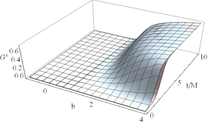
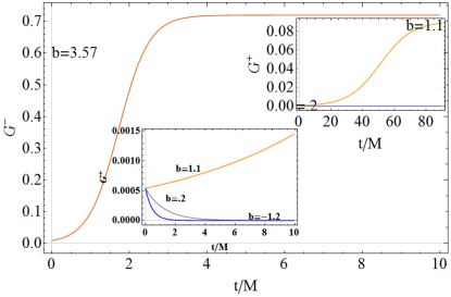
Figure 11: Upper Panel: $\mathrm{G}^{\pm}$ as function of $t/M$ and $b$ parameter for the dynamical solution of Sec. (IV). Initial data are for the accretion rates $\dot{M}^{+}[0]=0.00054$ for the outer counterrotating torus (red surface), and $\dot{M}^{-}[0]=0.00845$ for the inner corotating torus (blue surface), related to function $\Pi$ in Figs 9 for a=$0.9M$. For $b>2$ the rate generally increases with time towards a stable value (stationary hypothesis), for $b<1$ the rate may decrease with time according to the initial data. Bottom panel: $\mathrm{G}^{\pm}$ as function of $t/M$ for fixed values of $b$. Inside panels show the situation for $\mathrm{G}^{+}$ for different values of $b$. The increasing time profile of $\mathrm{G}^{-}$ is shown for $b=3.57$. The function $G^{-}$ is fast increasing, giving emergence of chaotic analysis studied in Figs 12.

V On the RAD instabilities and generalization of the RAD model

The RAD macrostructure is relevant for different aspects of the BH attractors and their host galactic environments, for example as explanation of the accretion rates of SMBHs at high redshift, or as model of screening tori, or also into the description of the QPO emission. The RAD hypothesis could play an important role also with regard to thick (outer) torus of gas and dust encircling the AGNs accretion disk (obscuring tori). On the other hand, current analysis of astrophysical BHs interacting with their environments suggests that the formation of multiple tori (from different accretion phases or fragmentation from an original disk and also galaxy interaction) is likely to occur Bogdán et al. (2018). Concerning RAD in their hosts, RAD proto-jet launch could be connected with AGNs very fast (almost speed of light) jets. (RAD accretion in a galaxy could emit radiative power outshining the host galaxy). Further analysis also suggests the possibility to detect structured proto-jets as sequences of jet-like configurations (or jet-bundles), constrained in spacings and relative fluids rotation. Below we outline some of most intriguing aspects of the RAD hypothesis which can have interesting implications

$\mathbf{(\bullet)}$ Our investigation suggests that, as expected, the BH spin distinguishes corotating from counterrotating tori by favoring generally the formation of corotating configurations, proto-jets and accreting tori, with respect to the counterrotating ones, according to the constraints provided on tori dimension ($K$-parameter), the specific angular momentum ($\ell$-parameter), and the BH dimensionless spin. This frame enters the wide field of investigations on the relevance of the counterrotating accreting tori, binding the situations where such tori can collide or double accretion can occur.

$\mathbf{(\bullet)}$ A further phenomenological application of the RAD is the connection between RADs seismology and the QPOs, the low and high frequency peaks in the power density spectra, which could be interpreted in the RAD frame as derived from the tori aggregate oscillation modes: the axis-symmetric and incompressible mode of each torus of the aggregate, variously associated in several studies with the QPO emergence (Montero et al., 2007), has to be combined with the peculiar modes arising by stratified structure of the RADs (Pugliese & Stuchlík, 2015). The RAD oscillations can also lead, eventually, to an alteration of the macrostructure elongations and spacings.

$\mathbf{(\bullet)}$ From the observational view–point, a RAD could be “disguised” as a single disk combing a complex mix of several properties. The RAD macrostructure can disrupt the usual “disk-model”–“disk geometry” correlation, especially as regards the assessment of the accretion rates. In fact, RAD matches the geometry of a geometrically thin disk with the specific characteristics of a geometrically thick disk, as the high accretion rates, in the frame of a stratified inner RAD structure, a differential relational law and a knobby, but axial-symmetric, RAD disk (envelope) surface (Pugliese & Stuchlík, 2015). RAD can therefore play an important part in the debate on the SMBHs origin. The episodic RAD accretion phases with super-Eddington accretion rates might be considered to explain the SMBHs origin from (intermediate or low mass) BH “seeds” of $10^{4}-10^{2}M_{\odot}$–(van Paradijs & Stollman, 1984; Stollman & van Paradijs, 1985). This issue applies to SMBHs formation and evolution at cosmological distances (Oka et al., 2017; Kawakatu & Ohsuga, 2011; Li, 2012; Volonteri et al., 2007; Volonteri, 2007, 2010; Allen et al., 2006). Long and continuous accretion episodes have been considered as origin of the BH masses, involving also a relevant spin-shift (particularly in elliptic galaxy hosts) or, vice versa, a series of small and random accretion episodes due to cloud accretion or also tidal disruption of a star (spiral galaxies), see for example Bonnell & Rice (2008). This situation can be clearly reflected by the RAD macrostructure. The internal structure of the RAD induces a peculiar internal dynamics, made up of tori interaction, the drying–feeding processes and screening effects Pugliese & Stuchlík (2017). Indeed, the RAD would be able to describe screening effects of X–ray emission (Marchesi et al., 2016; Gelli et al., 2007; Marchesi et al., 2017; Masini et al., 2016; DeGraf et al., 2017; Storchi-Bergmann et al., 2017) describing the screening tori as the inner torus of the RAD or the inter–torus located between two tori where the outer one of the couple is accreting towards the central attractor–see Eq. (8). This situation was restricted in Sec. III to some specific cases.

In this section we explore possible generalizations of the RAD, where different models are considered for the aggregate components. We have already pointed out that a part of the RAD impact in its galactic environment derives from the “macrostructure-level”, i.e., from the tori interaction in the RAD, being therefore in these aspects quite independent from the accretion disk model adopted for each component. In the following we consider the RAD symmetries exploring the relevance of the misaligned and warped tori within an agglomeration. Then we discuss the tori self- gravity influence in the emergence of the RAD instabilities, and the relevance of the self-gravity component of the toroidal disks with respect to the different contributions of the disk force balance. Finally we conclude this section examining briefly the main aspects of the magnetic field contributions in RAD instabilities.

V.1 Symmetries in RADs

This first realization or RAD model has been constructed considering agglomerated coplanar and axi-symmetric toroidal disks centered on a spinning BH. This situation could be seen as the final steady state of an original, more complex, environment constituted by an originally misaligned disk orbiting a central Kerr BH. There are indications to assume, at least in a first phase of formation, a torus misalignment with respect to the BH attractors arises, and a warped and tilted accreting torus occurs–see for example (Nelson & Papaloizou, 2000; Scheuer & Feiler, 1996; King et al., 2005; Liska et al., 2018; Stone et al., 2018; Doğan et al., 2015; Lodato & Pringle, 2006; Armitage & Natarajan, 1999; Fernández-López et al., 2017; Perego et al., 2009; Martin et al., 2009). The disk misalignment depends, however, significantly on the central BH spin. The dragging of frames, Lense-Thirring (L-T) effect, has a crucial influence on the morphology and equilibrium of an accretion disk and this has also a notable importance in the misalignment.

More generally, the description of this situation involves several aspects of the accretion disk physics. (1) Misaligned disks exploration faces aspects of the accretion disk formation after different processes: from a binary system, made up by a BH with a star companion or as formation from local matter of the BHs environments. Misaligned disks are especially expected orbiting BHs in binary systems where the BH spin axis is generally misaligned with the orbital plane of the companion star. Consequently, in the early ages of disk formation, the angular momentum of the infalling material from the BH companion to the forming torus, can be misaligned with respect to the binary orbital plane and the Kerr BH equatorial plane. Therefore, one may expect that the tori misalignment can provide description of the early phases of formation of the RAD multiple tori. As we describe below, this special situation can provide probable means to justify the origin of counterrotating tori of the RAD. (2) The warping and twisting of the disk depends on the disk composition, the viscosity, the presence of magnetic fields, and the frame-dragging (Bardeen–Petterson effect Bardeen & Petterson (1975)) and, in a binary system, the disk inclination with respect to the orbital plane of the star companion. (3) The probable final steady stage of an initially misaligned torus is expected as a coplanar, near–BH, accreting disk. This inner torus can be relatively small compared to the outer disk and the original torus. The outer part of such disk is aligned more slowly on the longer timescales. (4) Misalignment can also provide a ringed structure by creation of several tori from an original warped disk which splits after the warping. The initially inclined disk can twist because of the tidal effect of the star companion. The torus has therefore two distinct regions: an inner region, close to the central BH and an outer region, the farthest from the central attractor. The inner regions of the disks being located on the equatorial plane, while the outer regions are inclined because of the accretion from the companion.

For the RAD model, it is important to assess the time periods of the accretion from the companion star (companion accretion rate). The tori outer regions remain influenced by the differential precession of the tidal torques, following therefore the binary orbital plane. The disk region precesses around the axis parallel to the binary orbital axis. The torus inner regions, on the other hand, are affected by the differential precession due to the BH frame-dragging, and in turn this effects aligns the inner parts of the torus with the BH spin (Bardeen–Petterson effect). Consequently the torus finally becomes warped and twisted with an inner part aligned with the spin of the central Black hole. The disk will eventually reach a steady state, which is expected also from the process of continual matter feeding from the star companion. Noticeably it has been proved that when the disk outer regions are almost counter–enlightened, the disk can form a counterrotating torus with respect to the central BH.

Although probable in an early, transient, period of the attractor–accretion disk life, misaligned disks can have a considerable importance also in the RAD framework, in the jet–emission scheme related to the inner part of the accreting disk. Considering the torus regions partition, due to the binary precession and L-T effects, jets emitted in the inner torus region (inner-disk—jet correlation), would be aligned with the BH spin. A warped disk finally could be considered as the explanation for the correlation between AGN radio jets and the galaxy disk plane. This fact can have an influence also on the QPO emission. More precisely, the torque derived from the L-T effect has been related to the QPO emission in X-ray light–curves.

Magnetic fields are also able to condition the first phases of the disk formation, the galactic magnetic field could alter the structure of the accretion torus, influencing the disk initial inclination. (We note that the large–scale vertical magnetic field influences also the jets orientation). Furthermore, in presence of strong large-scale magnetic field there is a bending of the inner part of the disk and jets into partial alignment with the BH spin. However some studies have shown that the increase of disks masses (in RAD parametrization, this means a $K$-parameter increase) such inclination would disappear thus, under certain conditions, the disk inclination does not arise or turns finally to vanish.

Viscosity is a further aspect affecting the viscous disk misalignment, leading the inner disk regions aligned in the BH equatorial plane (Bardeen & Petterson, 1975). We can asses the impact of the viscosity in the viscous disk dynamics distinguishing a (warping) wave–like regime and a diffusive regime, depending on the Shakura & Sunyaev dimensionless viscosity parameter and the disk thickness. In fact, warps in the misaligned disks can diffuse on a viscous time–scale, and can also decay extremely rapidly as the differential precession combines with the viscosity. We can specify this mechanism, identifying in the disk a transition radius defining the point at which the disk specific angular momentum becomes aligned with the BH spin. This radius, depending on several factors of the disk model, has a role in the eventual fragmentation of the original disk into a multi-toroidal structure. Therefore, more generally, considering the balance of the tidal forces, the frame-.dragging and viscous effects, we can define the following three relevant radii: (i)The Lense–Thirring radius, $\mathrm{R}_{\mathbf{LT}}$, where Lense–Thirring precession and the effects due to the viscosity balances; (ii) The tidal radius, $\mathrm{R}_{\mathbf{tid}}$, where the tidal term balances the viscous term; (iii)The warp radius, $\mathrm{R}_{\mathbf{warp}}$, related to the rate of disk warping. Some models are expected to be warped in a region between $\mathrm{R}_{\mathbf{LT}}$ and $\mathrm{R}_{\mathbf{tid}}$, having a largest rate of warping at $\mathrm{R}_{\mathbf{warp}}$.

V.2 BHs and misaligned disks

In this article we have shown the importance of the spin–to–mass ratio of BHs in shaping the main morphological and stability characteristics of RADs. The impact of the BHs spin on the misaligned disks reflects in the Bardeen & Petterson effect. In the context of the misaligned disks, a BH warped torus evolves together with its attractor, changing its mass, the magnitude of its spin, and the spin orientation. It has been shown that a BH can align with the accretion disk outer part within a time–scale shorter than the accretion time-scale. However, for a geometrically thick disk considered here as model for a torus of the RAD agglomerate and associated to super-Eddington rates, alignment should occur at the mass accretion time–scale. On the other hand, the twisting of the accreting disk can enforce the internal dissipation as a mechanism which leads to increase of the accretion rate. We also note that jets can extract large amounts of BH rotational energy affecting also the disks structure; this holds particularly for a tilted torus, where jets can contribute to the alignment of the torus inner parts with the BH spin. Concerning the spin magnitude, it is generally expected that corotating disk accretion is associated to a BH spin–up, however, accreted material from counter-aligned accretion disks could induce a BH spin–down rather than a spin–up. There are further aspects to be considered to trace a more complete picture of the RAD instability process. For example, the presence of wind (particularly in the mass loss from accretion flow) is a further aspect of the tori physics which could be considered in relation to the effects of the double accretion phase typical of the RAD.

V.3 Tori self–gravity and RAD instabilities

The RAD stability has been discussed in Sec. II.2 and Sec. III. Then, as each torus of the aggregate is modeled by a geometrically thick disk, torus self-ravity may be relevant. However, we have also stressed that in some circumstances a torus component, especially the inner corotating RAD tori, can also be rather small, i.e., $K\gtrsim K_{\min}\equiv V_{eff}(r_{cent})$. In the RADs, tori self–gravity should have a great impact with respect to the concurrent effects in the force balance, such as the background curvature, the centrifugal effects, and the magnetic field contributions, especially in the largest tori, with large magnitude of the specific angular momentum $\ell$, located far from the central BH, and with large $K$-parameter. Among these tori we mention the counterrotating tori orbiting in the spacetimes of the faster spinning BH attractors.

It has be shown in other contexts that tori are unstable, if considered as self-gravitating systems; formation of $\ell$corotating pairs after fragmentation of an original seed disk can be one of the outcomes of this effect, similarly to the misaligned disks where however the torsion, typical of the binary systems, is at the origin of the original disk split. However, the newly formed outer torus always has, if it is part of a $\ell$corotating couple, a specific angular momentum greater (in magnitude) than the inner torus and at fixed angular momentum, and a disk in accretion reaches its maximum elongation (and dimension) with respect to the quiescent disk. Whether self–gravitating disks fragment, and the determination of the number and dimensions of the disk debris, depend on several parameters–tori masses with respect to attractor, and the rate of energy loss and cooling. Fragmentation, on the other hand, can provide a context in the galactic environment for stars and regular spiral structure waves formation (Shlosman & Begelman, 1987; Lodato, 2007; Shadmehri & Khajenab, 2006; Kubsch et al., 2016; Alexander et al., 2008; Ghasemnezhad & Abbassi, 2016; Abbassi et al., 2013; Anthony & Carlberg, 1988; Hunter, 1963; Bertin & Lodato, 2001, 1999; Woodward et al., 1994; Tohline & Hachisu, 1990; Shlosman & Begelman, 1989). Also, rotation of disks in the central part of various galaxies, for example NGC4258, shows a divergence from the Keplerian rotation law–(Herrnstein et al., 1998a, b). In the RAD scenario, one might consider the internal differential rotation due to the ringed structure, but other interpretations can involve the misalignment or the self–gravity of the disks. Nevertheless, especially in AGN disks, the presence of viscosity combines with self–gravity, affecting eventually the torus turbulence, modifying both accretion rates and the disk force balance, together with the angular momentum distributions. These factors reshape the angular momentum profile, obviously conditioning the stability of the disk. Furthermore, the induced internal waves would contribute to the transport of angular momentum in the accretion phase together with the eventual turbulence generated by the Balbus–Hawley mechanism (Balbus & Hawley, 1991).

It should also be said that if the self-gravity is combined with the L-T effect for the region of the disk closest to the central attractor, then this situation may lead to counter-rotation of the external part of the disk. Furthermore, runaway instability, typical of thick tori, can combine with the torus self-gravity, affecting the torus radial and vertical structure. Note that torus self-gravity implies a modification of the gravitational background that obviously influences the adjacent tori in the agglomerate. The oscillations of each toroid of the RAD will be a further factor of instability for the entire aggregate which combines with the disk self-gravity.

V.4 Magnetic field contribution in RAD instabilities

Magnetic fields are extremely relevant in the physics of accretion, altering the accretion phase. We specify that, although not considered here, magnetic fields have a significant role also in the jet emission and in the jet collimation. Above, we discussed the impact of the magnetic fields in several aspects of the formation of non–aligned disks. However, the influence of magnetic fields is varied and we report here some considerations in connection with the RAD stability.

RAD constituted by tori endowed with toroidal magnetic fields (relevant for geometrically thick disks and involved in dynamos processes) have been treated in Pugliese & Montani (2018), On the other hand, the case of a poloidal magnetic field in a more complex GRMHD-RAD model is planned for future investigation. We mention, concluding this section, some important aspects of the magnetic field in RAD tori in regards to the RAD equilibrium and the classification of the BH attractors. The analysis of the toroidal magnetic field case has shown the divergence with the purely HD case in the tori rotation law. However, the introduction of the magnetic field does not alter many of the main characteristics of RAD disks as the constraints on main seeds couples; the magnetic field rather combines with the constraints derived by the GRHD model. Moreover, the GRHD tori considered for the RAD are often used an initial configuration in the current GRMHD models (Porth et al., 2017; Abramowicz & Fragile, 2013). Therefore, we expect that a numerical integration of GRMHD-RAD should be set on the tori- attractor constraints provided by our investigation. Concerning the influence of magnetic fields in the tori and RAD stability, there are several recent studies focusing on the combined effects of the PP instability, the global non–axi–symmetric hydrodynamic Papaloizou–Pringle (PP) instability, and the magneto–rotational instability (MRI) due to the magnetic field and fluid differential rotation. Firstly, in general, MRI is most effective and fast in transport of angular momentum across the disk, and higher accretion rates were proved to occur in the magnetized models. (We remind that disks can be locally HD stable, according to Rayleigh criterion, but unstable for MHD local instability.) An extensive general discussion of the situation can be found in Pugliese & Montani (2018); Del Zanna et al. (2007); Wielgus et al. (2015); Das et al. (2017); Bugli et al. (2017). PP instability is associated to the formation of long–lasting, large–scale structures which have been also recently connected to the gravitational wave emission–see for example Kiuchi et al. (2011). A series of recent analyses shows that inclusion of a toroidal magnetic field could strongly affect, even with a sub–thermal magnetic field, the PPI. MRI can trigger predominant larger modes of oscillation (i.e. smaller length scales) with respect to PPI modes, altering therefore the equilibrium properties. More precisely, geometrically thick tori with a toroidal magnetic field develop the (3D) non-axi-symmetric MRI affecting the configuration on the dynamical timescales see Del Zanna et al. (2007); Wielgus et al. (2015); Das et al. (2017); Bugli et al. (2017). One of the possibilities is the suppression of the PPI by the MRI, or vice versa MRI and PPI can coexist depending on several parameters. Considering the RAD framework, the emergence of the MRI suggests an accentuation of the effects of the RAD own instabilities, discussed in Sec. II.2 to accent phenomena connected with energy release and matter impact.

VI Discussion and Concluding remarks

We investigated agglomerations of accreting coplanar tori (RADs) orbiting in the equatorial plane of a Kerr BH attractor as tracers of the Kerr SMBHs. The limit of the RAD constituted by one torus in accretion is also considered. This analysis eventually proves the existence of a strict correlation between the BH spin-mass ratio $a/M$, and the accretion tori featured by the RADs. Our findings resulted in the complete description of the RAD systems characterizing the central Kerr BHs in classes which are uniquely identifiable through the properties of the rotating tori of the agglomerate. Overview of the major features of the classes of spinning attractors has been discussed, according to the properties of the orbiting toroidal structures. Table 2 collects the main classes characteristics. More specifically, we developed a general classification of attractors and orbiting tori gathering together information on the Kerr BHs spin and their orbiting accreting tori in the RADs framework introduced in Pugliese & Montani (2015); Pugliese & Stuchlík (2015, 2016, 2017, 2018a). As consequence of this analysis, different issues related to the SMBH-RAD systems were addressed such as the identification of observable features of the toroidal agglomerates the indication of the associated BH classes according to their dimensionless spin. These classes associate a RAD to its central attractor, therefore they provide indication on the BH environments where it would be possible to observe a RAD. Eventually we addressed more explicitly the question whether there is a way to unambiguously identify the RAD aggregates through the specification of the RADs order, angular momentum distributions, the relative rotation of the toroids, toroid rotations with respect to the attractor, and internal dynamics of the SMBHs (the spin-mass ratio). This investigation serves to different purposes: to envisage an accretion disk–SMBH correlation in the RADs scenario, or in the limiting case of one orbiting torus, and to provide an indication of the possible attractor-disk candidates to look for observational evidences of RADs. This work supplies the most comprehensive reference template of BH-accretion tori correlation, which can be also used an a strictly constrained set of the initial configurations for the development of a fully general relativistic dynamical GRMHD simulation for the SMBH-RAD system–see for example Porth et al. (2017); Abramowicz & Fragile (2013).

Our analysis is conducted by numerical integration of the hydrodynamic equations for multiple tori with fixed boundary conditions for each configuration of the set–see Figs 4. Parallel to this analysis we carefully explored the ranges of fluid specific angular momentum and $K$-parameters, drawing then the constraints for the radii $(r_{cent},r_{\times})$ and $(r_{in},r_{out},r_{coll})$–see also Pugliese & Stuchlík (2016, 2017, 2018a). It is clear that the construction of the aggregates relies essentially on the boundary conditions imposed on the function (15) (the Heaviside functions). We used the studies of Pugliese & Stuchlík (2016, 2018a), which fix the location of the accretion torus edges in the spacetime regions confined by marginally bound, marginally stable and marginally circular (photon) orbits. This setup turns to be very important for the analysis of the RAD oscillations emerging as perturbations of tori and the boundary conditions (Pugliese & Stuchlík, 2015). The RAD model encloses a huge amount of possibilities to be investigated, having a large number of cases even in the simple three parameters model considered here (the specific angular momentum $\ell$, the $K$ parameter and the attractor spin-mass ratio). Interestingly, this investigation enlightened also the importance of the dimensionless quantities $\ell/a$, $r_{cent}/a$ and $r_{in}/a$, while a deeper analysis of the BHs-accretion tori connection in this special parametrization is reserved for a planned future work. We consider these configurations using a seed to generate a general sequence of the RAD tori, starting from one of the four germs $\textbf{()}_{\pm}>\textbf{()}_{\pm}$ (the $\ell$corotating couples) or $\textbf{()}_{\pm}>\textbf{()}_{\mp}$ (the $\ell$counterrotating couples) respectively–Figs 1.

Focusing here on the central objects around which these configurations may orbit, and considering different properties of the configurations, we drawn a detailed classification of the attractors in $17$ general classes singled by the their BHs spin-mass ratios in the entire range $0\leq a\leq M$, including the Schwarzschild static solution and the extreme Kerr solution. As expected, this classification tends to strongly differentiate fast spinning attractors and slow spinning ones. Major differences are highlighted for two classes of attractors, with spin $0<a\leq 0.47M$ and $a>0.47M$ respectively. The static case, represented by the Schwarzschild solution, was considered separately. A further relevant aspect of this analysis is that the BH classes often intersect–see Fig. 13. Importantly we have taken into account the RAD stability properties in the construction of the classes of attractors. The main aggregate instabilities are mainly driven by two families of processes: (1) Collisions between accreting or non-accreting tori, and (2) RAD instability following the accretion phase of one torus of the aggregate (Pugliese & Stuchlík, 2015, 2017).

A double accretion can be observed only in a couple $\mathrm{C}_{\times}^{-}<\mathrm{C}_{\times}^{+}$ (es Fig. 4), around all Kerr BHs ($a\neq 0$). Moreover, in the RAD scenario, the maximum number of accreting tori orbiting around one central Kerr SMBH is $n=2$. This opens up important potential observations encouraging also a review of the current interpretation of the accretion data by considering a RAD framework. In fact, the ringed structure can be effectively disguised as a geometrically thin, axi-symmetric disk centered on the equatorial plane of the Kerr SMBH with interrupted phases of super-Eddington accretions and a very rich inner dynamics with jet emission featuring also inter-tori, proto-shell, jet emission. The presence of an inner torus can also enter as a new unexpected ingredient in the accretion-jet puzzle–see also Lee et al. (2017b). Therefore, in Table 2 we also consider the possibility of launch of proto-jet configurations in the RADs. This situation however, has been deeply analyzed in Pugliese & Stuchlík (2016, 2018a). We have shown an important restriction on any screening effect from an inner torus of an aggregate. Screened X-ray emission by some “bubbles” of material are currently studied in many processes-(Gelli et al., 2007; Masini et al., 2016; DeGraf et al., 2017; Storchi-Bergmann et al., 2017; Ricci et al., 2017b; Almeida & Ricci, 2017; Marchesi et al., 2016, 2017). Then, particularly some AGNs have been proved to be obscured according to the X-ray spectral emission (Marchesi et al., 2016, 2017); several analyses also suggest that obscuration in optical and X-ray emission profile may be due to different phenomena, caused by dust materials surrounding the inner part of the galactic nuclei. So far these (free) dust materials were almost always supposed to be randomly distributed around the central BH and, depending on the gas density, the light emitted during the growth could be absorbed in the optic as in the X-ray electromagnetic band, distinguishing AGN as obscured, not obscured, or much obscured (or Compton thick). We here explicitly claim for an analysis of this obscuration assuming a RAD scenario, therefore considering the inner corotating, accreting or quiescent torus in accordance with the analysis in Sec. III, and with the constraints imposed by the spin of the central SMBHs. Such RADs are very much constrained so that they cannot be randomly distributed neither assumed to exist independently on the evolution of the SMBH itself–see also Pugliese & Stuchlík (2017, 2018a). We believe this change of paradigm may have a huge impact on the current scheme adopted to explain the obscuration. To be more precise, screening tori may only exist as corotating fluids in particular BH classes and under specific restrictions on the specific angular momentum. These tori can be accreting onto the central BH or quiescent– see also Pugliese & Stuchlík (2017, 2018a). A “screening” corotating, non-accreting, torus between the two accreting tori can be observed only as $\,\mathrm{C}_{\times}^{-}<\mathrm{C}^{-}<...<\mathrm{C}_{\times}^{+}$ for any Kerr attractor having spin $a\neq 0$. These special tori are expected to be relatively small compared to the outer tori of the RAD agglomerate. A further case is where the inner corotating or counterrotating (for BHs with $a<0.46M$) accreting torus of the RAD is “obscured” by an outer screening and quiescent torus. As seen in Table 2, a counterrotating accreting torus with an outer corotating torus towards the accretion (i.e. a $\mathrm{C}^{-}_{1}$ torus having specific angular momentum $\ell\in\mathbf{L1}^{-}$), can be observed only as a $\mathrm{C}_{\times}^{+}<\mathrm{C}_{1}^{-}$ aggregate, and orbiting around slow spinning SMBHs with spin $a<0.46M$. In the BH classification, we have also included very fast spinning SMBHs with $a>a_{1}$, which are characterized by the possibility that corotating (screening, accreting) tori can be orbiting in the ergoregion. This aspect, also mentioned in Pugliese & Montani (2015); Pugliese & Quevedo (2015); Pugliese & Stuchlík (2015, 2017, 2016), is an interesting consequence of the frame dragging.

More generally, we expect RAD to be a relevant feature of the faster-spinning SMBHs. Specifically the $\ell$corotating RADs are favored features of slow attractors $(a\lesssim 0.45M)$, while around faster spinning attractors, $\ell$counterrotating RADs would be most expected. Generally, in the spacetimes of the slower rotating BHs, tori collision appear more probably. This episode may be followed by the collisional energy release and, eventually, tori merging and accreting onto the central BH–Pugliese & Stuchlík (2018a). For the slow spinning BHs, with dimensionless spins $a/M$ close to the lower limit of the static attractors, any RAD tori couple has to be considered as an $\ell$corotating couple, independently of the relative rotation of the tori, i.e., although the tori of the aggregate can have alternate spin, eg. $(0,+,-)$ or $(0,-,+)$, according to the notation introduced in Fig. 1, their properties considered for RAD structure, are entirely analogue to the $\ell$corotating case in a Kerr spacetime. Moreover, in the Schwarzschild spacetime, double accretion or obscuration is not possible. On the other hand, very fast-spinning SMBHs $(a\approx M)$, would favor the formation of $\ell$counterrotating tori which are also largely separated in the RAD. This holds particularly for the couples $\textbf{()}^{-}<\textbf{()}^{+}$, where a double accretion phase occurs. Instead, the seed having an inner counterrotating torus in accretion with an outer corotating torus is favored only in the early phases of formation of the outer torus, for fast-spinning SMBH, while in Schwarzschild spacetime such a couple can be always observed–(Pugliese & Stuchlík, 2017).

Kerr SMBH attractors are significant environments for the RAD observation. In fact, SMBHs determine certainly strong curvature effects having ultimately a major influence in the determination of the constraints in (15). Then, as shown in Pugliese & Stuchlík (2017) and then discussed in Pugliese & Stuchlík (2018a), very massive BHs would prevent the emergence of tori collision. Note also that the space-scales are here in units of the SMBH mass; for example the maximum spacing $\bar{\lambda}$ considered for two accreting tori is $\bar{\lambda}\approx 8M$ in the case of nearly extreme BHs. To realize the significance of this we should note that the spacing parameter $\bar{\lambda}$ between two tori regulates in fact the possibility of tori collision. The unstable phases of the aggregate, on one hand, could undermine the survival of the ringed structure, eventually leading to the formation of a single disk. On the other hand, the RAD unstable phases constitute environment for set of interesting phenomena– see Pugliese & Stuchlík (2017). It is possible that a RAD represents a final steady state of life of an attractor-disk system originating as extended disk misaligned with the BH axis; this hypothesis stands as particularly promising for the very massive BH attractors in AGNs, as demonstrated in Sec. V–see also Nelson & Papaloizou (2000); Scheuer & Feiler (1996); King et al. (2005); Liska et al. (2018); Stone et al. (2018); Doğan et al. (2015); Lodato & Pringle (2006); Armitage & Natarajan (1999); Fernández-López et al. (2017); Perego et al. (2009); Martin et al. (2009).

VI.1 Relevance of the RADs in the AGN environments

It is clear that a SMBH is rarely an isolated BH, but rather a living object in the host galaxy cores interacting with its environment and subjected to several evolutionary phases, where its mass and spin will often change during different stages of the BH life. The SMBHs intercept the stellar population and dust of their galactic host and vice versa SMBHs remix, the matter and radiation content of the galactic environment. Suffering from galaxy collisions, the interaction between the BH and the galaxy environment ends in changes of the BH spacetime which is initially considered as “frozen background”. A non-isolated BH background can change following a spin-down or a spin-up process (Abramowicz et al., 1983, 1998; Rezzolla et al., 2003; Font & Daigne, 2002a; Hamersky & Karas, 2013; Adamek & Stuchlik, 2013; Korobkin et al., 2013). This clearly should lead to a BH shift from one class of our classification to another, and to a change of the equilibrium conditions of the RADs. Toroidal structures might be formed as remnants of several accretion regimes occurred in various phases of the BH life (Alig et al., 2013; Lovelace & Chou, 1996; Lovelace et al., 2014; Volonteri et al., 2003a; Carmona-Loaiza et al., 2015; Dyda et al., 2015) Therefore, the analysis considered here can be significant for the resolution of the so called mass problem for SMBHs in AGNs. We can consider accretion in long and continuous accretion episodes, arising due to merging involving a large spin-shift or, vice versa, sequences of small and random accretion episodes, being advocated for the formation of the SMBHs. The RAD internal dynamics has several inter-disk effects including double accretion processes, screening effects, and tori collisions. These situations clearly represent mechanisms for the mass growth of the SMBHs. It is clear that many aspects of the physics of SMBHs and their host galaxies would be altered by the relevance of the RAD model in support of the hypothesis of a more complex BH-accretion disk system, than is commonly considered.

In Sec. V we also examined the impact of the RAD scenario, regarding, more widely, future generalizations of the tori aggregate model to consider misaligned tori and, more generally, diverse accretion disk models. It should be also stressed that, although the current theoretical analysis conceives on a large variety of accretion models, with a diversified parametrization and disk shape (depending on disk optically depth, the geometric thickness, luminosity…), there are some general constraints that extended matter orbiting configurations must abide on the curved spacetimes—Abramowicz & Fragile (2013). This is an important feature of SMBH accretion disks validating also the relevance of the RAD model. However, accreting disk models are generally associated to specific characteristics of their BH attractors and especially their mass range(Abramowicz & Fragile, 2013). The geometrically thick disks, which were adopted here as aggregate components, are governed by the gravitational forces predominant with respect to other possible components of the force balance, and they are therefore associated to SMBHs spacetimes where the curvature effects and the fluid rotation are significant in the determination of the toroidal equilibrium and morphology.

VI.2 Phenomenology

RAD phenomenology is significant for the high energy phenomena related to accretion onto SMBHs in AGNs which could be observed in their X-ray emission. RAD framework also includes the jet launch with an interesting and intricate shell structure. These structures then fit into the more broad discussion on the role and significance of open surfaces in relation to (matter) jets emission and collimation, as well as jet-accretion correlation–see Kozlowski et al. (1978); Sadowski et al. (2016); Lasota et. al. (2016); Lyutikov (2009); Madau (1988); Sikora (1981). Among the other phenomenological application of these studies, there is a possible connection between RADs seismology and QPOs–low and high frequency peaks in the power density spectra–see also Ingram et al. (2016). The pattern of the possible oscillation modes of the tori aggregate has been provided and related to the evolution of instabilities in RADin Pugliese & Stuchlík (2015); Stuchlík et al. (2013). Missions like XMM-Newton or RXTE, NuSTAR (Nuclear Spectroscopic Telescope Array) are on the verge of these studies–see also Mossoux et al. (2014); Gelli et al. (2007) and Gandhi et al. (2017); Masini et al. (2016); Harrison (2013). The current status of observational mission and the potentialities in the next future provide certainly an increasingly high degree of details with which we can look at BHs and accretion disk morphology. The results outlined here thus are directly comparable with the current data and encouraging us to apply already these results for a re-interpretation of the current data analysis set up which is almost unanimously based on the scenario of BH one-accretion disk system – see for example Lee et al. (2017a, b). Possible evidence of the existence of the ringed accretion disk can be inferred from the study of the optical properties of the ringed-like structures (Karas & Sochora, 2010; Sochora et al., 2011; Stuchlík & Schee, 2012, 2010). Concerning the RAD optical appearance we expect that tori emanating radiation would be distorted into a belt-like configuration because of the curvature effects of the Kerr geometry. (Then the Lense–Thirring effect becomes clearly more important for corotating tori approaching the BH). This aspect will be considered in planned future investigation. We expect that optical phenomena could reflect the BH classification as they differentiate between corotating and counter-rotating tori in dependence of the BH dimensionless spin. Optical properties depend also on the geometrical thickness of the disk and the presence of a disk atmosphere (some accretion disks atmospheres can show similarity with the upper main sequence stars, where magnetic fields and winds appear (Weber & Davis, 1967). The analysis of the optical appearance of the thick accretion disk is also based on the model of hot coronae above the surfaces of accretion disks and a hot coronal layer implied in the emission profile– (Stalevski et al., 2012; Fuerst & Wu, 2007; Stuchlík & Schee, 2010, 2012; Schee & Stuchlík, 2009). BH RAD model may be revealed by future X-ray spectroscopy, from the study of excesses on the shape of the relativistically broadened spectral line profile, related to a sort of rings model which may be adapted as a special case of the RADs. Specifically, in Karas & Sochora (2010) extremal energy shifts of radiation from a ring near a rotating BH were particularly studied: radiation from a narrow circular ring shows a double-horn profile with photons having energy around the maximum or minimum of the range (see also Schee & Stuchlík (2009)). This energy span of spectral lines is a function of the observer’s viewing angle, the BH spin and the ring radius. Accordingly, the ringed disks may be revealed thought detailed spectroscopy of the spectral line wings, claiming for observation and data re-analysis in this framework, especially in relation with the BH classes considered here.

VI.3 RAD phenomenology and future perspectives for the RAD extensions

On one side, the possibility of more orbiting tori opens new perspectives of enriched accretion phenomenology connected to the RAD structure and its own internal dynamics. RAD typical effects as the double accretion phase or the presence of screening tori which are located between the BH and the accreting torus, or tori between two accreting RAD tori, the presence of AGN obscuring torus, are proved to be expected in specific contexts and under precise conditions on the tori and the central BH attractor. In this analysis we present limits indicating the parameter ranges where these situations occur. On the other side, in the RAD frame, we pose rather narrow constraints for different ad hoc models of several accretion processes which are currently considered, ruling out many of the assumptions considered so far on screening and obscuring phenomena. Those limits and some main indications on RAD observation are given below. This work provides a new scenario for the data interpretation which has been until now essentially framed into the single axi-symmetric, corotating, accretion disk model. Screening and obscuring tori in accretion processes are essentially positioned ad hoc in order to fit the observations and models. It is very likely that at least in the initial phases of the RAD formation, ringed structures may appear, and we explicitly call for a review of the analyses carried out so far in the simplest scenario of one torus model, shifting this classic setup to the model of orbiting RAD axi-symmetric structures including the counterrotating tori. Indeed, the predictions implied by the adoption of a RAD system fit some features of the accretion disk physics which puzzle the theoretical grounds of one class of accreting model, for example the geometrically thick tori with some features proper of geometrically thin disks.

A further important aspect in this regard stands in the fact that a RAD could have been disguised so far as one geometrically thin disk; in Pugliese & Stuchlík (2015) it has been proved that RAD can be treated as a geometrically thin disk blending with distinctive features of geometrically thick torus as super-Eddington luminosity (high accretion rates). This situation can fit a particular hypothesis made to justify the masses of SMBHs located in high redshift galaxies. Concerning the possibility of screening tori we proved that such tori must be corotating and screening effects could be possible only if the outer accreting disk is counterrotating, but this in fact rules out several of the models currently considered in the screened accretion. According to our analysis screening effects are likely to be observed around high spin BHs–precise limits and constraints are in Table (2). Further constraints on thickness and extension on the equatorial plane of the RAD, relevant to set power spectra obscuration follow, from more detailed analysis in Table (2). Those constraints will emerge as distinctive features of the emission spectra.

Most interestingly a screening effect may happen in the occurrence of a double accretion phase as in Fig. (4)-(a). The possibility of a double accretion from an $\ell$counterrotating couple is a new feature firstly presented in the RAD, we clamor for attention on the scientific community to focus on observations on high masses and high spin Kerr black hole where pieces of evidence of this phenomenon should be found. Besides we proved that no more then two accreting tori can be observed. The detection of a double accretion phase (associated to a double shell of jet emission) would imply the presence of an outer counterrotating accreting torus and an inner corotating one, the central BH is not screened. Vice versa, a quiescent corotating torus, screening the outer retrograde accretion, and the inner prograde one are possible. Such inert screening tori must be relatively small configurations. The analysis of the RAD characteristics which could be extracted from the spectrum emission or accretion rates/luminosity analysis, Pugliese & Stuchlík (2018a), may be used to locate the RAD in one of the attractor class of Table (2), thus identifying the central BH attractor. Spectra, for example from X-ray emission, would show evidence of the RAD spacing. Note that the distance in spin boundaries of the SMBHs classes can be very close, also up to $10^{-2}M$, this means that we can distinguish, considering RAD features, a spin range $\Delta a\approx 10^{-2}M$, depending on the constraints provided on the accretions properties. It should be noted that a large part of the accretion disk analysis is actually dealing mainly with corotating disks, our RAD analysis provides more precise insight on the physics connected with counterrotating tori.

Screening effects are possible only in the case of accreting counterrotating tori, this implies that the current analysis using a screening torus must take into account the fact that the outer torus, in the BH-screening torus-accreting torus system, is counterrotating. This is a strong restriction in the analysis of retrograde disks. On the other hand, if there is a system with a screening torus and an obscuring one, this situation implies that the BH spin has to be relatively small $a\lessapprox 0.46M$. Most importantly a corotating torus cannot be screened to the BH, i.e., no screening effect from axi-symmetric inner torus can be set–this means that many screening models are effectively ruled out.

A further interesting aspect is constituted by jet emission in RADs. RADs are related to jet emission in two different ways. Firstly, each toroid considered as RAD component allows open funnels, proto-jets, occurring when the centrifugal component in the disk force balance is strong enough to push matter along the vertical direction along the BH axis. Jet for retrograde tori is another interesting feature. We considered these open solutions too in the set-up of the attractor classifications, although a focused investigation of these are especially in Pugliese & Stuchlík (2016, 2018a, 2018a). Secondly, as jets are expected to be correlated to accretion and especially to the inner part of an accreting disk, the dynamical picture featuring more accreting tori, up to maximum of two $\ell$counterrotating accreting tori, including the possibility of screening and obscuring tori, is certainly an interesting perspective in the context of jet emission. We proved that there can be up to two jets (no proto-jets), i.e., double shell of jets. According to constraints on the double accreting phase, the outer jet being correlated to the outer retrograde RAD torus, and the inner jet from the inner corotating, accreting torus. Constraints on spacing and tori dimensions are set according to SMBH spin and details on these constraints are presented in Table (2). Spacing between the tori will reflect in the jets separations.

The change of BH spins will reflect in change of the spacetime and other features of jet emission. In this context, it is proper to stress that characteristic RAD features in accreting processes, such as screening and obscuring tori act also in regard of the jet emission, the presence of inert materials will affect the energy release, the jet launching and collimation. Small corotating tori will be located eventually between two accreting tori and inside the double jet shall, while in the case of one jet correlated to a counterrotating accreting torus, the BH-jet system, can be possibly characterized by an inner, screening, corotating torus. It is then crucial to establish possible RAD evolutions following the occurrence of the instability processes in the structure.

Constraints on RAD evolution have been discussed more extensively in Pugliese & Stuchlík (2017, 2018a). Generally, the situation after tori collision emergence, or accretion between two tori, with matter impacting from one torus to another, can result also in the destruction of the RAD, i.e. formation of one torus after tori merging. Evolution paths in these models were discussed in Pugliese & Stuchlík (2017), energy release associated to the collision and accretion phases including the evaluation of the torus cusp luminosity and accretion rates are examined in Pugliese & Stuchlík (2018a), where evolution is also discussed in context of energy release in RAD.

We can say that one possibility is the merging after accretion of the outer counterrotating torus of a couple or collision with one inert torus or during the double accretion phase; in all these cases there will be a modification of the stability properties of each involved torus, according to a variation of the parameters range, for matter supply from the outer accreting counterrotating torus, followed by an alteration of the fluid specific angular momentum and an increase of the $K$-parameter, reflecting change in density and tori dimension. Such phenomenon has to be considered, focusing on a more accurate prescription of the torus inner dynamics.

The possibility that the accretion or collision may in fact not lead to the destruction of the RAD inner structure, but rather to a sequence of instability processes (accretion phases) involving an inner torus has also been discussed. Concerning RAD evolution, it must be said that the oscillation modes of each toroidal component, will be combined together in the ringed structures to reflect the QPOs phenomenon–see discussion in Pugliese & Stuchlík (2015) for the RADs perturbation. One can assume oscillations of an individual torus of the RAD system, and possible excitation of tori oscillation by external influence, e.g, due to original oscillation of the first oscillating torus. The resonance models of the epicyclic frequencies could give relevant explanation of double peak QPOs. Such double QPOs are recently directly observed in AGNs (see Carpano & Jin (2018)) and they might be directly linked to the RAD systems, giving independent estimates of the mass and spin of the Kerr SMBH.

Finally, there are possible relevant extensions of the RAD model to be considered, according to the specific frame where the aggregate hypothesis may be applied. There are two main classes of model generalizations, the first involving a change in each aggregate component, for example in Pugliese & Montani (2018) magnetized RADs have been considered. Secondly, assumptions of RAD entire structure may be modified, particularly on regards of the aggregate symmetries. We discussed the relevance of tori misalignment in RADs in several parts of this work. Considering the different properties of in-falling matter from several companions during the accretion processes into the Kerr black hole, a tori misalignment is highly expected at least in the early phases of formation of the RADs. The presence of initial misalignment will lead also to a change of the entire BH-disk system inducing a variation of the BHs properties due to modifications of the spin magnitude and orientation.

The BH-RAD tori considered here might be seen as the final state of this complex scenario. In fact in several cases the final ending of the BH- misaligned tori dynamics results in equatorial disks. Wind and jet emission can be present in RADs, showing a very complicated behavior. This might possibly lead to non linear dynamics, and as a consequence of this, the RAD system may be subjected to deterministic chaos (e.g. May (1976)). Moreover, toroidal components of the RAD can exchange matter and angular momentum leading to different effects, this situation has been discussed in an evolutionary scenario in Pugliese & Stuchlík (2017): a possibility includes “drying-feeding” effects or evolutionary loops among tori of a RAD couple as described in Pugliese & Stuchlík (2017). Another possibility in this two-steps exchange of angular momentum between tori, is the excitation of oscillations which could eventually be observed as it occurs in the matter and angular momentum exchanges in certain class of binary stars. This behavior in general could be connected with the quasi-periodic or chaotic oscillations of the RADs. We shall deepen this aspect of the RAD dynamics and the model generalizations in future works. Particularly inclined tori will be set first in the simplest case of the spherically symmetric background of the Schwarzschild black hole and then slow rotating spacetimes will be analyzed. The ranges of spin variation in the slow regime will be located considering also the limits provided in the SMBHs classes provided of Table (2). A further extension on the model affecting tori symmetries is for the warped disk analysis where the tori warping will be included. Then in binary BHs systems (BBHs), BHs spins are usually not aligned (Moran, 2008), a complex RAD related problem is considering BBHs with two mini-disks and a circumbinary disks, with not aligned BHs spins.

Appendix A Notes on significant spin-mass ratios $a/M$

In this Appendix, we list further relevant limiting values of the Kerr BH spin, discussing the main features of the BHs in relation to the RAD toroidal components. We refer to Table 4 and Table 3. Moreover, Table 5 lists some general properties of the tori couples, some of these were discussed in Sec. III.

Table 3: Classes of attractors. Kerr BH spin regulating the magnitude of ratio $\ell_{i}/\ell_{o}$ for a seed of orbiting tori, in a defined regions of $(\ell-a)$ plane as in Fig. 3. Relations between the range of variation of the fluid specific angular momentum having relevance in the collisional problems. Arrows are in accordance to the decreasing spin (left column) or increasing spin (right column), starting from the initial spin in one column of the considered range of spin and ended by a second arrow of the other column.

Classes of attractors	down-to-top	Decreasing BH spins	top-to-down	Increasing BH spins
${{a_{I}}}\equiv 0.172564M:-\ell_{\mathrm{mso}}^{+}=\ell_{\mathrm{mbo}}^{-}$	$\uparrow$	$|\mathbf{L1}^{+}|\subset(\mathbf{L2}^{-}\cup\mathbf{L1}^{-})$	$\downarrow$	$|\mathbf{L1}^{+}|\subset\mathbf{L2}^{-},\;|\mathbf{Li}^{+}|>\mathbf{L1}^{-}$
${a_{III}}\equiv 0.390781M:\ell_{\gamma}^{-}=-\ell_{\mathrm{mbo}}^{+}$	$\uparrow$	$|\mathbf{L1}^{+}|\subset\mathbf{L2}^{-}$	$\downarrow$	$|\mathbf{L1}^{+}|\cap\mathbf{L2}^{-}\neq\emptyset,\;|\mathbf{L1}^{+}|<\mathbf{L2}^{-}$
${a_{V}}\approx 0.5089M:-\ell_{\mathrm{mso}}^{+}=\ell_{\gamma}^{-}$	$\uparrow$	$|\mathbf{L1}^{+}|\cap\mathbf{L2}^{-}\neq\emptyset,\;|\mathbf{L1}^{+}|<\mathbf{L2}^{-}$	$\downarrow$	$|\mathbf{L1}^{+}|\cap\mathbf{L2}^{-}=\emptyset$, $|\mathbf{L1}^{+}|>!\mathbf{L2}^{-}$

Table 4: Classes of Kerr attractors. For a spin value $a_{\bullet}$, the classes $\mathbf{A}_{\bullet}^{\lessgtr}$ stand for the ranges $0\leq a<a_{\bullet}$ and $a_{\bullet}<a\leq M$ respectively. Definition of angular momenta $({\ell}_{*},{\ell}_{\varrho}^{\pm},{\ell}_{\beta}^{-},\ell_{\Gamma}^{-},\ell_{\mu}^{-},\ell_{q}^{-})$ are in Table 6– see also Table 2.

SMBHs Spins		SMBHs Spins
$a_{\theta}=0.201697M\in]a_{I},a_{\iota}[:$	$\ell_{\mathrm{mso}}^{-}=\ell^{-}(r_{\mathrm{mbo}}^{+})$ and $r_{\mathrm{mso}}^{+}=r_{cent}^{1^{-}}$, $r_{\mathrm{mbo}}^{+}=r_{\times}^{1^{-}}$	$a_{II}=0.382542M\in]a_{K},a_{III}[:$	$\ell_{\gamma}^{-}=-\ell_{+}(r_{\mathrm{mso}}^{-})$,
${a_{\mu}}=0.618034M:$	$\ell^{+}_{\varrho}=\ell_{\mu}^{-}$ $r_{\mathrm{mso}}^{-}\text{{{$\not$}}}{\in}\mathrm{C}_{2}^{+}(*)$ $r_{\mathrm{mso}}^{-}\text{{{$\not$}}}{\in}\mathrm{C}_{2}^{+}(**)$	$a_{o}=0.728163M\in]a_{1},a_{VI}[:$	$\ell_{\mathrm{mbo}}^{-}=\ell^{-}(r_{\mathrm{mbo}}^{+})$
$a_{\varsigma}=0.867744M\in]a_{b},a_{\mathcal{M}}^{(3)}[:$	$\ell_{\gamma}^{-}=\ell^{-}(r_{\mathrm{mbo}}^{+})$.

Black hole spins: $({{a_{I}}},{a_{III}},{a_{V}})$ Definitions of Kerr BH spins ${{a_{I}}},{a_{III}}$ and ${a_{V}}$, introduced in Table 3, follow the analysis of the regions of the $(\ell-a)$ plane in Fig. 3 and Fig. 5. Relations between the angular momentum ranges are relevant in the context of tori collision (Pugliese & Stuchlík, 2018a, 2017). If the tori of the $\ell$corotating sequences have close values of the specific angular momentum in one of the $\mathbf{Li}$ range (see Sec. II.2.1), then tori are very close. For the $\ell$counterrotating subsequences the situation is more complex, and to fix constraints on the relative location of the tori it is necessary to consider the ratios $\ell_{i}/\ell_{o}$ for the adjacent configurations– (Pugliese & Stuchlík, 2015, 2016, 2018a).

Table 5: General considerations on the tori couples in the Kerr spacetimes.

a: Couples of tori (-)$\mathrm{C}_{\times}^{\pm}<\mathrm{C}^{\pm}$, (-) $\mathrm{C}_{\times}^{-}<\mathrm{C}^{+}$ and (-) $\textbf{()}^{+}<\mathrm{C}^{-}$ can be observed in all Kerr spacetimes: $0\leq a\leq M$.
b: The couple $\mathrm{C}_{\times}^{-}<\mathrm{C}_{\times}^{+}$ can be observed around any Kerr BH only ($a\neq 0$).
For these tori, the lower is the BH dimensionless spin, i.e., $a\lessapprox a_{u}$,
the lower must be the specific angular momentum $\ell^{-}$.
c: There is no correlation for the couples $\mathrm{C}^{+}<\mathrm{O}_{\times}^{-}$.
d: Relations (-) $\mathrm{C}_{\times}^{+}\prec\mathrm{C}_{\times}^{+}$ and (-) $\mathrm{O}_{\times}^{-}\prec\mathrm{C}_{\times}^{+}$ holds in any spacetime.
e: The tori couple $\textbf{()}_{3}^{+}<\textbf{()}^{-}$ can be observed only as $\textbf{()}_{3}^{+}<\textbf{()}_{3}^{-}$.

Appendix B Comments on the SMBHs classes $\mathbf{A}_{K}^{>}$ and $\mathbf{A}_{K}^{<}$

We examine some general properties of the $\mathbf{A}_{K}^{>}$ and $\mathbf{A}_{K}^{<}$ classes as in Figs 6, 13 and Table 2, depending on the location of the relevant radii $R$. Results discussed here refer also to the analysis presented in Pugliese & Stuchlík (2016) and detailed in Pugliese & Stuchlík (2018a). We focus first on counterrotating fluids. According to Table 2, considering the launching point of a proto-jet, $r_{\mathrm{J}}^{+}$, it can be $r_{\mathrm{J}}^{+}<r_{\mathrm{mbo}}^{-}$ for sufficiently low BH spin, i.e. BH in the $\mathbf{A}_{\iota}^{<}$ class, having low magnitude of the specific angular momentum. Then the launching point $r_{\mathrm{J}}^{+}>r_{\mathrm{mso}}^{-}$ in the geometries $a>a_{\delta}$, and $r_{\mathrm{J}}^{+}<r_{\mathrm{mso}}^{-}$ for slower spinning attractors (but still in the geometries $\mathbf{A}_{K}^{>}$), and for sufficiently high angular momentum magnitude. On the other hand, for low BH spins, $\mathbf{A}_{K}^{<}$, there is $r_{\mathrm{J}}^{+}<r_{\mathrm{mso}}^{-}$ for all values of angular momentum. The jet-accretion correlation is always possible, except in the $\ell$counterrotating couples in the geometries of the fastest spinning BHs, $\mathbf{A}^{>}_{K}$, made up by a corotating fluid in accretion and a counterrotating jet, where there is $r_{\times}^{-}<r^{+}_{J}$. The accretion-equilibrium correlation is impossible or subjected to particularly restrictive constraints for the counterrotating tori orbiting in the geometries of attractors with large spins ($\mathbf{A}_{K}^{>}$); these tori must be the outer of a couple with an inner corotating accreting torus. In the case of corotating equilibrium torus, a correlation is always possible. The most significant aspect of this case is that, in the $\mathbf{A}_{K}^{>}$ geometries, the point of accretion satisfies $r_{\mathrm{mso}}^{+}<r_{\times}^{-}<r_{\mathrm{mso}}^{-}$.

Focusing on the inner and outer $(r_{in}^{+},r_{out}^{+})$ edges of the quiescent $\mathrm{C}^{+}_{1}$ torus, there is $r_{in}^{+}<r_{\mathrm{mso}}^{+}<r_{out}^{+}$ without being unstable, but it cannot “contain” the radius $r_{\mathrm{mbo}}^{-}$. The torus can contain $r_{\mathrm{mso}}^{-}$, i.e. $r_{in}^{+}<r_{\mathrm{mso}}^{-}<r_{out}^{+}$, in the spacetimes of $\mathbf{A}_{K}^{>}$ class or in the case or $\mathbf{A}_{K}^{<}$ with some constraints of the angular momentum magnitude. Concerning the inner and outer $(r_{in}^{+},r_{out}^{+})$ edges of the quiescent $\mathrm{C}_{2}^{+}$ (whose unstable topology is that of a proto-jet), there is $r_{in}^{+}<r_{\mathrm{mso}}^{-}$ only for slower spinning attractors, and low magnitude of the $\ell$ parameters. Again, we emphasize the role of the $\ell/a$ ratio especially in relation to the instability.

We examine now the class of attractors with $a<a_{\Gamma}$, when $r_{\gamma}^{+}$ can always be contained (in the sense $r_{in}^{-}<r_{\gamma}^{+}<r_{our}^{-}$) in $\textbf{()}^{-}_{1}$, but never in $\mathrm{C}^{-}_{3}$, while it can be contained in a $\textbf{()}^{-}_{2}$ configuration for a sufficiently low angular momentum. In the geometries of the faster spinning attractors, radius $r_{\gamma}^{+}$ can be always contained in $\textbf{()}^{-}_{1}$ and $\textbf{()}^{-}_{2}$, but for the $\mathrm{C}^{-}_{3}$ torus this can occur only for low angular momentum. For $a\in\mathbf{A}^{<}_{K}$, the orbit $r_{\mathrm{mbo}}^{+}$ is never contained in the $\mathrm{C}^{-}_{3}$ configuration; in this class of BH attractors, $r_{\mathrm{mbo}}^{+}$ is contained in the tori $\mathrm{C}^{-}_{2}$ only for low specific angular momentum. The situation is in general more articulated for the tori $\mathrm{C}^{-}_{1}$ and $\mathrm{C}^{-}_{2}$, depending on the BHs spin, related to the limiting spin value $a_{\beta}$. In the geometries $\mathbf{{A}}_{*}^{<}$, the marginally stable orbit $r_{\mathrm{mso}}^{+}>r_{\mathrm{mso}}^{-}$ can always be contained in a $\textbf{()}_{1}^{-}$ configuration, while in $\textbf{()}_{2}^{-}$ only for low values of specific angular momentum. For large spin attractors instead, it can be included in $\textbf{()}_{1}^{-}$ and $\textbf{()}_{2}^{-}$, and in $\textbf{()}_{3}^{-}$ only for low spins.

We conclude this section by noting that, as demonstrated in Pugliese & Stuchlík (2015), we can generalize the definition of an effective potential function $V_{eff}$ in  (6) for each orbiting torus, to the system of multiple tori, eventually producing a RADs effective potential. More specifically, we introduce the effective potential $\left.V_{eff}^{\mathbf{C}^{n}}\right|_{K_{i}}$ of the decomposed $\mathbf{C}^{n}$ macro-structure and the effective potential $V_{eff}^{\mathbf{C}^{n}}$ of the configuration defined respectively as

$$\left.V_{eff}^{\mathbf{C}^{n}}\right|_{K_{i}}\equiv\bigcup_{i=1}^{n}V_{eff}^{i}\Theta(-K_{i}),\$$ (15)

$$V_{eff}^{\mathbf{C}^{n}}\equiv\bigcup_{i=1}^{n}V_{eff}^{i}(\ell_{i})\Theta(r_{min}^{i+1}-r)\Theta(r-r_{min}^{i-1}),\$$

$$r_{min}^{0}\equiv r_{+},\quad r_{min}^{n+1}\equiv+\infty,$$

where $\Theta(-K_{i})$ is the Heaviside (step) function such that $\Theta(-K_{i})=1$ for $V_{eff}^{i}<K_{i}$ and $\Theta(-K_{i})=0$ for $V_{eff}^{i}>K_{i}$, so that the curve $V_{eff}^{\mathbf{C}}(r)$ is the union of each curve $V_{eff}^{i}(r)<K_{i}$ of its decomposition. Potential $\left.V_{eff}^{\mathbf{C}^{n}}\right|_{K_{i}}$ regulates behavior of each ring, taking into account the gravitational effects induced by the background, and the centrifugal effect induced by the motion of the fluid, while the potential $V_{eff}^{\mathbf{C}^{n}}$ governs the individual configurations considered as part of the macro-configuration.

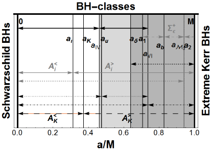
Figure 13: Representations of the main classes of attractors defined in accordance with the dimensionaless spins. It follows the analysis of the Sec. III. See also Figs 6.

Table 6: Definition of angular momenta $(\ell^{\pm}_{\varrho},\ell_{\mu}^{-})$. See also Table 2, Figs 6 and Table 4.

${\ell}_{*}:V_{eff}({\ell}_{*},r_{\mathrm{mso}}^{+})=1$	$\ell^{\pm}_{\varrho}(a/M):\;V_{eff}(\ell^{\pm}_{\varrho},r_{\mathrm{mso}}^{\pm})=1$
${\ell}_{\beta}^{-}:\;V_{eff}(\ell_{\beta}^{-},r_{\mathrm{mbo}}^{+})<1$	$\ell_{\Gamma}^{-}:\;V_{eff}(\ell_{\Gamma}^{-},r_{\gamma}^{+})=1$
$\ell_{\mu}^{-}:\;V_{eff}(\ell_{2}^{+},r_{\mathrm{mso}}^{-})=1$	$\ell_{q}^{-}\equiv{\ell_{\varrho}}^{-}\in\mathbf{L2}$

References

- Abbassi et al. (2013) Abbassi, S., Nourbakhsh, E., & Shadmehri, M. 2013, Astrophys. J. , 765, 96
- Abramowicz (1971) Abramowicz, M. A. 1971, Acta. Astron., 21, 81
- Abramowicz (2008) Abramowicz, M. A. 2008, arXiv:astro-ph/0812.3924
- Abramowicz et al. (1983) Abramowicz, M. A., Calvani, M. & Nobili, L. 1983, Nature (London), 302, 597–599
- Abramowicz & Fragile (2013) Abramowicz, M. A. & Fragile, P.C. 2013, Living Rev. Relativity, 16, 1
- Abramowicz et al. (2010) Abramowicz, M.A., Jaroszynski, M., Kato, S., et al. 2010, A & A, 521, A15
- Abramowicz et al. (1998) Abramowicz, M. A., Karas, V. & Lanza, A. 1998, A&A, 331, 1143
- Adamek & Stuchlik (2013) Adamek K. and Stuchlik Z. 2013, Class. Quant. Grav., 30, 205007
- Agol & Krolik (2000) Agol, E. & Krolik, J. 2000, Astrophys. J. , 528, 161
- Alexander et al. (2008) Alexander, R. D., Armitage, P. J., Cuadra, J., et al.2008, Astrophys. J. , 674, 927 ,
- Alig et al. (2013) Alig, C., Schartmann, M., Burkert, et al.2013, Astrophys. J. , 771, 2, 119
- Allen et al. (2006) Allen, S. W., Dunn, R.J.H., Fabian, A.C., et al. 2006, MNRAS, 1, 372, 21
- Almeida & Ricci (2017) Almeida C. R. & Ricci C. 2017, Nature (London)Astron. 1, 679-689
- Aly et al. (2015) Aly, H., Dehnen, W., Nixon, C.et al. 2015, MNRAS, 449, 1, 65
- Andrade-Santos et al. (2016) Andrade-Santos, F., Bogdán, Á., Romani, R. W., et al. 2016, Astrophys. J. , 826, 91
- Anthony & Carlberg (1988) Anthony, D. M., & Carlberg, R. G. 1988, Astrophys. J. , 332, 637
- Armitage & Natarajan (1999) Armitage, P. J., & Natarajan, P. 1999, Astrophys. J. , 525, 909
- Balbus & Hawley (1991) Balbus, S. A., & Hawley, J. F. 1991, Astrophys. J. , 376, 214
- Banados et al. (2017) Banados, E. et al. 2018, Nature, 553, 7689 473
- Bao & Stuchlík (1992) Bao, G., & Stuchlík, Z. 1992, Astrophys. J. , 400, 163
- Bardeen et al. (1973) Bardeen, J. M., Carter, B., & Hawking, S. W. 1973, Communications in Mathematical Physics, 31, 161
- Bardeen & Petterson (1975) Bardeen, J.M., Petterson, J.A., 1975, Astrophys. J. , 195, L65
- Bertin & Lodato (1999) Bertin, G., & Lodato, G. 1999, A&A, 350, 694
- Bertin & Lodato (2001) Bertin, G., & Lodato, G. 2001, A & A, 370, 342
- Blaschke & Stuchlík (2016) Blaschke, M. & Stuchlík, Z. 2016, Phys. Rev. D, 94, 8, 086006
- Bogdán et al. (2018) Bogdán, Á., Lovisari, L., Volonteri, M., & Dubois, Y. 2018, Astrophys. J. , 852, 131
- Bogdan et al. (2017) Bogdsn, A., Kraft, R. P., Evans, D. A., et al. 2017, Astrophys. J. 848, 1, 61
- Bonnell & Rice (2008) Bonnell, I. A., & Rice, W. K. M. 2008, Science, 321, 1060
- Bonnerot et al. (2016) Bonnerot, C., Rossi, E. M., Lodato, G.et al. 2016, MNRAS, 455, 2, 2253
- Boyer (1965) Boyer, R.H. 1965, Proc. Camb. Phil. Soc., 61, 527
- Bromley et al. (1998) Bromley, B. C., Miller, W. A. & Pariev, V. I. 1998, Nature (London), 391, 54, 756
- Bugli et al. (2017) Bugli, M., Guilet, J., Muller, E., et al. 2017, arXiv:1707.01860
- Capellupo et al. (2017) Capellupo, D. M., Wafflard-Fernandez, G. & Haggard, D. 2017, Astrophys. J. , 836, 1, L8
- Caproni et al. (2017) Caproni, A., Abraham, Z., Motter, J. C. et al. 2017, Astrophys. J. , 851, 2, L39
- Carmona-Loaiza et al. (2015) Carmona-Loaiza, J.M., Colpi, M., Dotti, M., et al. 2015, MNRAS, 453, 1608
- Carpano & Jin (2018) Carpano, S., & Jin, C. 2018, MNRAS, 477, 3178
- Chen et al. (2015) Chen, Y., Zhang, X., Zhang, H., et al. 2015, apss, 357, 2, 100
- Daly (2009) Daly, R. A. 2009, Astrophys. J. , 691, L72
- D’Ammando (2017) D’Ammando F. 2017, Front. Astron. Space Sci. 4, 53
- Das et al. (2017) Das, U., Begelman, M. C. & Lesur, G., 2017, MNRAS, 473, 2791
- DeGraf et al. (2017) DeGraf, C., Dekel, A., Gabor, J. et al. 2017, MNRAS, 466, 1462
- Del Zanna et al. (2007) Del Zanna, L., Zanotti, O., Bucciantini, N., et al. 2007, A & A, 473, 11
- Doeleman et al. (2008) Doeleman, S. et al. 2008, Nature, 455, 78
- Doğan et al. (2015) Doğan, S., Nixon, C., King, A.et al. 2015, MNRAS, 449, 1251
- Duran et al. (2017) Duran, R. B., Tchekhovskoy, A. and Giannios, D. 2017, MNRAS, 469, 4, 4957
- Dyda et al. (2015) Dyda, S., Lovelace, R.V.E., Ustyugova, et al.2015, MNRAS, 446, 613
- Fang & Murase (2018) Fang, K. & Murase, K. 2018, Nature Physics, Letter doi:10.1038/s41567-017-0025-4
- Farr et al. (2017) Farr, W. M., Stevenson, S., Coleman Miller, M., et al. 2017, Nature (London), 548, 426
- Fender (2001) Fender, R. P. 2001, MNRAS, 322, 31–42
- Fender (2009) Fender, R. P. 2010, Lect. Notes Phys. 794, 115
- Fender & Belloni (2004) Fender, R. & Belloni, T. 2004, Ann. Rev. Astron. Astrophys. 42, 317
- Fender et al. (1998) Fender, R. P., Garrington, S. T., McKay, D. J., et al. 1998, New Astronomy Reviews, 42, 593
- Fender et al. (1999) Fender, R. P., Garrington, S. T., McKay, D. J., et al. 1999, MNRAS, 304, 865
- Fender & Pooley (1998) Fender, R. P., & Pooley, G. G. 1998, MNRAS, 300, 573
- Fernández-López et al. (2017) Fernández-López, M., Zapata, L. A., & Gabbasov, R. 2017, Astrophys. J. , 845, 10
- Font & Daigne (2002a) Font, J. A. & Daigne, F. 2002a, MNRAS, 334, 383
- Font & Daigne (2002b) Font, J. A. & Daigne, F. 2002b, Astrophys. J. , 581, L23–L26
- Fuerst & Wu (2007) Fuerst, S. V. & Wu, K., 2007, A&A 474, 55-7
- Gandhi et al. (2017) Gandhi, P. et al. 2017, arXiv:1710.09838
- Gelli et al. (2007) Gilli, R., Comastri, A. and Hasinger, G. 2007, A&A, 463, 79
- Ghasemnezhad & Abbassi (2016) Ghasemnezhad, M. & Abbassi, S. 2016, MNRAS, 456, 1, 71
- Ghisellini et al. (2014) Ghisellini, G., Tavecchio, F., Maraschi, L., et al. 2014 Nature (London), 515, 376
- Hamersky & Karas (2013) Hamersky, J. & Karas, V. 2013, A&A, 32, 555
- Harrison (2013) Harrison, F. A.et al. 2013, Astrophys. J. , 770, 103
- Herrnstein et al. (1998a) Herrnstein, J. R., Moran, J. M., Greenhill, L. J., et al. 1998, Astrophys. J. , 508, 243
- Herrnstein et al. (1998b) Herrnstein, J. R., Greenhill, L. J., Moran, J. M., et al. 1998, Astrophys. J. L, 497, L69
- Hirano et al. (2017) Hirano, S., Hosokawa T., Yoshida, N., Kuiper, R. 2017, Science, 29, 357, 6358, 1375-1378
- Humphreys et al. (2008) Humphreys, E. M. L., Reid, M. J., Greenhill, L. J., et al.2008, Astrophys. J. , 672, 800
- Hunter (1963) Hunter, C. 1963, MNRAS, 126, 299
- Igumenshchev (2000) Igumenshchev, I. V. & Abramowicz, M. A. 2000, APJS, 130, 463
- Ingram et al. (2016) Ingram, A., van der Klis, M., Middleton, M. et al. 2016,MNRAS, 461, 2, 1967
- Inoue et al. (2017) Inoue, Y., Doi, A., Tanaka, Y. T., et al. 2017, Astrophys. J. 840, 1, 46
- Karas & Sochora (2010) Karas, V. & Sochora, V., 2010, Astrophys. J. , 725, 2, 1507–1515
- Kawakatu & Ohsuga (2011) Kawakatu, N., Ohsuga, K. 2011, MNRAS, 417, 4, 2562-2570
- King et al. (2005) King, A. R., Lubow, S. H., Ogilvie, et al. 2005, MNRAS, 363, 49
- Kiuchi et al. (2011) Kiuchi, K., Shibata, K., Montero, P. J. & Fontv J. A., 2011, Phys. Rev. Lett. , 106, 251102
- Komossa (2015) Komossa, S. 2015, JHEAp, 7,148
- Kondratko et al. (2008) Kondratko, P. T., Greenhill, L. J. and Moran, J. M. 2008, Astrophys. J. , 678, 87
- Korobkin et al. (2013) Korobkin, O., Abdikamalov, E., Stergioulas, N., et al. 2013, MNRAS, 431, 1, 354
- Kubsch et al. (2016) Kubsch, M., Illenseer, T. F., & Duschl, W. J. 2016, A&A, 588, A22
- Krolik & Hawley (2002) Krolik, J.H. & Hawley, J.F. 2002, Astrophys. J. , 573, 754
- Kozlowski et al. (1978) Kozlowski, M., Jaroszynski, M. & Abramowicz, M. A. 1978, A & A 63, 1–2, 209–220.
- Lasota et. al. (2016) Lasota, J.-P., Vieira, R.S.S., Sadowski,et al. 2016, A & A., 587, A13
- Lee et al. (2017a) Lee, C., Li, Z., Ho, P. et al. 2017,Science Advs. 3, e1602935
- Lee et al. (2017b) Lee, C., Ho, P., Li, Z. Li, et al. 2017 Nature (London)Astron., 1, 0152
- Lei et al. (2008) Lei, Q., Abramowicz, M. A., Fragile, et al.2008, A&A., 498, 471
- Li (2012) Li., L. X. 2012, MNRAS, 424, 1461
- Liska et al. (2018) Liska, M., Hesp, H., Tchekhovskoy, A., et al. 2018, MNRAS: Letters, 474
- Lodato & Pringle (2006) Lodato, G., & Pringle, J. E. 2006, MNRAS, 368, 1196
- Lodato (2007) Lodato, G. 2007, Riv. Nuovo Cim., 2007, 30, 293
- Lovelace & Chou (1996) Lovelace, R. V. E. & Chou, T. 1996, Astrophys. J. , 468, L25
- Lovelace et al. (2014) Lovelace, R. V.E., Romanova, M. M., Lii, P.et al. 2014, Comp. Astroph. Cosmology 1-3
- Lynden-Bell & Pringle (1974) Lynden-Bell, D., & Pringle, J. E. 1974, MNRAS, 168, 603
- Lyutikov (2009) Lyutikov, M. 2009, MNRAS, 396, 3, 1545–1552
- Madau (1988) Madau, P. 1988, Astrophys. J. , 1, 327, 116-127
- Maitra et al. (2009) Maitra, D., Markoff, S., Brocksopp C., et al. 2009, MNRAS, 398, 4, 1638–1650
- Maraschi & Tavecchio (2003) Maraschi, L. & Tavecchio, F. 2003, Astrophys. J. , 593, 667
- Marchesi et al. (2016) Marchesi, S. et al. 2016, Astrophys. J. , 830, 100, 20
- Marchesi et al. (2017) Marchesi, S., Ajello, M., Comastri A., et al. 2017, Astrophys. J. , 836, 1, 116
- Marscher et al. (2002) Marscher, A. P., Jorstad, S. G., Gomez, J. L., et al. 2002, Nature (London), 417, 625–627
- Martin et al. (2009) Martin, R. G., Pringle, J. E., & Tout, C. A. 2009, MNRAS, 400, 383
- Masini et al. (2016) Masini, A. et al. 2016, A&A, 589, A59
- May (1976) May, R. M. 1976, Nature 261, 459–467
- McClintock et al. (2006) McClintock, J. E., Shafee, R., Narayan, R., et al. 2006,Astrophys. J. , 652, 518
- Mewes et al. (2016) Mewes, V., Font, J. A., Galeazzi, F. et al. 2016. Phys. Rev. D, 93, 6, 064055
- Montero et al. (2007) Montero, P. J., Zanotti, O., Font, J. A. & Rezzolla, L., 2007, MNRAS, 378, 1101
- Moran (2008) Moran, J. M., ASP Conf. Ser. 395 (2008) 87
- Morningstar et al. (2014) Morningstar, W. R., Miller, J. M., Reis, R. C. et al.2014, Astrophys. J. , 784, L18
- Mossoux et al. (2014) Mossoux, E., Grosso, N., Vincent, F. H. et al.2015, A&A, 573, A46
- Narayan & McClintock (2013) Narayan R. & McClintock, J. E. 2013, arXiv:1312.6698
- Neilsen & Lee (2009) Neilsen, J. & Lee, J. C. 2009, Nature 458, 481, 1–74
- Nelson & Papaloizou (2000) Nelson, R. P. & Papaloizou, J. C. B., 2000, MNRAS, 315, 570
- Nixon et al. (2013) Nixon, C., King, A. & Price, D. 2013, MNRAS, 434, 1946
- Oka et al. (2017) Oka, T., Tsujimoto, S., Iwata, Y., 2017, Nature Astronomy-Letter, doi:10.1038/s41550-017-0224
- Okuda & Das (2015) Okuda, T. & Das, S. 2015, MNRAS, 453, 1, 147
- Paczyński (1980) Paczyński, B. 1980, Acta Astron., 30, 4
- Paczyński (2000) Paczyński, B. 2000, astro-ph/0004129.
- Perego et al. (2009) Perego, A., Dotti, M., Colpi, M., & Volonteri, M. 2009, MNRAS, 399, 2249
- Porth et al. (2017) Porth, O.et al. 2017, CompA, 4, 1
- Pugliese & Kroon (2012) Pugliese, D. & Kroon, J. A. V. 2012, Gen. Rel. Grav., 44, 2785
- Pugliese & Montani (2013) Pugliese, D. & Montani, G. 2013, EPL, 101, 1, 19001
- Pugliese & Montani (2015) Pugliese, D. & Montani, G. 2015, Phys. Rev. D, 91, 083011
- Pugliese & Montani (2018) Pugliese, D. & Montani, G. 2018, MNRAS, 476, 4346
- Pugliese et al (2012) Pugliese, D., Montani, G. & Bernardini, M. G. 2012, MNRAS, 428, 2, 952
- Pugliese & Quevedo (2015) Pugliese, D. & Quevedo, H. 2015, Eur. Phys. J. C, 75, 5, 234
- Pugliese et al. (2011a) Pugliese, D., Quevedo, H., & Ruffini, R. 2011a, Phys. Rev. D, 83, 024021
- Pugliese et al. (2011b) Pugliese, D., Quevedo, H. & Ruffini, R. 2011, Phys. Rev. D, 84, 044030
- Pugliese et al. (2013) Pugliese, D., Quevedo, H. & Ruffini, R. 2013, Phys. Rev. D, 88, 2, 024042
- Pugliese & Stuchlík (2015) Pugliese, D. & Stuchlík, Z. 2015, APJS, 221, 2, 25
- Pugliese & Stuchlík (2016) Pugliese, D. & Stuchlík, Z. 2016, APJS, 223, 2, 27
- Pugliese & Stuchlík (2017) Pugliese, D. & Stuchlík, Z. 2017, APJS, 229, 2, 40
- Pugliese & Stuchlík (2018a) Pugliese, D. & Stuchlík, Z. 2018, Class. Quant. Grav., 35, 105005
- Pugliese & Stuchlík (2018a) Pugliese, D. & Stuchlík, Z. 2018a, JHEAp 17, 1
- Pürrer et al. (2016) Pürrer, M., Hannam, M., & Ohme, F. 2016, Phys. Rev. D, 93, 084042
- Qin et al. (2008) Qin, S. L., Zhao, J. H. et al. 2008, Astrophys. J. , 677, 353
- Regan et al. (2017) Regan, J., Visbal, E., Wise, J. H., et al. 2017 arXiv:1703.03805
- Rezzolla et al. (2003) Rezzolla, L., Zanotti, O. & Font, J. A. 2003, A & A, 412, 603
- Ricci et al. (2017a) Ricci, C. et al. 2017, Nature (London), 549, 488
- Ricci et al. (2017b) Ricci, C. et al. 2017, MNRAS, 468, 1273
- Rodriguez et al. (2008) Rodriguez, L. F., Moran, J. M., Franco-Hernandez, R., et al. 2008, Astron. J. 135, 2370
- Sadowski et al. (2016) Sadowski, A., Lasota, J.P., Abramowicz, M.A. & Narayan, R. 2016, MNRAS, 456, 4, 3915-3928
- Sbarrato et al. (2014) Sbarrato, T., Padovani, P. & Ghisellini, G. 2014, MNRAS, 445, 1, 81.
- Schee & Stuchlík (2009) Schee, J. & Stuchlík, Z. 2009, Gen. Rel. Grav., 41, 1795
- Schee & Stuchlík (2013) Schee, J. & Stuchlík, Z. 2013, JCAP, 2013
- Scheuer & Feiler (1996) Scheuer, P. A. G., & Feiler, R. 1996, MNRAS, 282, 291
- Slany & Stuchlík (2005) Slany, P. & Stuchlík, Z. 2005, Class. Quant. Grav., 22, 17
- Shadmehri & Khajenab (2006) Shadmehri, M. & Khajenab, F. 2006, Astrophys. J. , 637, 1
- Shlosman & Begelman (1987) Shlosman, I. & Begelman, M. C., 1987, Nature 329, 810-812
- Shlosman & Begelman (1989) Shlosman, I., & Begelman, M. C. 1989, Astrophys. J. , 341, 685
- Sikora (1981) Sikora, M. 1981, MNRAS, 196, 257
- Sochora et al. (2011) Sochora, V., Karas, V., Svoboda, J. & Dovciak, M. 2011, MNRAS, 418, 276–283
- Soleri et al. (2010) Soleri, P. et al. 2010, MNRAS, 406, 1471
- Stalevski et al. (2012) Stalevski, M., Fritz, J. et al. 2012, MNRAS, 420, 2756-2772
- Stollman & van Paradijs (1985) Stollman, G. M., & van Paradijs, J. 1985, A&A, 153, 99
- Stone et al. (2018) Stone, N. C., Kesden, M., Cheng, R. M., & van Velzen, S. 2018, arXiv:1801.10180
- Storchi-Bergmann et al. (2017) Storchi-Bergmann, T., Schimoia, J. S., Peterson, B. M., et al. 2017, Astrophys. J. , 835, 2
- Stuchlík (1980) Stuchlík, Z. 1980, Bull. astr. Inst. Czechosl. vol. 31, 3, 1980, 12–144
- Stuchlík (1981a) Stuchlík, Z. 1981a, Bull. astr. Inst. Czechosl., 32, 1, 40
- Stuchlík (1981b) Stuchlík, Z. 1981b, Bull. astr. Inst. Czechosl., 32, 6, 366-373
- Stuchlík (1983) Stuchlík, Z., 1983, Bull. astr. Inst. Czechosl., 34, 3, 129-149
- Stuchlík (2005) Stuchlík, Z. 2005, Mod. Phys. Lett. A, 20, 561
- Stuchlík & Hledik (1999) Stuchlík, Z. & Hledik, S. 1999, Phys. Rev. D60, 044006
- Stuchlík & Kotrlova (2008) Stuchlík, Z. & Kotrlova, A., 2009, Gen. Rel. Grav., 41, 1305
- Stuchlík et al. (2013) Stuchlík, Z., Kotrlová, A., & Török, G. 2013, A&A, 552, A10
- Stuchlík & Kovar (2008) Stuchlík, Z. & Kovar, J. 2008, Int. J. Mod. Phys. D, 17, 2089
- Stuchlík & Schee (2010) Stuchlík, Z. & Schee, J. 2010, Class. Quant. Grav., 27, 215017
- Stuchlík & Schee (2012) Stuchlík, Z. & Schee, J. 2012, Class. Quant. Grav., 29, 065002
- Stuchlík & Slany (2004) Stuchlík, Z. & Slany, P. 2004, Phys. Rev. D, 69, 064001.
- Stuchlík et al. (2000) Stuchlík, Z., Slany, P. & Hledik, S 2000, A & A 363, 425-439
- Stuchlík et al. (2009) Stuchlík, Z., Slany, P., & Kovar, J. 2009, Class. Quant. Grav., 26, 215013
- Stuchlík et al. (2005) Stuchlík, Z., Slany, P. Torok, & Abramowicz, M. A. 2005, Phys. Rev. D, 71, 024037
- Tetarenko et al. (2018) Tetarenko, B. E., Lasota, J.-P., Heinke, C. O., et al. 2018, Nature, 554, 69–72
- Toba et al. (2017) Toba, Y., Komugi, S., Nagao, T., et al. 2017, Astrophys. J. , 851, 98
- Tohline & Hachisu (1990) Tohline, J. E., & Hachisu, I. 1990, Astrophys. J. , 361, 394
- van Paradijs & Stollman (1984) van Paradijs, J., & Stollman, G. M. 1984, A&A, 137, L12
- van Putten (2012) van Putten, M. H. P. M. 2012, Prog. Theor. Phys., 127, 331
- van Putten (2015) van Putten, M. H. P. M. 2015, Astrophys. J. , 810, 1, 7
- van Putten & Della Valle (2017) van Putten, M. H. P. M. & Della Valle, M. 2017, MNRAS, 464, 3, 3219
- Vedantham et al. (2017) Vedantham, H. K. et al. 2017, Astrophys. J. 845 2, 89
- Volonteri (2007) Volonteri, M., 2007, ApJ, 663, L5
- Volonteri (2010) Volonteri, M., 2010, A & AR, 18, 279
- Volonteri et al. (2003a) Volonteri, M., Haardt, F. & Madau, P. 2003, Astrophys. J. , 582 559
- Volonteri et al. (2007) Volonteri, M., Sikora, M., Lasota, J.-P., 2007, ApJ, 667, 704
- von Weizsäcker (1951) von Weizsäcker, C. F. 1951, Astrophys. J. , 114, 165
- Weber & Davis (1967) Weber, E. J., & Davis, L., Jr. 1967, Astrophys. J. , 148, 217
- Wielgus et al. (2015) Wielgus, M., Fragile, P. C., Wang, Z., & Wilson, J. 2015, MNRAS, 447, 359
- Woodward et al. (1994) Woodward, J. W., Tohline, J. E., & Hachisu, I. 1994, Astrophys. J. , 420, 247
- Yang et al. (2017) Yang, G. et al. 2017, arXiv:1710.09399
- Yu et al. (2015) Yu, X., Zhang, X., Zhang, H., Xiong, D., et a. 2015, Ap&SS, 357, 14
- Xie & Yuan (2017) Xie, F. G. & Yuan, F. 2017, Astrophys. J. , 836, 1, 104
- Zanotti & Pugliese (2015) Zanotti, O. & Pugliese, D. 2015, Gen. Rel. Grav., 47, 4, 44
- Zhang et al. (2015) Zhang, J., Xue, Z.W., He, J.J., et al. 2015, Astrophys. J. , 807, 1, 51