Discovery of two embedded massive YSOs and an outflow in IRAS 18144-1723

Abstract

Massive stars are rarely seen to form in isolation. It has been proposed that association with companions or clusters in the formative stages is vital to their mass accumulation. In this paper we study IRAS 18144-1723, a massive young stellar object (YSO) which had been perceived in early studies as a single source. In the CO(3-2) line, we detect an outflow aligned well with the outflow seen in H₂ in this region. We show that there are at least two YSOs here, and that the outflow is most likely to be from a deeply embedded source detected in our infrared imaging. Using multi-wavelength observations, we study the outflow and the embedded source and derive their properties. We conclude that IRAS 18144 hosts an isolated cloud, in which at least two massive YSOs are being born. From our sub-mm observations, we derive the mass of the cloud and the core hosting the YSOs.

1 Introduction

Recent studies suggest that the primary mechanism for the formation of massive stars is disk accretion as in their low-mass counterparts (Arce et al., 2007; Beuther et al., 2002a; Varricatt et al., 2010; Davis et al., 2004). Collimated outflows discovered from massive star forming regions in these studies indicate the presence of accretion discs. The cavities carved by the protostellars outflow provide a path for the radiation to escape, thereby reducing the radiation pressure on the accreted matter and allowing the mass accumulation in massive YSOs through accretion (Krumholz, McKee & Klein, 2005). However, unlike low-mass stars, massive stars are rarely observed to form in isolation. Instead, they are seen to be associated with companions or clusters suggesting that such associations may play a prominent role in their formation (Lada & Lada, 2003). Massive YSOs are located in the galactic plane at large distances from us, so we need observations at infrared and longer wavelengths at high angular resolution to understand their formation. With the availability of large telescopes operating at these wavelengths, many of the massive YSOs, which appeared to form in isolation in older studies, are now being resolved into binaries or multiples (e.g. Varricatt et al. (2010)). In this paper, we present a detailed observational study of the massive YSO IRAS 18144-1723 (hereafter IRAS 18144).

IRAS 18144 is located near the galactic plane (l=13.657^∘, b=-0.6^∘), and is associated with a dense core of far-IR luminosity 1.32$\times$10⁴ L_⊙, detected in NH₃ emission (Molinari et al., 1996). Using the line-of-sight radial velocity of the NH₃ emission (+47.3 km s^-1), they derived a kinematic distance of 4.33 kpc. Water and methanol masers are also detected from this source (Palla et al., 1991; Szymczak et al., 2000; Kurtz et al., 2004; Gómez-Ruiz et al., 2016). Molinari et al. (1998) did not detect 6-cm radio emission associated with the IRAS source sugessting that it is in a pre-UCHii stage. Observations by Zhang et al. (2005) did not detect any CO(2–1) outflow towards this region. However, through near-IR imaging in the H₂ line at 2.1218 $\mu$m and in the $K$ filter, Varricatt et al. (2010) discovered an E–W jet appearing to emanate from a bright near-infrared source (referred to as ‘A’) located at $\alpha$=18:17:24.38, $\delta$=-17:22:14.7. We further observed this region at multiple wavelengths from near-IR to sub-mm in order to uncover the nature and possible multiplicity of source ‘A’. The new observations are analysed along with archival data.

2 Observations and data reduction

2.1 Near-IR imaging with WFCAM

We observed IRAS 18144 using the United Kingdom Infrared Telescope (UKIRT), Hawaii, and the UKIRT Wide Field Camera (WFCAM; Casali et al. (2007)). WFCAM employs four 2048$\times$2048 HgCdTe HawaiiII arrays, each with a field of view of 13.5′$\times$13.5′at an image scale of 0.4″ pixel^-1.

Observations were obtained in the the near-IR $J,H$ and $K$-band filters, and in narrowband filters centred on the H₂ $\upsilon$ = 1–0 S(1) line at 2.1218 $\mu$m and the [Fe II] $a^{4}D_{7/2}-a^{4}F_{9/2}$ forbidden emission line at 1.6439 $\mu$m. H₂ and [Fe ii] are good tracers of star formation activity. H₂ emission may be fluorescently excited in photodissociation regions associated with massive and intermediate mass young stars or in planetary nebulae, or shock excited in jets and warm entrained molecular outflows from YSOs. [Fe II] is often used as a tracer of ionized region at the base of the jet (Davis et al., 2011).

Table 1: Imaging observations using WFCAM and UIST

UTDate	Filters	Exp. time	Int. time	FWHM
yyyymmdd		(sec)	(sec)	(arcsec)
WFCAM
20140620	$J$	10,2	360, 40	1.11, 1.10
20140620	$H$	5,1	180, 20	1.10, 1.21
20140620	$K$	5,1	180, 20	1.05, 0.91
20140620	1-0S1	40	1440	1.07
20140621	1-0S1	40	2$\times$1440	0.82, 0.79
20140621	$J$	10	360	0.84
20140621	$H,K$	5,5	180, 180	0.78, 0.77
20140622	1.644FeII	40	1440	0.79
20140623	1.644FeII	40	1440	0.86
20170522	$J$	5	720	0.99
20170522	$H,K$	5, 5	360, 180	0.82, 0.84
20180330	$J$	5	720	0.94
20180330	$H,K$	5, 5	360, 180	0.88, 0.87
UIST
20140820	$L^{\prime}$	0.4$\times$50a	160	0.48
20140820	$M^{\prime}$	0.175$\times$50	105	0.5

• ^aexp. time $\times$ coadds

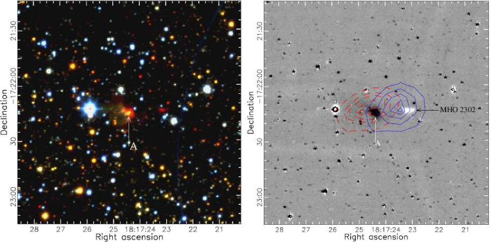
Figure 1: Left: A $2\arcmin\times 2\arcmin$ field of the $J$ (blue), $H$ (green), $H_{2}$ (red) colour composite image of IRAS 18144 observed using WFCAM. Right: The continuum-subtracted H₂ image of the same field. The blue (continuous) and red (dashed) contours are generated from the CO(3–2) intensity maps of the blue- and red-shifted lobes of the outflow detected in our JCMT+HARP observations, integrated in velocity ranges of 23.3 – 44.0 km s^-1 and 50.6 – 71.3 km s^-1 respectively. The H₂ emission knot MHO 2302 and the outflow source candidate (‘A’) identified by Varricatt et al. (2010) are labelled.

The observations were performed by dithering the object to nine positions separated by a few arcseconds and using a 2$\times$2 microstep, resulting in a pixel scale of 0.2″ pixel^-1. The sky conditions were clear. Table 1 gives a log of the WFCAM observations. Preliminary reduction of the data was performed by the Cambridge Astronomical Survey Unit (CASU). The photometric system and calibration are described in Hewett et al. (2006) and Hodgkin et al. (2009) respectively. The pipeline processing and science archive are described in Irwin et al. (2004) and Hambly et al. (2008). Further reduction was carried out using the Starlink packages kappa and ccdpack. The left panel of Fig. 1 shows a J,H,H₂ ($J$-blue, $H$-green, $H_{2}$-red) colour composite image in a 2$\arcmin\times$2$\arcmin$ field centred on IRAS 18144. The long-integration $J$ and $H$ images obtained on UT 20140620 and 20140621 and both $H_{2}$ images obtained on 20140620 were averaged for constructing Fig. 1. The narrow-band H₂ and [Fe ii] images were continuum subtracted using scaled K and H images respectively observed closest in time as well as with good agreement in seeing, adopting the procedure given in Varricatt et al. (2010). The right panel of Fig. 1 shows the continuum-subtracted H₂ image. The extended emission features are continuum subtracted well. The point sources show positive or negative residuals due to the difference in seeing between the two images or due to reddening. The H₂ emission knot (MHO 2302) and the outflow source candidate (‘A’) identified by Varricatt et al. (2010) are labelled. No line emission was detected in the [Fe ii] image, so it is not shown here.

Source ‘A’ of Varricatt et al. (2010) is detected well in our $K$-band image as a highly reddened object embedded in nebulosity (see §3.2). Its detection is marginal in $H$, and most of the emission is from the nebulosity. It is not detected in $J$; only the nebulosity is seen.

2.2 $L^{\prime}$ and $M^{\prime}$ imaging using UIST

$L^{\prime}$ (3.77 $\mu$m) and $M^{\prime}$ (4.69 $\mu$m) imaging observations were obtained using the UKIRT 1–5 $\mu$m Imager Spectrometer (UIST, Ramsay Howat et al. (2004)). UIST employs a 1024$\times$1024 InSb array. The 0.12″ pixel^-1 camera of UIST was used, which has an imaging field of 2′$\times$2′ per frame. The observations were performed by dithering the object to four positions on the array, separated by 20″ each in RA and Dec from the base position. Each pair of observations was flat-fielded and mutually subtracted, resulting in a positive and negative beam. The final mosaic was constructed by combining the positive and negative beams. Table 1 gives the details of the observations.

The data reduction was carried out using the facility pipeline oracdr (Cavanagh et al., 2008) and using kappa and ccdpack. Astrometric calibration was done using the 2MASS positions of the objects detected in our images. The UKIRT standard star GL748 was observed with the same dither pattern for photometric calibration. Fig. 2 shows a 25″$\times 25\arcsec$ section of the $M^{\prime}$ image. Source ‘A’ was detected well in $L^{\prime}$ band as a single object. In $M^{\prime}$, we detect a deeply embedded source $\sim$2.6″ NE of ‘A’; it is labelled ‘B’ on the figure. The magnitudes for sources ‘A’ and ‘B’ derived from our images are given in Table 2.

Table 2: Results from UIST imaging

Src	RA	Dec	magnitudesb
ID			$L^{\prime}$	$M^{\prime}$
A	18:17:24.375	-17:22:14.71	6.54 (0.04)	5.57 (0.07)
B	18:17:24.239a	-17:22:12.87a	Not det.	9.57 (0.14)

• ^aDerived from the Michelle image after matching the coordinates of source ‘A’ derived from the $K$-band image; ^bA 4″-diameter photometric aperture was used. ‘B’ being faint, a 1.2″-diameter aperture was used and aperture correction was applied. The values given in parenthesis are the 1-$\sigma$ errors in photometry.

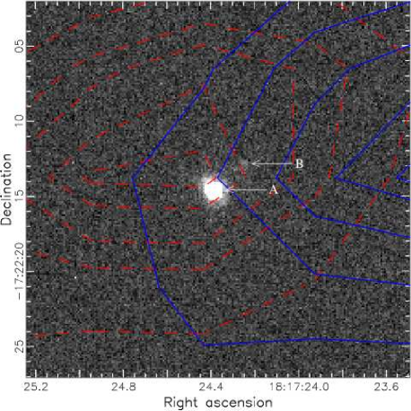
Figure 2: A $25\arcsec\times 25\arcsec$ field of the $M^{\prime}$ image of IRAS 18144 observed using UKIRT and UIST. The blue (continuous) and red (dashed) contours are generated from the integrated CO(3–2) maps of the red- and blue-shifted lobes of the outflow.

2.3 Michelle imaging

Michelle (Glasse, Atad-Ettedgui & Harris, 1997) is a mid-IR imager/spectrometer at UKIRT, employing an SBRC Si:As 320$\times$240-pixel array. It has a field of view of 67.2″$\times$50.4″with an image scale of 0.21″ pix^-1. We observed IRAS 18144 using Michelle on multiple nights in four filters centered at 7.9, 11.6, 12.5 and 18.5 $\mu$m. The 7.9 $\mu$m filter has a 10% passband, and the other filters have 9% passbands.

The sky conditions were photometric with the atmospheric opacity at 225 GHz measured with the CSO (Caltech Submillimeter Observatory) dipper ($\tau_{225GHz}$) was $\sim$0.07. BS 6705 and BS 7525 were used as the standard stars on 20040329 UT, and BS 6869 was the standard for the rest of the observations. Table 3 shows the details of the observations. The details of the data reduction are the same as in Varricatt et al. (2013). Astrometric corrections were applied by adopting the position of source ‘A’ from Varricatt et al. (2010). Fig. 3 shows a colour composite image in a 25″$\times$25″ region constructed from our Michelle images at 18.5, 12.5 and 7.9 $\mu$m. Aperture photometry was performed using an aperture of diameter 14 pixels (2.94$\arcsec$). The flux densities measured for sources ‘A’ and ‘B’ are given in Table 3.

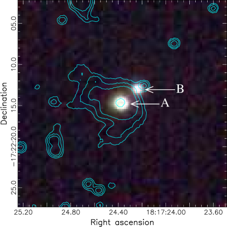
Figure 3: A colour composite image (18.5 $\mu$m (red), 12.5 $\mu$m (green), 7.9 $\mu$m (blue)) of a $25\arcsec\times 25\arcsec$ field from our Michelle images. The contours are generated from the $K$-band image presented in Varricatt et al. (2010), and are at arbitrary levels.

Table 3: Observations using UKIRT and Michelle

UTDate	Filter	Exp. time	Coadds	Int. time	FWHM	Flux density in Jya
		(sec)		(sec)	(arcsec)	Source ‘A’	Source ‘B’
20151107	7.9 $\mu$m	0.08	155	148.8	0.73	2.17 (0.16)	0.85 (0.1)
20160826	7.9 $\mu$m	0.08	155	248.0	0.72	2.02 (0.04)	0.92 (0.1)
20151107	11.6 $\mu$m	0.09	144	155.52	0.75	2.23 (0.04)	0.40 (0.05)
20160826	11.6 $\mu$m	0.09	144	259.2	0.76	1.93 (0.04)	0.40 (0.12)
20040329	12.5 $\mu$m	0.08	155	99.2	0.82	3.16 (0.18)	0.96 (0.13)
20160826	12.5 $\mu$m	0.07	168	141.12	0.83	2.55 (0.06)	0.93 (0.06)
20160920	12.5 $\mu$m	0.07	168	161.28	0.87	2.74 (0.13)	0.93 (0.07)
20151107	18.5 $\mu$m	0.03	338	162.24	1.08	5.27 (0.09)	2.41 (0.13)
20160826	18.5 $\mu$m	0.03	338	283.92	1.08	4.54 (0.04)	2.25 (0.06)
20160920	18.5 $\mu$m	0.03	338	162.24	1.02	5.63 (0.36)	2.28 (0.24)

• ^aThe values given in parenthesis are the 1-$\sigma$ errors in the flux density measured in the four beams from the Michelle image observed with chopping and nodding.

2.4 Archival imaging data

The field containing IRAS 18144 was covered in the Spitzer GLIMPSE survey using the Infrared Array Camera (IRAC; Fazio et al., 2004), and the MIPSGAL survey using MIPS (Rieke et al., 2004). We downloaded the IRAC images and catalogue and the MIPS images from the Spitzer Heritage Archive. Source ‘A’ was detected well in the IRAC bands 1–4 (centered at 3.5, 4.5, 5.8 and 8.0 $\mu$m respectively). ‘B’ was not detected in bands 1 and 2, and was only marginally detected in band 3. It was detected well in band 4, but the psf merges with that of ‘A’. The Spitzer catalog lists its location as ($\alpha$=18:17:24.25, $\delta$=-17:22:13.16), which agrees with our position (Table 2) within the 0.3″ error in the coordinates given in the GLIMPSE catalogue. IRAC 5.8 and 8.0 $\mu$m flux densities listed for this source are 264.0$\pm$30.2 and 534.4$\pm$56.5 mJy respectively. However, note that in UIST $M^{\prime}$ (4.7 $\mu$m), where ‘B’ is resolved well from ‘A’, source ‘B’ has a flux density of only 24.2$\pm$5 mJy (9.57 mag.; Table 2). The flux estimates of ‘B’ are likely to be affected by the proximity of ‘A’. Therefore, we do not use the 5.8 $\mu$m flux of ‘B’ in our analysis. The source is detected in the MIPS band 1 (23.68 $\mu$m) images at ($\alpha$=18:17:24.24, $\delta$=-17:22:12.61), but it is saturated making the photometry unusable. At a 2.45″ pix^-1 spatial resolution of the MIPS image, ‘A’ and ‘B’ are not resolved, but it should be noted that the centroid is much closer to ‘B’ than to ‘A’.

IRAS 18144 was observed in the WISE (Wright et al., 2010) and AKARI (Murakami et al., 2007) surveys. The sources ‘A’ and ‘B’ are not resolved by WISE. Our imaging at higher angular resolution shows that the emission from ‘A’ will the dominant source in the WISE bands W1, W2 and W3 at 3.4, 4.6, 12 $\mu$m respecitvely, so the magnitudes measured in those bands are not used in our analysis. Table 3 shows that ‘A’ contributes $\sim$70% of the total flux at 18.5 $\mu$m, so we use the band W4 (22 $\mu$m) magnitude of -1.191$\pm$0.011 as only an upper limit in the SED analysis. The flux densities measured in the AKARI-IRC 9 and 18 $\mu$m bands were not used in this study as they will be dominated by source ‘A’, and our Michelle observations at better spatial resolution cover these wavelengths. AKARI-FIS 90 and 140 $\mu$m flux densities were also not used as they will be affected by the large bandwidth of these filters. The FIS 65 and 160$\mu$m flux densities were used after applying the colour correction given in Yamamura et al. (2010).

We used the Herschel PACS (Poglitsch et al., 2010) (70 and 160 $\mu$m), and SPIRE (Griffin et al., 2010) (250 $\mu$m, 350 $\mu$m and 500 $\mu$m) level 2.5 maps (observation ID #1342218999 and #1342219000) publicly available from the Herschel Science Archive. ‘A’ and ‘B’ are not resolved in the Herschel maps. Aperture photometry of the source was performed using HIPE and aperture corrections were applied. Table 4 gives the flux densities for sources ‘A’ and ‘B’ combined, measured from the PACS and SPIRE maps.

Table 4: Flux density of ‘A+B’ from the Herschel maps

Wavelength	Aperture	Flux density	Error
($\mu$m)	diameter (arcsec)	(Jy)	(Jy)
70	24	525.6	20.5
160	44	938.6	27.7
250	44	454.5	18.8
350	60	191.7	12.4
500	84	74.7	2.2

2.5 Near-IR spectroscopy using UIST

We obtained near-IR spectroscopic observations of IRAS 18144 using UKIRT and UIST on UT 20140824. The sky conditions were clear with good seeing ($\sim$0.24″ in the $K$ band). The HK grism was used along with a 4-pix-wide (0.48″) slit, giving a wavelength coverage of 1.395–2.506 $\mu$m, and spectral resolution of $\sim$500. Flat field observations were obtained prior to the target observations by exposing the array to a black body mounted on the instrument. For wavelength calibration, the array was exposed to an Argon arc lamp. An early-type telluric standard was also observed at the same airmass as that of the target. We adopted a slit angle of 85.2^∘ West of North so that source ‘A’ and the H₂ emission feature MHO 2302 are both on the slit. For the target field, we nodded the telescope between the source position and a blank field nearby to enable good sky subtraction. The total on-chip exposure time for the target was 600 sec.

The data reduction was carried out using the UKIRT pipeline oracdr and Starlink kappa and figaro (Currie et al., 2008). The spectra from the two nodded beams of the reduced spectral image of standard star were extracted, averaged and wavelength calibrated. It was then divided by the spectrum of a blackbody of temperature similar to its photosperic temperature, and the photospheric absorption lines were interpolated out. The flat-fielded and sky-subtracted target spectal image was wavelength calibrated and divided by the interpolated standard star spectrum. The ratioed spectrum was then flux calibrated using the magnitudes of source ‘A’ derived from our photometry. Fig. 4 shows the calibrated spectral image of IRAS 18144. The extracted spectrum of source ‘A’ is shown in the upper panel of Fig. 5. The most prominent feature in the spectrum of source ‘A’ is the Br$\gamma$ emission line. The emission from MHO 2302 is composed purely of the ro-vibration lines of H₂. The spectrum of MHO 2302 extracted in 16 rows (7.68 arcsec²; the region shows in the dashed box in Fig. 4) is shown in the lower panel of Fig. 5. The integrated intensities of the H₂ lines measured from this spectrum are given in Table 5.

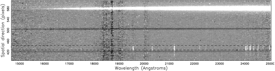
Figure 4: UIST spectral image of IRAS 18144 containing source ‘A’ and the outflow lobe MHO 2302. The image covers a wavelength regime of 14480–25059 Å on the X axis and has a spatial extent of 221 pixels (26.5$\arcsec$) on the Y axis. The dashed box show the region within which the spectrum of MHO 2302 is extracted

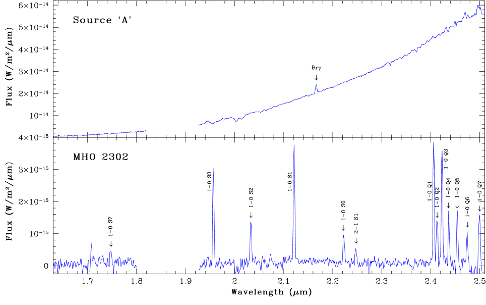
Figure 5: The upper panel shows the spectrum of source ‘A’. The lower panel shows the spectrum of MHO 2302, integrated over a field of 7.68 arcsec² (the region enclosed by the dashed box drawn in Fig. 4).

Table 5: H₂ line intensities

$\lambda_{air}$	Species	Intensity	Error	Einstein	ga	E($\upsilon$,J)
(Å)		W/m2	W/m2	A (s-1)		(K)
22235	1–0 S0	3.51E-18	4.00E-20	2.53E-7	5	6470
21218	1–0 S1	1.34E-17	2.00E-19	3.47E-7	21	6960
20338	1–0 S2	5.10E-18	5.00E-20	3.98E-7	9	7580
19576	1–0 S3	1.05E-17	2.00E-19	4.21E-7	33	8370
17480	1–0 S7	1.65E-18	1.50E-19	2.98E-7	57	12800
22477	2–1 S1	2.06E-18	4.00E-20	4.98E-7	21	12600
24066	1–0 Q1	1.27E-17	2.00E-19	4.29E-7	9	6150
24134	1–0 Q2	5.40E-18	2.00E-19	3.03E-7	5	6470
24237	1–0 Q3	1.24E-17	3.00E-19	2.78E-7	21	6960
24375	1–0 Q4	4.78E-18	1.00E-19	2.65E-7	9	7580
24548	1–0 Q5	6.43E-18	2.00E-19	2.55E-7	33	8370
24756	1–0 Q6	4.21E-18	1.50E-19	2.45E-7	13	9290
25001	1–0 Q7	8.88E-18	5.00E-19	2.34E-7	45	10300

• ^a Statistical weight

2.6 Sub-mm continuum observation using SCUBA-2

We observed IRAS 18144 using the James Clerk Maxwell Telescope (JCMT) and Submillimetre Common-User Bolometer Array 2 (SCUBA-2; Holland et al. (2013)) on UT 20140626. SCUBA-2 maps simulteneously at 450 and 850 $\mu$m. Each band uses four 32$\times$40 Transition Edge Sensor (TES) arrays, with a main beam size of 7.9″ and 13.0″ respectively at 450 $\mu$m and 850 $\mu$m.

The observation was performed by moving the telescope in a “CV Daisy” pseudo-circular pattern. A field of diameter of $\sim$12′ was obtained. The weather conditions were good with $\tau_{225\,GHz}$=0.08 during the observations. Pointing and extinction corrections were applied using pointing and flux standards observed before the target observations. The data reduction was performed using the Starlink package smurf. The maps were sampled down to 2″ pix^-1 at 450 $\mu$m and 4″ pix^-1 at 850 $\mu$m. We reach RMS noise levels of 2.04 mJy arcsec^-2 (213 mJy/beam) and 0.031 mJy arcsec^-2 (7 mJy/beam) respectively at the centers of the 450 $\mu$m and 850 $\mu$m maps.

Fig. 6 shows the central 4.5′$\times$4.5′ field extracted from the 850-$\mu$m SCUBA2 map. The SCUBA2 maps reveal a dense core associated with IRAS 18144. We measure an FWHM of 18.5″ and 22.6″ respectively at 450 $\mu$m and 850 $\mu$m. These are larger than the average FWHM of 9.35″ and 14.2″ respectively at 450 $\mu$m and 850 $\mu$m for two point source standards observed prior to the target observation. The centroid of the core is at $\alpha$=18:17:24.01, $\delta$=-17:22:12.05. This location is only 3.4″ from source ‘B’ and is closer to source ‘B’ than to ‘A’. Also plotted on the figure are the contours of the red- and blue-shifted lobes of the CO outflow (see § 2.7.1), which appear to be centered on the sub-mm source. The maps also reveal filamentary emission extending in the NE and SW of the central source, more prominent towards the NE. The longest filament seen in our maps extends to a distance of 2.5′ from the central source, which is 3.15 pc. Table 6 shows the flux density measured in different circular apertures around the point source. We measure a peak flux density of 31 Jy beam^-1 and 4 Jy beam^-1 at 450 and 850 $\mu$m respectively on the point source.

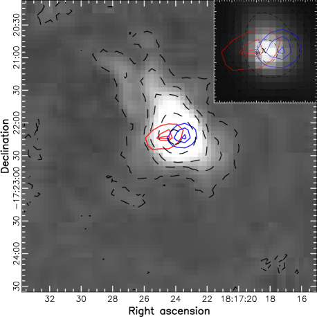
Figure 6: A 4.5′$\times$4.5′field extracted from the SCUBA2 850$\mu$m map. The dashed black contours show flux densities of 12, 3, 1, 0.5 and 0.1 mJy arcsec^-2 respectively on the 850$\mu$m map. The blue and red contours are generated from the CO(3–2) intensity maps of the blue- and red-shifted lobes of the outflow detected in our JCMT+HARP observations, integrated in velocity ranges of 23.3 – 44.0 km s^-1 and 50.6 – 71.3 km s^-1 respectively. The blue contours are at 51, 40 and 25 K km s^-1 and the red contours are at 34.5, 30 and 15 K km s^-1. A 1′$\times$1′image of the central source is shown in high contrast in the inset. ‘$\ast$’ shows the location of source ‘A’ and ‘$\times$’ shows the location of source ‘B’.

Table 6: Flux density of ‘A+B’ measured in different circular apertures from our SCUBA2 maps

Aperture diameter	F   lux density (Jy)
(arcsec)	450 $\mu$m	850 $\mu$m
30	66.6	5.8
40	82.2	7.4
45	87.9	8.0
60	99.6	9.3
80	109.4	10.4
160	120.1	11.8

2.7 Heterodyne observations using HARP

2.7.1 CO ($J$=3–2) data

We obtained heterodyne mapping observations in CO with the JCMT on 20140731 UT. The observations were performed using HARP (Buckle et al., 2009) as the front end and the ASCIS autocorrelator as the back end, in position-switched raster-scan mode with quarter array spacing. ¹²CO (3–2) (345.796 GHz) and H¹³CN (345.3398 GHz), and ¹³CO (3–2) (330.588 GHz) and C¹⁸O (3–2) (329.331 GHz) were simultaneously observed in two different dual sub-band settings of ASCIS. This gives a bandwidth of 250 MHz and a resolution of 61 kHz (0.055 km s^-1) for each line. The scans were performed in a 3$\arcmin\times$3$\arcmin$ area. The CSO $\tau_{225\,GHz}$ was 0.12 for ¹²CO/H¹³CN observations, and 0.128 for ¹³CO/C¹⁸O observations. The pointing accuracy on source is better than 2″.

The data were reduced using the oracdr pipeline, which performs a quality-assurance check on the time-series data, followed by trimming and de-spiking, and an iterative baseline removal routine before creating the final group files. After binning to a resolution of 0.423 km s^-1 (please see the next paragraph), we achieve an RMS noise level of 0.32, 0.31, 0.81 and 1.27 K in ¹²CO, H¹³CN, ¹³CO and C¹⁸O respectively.

We also downloaded JCMT archival data in ¹²CO (3–2), ¹³CO (3–2) and C¹⁸O (3–2) lines. The ¹²CO observations were performed on 20080419 UT with a 1000 MHz band width 2048 channel set up giving a velocity resolution of 0.423 km s^-1. The CSO $\tau_{225\,GHz}$ was 0.115. The ¹³CO and C¹⁸O lines were observed on 20080706 UT in a single setting with 250 MHz band width 4096 channels for each line, giving a velocity resolution of 0.055 and 0.056 km s^-1 respectively. Similar to our observations, the archival observations were also obtained in position-switched raster scan mode, albeit with half array spacing. The CSO $\tau_{225\,GHz}$ was 0.09 for the ¹³CO/C¹⁸O observations. These spectra were binned to a 0.423 km s^-1 resolution as in the ¹²CO line. The ¹²CO, ¹³CO and C¹⁸O archival spectra reached an RMS noise level of 0.41, 0.56 and 0.88 K respectively.

We used our new ¹²CO observations for the figures presented in this paper. Column densities were estimated separately from our own observations and the archival observations to show the repeatability, and the average was used in the discussions. The results from the analysis of the CO data are presented in §3.1.1. No H¹³CN line emission was detected in our observation.

2.7.2 HCO⁺ (4-3)

Archival data of IRAS 18144 in the HCO⁺ (4-3) line (356.7 GHz) were downloaded from the JCMT science archive at CADC. The observations were performed on 20100405 UT with HARP in jiggle map mode covering a field of 2′$\times$2′. A 256 MHz 4096 channel HARP setup was used giving a velocity resolution of 0.051 km s^-1. The mean atmospheric opacity at 225 GHz, measured with the CSO dipper, was 0.084 for the period of the observations. The archival data was reduced using oracdr, further reduction was carried out using kappa. After binning the velocity resolution down to 0.423 km s^-1, we get an RMS of 0.11 K. Fig. 7 shows the spectrum (at the peak) after binning.

Figure 7: The HCO⁺ line at the peak, binned down to a velocity resolution of 0.42 km s^-1. The vertical line shows the systemic velocity of 47.3 km s^-1. The peak T_mb observed was 5.17 K (T${}_{A}^{*}$=3.31)

3 Results and discussions

3.1 The outflow

3.1.1 From the sub-mm data

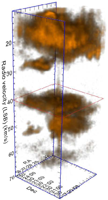
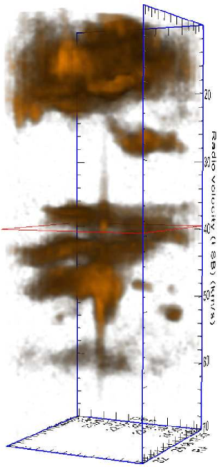
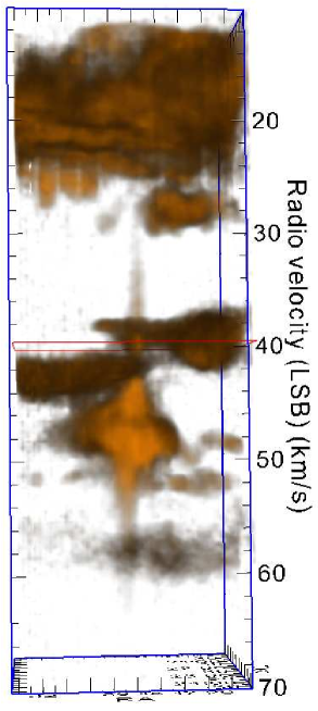
Figure 8: Three different orientations of the ¹²CO (3–2) spectral cube obtained on 20140731 UT showing the outflow, and the emission from the ambient and line-of-sight regions. The images cover a field of 5′$\times$5′ and a radial velocity range of 10–70 km s^-1.

Figure 9: Channel maps of the ¹²CO (3–2) spectral cube shown in Fig. 8. The maps cover a field of 5′$\times$5′ and a radial velocity range of 29.7–64.6 km s^-1. The central velocity of each channel is shown on the uppper left. The contour levels are 1.5–9 K in steps of 1.5 K(T${}_{A}^{*}$).

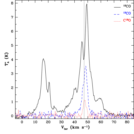
Figure 10: The CO(3–2) spectra extracted and averaged in a 43.7″$\times$43.7″field. The solid black line shows the ¹²CO and the dashed blue line shows the ¹³CO spectra, both from our observations on 20140731 UT. The dotted red line shows the C¹⁸O spectrum; the archival data observed on 20080706 UT is presented for C¹⁸O as it has lower noise. The vertical line shows the systemic velocity of 47.3 km s^-1. The peak T_mb observed for the ¹²CO line was 23.09 K (T${}_{A}^{*}$=14.78 K).

Our observations detect a bipolar CO outflow in this region for the first time. Fig. 8 shows a section extracted from the ¹²CO spectral datacube observed on 20140731 UT showing the outflow and the emission from the ambient and line-of-sight regions. A 5′$\times$5′field in a radial velocity range of 10–70 km s^-1 is shown in the figure. The red square shows a plane at 47.3 km s^-1, the line-of-sight radial velocity of IRAS 18144. Fig. 9 shows a channel map of the same area, in a radial velocity range of 29.7–64.6 km s^-1. From the integrated red-wing, we derive an average outflow diameter of 43″at 3 $\sigma$ above the background level. Therefore, for the purpose of our calculations a spectral cube of 6$\times$6 pixels (43.7″$\times$43.7″) dominated by emission from the central source and the outflow is used. Fig. 10 shows the ¹²CO, ¹³CO and C¹⁸O(3–2) spectra averaged over this region. The ¹²CO emission from the core is optically thick near the line centre and suffers from self absorption. The contours generated from the blue- and red-shifted lobes of the outflow mapped in CO (after integrating in the velocity ranges given below) are overplotted on the continuum-subtracted H₂ image in Fig. 1. The CO outflow is in the E-W direction and it traces the outflow detected in H₂, with the blue-shifted lobe of the CO outflow seen upwind of the MHO 2302 bow-shaped feature, which probably marks the end of the flow lobe.

Figs. 8, 9 and 10 reveal the outflow centered at the systemic velocity, and the emission from the ambient and line-of-sight clouds. Assuming that the emission close to the line centre is mostly contributed by the core, to obtain the emission from the outflow, we integrated the ¹²CO(3-2) spectra from 23.3 to 44.0 km s^-1 on the blue wing, and from 50.6 to 71.3 km s^-1 on the red wing of the outflow. The broad feature with emission peaks centered at 16.1, 20.8 and 25.5 km s^-1 appear to be from the line of sight clouds, and the features at 40 and 58.5 km s^-1 are due to emission and absorption by line-of-sight clouds. These features were interpolated out before integrating the ¹²CO(3-2) spectrum to estimate the emission from the outflow line wings. For the velocity range of integration for estimating the emission from the outflow lobes, we set the velocity of the ¹³CO spectrum where the emission drops to less than 25% of the intenstity at the peak as the inner limit. The outer limits of integration is set where the ¹²CO emission merges with the noise. The integrated intensities from the blue- and red-shifted lobes of the outflow are given in columns 2 and 3 respectively of Table 7.

The optical depth in ¹²CO ($\tau_{12}$) is often estimated from a ratio of the antenna temperatures (T${}^{*}_{A}$) obtained in ¹²CO and ¹³CO asuming ¹²CO/¹³CO = 89 (Garden et al., 1991). Fig. 10 shows that most of the emission from ¹³CO is from the core. Any extended line wing emission in ¹³CO is hard to measure due to noise, which makes the estimate of $\tau_{12}$ from the line ¹²CO/¹³CO ratio highly uncertain. We, therefore, assumed optically thin ¹²CO emission in line wings and adopted the limit of $\tau\,\rightarrow$ 0 in the line wings of the ¹²CO emission. Following Garden et al. (1991) and Varricatt et al. (2013), the ¹²CO column density is then derived using the equation

$$N_{CO}=\frac{2.39\times 10^{14}}{16.6}\frac{e^{\frac{hBJ(J+1)}{kT\textsubscript{ex}}}}{(J+1)}\frac{(T\textsubscript{ex}+0.92)}{e^{\frac{-16.6}{T\textsubscript{ex}}}}\int\frac{T^{*}_{A}}{\eta_{b}}d\upsilon~{}cm^{-1}$$ (1)

where B is the rotational constant, $J$ is the lower level of the transition, and $T$_ex is the excitation temperature.

Table 7: ¹²CO (3–2) line intensities and total H₂ column densitites derived for the blue- and red-shifted lobes of the outflow.

UT Date	$\int T^{*}_{A}$dv (K km s-1)		Column density(cm-2)
(yyyymmdd)	Blue	Red	Blue	Red
20140731	20.75	24.90	1.48$\times 10^{20}$	1.78$\times 10^{20}$
20080419	20.33	23.0	1.45$\times 10^{20}$	1.65$\times 10^{20}$

Adopting 30 K for $T$_ex (Beuther et al., 2002b) and $10^{4}$ for H₂/CO, we estimate 1.46$\times$10²⁰ cm^-2 and 1.71$\times$10²⁰ cm^-2 respectively for the average column density of H₂ in the blue- and red-shifted lobes. Table 7 gives the column densities derived for the red- and blue-shifted lobes of the outflow observed on the two epochs.

The mass in the outflow is estimated using the relation $m\times n_{H_{2}}\times S$, where m is the mean atomic weight, which is 1.36 $\times$ mass of the hydrogen molecule, and S is the surface area of the outflow lobe (Garden et al., 1991). As the ¹²CO column densities were derived from the spectra averaged over a 43.7″$\times$43.7″field, we multiplied the column densities in the two lobes with the same area. Adopting a distance of 4.33 kpc, we estimate outflow masses of 2.67 M_⊙ and 3.13 M_⊙ respectively in the blue- and red-shifted wings, and a total mass of 5.8 M_⊙ in the outflow. Using a mean velocity outflow $v_{mean}$=13.65 km s^-1 with respect to the v_lsr of the core for both red- and blue-shifted lobes in the wavelength range of the outflow lobes considered here, we estimate an outflow momentum of 79.5 M_⊙ km s^-1 and energy of 1.08$\times$10⁴⁶ ergs. The mass we estimate in the outflow is within the range, but towards the lower end of the outflow mass typically estimated for massive YSOs (Beuther et al., 2002b; Zhang et al., 2005).

Note that our estimate of the mass in the outflow should be treated as a lower limit only. The calculations are based adopting $\tau\rightarrow$ 0. An increase in $\tau$ to 10 will inrease the mass, momentum and energy of the outflow by about a factor of 10.

3.1.2 From the near-IR data

In the 2.122 $\mu$m H₂ line (Fig. 1), we obtain a deeper detection of the outflow knot MHO 2302 previously detected by Varricatt et al. (2010). 44 GHz class I methanol maser emission is a good tracer of outflows from massive YSOs. Observations by Gómez-Ruiz et al. (2016) detected 11 maser spots from this region. Nine of those are located within 5″of the H₂ knot MHO 2302 and agree well with the position of the blue shifted lobe of the outflow detected by us in CO. Note that these maser spots are at velocities close to the v_lsr of the core; this suggests that these masers trace post-shock gas in the outflows (Gómez-Ruiz et al., 2016).

The spectrum of the outflow lobe MHO 2302 is given in the lower panel of Fig. 5. Table 5 gives the intensities measured by fitting Gaussians to the lines. The near-IR spectrum of the outflow shows only the emission lines from molecular hydrogen. Except for the 2-1 S(1) line at 2.24 $\mu$m, we don’t see any emission lines from the vibrational states of H₂ higher than $v$=1 suggesting a low level of excitation. Line intensities in Table 5 give a low value of 0.15 for $\frac{2-1S(1)}{1-0S(1)}$; this low value can originate from either non-dissociative shock-excited gas, fluorescently excited low-density gas, or UV heated high density (10⁴–10⁵ cm^-1) gas (Gredel, 1994; Sternberg & Dalgarno, 1989). However, emission from fluorescent excitation will show H₂ from rotational levels with $\upsilon>$3 (Sternberg & Dalgarno, 1989). While the low line ratio alone will not let us conclude that the H₂ emission is shock-excited, lack of any high-$\upsilon$ lines strongly suggest a shock-excitation as the emission mechanism. In addition, we don’t see the 1.644 $\mu$m FeII line in the outflow which suggests a low level of ionization and that the $H_{2}$ emission lines detected are from magnetically-cushioned low-ionization C-type shocks rather than dissociative J-type shocks (O’Connel et al., 2005). However, note that the extinction also is high (A${}_{V}\sim$15.6), so we cannot rule out a non-detection due to extintion.

Under local thermodynamic equilibrium, the column density N($\upsilon$,J) is proportional to the statistical weight $g$ and the Boltzman’s factor $e^{\frac{-E(\upsilon,J)}{kT_{ex}}}$, where E($\upsilon$,J) is the excitation energy, $T_{ex}$ is the excitation temperature and $k$ is the Boltzmann’s constant. If the rotational and vibrational states are thermally coupled, we should get a straight line with a slope $T_{ex}^{-1}$ when we plot $ln(\frac{N(\upsilon,J)}{g})$ against the excitation energy (excitation digram). Following Gredel (1994), the column density can be estimated using the equation:

$$I(\upsilon,J)$=$\frac{hc}{4\pi\lambda}\,A(\upsilon,J)\,N(\upsilon,J)$$ (2)

where I($\upsilon$,J) is the specific intensity of the line, $h$ is the Plank’s constant and A($\upsilon$,J) is the Einstein’s spontaneous emission coefficient. I($\upsilon$,J) have been extinction corrected following the near-IR extinction law derived by Cardelli, Clayton & Mathis (1989), and adopting R_V=A_V/E(B-V)=5.0. Foreground interstellar extinction can also be determined by by iteratively varying A_V and minimizing the scatter around the straight line fit and thus maximizing the goodness of the fit.

Fig. 11 shows the excitation diagram plotted for the lines detected in our spectrum. The straight line fit yields a shock excitation temperature of 2440 K. This value is similar to the excitation temperatures derived for shocked H₂ emission for outflows from massive YSOs (Davis et al., 2004; Caratti o Garatti et al., 2015). We derive a foreground extinction $A_{V}$=15.6 towards the H₂ emission feature.

Figure 11: The excitation diagram for the $H_{2}$ lines measured from the spectrum of MHO 2302. The open circles are from the measured line intensities after extinction correction. The straight line shows a linear fit to the data points.

3.2 The central sources and their natal cloud

Our high angular resolution infrared observations reveal for the first time that the central source of IRAS 18144 is double. The two sources are are labelled ‘A’ and ‘B’ in Figs. 2 and 3. Source ‘A’ was the object previously known as the YSO driving the outflow (Varricatt et al., 2010). It is deeply embedded and is detected well in $K$ band only, with a marginal detection in $H$. Table 8 shows a compilation of the $K$-band photometry available for this source. In $H$ band, we detect a faint point source associated with a cometary nebula. We estimated the photometry in $H$ band using a 1.2″-diameter aperture to avoid as much of the contribution from the nebula as possible, and applying aperture correction. The $H$-band magnitudes are also presented in Table 8. Fig. 12 shows the variations in the $H$ and $K$ magnitudes and the $H$-$K$ colours. We see that source ‘A’ brightened by $\sim$1.2 mag in $K$ during a period of 15 years from 1999 to 2004. Our most recent observations in 2017 and 2018 show that the ‘A’ is fading now. A search by Contreras Peña et al. (2014) in the UKIDSS GPS (Galactic Plane Survey) data of a limited area of the surveyed region with two epochs of $K$-band photometry available suggested that stellar variability with $\Delta\,K$ > 1 mag is very rare. They proposed that most of these high amplitude variables are YSOs. Eruptive YSOs have been classified into FU Ori variables, which exhibit a fast brightening associated with sudden increase in accreation rate followed by a slow decline over a period of over 10 years, or staying in the stage of elevated accretion for decades, and Exor variables, which have recurrent short-lived ($<$1 year) outbursts separated by a few years of quiescence (Contreras Peña et al., 2014; Audard et al., 2014). Both these phenomena are seen in low luninosity objects. With the brightening happening during $\sim$15 years, source ‘A’ does not fall into the category of currently classified eruptive pre-main sequenced variables. Fig. 12 shows that the reddening is lowest when the source is brightest in $H$ and $K$ suggesting that variable amount of obscuration by dust is a major contributor to the variability.

Table 3 shows the flux densities of sources ‘A’ and ‘B’ measured in different Michelle filters. ‘A’ shows variability well above the 1$\sigma$ error limits in all Michelle filters. The variations are suggestive of a fading from 2004 to 2016 and a re-brightening. However, these variations are less than 3$\sigma$. ‘B’ does not exibit any variability above the 1$\sigma$ error limits.

Table 8: $H$ and $K$-band magnitudes of source ‘A’

Data	UT	H		K
source		mag	error	mag	error
DENIS	19980823.06580			11.47c	0.120
2MASS	19990502.36941			11.55c	0.049
UFTI	20030528.57279			11.136d	0.005
WFCAMa	20060718.46093	15.46	0.02
WFCAMa	20060718.46600			10.824	0.001
WFCAMb	20140620.44216	14.93	0.02
WFCAMb	20140620.44627			10.337	0.010
WFCAMb	20140620.44822			10.324	0.010
WFCAMb	20140621.45545	14.94	0.02
WFCAMb	20140621.46008			10.356	0.010
WFCAMb	20170522.56375	15.18	0.02
WFCAMb	20170522.56840			10.591	0.010
WFCAMb	20180330.62079	15.29	0.02
WFCAMb	20180330.62546			10.675	0.010

• From the UKIDSS survey; ^bThis work; ^cAfter conversion to UKIRT-WFCAM system using the $J$-band detection limit of our WFCAM observations; ^dDerived from the $K$-band image of Varricatt et al. (2010)

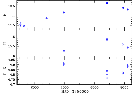
Figure 12: $H$ and $K$ magnitudes, and the $H-K$ colours of source ‘A’, plotted against the Heliocentric Julian Date of observations.

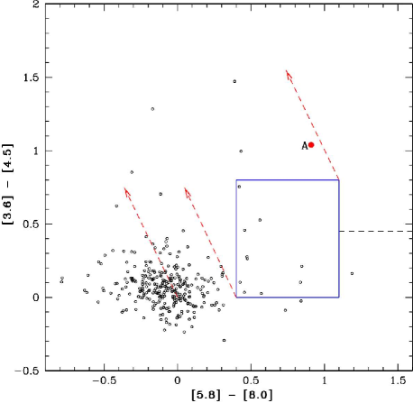
Figure 13: Colour-colour diagram of the objects detected in all IRAC bands in a 10′$\times$10′ field centred on IRAS 18144 (open circles). The filled red circle shows source ‘A’. The blue rectangle shows the approximate location of Class II sources, and the dashed horizontal line shows the boundary between Class I/II objects (below) and Class I objects (above). The dashed red arrows show reddening vectors for A_V = 45.

Spitzer IRAC colours can be used to classify YSOs using the scheme defined by Allen et al. (2004) and Megeath et al. (2004). IRAC ([5.8]-[8.0], [3.6]-[4.5]) colours of objects detected in a 10′$\times$10′ field around IRAS 18144 are plotted in Fig. 13. A majority of the detections are around ([5.8]-[8.0], [3.6]-[4.5]) = 0. These are mostly foreground and background stars and diskless pre-main-sequence (Class III) objects. The blue rectangle (0 < ([3.6]-[4.5]) < 0.8 and 0.4 < ([5.8]-[8.0] < 1.1) shows the approximate location of Class II objects, and the dashed horizontal line shows the boundary between Class I/II (below) and Class I objects (above). The sources with ([3.6]-[4.5]) > 0.8 and ([5.8]-[8.0]) > 1.1 are likely to be Class I objects, which are protostars with infalling envelopes. The dashed red arrows show reddening vectors for A_V = 45 calculated from the extinction law given in Mathis (1990). Sources ‘A’ and ‘B’ are not resolved well in all Spitzer bands, and ‘B’ is not detected in bands 1 and 2. As the 5.8 and 8.0 $\mu$m magnitudes of ‘A’ in the Spitzer catalogue may be influenced by the close proximity of ‘B’, we performed aperture phtometry of ‘A’ from the IRAC images in these two bands, using the mean zero points estimated from a few isolated point sources in the field and adopting a 3″-diamter aperture. We derive magnitudes of 4.95$\pm$0.06 and 4.04$\pm$0.05 respectively in the 5.8 and 8 $\mu$m bands, which are used to derive its [5.8]-[8.0] colour. The location of source ‘A’ in Fig. 13 suggests that it is very young, and is likely to be a reddened Class II object. With ‘B’ being fainter and not resolved well in the Spitzer images, it is difficult to place it in this diagram. Using its flux density measured in the UIST $M^{\prime}$ and Michelle 7.9 $\mu$m bands, approximating the SED with a linear relation, and using the Spitzer-IRAC zero points, we estimate [5.8]-[8.0]$\sim$1.8. This will place ‘B’ in the region of Class I or Class I/II sources in Fig. 13.

The $HK$ spectrum of source ‘A’ (the upper panel of Fig. 5) shows a rising SED, free of photospheric absorption lines suggestive of a YSOs at high extinction. The prominent spectral feature is the Br$\gamma$ emission; we measure an integrated flux of 1.36$\times$10^-17 W m^-2 and an equivalent width of -6.72 Å for this line. Assuming that the Br$\gamma$ line emission is due to accretion, we can use the line strength to obtain an approximate estimate of the accretion rate. The observed line flux was extinction corrected assuming A_V=15.6 towards MHO 2302 derived in §3.1.2 as a lower limit for the extinction towards source ‘A’, and employing the near-IR extinction law derived by Cardelli, Clayton & Mathis (1989). A value of 5 was adopted for R_V. From the extinction corrected flux, we derive a luminosity of 5.51$\times$10^-2 L_⊙ in Br$\gamma$, for a distance of 4.33 kpc. This gives accretion luminosity of 10.2 L_⊙, using the Eq. 2 of Fairlamb et al. (2017). Employing Eq. 11 of Hartigan & Kenyon (2003), and using M_⋆=18 M_⊙ and R_⋆=6.3 R_⊙ from Grave & Kumar (2009) and the accretion luminosity, we estimate an accretion rate of 2.2$\times$10^-5 M_⊙ y^-1 for source ‘A’. Note that this value can have large uncertainty as the A_V could be different towards source ‘A’, and the values of M_⋆ and R_⋆ estimated by Grave & Kumar (2009) could be different from the true values for source ‘A’ as the flux densities used in their SED analysis were the combined values for source ‘A’ and ‘B’.

‘B’ is detected as a deeply embedded source with strong IR colours, and is visible in our images only in $M^{\prime}$ band and at longer wavelengths. Its $M^{\prime}$-band detection is only marginal. It is detected well at longer wavelengths with Michelle, and the Michelle photometry shows a deeper 10 $\mu$m Silicate absorption band than for ‘A’ (Table 3), suggesting that ‘B’ is in a more deeply embedded phase than ‘A’. Source ‘B’ does not exhibit any mid-IR variability above 1$\sigma$. Both ‘A’ and ‘B’ are likely to be YSOs, with ‘B’ in a much younger phase than ‘A’. ‘B’ is probably a Class I or Class I/II object in the envelope phase, where ‘A’ seems to be more advanced Class II object, which has cleared of most of the envelope. With the appearance of ‘B’ as the younger of the two YSOs detected here, its location closer to the centroid of the outflow lobes, and the location of the SCUBA2 and Herschel sources closer to ‘B’ than to ‘A’, we conclude that ‘B’ is the YSO responsible for the outflow seen in CO and H₂, and that it hosts an accretion disk.

The CO(3–2) data can be used to estimate a lower limit to the mass of the cloud. Our CO(3–2) datacube observed on 20140731 UT was integrated in the 32–55 km s^-1 velocity range, the integrated line emission over the whole cloud was extracted and was corrected to the main beam brightness temperature using a main beam efficiency of 0.64 for HARP. We assumed a CO-H₂ conversion factor (X-factor) of 2.0$\times$10²⁰ cm^-2 / K kms^-1 (Bolatto, Wolfire & Leroy, 2013) and a ratio of CO(1–0) to CO(3–2) main beam brightness temperatures of 1.0 (the X-factor is defined for CO J=1–0). We derive a total mass of 3994 M_⊙ for the cloud associated with IRAS 18144. The mass estimate should be treated only as a lower limit to the mass of the cloud as the CO can be underestimated due to optical thickness and feeze out on to dust grains.

The detection of HCO⁺(4-3) (§2.7.2) alone does not allow for an accurate determination of temperature and density in the cloud. However the energy of the $J$=4 level is 43 K above the ground state and therefore it is likely that the kinetic temperature is higher than $\sim$20 K. Molinari et al. (1996) derive a kinetic temperature of 23.61 K from NH₃ observations. Evans (1999) lists the effective density (the critical density, corrected for trapping) needed for the $J$=4-3 transition. It is 5.0$\times$10⁵ cm^-3 for a T_kin of 10 K and 10⁴ cm^-3 for 100 K. The densities are therefore expected to be around 10⁵ cm^-3.

The HCO⁺ emission is slightly elongated EW, with a position angle of 77^∘ and an FWHM of 25.5″$\times$19.5″. This gives a mean radius of 0.24 pc for a distance of 4.33 kpc. After averaging over a 43.7″$\times$47.3″area over which the emission from the core is detected in HCO⁺, we get an FWHM of 4.7 km s^-1 for the line. We can calculate the virial mass of the core following the method adopted by MacLaren, Richardson & Wolfendale (1988) as M=k R $\Delta$V², where M is in solar mass, R is the radius in parsec and $\Delta$V is the FWHM of the line in km s^-1. The value of k is 190 and 126 for a density distribution of r^-1 and r^-2 respectively within the core. This gives us a virial mass of 1007 M_⊙ for an r^-1 density distribution, and 668 M_⊙ for an r^-2 density distribution.

We derive the mass of the cloud from the 850 $\mu$m SCUBA-2 map following Deharveng et al. (2009), using a gas-to-dust ratio of 100. Assuming a dust temperature of 23.61 K, the kinetic temperature derived by Molinari et al. (1996) from NH₃, and a total flux density of 11.8 Jy at 850 $\mu$m (Fig. 6), we obtain a mass of 883 M_⊙. This mass is consistent with the virial mass derived from the HCO⁺(4–3) map, but smaller than the mass derived from ¹²CO(3–2) which is more extended. The core and cloud mass we derive for IRAS 18144 are comparable to the values reported towards other massive YSOs in previous studies (Beuther et al., 2011; Mookerjea et al., 2007).

3.2.1 The spectral energy distribution

The SED of the central source was modelled using the SED fitting tool of Robitaille et al. (2007). This tool uses a grid of 2D radiative transfer models presented in Robitaille et al (2006), and developed by Whitney et al. (2003a) and Whitney et al. (2003b). The grid is composed of 20,000 YSO models, and covers objects in the 0.1–50 M_⊙ range in the evolutionary stages from early envelope infall stage to the late disk-only stage. Each model is available at 10 different viewing angles.

The fit was performed assuming ‘B’ as the sole contributor to the flux densities used. We used the flux density measured in the UIST $M^{\prime}$ band and in the the four Michelle bands. The WISE band W4 data was used, but only as an upper limit as ‘A’ will still be a significant contributor at 22 $\mu$m. AKARI-FIS 65 and 160 $\mu$m fluxes, Herschel measurements from Table 4 and our SCUBA2 measurements from Table 6 were also used for fitting the SED. A mininimum uncertainty of 10% of the observed flux densities was used for observations with smaller uncertainties. Fig. 14 shows the fit to the SED. The solid black line shows the best fit model. The grey lines show the models with $\chi^{2}-\chi^{2}_{bestfit}$ per data point $<$ 3. Our analysis shows a 16.2 M_⊙ star with a disk accretion rate of 9$\times$10^-9 M_⊙/year, envelope accretion rate of 4.25$\times$10${}^{-3}\,$M_⊙/year, total luminosity of 3.07$\times$10${}^{4}\,$L_⊙ and a foreground extinction A_V of 28.7 mag. Table 9 shows the parameters of the best fit model.

SED analysis by Grave & Kumar (2009), derived M=18 M_⊙, age=1.6$\times$10⁵ years, T${}_{*}\sim$20,000 K, M${}_{disk}\sim$0.08 M_⊙, and disk and envelope accretion rates of $\sim$4$\times$10^-6 M_⊙ and $\sim$6.4$\times$10^-5 M_⊙ respectively. Similarly the SED analysis of Tanti, Roy & Duorah (2012) also yielded a 15.44 M_⊙ YSO with age=2.1$\times$10⁴ years, T${}_{*}\sim$14,321 K, and a luminosity of 2.22$\times$10⁴ L_⊙. Sources ‘A’ and ‘B’ were not resolved in these studies. Both these studies and our analysis used the SED fitting tool of Robitaille et al. (2007), with the same underlying models and pre-main-sequence evolutionary tracks.

Whereas the previous studies may have been affected by poor spatial resoltion at all wavelengths, poor resolution at far-IR and sub-mm wavelengths are likely to be affecting our results. Even though the near and mid-IR colours show that ‘B’ as the younger source with a steeper SED when compared to ‘A’, the disk accretion rate for ‘B’ derived from the SED analysis is lower than the the accretion rate for ‘A’ we derive from the Br$\gamma$ luminosity. If ‘B’ is comparable to ‘A’ in mass and is the younger one driving the outflow seen in CO, we expect a larger accretion rate for it.

In general, all disk parameters estimated by the SED fit for ‘B’ have large uncertainty. Note that at near and mid-IR wavelengths, we resolve ‘A’ and ‘B’ and the flux densities of ‘B’ are used in the SED modelling. At longer wavelengths, the spatial resolution is not sufficient to resolve the two sources. The SED modelling is based on the assumption that a single source is responsible for the observed flux densities. Treating the emission at these wavelenghts as entirely from ‘B’ is likely to be significantly affecting the estimation of the disk parameters. If ‘A’ is also a YSO with strong accretion, its contribution in the far-IR and sub-mm wavelengths will not be negligible. Alternatively, ‘B’ itself may be composed of more than one source. We therefore need high angular resolution observations at longer wavelengths to gain better understanding of this system. It should also be noted that the disk accretion rate for embedded sources may not be well-determined due to the fact that the UV accretion luminosity will be reprocessed by absorption and re-emission in the envelope, which has the effect of increasing the total luminosity of the source while not changing the shape of the SED.

Table 9: Results from SED fitting

Parameter	Best-fit valuesa
Stellar mass (M⊙)	16.2 (15.6–21.3)
Stellar radius (R${}_{\odot})$	6.4 (6.4–70.3)
Stellar temperature (K)	3.03 (0.8–3.63)$\times$104
Stellar age (yr)	4.09 (0.83–6.60)$\times$104
Disk mass (M⊙)	4.72 (0.0–133)$\times$10-3
Disk accretion rate (M⊙yr-1)	9 (0.0–167600)$\times$10-9
Disk/Envelope inner radius (AU)	46.7 (0.0–50.4)
Disk outer radius (AU)	5312 (0.0–5312)
Envelope accretion rate (M⊙yr-1)	4.25 (2.25–5.59)$\times$10-3
Envelope outer radius (AU)	1.00 $\times$105
Angle of inclination of the disk axis (∘)	31.8 (31.8–56.6)
Total Luminosity (L⊙)	3.07 (1.81–6.24)$\times$104
AV (foreground)	28.7 (4.0–41.0)

• There were seven other models with ($\chi^{2}-\chi^{2}_{bestfit}$) per data point $<$ 3. The values given in parenthesis are the ranges in the parameter values for all these models. A distance of 4.33 kpc is adopted for IRAS 18144.

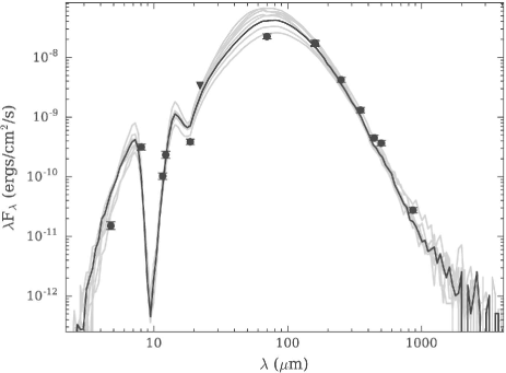
Figure 14: The black line shows the best fit model to the data points. The grey line shows the only other model with $\chi^{2}-\chi^{2}_{bestfit}$ per data point $<$ 3.

4 Conclusions

1. Our sub-mm observations of IRAS 18144 reveal massive star formation taking place in a dense core located in an isolated molecular cloud.

2. We discover an E–W outflow in the CO(3–2) line. The CO outflow is aligned with the jet imaged by us in the 2.122 $\mu$m H₂ line from this region showing that the outflow is jet-driven. We estimate a lower limit of 5.8 M_⊙ for the mass in the outflow.

3. Analysis of the near-IR spectrum of the jet discovered in H₂ gives and excitation temperature of 2440 K and a foreground extinction of A_V=15.6 mag for the H₂ line emission lobe.

4. Through near- and mid-IR imaging, we discover that IRAS 18144 hosts at least two massive YSOs (labelled ‘A’ and ‘B’) in a dense core mapped at 450 and 850 $\mu$m. The newly discovered embedded source ‘B’ is younger and is likely to be the one driving the outflow seen in CO and H₂. Both sources appear to be accreting, and are likely to be in class II and class I stages respectively.

5. The $HK$ spectrum of source ‘A’ shows a steeply rising SED, with Br_γ emission, which is typical of a YSO with accretion. Assuming that the Br_γ emission is from the accretion disk, we calculate an accretion rate of 2.2$\times$10^-5 M_⊙ year^-1.

6. Source ‘B’ is resolved well from ‘A’ in our mid-IR observations. The spatial resolution of the far-IR and sub-mm data are not sufficient to resolve the two sources. Assuming that ‘B’ is the sole contributor to the emission observed at far-IR and sub-mm wavelengths, we modelled the SED, which revealed a 16.2 M_⊙ YSO with a luminosity of 3.07$\times$10⁴ L_⊙. The disk parameters exhibited from the SED analysis have large uncertainties. It is likely that our assumption that ‘B’ is the sole contributor to the observed flux densities at longer wavelengths is not justified, and that the contribution from source ‘A’, at those wavelengths cannot be neglected. Even though the two sources appear close at 2.6″, they have a projected separation of 11258 AU at a distance of 4.33 kpc. We also cannot ignore the possiblity of ‘B’ being composed of more than one source, which are not resolved in our observations. High angular resolution observations at far-IR and sub-mm wavelengths are required to reliably estimate the parameters of the YSOs, and to learn if there are more YSOs associated with this cloud.

7. An examination of the near-IR magnitudes available for source ‘A’, spanning a period of $\sim$20 years, show that source brightened by over 1.1 magnitudes and is now fading. The variation of $H-K$ suggests that the variability is due to varying amount of obscuration by circumstellar dust.

8. We conclude that IRAS 18144 hosts at least two massive YSOs, located inside a dense core situated in an isolated cloud. We estimate a virial mass of 1007 M_⊙ for the core from archival HCO⁺(4–3) data. This is comparable to a mass of 883 M_⊙ derived from our SCUBA-2 850 $\mu$m observations. The SCUBA-2 continuum maps and HCO⁺(4–3) maps show the densest region of the cloud (core) where the two YSOs are located. From our ¹²CO(3-2) data, we estimate a lower limit of 3994 M_⊙ for the mass of the cloud hosting the core.

References

- Allen et al. (2004) Allen L. E. et al. 2004, ApJS, 154, 363
- Arce et al. (2007) Arce H. G., Shepherd D., Gueth F., et al., 2007, Protostars and Planets V, 245
- Audard et al. (2014) Audard M., et al., 2014, in Protostars and Planets VI, eds. H. Beuther, R. S. Klessen, C. P. Dullemond & T. Henning, prpl.conf, 387
- Beuther et al. (2002a) Beuther H., Schilke P., Menten K. M., Motte F., Sridharan T. K., Wyrowski F., 2002a, ApJ, 566, 945
- Beuther et al. (2002b) Beuther H., Schilke P., Sridharan T. K., Menten K. M., Walmsley C. M., Wyrowski F., 2002b, A&A, 383, 892
- Beuther et al. (2011) Beuther H., Linz H., Henning Th., Bik A., Wyrowski F., Schuller F., Schilke P., Thorwirth S., Kim K.-T., 2011, A&A, 531, A26
- Bolatto, Wolfire & Leroy (2013) Bolatto A. D., Wolfire M., Leroy A. K., 2013, ARA&A, 51, 207
- Buckle et al. (2009) Buckle J. V. et al., 2009, MNRAS, 399, 1026
- Cardelli, Clayton & Mathis (1989) Cardelli J. A., Clayton G. C., Mathis J. S., 1989, ApJ, 345, 245
- Casali et al. (2007) Casali M. et al., 2007, A&A, 467, 777
- Cavanagh et al. (2008) Cavanagh B., Jenness T., Economou F., Currie M. J. 2008AN, 329, 295
- Chaplin et al. (2013) Chapin E. L., Berry D. S., Gibb A. G., Jenness T, Scott D., Tilanus R. P. J., Economou F., Holland W. S., 2013, MNRAS, 430, 2545
- Caratti o Garatti et al. (2015) Caratti o Garatti A., Stecklum B., Linz H., Garcia Lopez R., Sanna A., 2015, A&A, 573, 82
- Contreras Peña et al. (2014) Contreras Peña C. et al., 2014, MNRAS, 439, 1829
- Deharveng et al. (2009) Deharveng L., Zavagno A., Schuller F., et al., 2009, A&A 496, 177
- Currie et al. (2008) Currie M. J., Draper P. W., Berry D. S., Jenness T., Cavanagh B., Economou F. 2008, in Argyle R. W., Bunclark P. S., Lewis J. R., eds., Astron. Soc. of the Pac. Conf. Series Vol. 394, Astronomical Data Analysis Software and Systems XVII. p. 650
- Davis et al. (2011) Davis C. J., Cervantes B., Nisini B., Giannini T., Takami M., et al., 2011, A&A, 528, 3
- Davis et al. (2004) Davis C. J., Varricatt W. P., Todd S. P., Ramsay Howat S. K., 2004, A&A, 425, 981
- Dempsey et al. (2013) Dempsey J. T. et al., 2013, MNRAS, 430, 2534
- Evans (1999) Evans II N. J., 1999, ARAA 37, 311
- Fairlamb et al. (2017) Fairlamb J. R., Oudmaijer R. D., Mendigutia I., Ilee J. D., van den Ancker M. E., 2017, MNRAS, 464, 4721
- Fazio et al. (2004) Fazio, G. G. et al. 2004, ApJS, 154, 10
- Fernandex, Brand & Burton (1997) Fernandes A. J. L., Brand P. W. J. L., Burton M. G., 1997, MNRAS, 290, 216
- Garden et al. (1991) Garden R. P., Hayashi M., Hasegawa T., Gatley I., Kaifu N., 1991, ApJ, 374, 540
- Glasse, Atad-Ettedgui & Harris (1997) Glasse, A. C., Atad-Ettedgui, E. I., Harris, J. W. 1997, SPIE, 2871, 1197 (Proc. SPIE Vol. 2871, p. 1197-1203, Optical Telescopes of Today and Tomorrow, Arne L. Ardeberg; Ed.)
- Gómez-Ruiz et al. (2016) Gómez-Ruiz A. I., Kurtz S. E., Araya E. D., Hofner P., Loinard L. 2016, ApJS, 222,18
- Krumholz, McKee & Klein (2005) Krumholz M. R., McKee C. F., Klein R. I., 2005, ApJ, 618, L33
- Grave & Kumar (2009) Grave J. M. C., Kumar M. S. N. 2009, A&A, 498, 147
- Gredel (1994) Gredel R., 1994, A&A, 292, 580
- Griffin et al. (2010) Griffin M. et al., 2010, A&A, 518, 3
- Hartigan & Kenyon (2003) Hartigan P., Kenyon S. J., 2003, ApJ, 583, 334
- Hambly et al. (2008) Hambly N. C., Collins R. S., Cross N. J. G., and 14 co authors 2008, MNRAS, 384, 637
- Hewett et al. (2006) Hewett P. C., Warren S. J., Leggett S. K., Hodgkin S. T., 2006, MNRAS, 367, 454
- Hodgkin et al. (2009) Hodgkin S. T., Irwin M. J., Hewett P. C., Warren S. J., 2009, MNRAS, 394, 675
- Holland et al. (2013) Holland W. S. et al., 2013, MNRAS, 430, 2513
- Irwin et al. (2004) Irwin M. J., Lewis J., Hodgkin S., et al., 2004, in Optimizing Scientific Return for Astronomy through Information Technologies, eds. P. J. Quinn & A. Bridger, Proc. SPIE, 5493, 411
- Kurtz et al. (2004) Kurtz S., Hofner P., Álvarez C. V., 2004, ApJS, 155, 149
- Lada & Lada (2003) Lada C. J., Lada E. A., 2003, ARA&A, 41, 57
- MacLaren, Richardson & Wolfendale (1988) MacLaren I., Richardson K. M., Wolfendale A. W., 1988, ApJ, 333, 821
- Megeath et al. (2004) Megeath S. T. et al. 2004, ApJS, 154, 367
- Molinari et al. (1996) Molinari, S., Brand, J., Cesaroni, R., Palla, F. 1996, A&A, 308, 573
- Molinari et al. (1998) Molinari S., Brand J., Cesaroni R., Palla F., Palumbo G. G. C., 1998, A&A, 336, 339
- Mookerjea et al. (2007) Mookerjea B., Sandell G., Stutzki J., Wouterloot J. G. A, 2007, A&A 473, 485
- Murakami et al. (2007) Murakami H., Baba H., Barthel P., et al. 2007, PASJ, 59, S369
- Muzerolle, Hartmann and Calvet (1998) Muzerolle J., Hartmann L., Calvet N., ApJ, 116, 2965
- O’Connel et al. (2005) O’Connell B., Smith M. D., Froebrich D., Davis C. J., Eislöffel J., 2005, A&A, 431, 223-234
- Palla et al. (1991) Palla F., Brand J., Cesaroni R., Comoretto G., Felli M., 1991, A&A, 246, 249
- Poglitsch et al. (2010) Poglitsch A. et al., 2010, A&A, 518, L2
- Ramsay Howat et al. (2004) Ramsay Howat S. K. et al., 2004, “The commissioning of and first results from the UIST imager spectrometer”, In Proc Spie 5492, Ground-based Instrumentation for Astronomy, eds. A. F. M. Moorwood & I. Masanori, p.1160
- Rice, Wolk & Aspin (2012) Rice T. S., Wolk S. J., Aspin C., 2012, ApJ, 755, 65
- Rieke et al. (2004) Rieke G. H., Young E. T., Engelbracht C. W., et al. 2004, ApJS, 154, 25
- Robitaille et al (2006) Robitaille T. P., Whitney B. A., Indebetouw R., Wood K., and Denzmore P., 2006, ApJS, 167, 256
- Robitaille et al. (2007) Robitaille T. P., Whitney B. A., Indebetouw R., Wood K., 2007, ApJS, 169, 328
- Sternberg & Dalgarno (1989) Sternberg A., Dalrarno A., 1989, ApJ, 338, 197
- Szymczak et al. (2000) Szymczak M., Hrynek G., Kus A. J., 2000, A&AS, 143, 269
- Tanti, Roy & Duorah (2012) Tanti K. K, Roy J., Duorah K., 2012, Adv. Astron. Space Phys., 2, 139
- Varricatt et al. (2010) Varricatt W. P., Davis C. J., Ramsay S., Todd S. P. 2010, MNRAS, 404, 661
- Varricatt et al. (2013) Varricatt W. P., Thomas H. S., Davis C. J., Ramsay S., Currie M. J. 2013, A&A, 554, A9
- Whitney et al. (2003a) Whitney B. A., Wood K., Bjorkman J. E., Cohen M., 2003a, ApJ, 598, 1079
- Whitney et al. (2003b) Whitney B. A., Wood K., Bjorkman J. E., Wolff M. J., 2003b, ApJ, 591, 1049
- Wright et al. (2010) Wright E. L., Eisenhardt P. R. M., Mainzer A. K., et al. 2010, AJ, 140, 1868
- Yamamura et al. (2010) Yamamura, I., Makiuti, S., Ikeda, N., Fukuda, Y, Oyabu, S, Koga, T., White, G. J. 2010, AKARI-FIS Bright Source Catalogue Release note Version 1.0
- Zhang et al. (2005) Zhang Q., Hunter T. R., Brand J., Sridharan T. K., Cesaroni R., Molinari S., Wang J., Kramer M., 2005, ApJ, 625, 864