Dynamical suppression of spacetime torsion

Abstract

A surprising feature of our present four dimensional universe is that its evolution appears to be governed solely by spacetime curvature without any noticeable effect of spacetime torsion. In the present paper, we give a possible explanation of this enigma through “cosmological evolution” of spacetime torsion in the backdrop of a higher dimensional braneworld scenario. Our results reveal that the torsion field may had a significant value at early phase of our universe, but gradually decreased with the expansion of the universe. This leads to a negligible footprint of torsion in our present visible universe. We also show that at an early epoch, when the amplitude of the torsion field was not suppressed, our universe underwent through an inflationary stage having a graceful exit within a finite time. To link the model with observational constraints, we also determine the spectral index for curvature perturbation ($n_{s}$) and tensor to scalar ratio ($r$) in the present context, which match with the results of $Planck$ 2018 (combining with BICEP-2 Keck-Array) data [1].

1 Introduction

A surprising feature of the present universe is that its large scale behaviour appears to be controlled by one type of geometrical deformation only, namely curvature; while we notice practically no effect of another type of deformation, namely torsion. The most straightforward way of including torsion is to add an antisymmetric component to the connection $\Gamma^{\alpha}_{\mu\nu}$, which is the essence of the so-called Einstein-Cartan theory [2]. Once torsion enters into the theory in this manner, it can in principle couple with all matter fields having non zero spin. From dimensional argument, it can be easily shown that such interaction terms in general are of dimension 5, and are suppressed by the Planck mass ($M_{p}$), just as in the case of graviton couplings. But there has been no experimental evidence of the footprint of spacetime torsion on the present universe. An example is the Gravity Probe B experiment which was designed to estimate the precession of a gyroscope to observe any signature of spacetime torsion [3]. However, all such probes, within the limit of their experimental precision, have consistently produced negative results and thereby disfavored the presence of the torsion in the spacetime geometry of our (3 + 1) dimensional visible universe [4, 5, 6]. Therefore the apparent torsion free universe indicates that the torsion field, if exists, must be severely suppressed at the present scale of the universe. Thus the question that naturally arises is : why are the effects of spacetime torsion are less perceptible than the spacetime curvature ? There is no satisfactory answer to this in the domain of four dimensional classical gravity models.
The proposals to remove torsion by quantum effects in 4 dimensional spacetime have appeared much before in [7], where the authors showed the invisibility of spacetime torsion (on the present energy scale of our universe) through the consideration of quantum corrected (caused by vacuum effects) gravitational action with torsion. There was also attempts to seek an answer to this in the context of higher dimensional braneworld models [8, 9, 10, 11, 12, 13, 14]. In particular, in Randall-Sundrum (RS) scenario [10] which involves one extra compact spacelike dimension with $S^{1}/Z_{2}$ orbifolding along the extra dimension proposed a possible explanation for this suppression of spacetime torsion in four dimension. This kind of scenario postulates gravity in the five-dimensional ‘bulk’, whereas our four-dimensional universe is confined to one of the two 3-branes located at the two orbifold fixed points along the compact dimension. However it has been already shown that a rank-2 antisymmetric tensor field, generally known as Kalb-Ramond (KR) field ($B_{MN}$), can act as a source of spacetime torsion where the torsion is identified with rank-3 antisymmetric field strength tensor $H_{MNL}$ having a relation with $B_{MN}$ as $H_{MNL}=\partial_{[M}B_{NL]}$ [15]. In the RS like scenario where both the gravity and the KR field propagate in the bulk, the exponential warping nature of spacetime geometry causes the KR field (or equivalently the torsion) to be diluted on the visible 3-brane [8, 16, 17, 18]. Also there is a recent work on spacetime torsion with antisymmetric tensor fields in higher curvature gravity model in the context of both four dimensional and five dimensional spacetime [19], where the authors showed that due to the effect of higher curvature term(s), the amplitude of torsion field gets suppressed in the course of the universe evolution.
However in the background of cosmological evolution, the suppression of spacetime torsion (on our present universe) sourced by Kalb-Ramond field still awaits a proper understanding. Furthermore one of our authors showed earlier that the amplitude of KR field may be significant and can play a relevant role in the early phase of the universe. This motivates to explore whether the “dynamical evolution” of KR field (from early universe) actually leads to a negligible footprint of torsion on the present universe in the backdrop of braneworld scenario. We also want to explore the “cosmological evolution” of KR field from very early universe to examine whether the universe underwent through an inflationary expansion [20, 21, 22, 23, 24, 25, 26, 27]. In particular, the questions that we address in the present paper are :

• How does the Kalb-Ramond field evolve from early era of our universe? Does this evolution lead to an explanation of why the effect of torsion is so much weaker than that of curvature on the present visible brane?

• In such circumstance, does the four dimensional universe undergo an accelerating expansion at early epoch? If such an inflationary scenario is allowed, then what is the dependence of the duration of inflation on the KR field energy density? Moreover what are the values of the spectral index ($n_{s}$) and tensor to scalar ratio ($r$) in the present context?

The present paper serves a natural explanation of the above questions in the backdrop of Randall-Sundrum scenario. However the warped RS geometry in its original form is intrinsically unstable due to intervening bulk gravity. A popular way of stabilizing the interbrane separation (also known as modulus or radion) is via Goldberger-Wise (GW) mechanism [28, 29] which proposes the existence of a bulk stabilizing scalar field. Some variants of RS model and its modulus stabilization are discussed in [14, 30, 31, 32, 33, 34, 35, 36]. Following the GW mechanism, here we propose a dynamical stabilization method of the extra dimensional modulus field (coupled to the KR field through the effective field equations).
Our paper is organized as follows: the model is described in section-II, while section-III is reserved for presenting the cosmological field equations and their possible solutions from the perspective of four dimensional effective theory. Their implications and possible consequences are discussed in the remaining part of the paper.

2 The model

We consider a five dimensional compactified warped geometry two brane model with spacetime torsion in the bulk. In the present context, the source of torsion is taken as rank-2 antisymmetric Kalb-Ramond (KR) field $B_{MN}$ (where latin indices run from $0$ to $4$). Torsion can be identified with rank-3 antisymmetric field strength tensor $H_{MNL}$ which is related to the KR field as $H_{MNL}=\partial_{[M}B_{NL]}$. The spacetime is $S^{1}/Z_{2}$ orbifolded along the extra dimension, where the orbifolded fixed points are identified with two 3-branes. Considering $\phi$ as extra dimensional angular coordinate, two branes are located at $\phi=0$ (hidden brane) and at $\phi=\pi$ (visible brane) respectively while the latter one is identified with the visible universe. One of the crucial aspects of this braneworld scenario is to stabilize the distance between the branes (known as modulus or radion). For this purpose, one needs to generate a suitable modulus potential with a stable minima and in order to do this, here we consider a massive scalar field in the five dimensional bulk. Therefore the action of the model is given by,

$$S = \int d^{4}xd\phi\sqrt{-G}\bigg{[}\frac{R^{(5)}}{2\kappa^{2}}-\Lambda+V_{h}\delta(\phi)+V_{v}\delta(\phi-\pi)$$ (1)

$$- \frac{1}{2}G^{MN}\partial_{M}\Psi\partial_{N}\Psi-\frac{1}{2}m^{2}\Psi^{2}-\frac{1}{12}H_{MNL}H^{MNL}\bigg{]}$$

where $R^{(5)}$ is the five dimensional Ricci scalar formed by the metric $G_{MN}$, $\frac{1}{2\kappa^{2}}=M^{3}$ ($M$ is the 5 dimensional Planck mass), $\Lambda(<0)$ is the bulk cosmological constant and $V_{h}$, $V_{v}$ are the brane tensions on hidden, visible brane respectively. $\Psi$ is the stabilizing scalar field with $m$ denoting its mass. The KR field action is represented by the last term in the above action.
Considering a negligible backreaction of the KR field ($B_{MN}$) and the scalar field ($\Psi$) on the background spacetime, the solution of metric $G_{MN}$ turns out to be same as well known RS model i.e

$$ds^{2}=e^{-2kr_{c}\phi}\eta_{\mu\nu}dx^{\mu}dx^{\nu}+r_{c}^{2}d\phi^{2}$$ (2)

where $k=\sqrt{\frac{-\Lambda}{24M^{3}}}$ and $r_{c}$ is the interbrane separation. With this metric, the scalar field equation of motion in the bulk is following,

$$\frac{1}{r_{c}^{2}}\frac{\partial}{\partial\phi}\bigg{[}e^{-4kr_{c}\phi}\frac{\partial\Psi}{\partial\phi}\bigg{]}-m^{2}e^{-4kr_{c}\phi}\Psi(\phi)=0$$ (3)

where $\Psi$ is taken as the function of $\phi$ only. Considering non-zero value of $\Psi$ on the branes, the above eqn.(3) has the general solution,

$$\Psi(\phi)=e^{2kr_{c}\phi}\bigg{[}Ae^{\sigma kr_{c}\phi}+Be^{-\sigma kr_{c}\phi}\bigg{]}$$ (4)

where $\sigma=\sqrt{4+\frac{m^{2}}{k^{2}}}$. Further the integrations constants $A$ and $B$ are obtained from the boundary conditions, $\Psi(0)=v_{h}$ and $\Psi(\pi)=v_{v}$ as follows,

$$A = v_{v}e^{-(\sigma+2)kr_{c}\pi}-v_{h}e^{-2\sigma kr_{c}\pi}$$

$$B = v_{h}\big{(}1+e^{-2\sigma kr_{c}\pi}\big{)}-v_{v}e^{-(\sigma+2)kr_{c}\pi}$$ (5)

Using the five dimensional spacetime metric (see eqn.(2)), different components of stress tensor of the stabilizing scalar field ($\Psi$) can be obtained as,

$$T_{\phi\phi}(\Psi)=\frac{1}{4}r_{c}^{2}\bigg{[}-\frac{1}{r_{c}^{2}}(\partial_{\phi}\Psi)^{2}+m^{2}\Psi^{2}\bigg{]}\\$$

and

$$T_{\mu\nu}(\Psi)=e^{-2kr_{c}\phi}\eta_{\mu\nu}\frac{1}{4}\bigg{[}\frac{1}{r_{c}^{2}}(\partial_{\phi}\Psi)^{2}+m^{2}\Psi^{2}\bigg{]}\\$$

Putting the bulk scalar field solution (eqn. 3) in the expression of $T_{\phi\phi}(\Phi)$ and $T_{\mu\nu}(\Phi)$ and using the form of $A$ and $B$ in terms of $v_{v}$ and $v_{h}$ (eqn. 5), one can show that the ratio of corresponding component of stress tensor between bulk scalar field and bulk cosmological constant varies as $v_{v}^{2}/M^{3}$ i.e

$$\bigg{(}\frac{T_{\phi\phi}(\Psi)}{T_{\phi\phi}(\Lambda)}\bigg{)}\sim v_{v}^{2}/M^{3}~{}~{}~{}~{}~{},~{}~{}~{}~{}~{}~{}\bigg{(}\frac{T_{\mu\nu}(\Psi)}{T_{\mu\nu}(\Lambda)}\bigg{)}\sim v_{v}^{2}/M^{3}$$

where $T_{\phi\phi}(\Lambda)$ and $T_{\mu\nu}(\Lambda)$ are different components of stress tensor for the bulk cosmological constant. Similarly the Lagrangian density for Kalb-Ramond field leads to the ratio of KR field stress tensor with the bulk cosmological constant as $\sim H_{MNL}H^{MNL}/M^{5}$. Thus the stress tensor for the bulk scalar field as well as for the KR field is less than that of the bulk cosmological constant for $v_{v}^{2}/M^{3}$ and $H_{MNL}H^{MNL}/M^{5}$ less than unity. These conditions allow us to neglect the backreaction of the stabilizing scalar field and the KR field (on the background spacetime) in comparison to bulk cosmological constant.
In order to introduce the radion field, we consider a fluctuation of branes around the stable configuration ($r_{c}$). So, the interbrane separation can be considered as a field ($T(x)$) and here, for simplicity, we assume that this new field depends only on the brane coordinates. The corresponding metric ansatz is,

$$ds^{2}=e^{-2kT(x)\phi}g_{\mu\nu}(x)dx^{\mu}dx^{\nu}+T(x)^{2}d\phi^{2}$$ (6)

Correspondingly the introduction of radion field leads to the bulk scalar field ($\Psi$) solution as follows,

$$\Psi(x,\phi)=e^{2kT(x)\phi}\bigg{[}Ae^{\sigma kT(x)\phi}+Be^{-\sigma kT(x)\phi}\bigg{]}$$ (7)

where $A$ and $B$ are given by the following expressions,

$$A = v_{v}e^{-(\sigma+2)kT(x)\pi}-v_{h}e^{-2\sigma kT(x)\pi}$$

$$B = v_{h}\big{(}1+e^{-2\sigma kT(x)\pi}\big{)}-v_{v}e^{-(\sigma+2)kT(x)\pi}$$

Having these set-up, now we proceed to obtain the effective four dimensional action leading to a viable physical description of our visible universe. In the following few subsections, we individually determine the explicit form of 4D effective action for various parts of the original five dimensional action (eqn.(1)).

2.1 Effective action for 5D Einstein-Hilbert term

With the metric in eqn.(6), a Kaluza-Klein reduction for the five dimensional Einstein-Hilbert action reduces to four dimensional effective action as,

$$S_{eff}^{(1)}=\int d^{4}x\sqrt{-g}\bigg{[}\frac{M^{3}}{k}R^{(4)}-\frac{12M^{3}}{k}g^{\mu\nu}\partial_{\mu}\bigg{(}e^{-k\pi T(x)}\bigg{)}\partial_{\nu}\bigg{(}e^{-k\pi T(x)}\bigg{)}\bigg{]}$$ (8)

where $R^{(4)}$ is the four dimensional Ricci scalar formed by the on-brane metric $g_{\mu\nu}$. As it is evident that $T(x)$ is not canonical and thus we redefine the field by the following transformation :

$$T(x)\longrightarrow\xi(x)=\sqrt{\frac{24M^{3}}{k}}e^{-k\pi T(x)}$$ (9)

In terms of the canonical radion field $\xi(x)$, $S_{eff}^{(1)}$ takes the following form,

$$S_{eff}^{(1)}=\int d^{4}x\sqrt{-g}\bigg{[}\frac{M^{3}}{k}R^{(4)}-\frac{1}{2}g^{\mu\nu}\partial_{\mu}\xi\partial_{\nu}\xi\bigg{]}$$ (10)

2.2 Effective action for bulk scalar field ($\Psi$): Radion potential

Plugging the bulk scalar field solution (see eqn.(7)) back into the five dimensional scalar field action $S_{scalar}=\int d^{4}xd\phi\sqrt{-G}\big{[}-\frac{1}{2}G^{MN}\partial_{M}\Psi\partial_{N}\Psi-\frac{1}{2}m^{2}\Psi^{2}\big{]}$ and integrating over the extra dimensional coordinate $\phi$ yields the effective action as follows,

$$S_{eff}^{(2)}=\int d^{4}x\sqrt{-g}\bigg{[}-\frac{k^{3}}{144M^{6}}\xi^{4}\bigg{(}v_{h}(\xi/f)^{\sigma}-v_{v}\bigg{)}^{2}\bigg{]}$$ (11)

where $f=\sqrt{\frac{24M^{3}}{k}}$. Further to derive the above expression, we use the relation between $T(x)$ and $\xi(x)$ as shown in eqn.(9). However it may be noticed that the integrand of eqn.(11) acts as a potential term for the radion field. Afterwards we denote this potential by $V(\xi)$ i.e

$$V(\xi)=\frac{k^{3}}{144M^{6}}\xi^{4}\bigg{(}v_{h}(\xi/f)^{\sigma}-v_{v}\bigg{)}^{2}$$ (12)

Eqn.(12) clearly indicates that the potential $V(\xi)$ goes to zero in absence of the bulk scalar field (i.e $v_{h}=v_{v}=0$). Therefore as mentioned earlier, the potential term for the radion field is generated entirely due to the presence of the bulk scalar field $\Psi$ [28, 29].
The potential in eqn.(12) has a minimum at

$$\xi_{min} = <\xi>$$ (13)

$$= f\bigg{[}\frac{v_{v}}{v_{h}}\bigg{]}^{1/\sigma}$$

and a maxima at

$$\xi_{max}=f\bigg{[}\frac{v_{v}}{v_{h}}\bigg{(}\frac{2}{2+\sigma}\bigg{)}\bigg{]}^{1/\sigma}$$ (14)

respectively. Moreover $V(\xi)$ goes to zero as $\xi=0$. In figure [1] we give a plot of $V(\xi)$ against $\xi$. With the expression of $<\xi>$, we determine the squared mass of the radion field as

$$m_{rad}^{2}=\frac{k^{2}v_{v}^{2}\sigma^{2}}{3M^{3}}\bigg{(}\frac{v_{v}}{v_{h}}\bigg{)}^{2/\sigma}$$ (15)

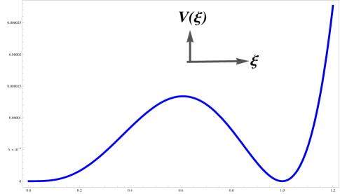
Figure 1: $V(\xi)$ vs $\xi$

2.3 Effective action for KR field action

Recall that the 5D KR field action is given by,

$$S_{H}=-\frac{1}{12}\int d^{4}xd\phi\sqrt{-G}\bigg{[}H_{MNL}H^{MNL}\bigg{]}$$ (16)

where the KR field strength tensor $H_{MNL}$ is related to $B_{MN}$ (second rank antisymmetric tensor field) as $H_{MNL}=\partial_{[M}B_{NL]}$, with latin and greek indices running from $0$ to $4$ and $0$ to $3$ respectively. It is easy to see that the action $S[H]$ is invariant under the gauge transformation as $B_{MN}\rightarrow B_{MN}+\partial_{M}\omega_{N}$ (with $W_{N}$ as an arbitrary function of spacetime coordinates). This gauge invariance of KR field allows us to set $B_{4\mu}=0$. Using the form of $G_{MN}$ (see eqn.(6)) and keeping $B_{4\mu}=0$, the above action turns out to be,

$$S_{H} = -\frac{1}{12}\int d^{4}xd\phi\sqrt{-g}e^{2kT(x)\phi}T(x)\bigg{[}g^{\mu\alpha}g^{\nu\beta}g^{\lambda\gamma}H_{\mu\nu\lambda}H_{\alpha\beta\gamma}$$ (17)

$$- \frac{3}{T(x)^{2}}e^{-2kT(x)\phi}g^{\mu\alpha}g^{\nu\beta}B_{\mu\nu}\partial_{\phi}^{2}B_{\alpha\beta}\bigg{]}$$

The Kaluza-Klein decomposition for the KR field can be written as,

$$B_{\mu\nu}(x,\phi)=\sum B_{\mu\nu}^{(n)}(x)\chi^{(n)}(x,\phi)$$ (18)

where $B_{\mu\nu}^{(n)}(x)$ and $\chi^{(n)}(x,\phi)$ represent the $n$th mode of on-brane KR field and extra dimensional KR wave function respectively. It may be mentioned that the wave function $\chi^{(n)}$ is considered to be a function of brane coordinates also (apart from the coordinate $\phi$), this is because our motive is to investigate whether the “dynamical evolution” of KR field leads to its invisibility on our present universe.
Substituting the decomposition in the 5-dimensional action $S_{H}$ and integrating over the extra dimension, the four dimensional effective action turns out to be:

$$S_{eff}^{(3)} = -\frac{1}{12}\int d^{4}x\sqrt{-g}\bigg{[}g^{\mu\alpha}g^{\nu\beta}g^{\lambda\gamma}H_{\mu\nu\lambda}^{(n)}H_{\alpha\beta\gamma}^{(n)}$$ (19)

$$+ 3m_{n}^{2}g^{\mu\alpha}g^{\nu\beta}B_{\mu\nu}^{(n)}B_{\alpha\beta}^{(n)}\bigg{]}$$

provided $\chi^{(n)}(x,\phi)$ satisfies the following equation of motion,

$$\frac{\partial\chi^{(n)}}{\partial t}\frac{\partial\chi^{(m)}}{\partial t}-\frac{1}{T^{2}(t)}e^{-2kT(t)\phi}\chi^{(n)}\frac{\partial^{2}\chi^{(m)}}{\partial\phi^{2}}=m_{n}^{2}\chi^{(n)}\chi^{(m)}$$ (20)

along with the normalization condition as,

$$\int_{0}^{\pi}d\phi e^{2kT(t)\phi}\chi^{(n)}\chi^{(m)}=\frac{1}{T^{2}(t)}\delta_{mn}$$ (21)

where $m_{n}$ denotes the mass of nth KK mode. As we will see later that $\chi^{(n)}(x,\pi)$ is important to determine the coupling between the KR field and various Standard Model fields on the visible brane. Further eqn.(20) clearly demonstrates that the dynamical evolution of $\chi^{(n)}(x,\phi)$ is coupled with the modulus (or radion) field $T(x)$.

Eqns.(10), (11) and (19) immediately lead to the final form of the four dimensional effective action as follows :

$$S_{eff} = S_{eff}^{(1)}+S_{eff}^{(2)}+S_{eff}^{(3)}$$ (22)

$$= \int d^{4}x\sqrt{-g}\bigg{[}\frac{M^{3}}{k}R^{(4)}-\frac{1}{2}g^{\mu\nu}\partial_{\mu}\xi\partial_{\nu}\xi-V(\xi)$$

$$+ g^{\mu\alpha}g^{\nu\beta}g^{\lambda\gamma}H_{\mu\nu\lambda}^{(n)}H_{\alpha\beta\gamma}^{(n)}+3m_{n}^{2}B_{\mu\nu}^{(n)}B^{\mu\nu(n)}\bigg{]}$$

where the radion potential $V(\xi)$ is explicitly shown in eqn.(12). At this stage it deserves mentioning that the zeroth Kaluza-Klein (KK) mode of the field strength tensor (i.e $H^{(0)}_{\mu\nu\lambda}$) can be identified with spacetime torsion and thus from now on, we deal with the zeroth mode of the KR field for which $m_{n=0}=0$. With this lowest KK mode, the four dimensional effective action turns out to be,

$$S_{eff} = S_{eff}^{(1)}+S_{eff}^{(2)}+S_{eff}^{(3)}$$ (23)

$$= \int d^{4}x\sqrt{-g}\bigg{[}\frac{M^{3}}{k}R^{(4)}-\frac{1}{2}g^{\mu\nu}\partial_{\mu}\xi\partial_{\nu}\xi-V(\xi)$$

$$+ g^{\mu\alpha}g^{\nu\beta}g^{\lambda\gamma}H_{\mu\nu\lambda}^{(0)}H_{\alpha\beta\gamma}^{(0)}\bigg{]}$$

However due to the presence of the potential $V(\xi)$, the radion field acquires a certain dynamics governed by the effective field equations. In this scenario, our motivation is to investigate whether the dynamics of the radion field can trigger such a evolution on the KR wave function $\chi^{(0)}(x,\phi)$, that will lead to the fact that the effect of KR field (or equivalently the torsion field) evolves to get suppressed with the expansion of our universe. Further in [18], it was shown that the energy density of $B^{(0)}_{\mu\nu}$ may be dominant and can have a significant role at early phase of the universe. Therefore it is crucial to explore the dynamical evolution of KR field from very early era of the universe where it is also an intriguing part to examine whether the early universe passes through an inflationary period or not. Motivated by this idea, we try to solve the cosmological Freidmann equations obtained from the four dimensional effective action $S_{eff}$. This is demonstrated in the next section.
At this stage it deserves mentioning that the energy scale, or the compactification scale, of the five dimensional bulk is $\sim$ Planck scale. However as mentioned earlier that here we are interested on inflation on our 4D visible universe, where the energy scale (or the inverse of the duration of inflation) comes with $\sim 10^{10}$ GeV which is consistent with the Planck observations as has been described later. Thus the 4D inflationary energy scale is lesser compared to the 5D bulk scale and we can consider the 4D effective action where the extra dimensional component of 5D metric i.e the modulus appears as radion field. Thus the approach here is motivated by the calculation of the effective action proposed by Goldberger and Wise in [28, 29].

3 Effective cosmological equations and their possible solutions

In order to obtain the effective field equations, first we determine the energy-momentum tensor for $\xi(x)$ and $B_{\mu\nu}^{(0)}(x)$ as,

$$T_{\mu\nu}[\xi] = \frac{2}{\sqrt{-g}}\frac{\delta}{\delta g^{\mu\nu}}\bigg{[}\sqrt{-g}\bigg{(}\frac{1}{2}g^{\alpha\beta}\partial_{\alpha}\xi\partial_{\beta}\xi+V(\xi)\bigg{)}\bigg{]}$$ (24)

$$= \partial_{\mu}\xi\partial_{\nu}\xi-g_{\mu\nu}\bigg{(}\frac{1}{2}g^{\alpha\beta}\partial_{\alpha}\xi\partial_{\beta}\xi+V(\xi)\bigg{)}$$

and

$$T_{\mu\nu}[B^{(0)}] = \frac{2}{\sqrt{-g}}\frac{\delta}{\delta g^{\mu\nu}}\bigg{[}\frac{1}{12}\sqrt{-g}g^{\mu\alpha}g^{\nu\beta}g^{\lambda\gamma}H_{\mu\nu\lambda}H_{\alpha\beta\gamma}\bigg{]}$$ (25)

$$= \frac{1}{6}\bigg{[}3g_{\nu\rho}H_{\alpha\beta\mu}H^{\alpha\beta\rho}-\frac{1}{2}g_{\mu\nu}H_{\alpha\beta\gamma}H^{\alpha\beta\gamma}\bigg{]}$$

respectively.
The on-brane metric ansatz that fits our purpose is the flat FRW metric i.e

$$ds_{(4)}^{2} = g_{\mu\nu}(x)dx^{\mu}dx^{\nu}$$ (26)

$$= -dt^{2}+a^{2}(t)\big{[}dx^{2}+dy^{2}+dz^{2}\big{]}$$

where $a(t)$ is the scale factor of the visible universe. However before presenting the field equations, we want to emphasize that due to antisymmetric nature, $H_{\mu\nu\lambda}^{(0)}$ has four independent components on the visible 3-brane, they can be expressed as,

$$H_{012}^{(0)}=h_{1}~{}~{}~{}~{}~{}~{}~{}~{}~{}~{}~{}~{},~{}~{}~{}~{}~{}~{}~{}~{}~{}~{}~{}~{}H^{012(0)}=h^{1}$$

$$H_{013}^{(0)}=h_{2}~{}~{}~{}~{}~{}~{}~{}~{}~{}~{}~{}~{},~{}~{}~{}~{}~{}~{}~{}~{}~{}~{}~{}~{}H^{013(0)}=h^{2}$$

$$H_{023}^{(0)}=h_{3}~{}~{}~{}~{}~{}~{}~{}~{}~{}~{}~{}~{},~{}~{}~{}~{}~{}~{}~{}~{}~{}~{}~{}~{}H^{023(0)}=h^{3}$$

$$H_{123}^{(0)}=h_{4}~{}~{}~{}~{}~{}~{}~{}~{}~{}~{}~{}~{},~{}~{}~{}~{}~{}~{}~{}~{}~{}~{}~{}~{}H^{123(0)}=h^{4}$$

With these independent components along with the metric shown in eqn.(26), we determine various components of $T_{\mu\nu}[\xi]$ and $T_{\mu\nu}[B^{(0)}]$, as given in Appendix-1. Such expressions of energy-momentum tensor immediately lead to the off-diagonal Friedmann equations (obtained from the effective action $S_{eff}$ in eqn.(23)) as,

$$h_{4}h^{3}=h_{4}h^{2}=h_{4}h^{1}=h_{2}h^{3}=h_{1}h^{3}=h_{1}h^{2}=0$$ (27)

The above set of equations has the following solution,

$$h_{1}=h_{2}=h_{3}=0~{}~{}~{}~{}~{}~{}~{}~{}~{}~{}~{}~{}~{}~{}~{}~{}~{},h_{4}\neq 0$$ (28)

Using this solution, one easily obtains total energy density and pressure for the matter fields ($\xi$, $B_{\mu\nu}^{(0)}$) as $\rho_{T}=\bigg{[}\frac{1}{2}\dot{\xi}^{2}+V(\xi)+\frac{1}{2}h_{4}h^{4}\bigg{]}$ and $p_{T}=\bigg{[}\frac{1}{2}\dot{\xi}^{2}-V(\xi)+\frac{1}{2}h_{4}h^{4}\bigg{]}$ respectively (where the fields are taken to be homogeneous in space and an overdot denotes $\frac{d}{dt}$). As a result, the diagonal Friedmann equations take the following form,

$$3H^{2}=\frac{1}{2}\dot{\xi}^{2}+V(\xi)+\frac{1}{2}h_{4}h^{4}$$ (29)

$$2\dot{H}+3H^{2}+\frac{1}{2}\dot{\xi}^{2}-V(\xi)+\frac{1}{2}h_{4}h^{4}=0$$ (30)

where $H=\frac{\dot{a}}{a}$ is known as Hubble parameter. Further, the effective field equations for the zeroth mode of KR field ($B_{\mu\nu}^{(0)}$) and the radion field ($\xi$) are given by,

$$\nabla_{\mu}H^{\mu\nu\lambda(0)}=\frac{1}{\sqrt{-g}}\partial_{\mu}\bigg{[}\sqrt{-g}H^{\mu\nu\lambda(0)}\bigg{]}=0$$ (31)

and

$$\ddot{\xi}+3H\dot{\xi}+\frac{\partial V}{\partial\xi}=0$$ (32)

respectively, where $V(\xi)$ is explicitly shown in eqn.(12). However the only information that we get from eqn.(31) is that the non-zero component of $H_{\mu\nu\lambda}^{(0)}$ i.e $h_{4}$ depends on the coordinate $t$ (see Appendix-2 for the derivation), as is also expected from the gravitational field equations. Taking time derivative of both sides of eqn.(29), we get $6H\dot{H}=\bigg{[}\dot{\xi}\ddot{\xi}+V^{\prime}(\xi)\dot{\xi}+\frac{1}{2}\frac{d}{dt}(h_{4}h^{4})\bigg{]}$. Further eqns.(29) and (30) immediately lead to an expression as $2\dot{H}=-\dot{\xi}^{2}-\frac{1}{2}h_{4}h^{4}$. Equating these two expressions of $\dot{H}$ and using the radion field equation, one finally lands with the following time evolution for $h_{4}h^{4}$ as,

$$\frac{d}{dt}(h_{4}h^{4})=-6Hh_{4}h^{4}$$

Solving the above differential equation, we obtain

$$h_{4}h^{4}=\frac{h_{0}}{a^{6}(t)}$$ (33)

where $h_{0}$ is an integration constant which is restricted to take only positive values in order to get a real solution of $h_{4}$. Recall that the term $\frac{1}{2}h_{4}h^{4}$ represents the energy density contributed from the KR field i.e $\rho_{KR}=\frac{1}{2}h_{4}h^{4}$. Therefore eqn.(33) clearly indicates that the energy density of the KR field (zeroth mode) decreases monotonically as the universe expands with time. This leads to a negligible footprint of spacetime torsion on our present visible universe. However at the same time eqn.(33) also demonstrates that the energy density of the KR field should play an important role at early phase of the universe (when $a(t)$ is small compared to the present one). Therefore in order to understand the dynamical suppression of the KR field, it is crucial to determine the time evolution of $h_{4}$ from very early universe where it is also important to examine whether the universe undergoes through an inflationary stage or not. To investigate these phenomena, we need to solve the scale factor during initial era.
Using the above form of $h_{4}h^{4}$ (see eqn.(33)), there remain two independent effective field equations,

$$H^{2}=\frac{1}{3}\bigg{[}\frac{1}{2}\dot{\xi}^{2}+V(\xi)\bigg{]}+\frac{1}{6}\frac{h_{0}}{a^{6}}$$ (34)

$$\ddot{\xi}+3H\dot{\xi}+\frac{\partial V}{\partial\xi}=0$$ (35)

These two equations are sufficient to determine the two unknowns namely the scale factor ($a(t)$) and the radion field ($\xi(t)$). As mentioned earlier, we are interested to solve eqns.(34), (35) during early universe and for this purpose, the potential energy of the radion field is considered to be greater than that of the kinetic energy (known as slow-roll approximation) i.e.

$$V(\xi)\gg\frac{1}{2}\dot{\xi}^{2}$$ (36)

Under this approximation, eqn.(34) and eqn.(35) are simplified to,

$$H^{2}=\frac{1}{3}V(\xi)+\frac{1}{6}\frac{h_{0}}{a^{6}}$$ (37)

and

$$3H\dot{\xi}+\frac{\partial V}{\partial\xi}=0$$ (38)

respectively. Using the explicit form of $V(\xi)$ (see eqn. (12)), we solve the above two equations for $\xi(t)$, $a(t)$ as,

$$\xi(t)=\frac{\xi_{0}}{\bigg{[}D\xi_{0}^{\sigma}-\big{(}D\xi_{0}^{\sigma}-\frac{\sqrt{h_{0}}}{a_{0}^{3}\xi_{0}^{2}}-1\big{)}\exp{\big{[}-\frac{1}{3}\sigma v_{v}\sqrt{\frac{k^{3}}{3M^{6}}}(t-t_{0})\big{]}}\bigg{]}^{1/\sigma}}$$ (39)

and

$$a(t)=C\bigg{[}1+\sqrt{\frac{3h_{0}}{2}}(t-t_{0})\bigg{]}^{1/3}\exp{\bigg{[}\frac{1}{12}v_{v}\sqrt{\frac{k^{3}}{3M^{6}}}\big{(}g_{1}(t)-g_{2}(t)\big{)}\bigg{]}},$$ (40)

where $D=\frac{v_{h}}{v_{v}}\big{(}\frac{k}{24M^{3}}\big{)}^{\sigma/2}$ and $\xi_{0}$, $C$ are integration constants with $a_{0}=C\exp{[-\xi_{0}^{2}/8]}$. Further $g_{1}(t)$ has the following form,

$$g_{1} (t)=-\frac{D\xi_{0}^{\sigma}}{(D\xi_{0}^{\sigma}-1)}\bigg{(}\frac{1}{\frac{1}{3}\sigma v_{v}\sqrt{\frac{k^{3}}{3M^{6}}}}\bigg{)}$$ (41)

$$2F1 \bigg{(}1,1,2+\frac{2}{\sigma},\frac{D\xi_{0}^{\sigma}}{D\xi_{0}^{\sigma}-1}\exp{\big{(}\frac{1}{3}\sigma v_{v}\sqrt{\frac{k^{3}}{3M^{6}}}(t-t_{0})\big{)}}\bigg{)}$$

$$\exp {\bigg{(}\frac{1}{3}\sigma v_{v}\sqrt{\frac{k^{3}}{3M^{6}}}(t-t_{0})\bigg{)}}\bigg{(}D\xi_{0}^{\sigma}-(D\xi_{0}^{\sigma}-1)$$

$$\exp {\big{(}-\frac{1}{3}\sigma v_{v}\sqrt{\frac{k^{3}}{3M^{6}}}(t-t_{0})\big{)}}\bigg{)}^{-2/\sigma}$$

where $2F1$ symbolizes the hypergeometric function. Similarly the form of $g_{2}(t)$ is given by,

$$g_{2} (t)=-\frac{\xi_{0}^{\sigma}}{(D\xi_{0}^{\sigma}-1)}\bigg{(}\frac{1}{\frac{1}{3}\sigma v_{v}\sqrt{\frac{k^{3}}{3M^{6}}}}\bigg{)}*$$ (42)

$$2F1 \bigg{(}1,1,1+\frac{2}{\sigma},\frac{D\xi_{0}^{\sigma}}{D\xi_{0}^{\sigma}-1}\exp{\big{(}\frac{1}{3}\sigma v_{v}\sqrt{\frac{k^{3}}{3M^{6}}}(t-t_{0})\big{)}}\bigg{)}$$

$$\exp {\bigg{(}\frac{1}{3}\sigma v_{v}\sqrt{\frac{k^{3}}{3M^{6}}}(t-t_{0})\bigg{)}}\bigg{(}D\xi_{0}^{\sigma}-(D\xi_{0}^{\sigma}-1)$$

$$\exp {\big{(}-\frac{1}{3}\sigma v_{v}\sqrt{\frac{k^{3}}{3M^{6}}}(t-t_{0})\big{)}}\bigg{)}^{1-2/\sigma}.$$

It may be noticed from eqn.(39) and eqn.(40) that for $\Psi\rightarrow 0$ (or $v_{v}=0$), the solution of the radion field and the Hubble parameter become $\xi(t)=\frac{\xi_{0}}{\big{[}1+\frac{\sqrt{h_{0}}}{a_{0}^{3}\xi_{0}^{2}}\big{]}^{1/\sigma}}=\xi(t_{0})$ and $H\propto\frac{1}{a^{3}}$ respectively. This is expected because in the absence of bulk scalar field ($\Psi$), the potential $V(\xi)$ (see eqn.(12)) goes to zero and thus the radion field has no dynamics which in turn makes the variation of the Hubble parameter as $H\propto\frac{1}{a^{3}}$ (solely due to the KR field having equation of state parameter $=1$).
Further eqn.(39) clearly indicates that $\xi(t)$ decreases with time. Comparison of eqn.(13) and eqn.(39) reveals that the radion field reaches at its vacuum expectation value (vev) asymptotically (within the slow roll approximation) at large time ($t\gg t_{0}$) i.e.

$$\Psi(t\gg t_{0}) = f\bigg{[}\frac{v_{v}}{v_{h}}\bigg{]}^{1/\sigma}$$ (43)

$$= <\Psi>$$

This vev of radion field leads to the stabilized interbrane separation (between Planck and TeV branes) as,

$$k\pi<T(x)>=\frac{4k^{2}}{m^{2}}[\ln{(\frac{v_{h}}{v_{v}})}]$$ (44)

where $m^{2}$ is squared mass of the stabilizing scalar field $\Psi$.

4 Beginning of inflation

After obtaining the solution of $a(t)$ (in eqn.(40)), we can now examine whether this form of scale factor corresponds to an accelerating era of the early universe (i.e. $t\gtrsim t_{0}$) or not. In order to check this, we expand $a(t)$ in the form of Taylor series (about $t=t_{0}$) and retain the terms only up to first order in $t-t_{0}$:

$$a(t\gtrsim t_{0})=a_{0}\bigg{[}1+\sqrt{\frac{3h_{0}}{2}}(t-t_{0})\bigg{]}^{1/3}\exp{\bigg{[}\frac{1}{12}\xi_{0}^{2}v_{v}\sqrt{\frac{k^{3}}{3M^{6}}}(D\xi_{0}^{\sigma}-1)(t-t_{0})\bigg{]}}$$ (45)

where $a_{0}$ is the value of the scale factor at $t=t_{0}$ and related to the integration constant $C$ as,

$$a_{0}=C\exp{[-\xi_{0}^{2}/8]}.$$

Eqn.(45) leads to the acceleration of the universe at $t\rightarrow t_{0}$ as follows:

$$\frac{\ddot{a}}{a}(t\gtrsim t_{0} ) =\bigg{[}\frac{\xi_{0}^{2}v_{v}}{12}\sqrt{\frac{k^{3}}{3M^{6}}}(D\xi_{0}^{\sigma}-1)+\sqrt{\frac{h_{0}}{2}}\big{(}1+\frac{1}{\sqrt{3}}\big{)}\bigg{]}$$ (46)

$$\bigg{[} \frac{\xi_{0}^{2}v_{v}}{12}\sqrt{\frac{k^{3}}{3M^{6}}}(D\xi_{0}^{\sigma}-1)-\sqrt{\frac{h_{0}}{2}}\big{(}1-\frac{1}{\sqrt{3}}\big{)}\bigg{]}$$

It may be noticed that for the condition

$$\frac{\xi_{0}^{2}v_{v}}{12}\sqrt{\frac{k^{3}}{3M^{6}}}(D\xi_{0}^{\sigma}-1)>\sqrt{\frac{h_{0}}{2}}\big{(}1-\frac{1}{\sqrt{3}}\big{)}$$ (47)

the early universe undergoes through an accelerating stage while for $\frac{\xi_{0}^{2}v_{v}}{12}\sqrt{\frac{k^{3}}{3M^{6}}}(D\xi_{0}^{\sigma}-1)<\sqrt{\frac{h_{0}}{2}}\big{(}1-\frac{1}{\sqrt{3}}\big{)}$, $\ddot{a}(t\rightarrow t_{0})$ becomes less than zero.
At this stage, it deserves mentioning that the parameters $v_{v}$ and $h_{0}$ controls the strength of the radion field and the KR field energy density respectively. Therefore the interplay between the radion field and the KR field fixes whether the early universe evolves through an accelerating stage or not. However in order to solve the flatness and horizon problems (for a review, we refer to [21, 22]), the universe must passes through an accelerating stage at early epoch and from this requirement, here we stick to the condition shown in eqn.(47).

5 End of inflation and reheating

In the previous section, we show that the very early universe expands with an acceleration and this accelerating stage is termed as the inflationary epoch. In this section, we check whether such acceleration of the scale factor has an end in a finite time or not.
The end point of an inflationary era is defined by,

$$\frac{\ddot{a}}{a}=\dot{H}+H^{2}=0$$ (48)

We now examine whether this condition is consistent with the field equations shown in eqn.(37) and eqn.(38). Near the end of inflation, one can safely neglect the term proportional to $1/a^{6}$ and thus eqn.(37) takes the following form (at end regime of inflation):

$$H^{2} = \frac{1}{3}V(\xi)$$

$$= \frac{k^{3}}{432M^{6}}v_{v}^{2}\xi^{4}\bigg{(}D\xi^{\sigma}-1\bigg{)}^{2}$$

Differentiating both sides of this equation with respect to t, we get the time derivative of the Hubble parameter as follows,

$$\dot{H}=-\frac{k^{3}}{54M^{6}}v_{v}^{2}\xi^{2}\bigg{(}D\xi^{\sigma}-1\bigg{)}^{2}$$ (49)

where we use the equation of the radion field ($3H\dot{\xi}+V^{\prime}(\xi)=0$). Plugging back the expressions of $H^{2}$ and $\dot{H}$ into eqn.(48), one gets the following condition on radion field,

$$\xi=2\sqrt{2}=\xi_{f}=\xi(t_{f})$$ (50)

where $t_{f}$ is the time when the radion field acquires the value $2\sqrt{2}$ (in Planckian unit). Eqn. (50) clearly indicates that the inflationary era of the universe continues as long as the radion field remains greater than $\xi_{f}$ ($=2\sqrt{2}$). Correspondingly the duration of inflation (i.e. $t_{f}-t_{0}$) can be calculated from the solution of $\xi_{(}t)$ as follows,

$$\xi_{f}^{\sigma}=\frac{\xi_{0}^{\sigma}}{\bigg{[}D\xi_{0}^{\sigma}-(D\xi_{0}^{\sigma}-\frac{\sqrt{h_{0}}}{a_{0}^{3}\xi_{0}^{2}}-1)\exp{[-\frac{1}{3}\sigma v_{v}\sqrt{\frac{k^{3}}{3M^{6}}}(t_{f}-t_{0})]}\bigg{]}}$$

Simplifying the above expression, we obtain

$$t_{f}-t_{0}=\bigg{(}\frac{3}{\sigma v_{v}\sqrt{\frac{k^{3}}{3M^{6}}}}\bigg{)}\ln\bigg{[}\frac{D\xi_{0}^{\sigma}-1-\frac{\sqrt{h_{0}}}{a_{0}^{3}\xi_{0}^{2}}}{D\xi_{0}^{\sigma}-\frac{\xi_{0}^{\sigma}}{\xi_{f}^{\sigma}}}\bigg{]}$$ (51)

recall $D=\frac{v_{h}}{v_{v}}\big{(}\frac{k}{24M^{3}}\big{)}^{\sigma/2}$ and $\sigma=\frac{m^{2}}{4k^{2}}$.
Therefore it is clear that the inflation comes to an end in a finite time. In order to estimate the duration of inflation explicitly, one needs the value of the parameters $h_{0}$, $\xi_{0}$ and $v_{v}$, which can be determined from the expressions of spectral index and tensor to scalar ratio as discussed in the next section.
However before moving to the next section, here we discuss the reheating in the present context and the possible effects of KR field (or equivalently the spacetime torsion) on it. Needless to say that reheating describes the production of Standard Model matter at the end of the period of accelerated expansion. For this purpose, we consider an example where the radion field (i.e the inflaton) is coupled to another scalar field $\zeta$, given by the interaction Lagrangian,

$$L_{int}=-g\lambda\xi\zeta^{2}$$ (52)

where $g$ is a dimensionless coupling constant and $\lambda$ is a mass scale. With this interaction Lagrangian, the decay rate of the inflaton into $\zeta$ particles becomes

$$\Gamma=\frac{g^{2}\lambda^{2}}{8\pi m_{rad}}$$ (53)

recall that $m_{rad}$ is the mass of the radion field (see eqn.(15)). Generally the energy loss of the inflaton due to the production of $\zeta$ particles is taken into account by adding a damping term to the inflaton equation of motion as,

$$\ddot{\xi}+3H\dot{\xi}+\Gamma\dot{\xi}+\frac{\partial V}{\partial\xi}=0$$ (54)

Eqn.(54) clearly indicates that the radion field losses energy due to the expansion of the universe and due to transfer to the $\zeta$ particles, accounted by the damping terms $3H\dot{\xi}$ and $\Gamma\dot{\xi}$ respectively. As a result the production of $\zeta$ particles becomes effective when the Hubble parameter becomes less or comparable to $\Gamma$, otherwise the energy loss into particles is negligible compared to the energy loss due to the expansion of space as occurred during early phase of the inflation. Therefore the time scale $t_{h}$ (let us call it the reheating time) after when the production of $\zeta$ becomes effective is given by

$$H(t_{h})=\Gamma$$ (55)

With the solution of scale factor (see eqn.(40)), the above equation turns out to be,

$$\frac{1}{12}v_{v}\sqrt{\frac{k^{3}}{3M^{6}}}\big{(}\dot{g}_{1}(t_{h})-\dot{g}_{2}(t_{h})\big{)}+\frac{\sqrt{\frac{3h_{0}}{2}}}{3\bigg{(}1+\sqrt{\frac{3h_{0}}{2}}t_{h}\bigg{)}}=\Gamma$$ (56)

where $g_{1}$ and $g_{2}$ are shown in eqns.(41) and (42) respectively. Recall, $h_{0}$ represents the energy density of the KR field during early universe and the presence of $h_{0}$ in the above expression entails that the KR field indeed affects the reheating time $t_{h}$. In order to understand the effect of KR field more clearly, we write $t_{h}=t_{h}^{(0)}+\delta t$, where $t_{h}^{(0)}$ is the reheating time in absence of KR field ($h_{0}=0$) i.e

$$\frac{1}{12}v_{v}\sqrt{\frac{k^{3}}{3M^{6}}}\big{(}\dot{g}_{1}(t_{h}^{(0)})-\dot{g}_{2}(t_{h}^{(0)})\big{)}=\Gamma$$ (57)

Thus $\delta t$ is the deviation of reheating time from $t_{h}^{(0)}$ solely due to the presence of the KR field. Expanding eqn.(56) in terms of $t_{h}=t_{h}^{(0)}+\delta t$, we get the following expression of $\delta t$

$$\delta t=-\frac{\sqrt{\frac{3h_{0}}{2}}}{\frac{1}{4}v_{v}\sqrt{\frac{k^{3}}{3M^{6}}}\bigg{(}1+\sqrt{\frac{3h_{0}}{2}}t_{h}^{(0)}\bigg{)}\bigg{(}\ddot{g}_{1}(t_{h}^{(0)})-\ddot{g}_{2}(t_{h}^{(0)})\bigg{)}}$$ (58)

where we use eqn.(57) and retain up to the term first order in $\delta t$. Clearly $\delta t$ becomes zero as $h_{0}\rightarrow 0$, as expected. Using the explicit expressions of $g_{1}$, $g_{2}$ along with the condition $\frac{m}{k}<1$ (i.e ratio of bulk scalar field mass to bulk curvature is less than unity, which is also consistent with Planck observations as described in the next section), we determine the term $\ddot{g}_{1}-\ddot{g}_{2}$ (sitting in the denominator of eqn.(58)) as follows:

$$\ddot{g}_{1}-\ddot{g}_{2} = \bigg{(}\frac{D\xi_{0}^{\sigma}}{(D\xi_{0}^{\sigma}-1)}\bigg{)}^{2}\bigg{(}\frac{\frac{1}{3}\sigma v_{v}\sqrt{\frac{k^{3}}{3M^{6}}}}{\big{(}1+2/\sigma\big{)}\big{(}2+2/\sigma\big{)}}\bigg{)}\bigg{(}D\xi_{0}^{\sigma}-(D\xi_{0}^{\sigma}-1)\exp{\big{(}-\frac{1}{3}\sigma v_{v}\sqrt{\frac{k^{3}}{3M^{6}}}(t-t_{0})\big{)}}\bigg{)}^{-2/\sigma}$$ (59)

$$\bigg{[} 3~{}2F1\bigg{(}2,2,\frac{2}{\sigma},\frac{D\xi_{0}^{\sigma}}{D\xi_{0}^{\sigma}-1}\exp{\big{(}\frac{1}{3}\sigma v_{v}\sqrt{\frac{k^{3}}{3M^{6}}}(t-t_{0})\big{)}}\bigg{)}\exp{\bigg{(}\frac{2}{3}\sigma v_{v}\sqrt{\frac{k^{3}}{3M^{6}}}(t-t_{0})\bigg{)}}$$

$$+ \frac{8}{\big{(}3+2/\sigma\big{)}}2F1\bigg{(}3,3,\frac{2}{\sigma},\frac{D\xi_{0}^{\sigma}}{D\xi_{0}^{\sigma}-1}\exp{\big{(}\frac{1}{3}\sigma v_{v}\sqrt{\frac{k^{3}}{3M^{6}}}(t-t_{0})\big{)}}\bigg{)}\exp{\bigg{(}\sigma v_{v}\sqrt{\frac{k^{3}}{3M^{6}}}(t-t_{0})\bigg{)}}\bigg{]}$$

Thus the term $\ddot{g}_{1}-\ddot{g}_{2}$ is positive. As a result, eqn.(58) immediately leads to the condition $\delta t<0$ which in turn makes $t_{h}<t_{h}^{(0)}$. Thereby the presence of Kalb-Ramond field makes the reheating time lesser in comparison to the case when the KR field is absent. However, this is expected because the KR field corresponds to a deceleration of the universe i.e due to the appearance of KR field the Hubble parameter ($H(t)$) decreases with a faster rate by which $H(t)$ reaches to $\Gamma$ more quickly relative to the situation where the KR field is absent.

6 Spectral index, tensor to scalar ratio and number of e-foldings

In order to test the broad inflationary paradigm as well as particular models against precision observations [1], we need to calculate the value of spectral index($n_{s}$) and tensor to scalar ratio ($r$) and for this purpose, here we define a dimensionless parameter (known as slow roll parameter) as,

$$\epsilon=-\dot{H}/H^{2}$$ (60)

Recall the slow roll equation, $H^{2}=\frac{1}{3}V(\xi)+\frac{h_{0}}{6a^{6}}$. Differentiating both sides of this equation with respect to time, we get

$$2\dot{H}=-\frac{1}{9H^{2}}\bigg{(}\frac{\partial V}{\partial\xi}\bigg{)}^{2}-\frac{h_{0}}{a^{6}}$$

where we use the field equation for radion field. These expressions of $\dot{H}$ and $H^{2}$ lead to the slow roll parameter $\epsilon$ as follows,

$$\epsilon=\frac{1}{2}\bigg{[}\frac{16p^{2}v_{v}^{4}\xi^{6}(D\xi^{\sigma}-1)^{4}+\frac{3h_{0}}{a^{6}}\bigg{(}pv_{v}^{2}\xi^{4}(D\xi^{\sigma}-1)^{2}+\frac{h_{0}}{2a^{6}}\bigg{)}}{\bigg{(}pv_{v}^{2}\xi^{4}(D\xi^{\sigma}-1)^{2}+\frac{h_{0}}{2a^{6}}\bigg{)}^{2}}\bigg{]}$$

(61)

where $p=\frac{k^{3}}{144M^{6}}$ and $D=\frac{v_{h}}{v_{v}}\big{(}\frac{k}{24M^{3}}\big{)}^{\sigma/2}$.
The spectral index and tensor to scalar ratio are defined by,

$$n_{s} = 1-2\epsilon\bigg{|}_{t=t_{0}}-\frac{\dot{\epsilon}}{H\epsilon}\bigg{|}_{t=t_{0}}$$

$$r = 16\epsilon\bigg{|}_{t=t_{0}}$$

With the expression of $\epsilon$ obtained in eqn.(61), $r$ and $n_{s}$ turn out to be,

$$r=8\bigg{[}\frac{16p^{2}v_{v}^{4}\xi_{0}^{6}(D\xi_{0}^{\sigma}-1)^{4}+\frac{3h_{0}}{a_{0}^{6}}\bigg{(}pv_{v}^{2}\xi_{0}^{4}(D\xi_{0}^{\sigma}-1)^{2}+\frac{h_{0}}{2a_{0}^{6}}\bigg{)}}{\bigg{(}pv_{v}^{2}\xi_{0}^{4}(D\xi_{0}^{\sigma}-1)^{2}+\frac{h_{0}}{2a_{0}^{6}}\bigg{)}^{2}}\bigg{]}$$

(62)

and

$$n_{s}=1-\frac{U_{1}}{U_{2}}$$ (63)

where $U_{1}$ and $U_{2}$ have the following expressions:

$$U_{1} = \bigg{[}384p^{3}v_{v}^{6}\xi_{0}^{8}(D\xi_{0}^{\sigma}-1)^{6}+\frac{18h_{0}}{a_{0}^{6}}\bigg{(}pv_{v}^{2}\xi_{0}^{4}(D\xi_{0}^{\sigma}-1)^{2}+\frac{h_{0}}{2a_{0}^{6}}\bigg{)}^{2}$$

$$- \frac{6h_{0}}{a_{0}^{6}}\bigg{(}16p^{2}v_{v}^{4}\xi_{0}^{6}(D\xi_{0}^{\sigma}-1)^{4}+\frac{3h_{0}}{a_{0}^{6}}\bigg{(}pv_{v}^{2}\xi_{0}^{4}(D\xi_{0}^{\sigma}-1)^{2}+\frac{h_{0}}{2a_{0}^{6}}\bigg{)}\bigg{)}$$

$$- \frac{144h_{0}}{a_{0}^{6}}p^{2}v_{v}^{4}\xi_{0}^{6}(D\xi_{0}^{\sigma}-1)^{4}\bigg{]}$$

and

$$U_{2} = \bigg{(}pv_{v}^{2}\xi_{0}^{4}(D\xi_{0}^{\sigma}-1)^{2}+\frac{h_{0}}{2a_{0}^{6}}\bigg{)}\bigg{(}16p^{2}v_{v}^{4}\xi_{0}^{6}(D\xi_{0}^{\sigma}-1)^{4}$$

$$+ \frac{3h_{0}}{a_{0}^{6}}\bigg{(}pv_{v}^{2}\xi_{0}^{4}(D\xi_{0}^{\sigma}-1)^{2}+\frac{h_{0}}{2a_{0}^{6}}\bigg{)}\bigg{)}$$

respectively. It may be observed that the spectral index and tensor to scalar ratio depend on the parameters $v_{v}$, $h_{0}$ and $\xi_{0}$. To fix these parameters, we use the observational results of Planck 2018 ( combining with BICEP-2 Keck-Array data ) [1] which put a constraint on $n_{s}$ and $r$ as $n_{s}=0.9649\pm 0.0042$ and $r<0.064$ respectively. Here we take,

$$\kappa v_{v}=\frac{\sqrt{h_{0}}}{M^{2}}\simeq 10^{-7}.$$

It may be mentioned that these values of $v_{v}$ and $h_{0}$ are consistent with the condition that is necessary for neglecting the backreaction of the bulk scalar field and the KR field on the background five dimensional spacetime.
Using eqns.(63), (62) along with the values of $v_{v}$ and $h_{0}$, we give the plots (see Figure[2], Figure[3]) of $n_{s}$, $r$ with respect to $\xi_{0}$.

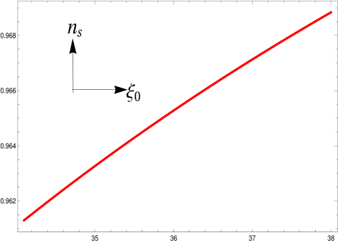
Figure 2: $n_{s}$ vs $\xi_{0}$

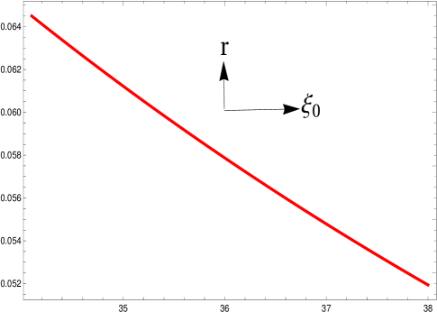
Figure 3: $r$ vs $\xi_{0}$

Figures [2] and [3] clearly demonstrate that for $34<\xi_{0}<38$ (in Planckian unit), both the observable quantities $n_{s}$ and $r$ remain within the constraints provided by $Planck$ 2018 [1].
Further with the estimated values of $v_{v}$, $h_{0}$ and $\xi_{0}$, the duration of inflation ($t_{f}-t_{0}$, see eqn.(51)) comes as $10^{-10}$(Gev)^-1 if the ratio $m/k$ (bulk scalar field mass to bulk curvature ratio) is taken as $0.2$ [28]. We also determine the number of e-foldings, defined by $N=\int_{0}^{\vartriangle t}Hdt$ ($\vartriangle t=t_{f}-t_{0}$, duration of inflation), numerically and lands with $N\simeq 58$ (with $\xi_{0}=36$, in Planckian unit).
In table[1], we now summarize our results:

Parameters	Estimated values
$n_{s}$	$0.969$
$r$	0.100
$t_{f}-t_{0}$	$10^{-10}$(GeV)-1
$N$	58

Table 1: Estimated values of various quantities for $\kappa v_{v}=\frac{\sqrt{h_{0}}}{M^{2}}\simeq 10^{-7}$ and $\xi_{0}=36$

Table[1] clearly indicates that the present model may well explain the inflationary scenario of the universe in terms of the observable quantities $n_{s}$ and $r$ as per the results of $Planck$ 2018.
Using the solutions of $\xi(t)$, $a(t)$ (see eqns.(39), (40)) along with the estimated values of the parameters ($v_{v}$, $h_{0}$, $\xi_{0}$), we give the plots for the interbrane separation ($T(t)$, see figure[4]) and the deceleration parameter ($q=-\ddot{a}/a$, see figure[5]) against a dimensionless time variable $\tilde{t}=\frac{t}{t_{f}}N$.

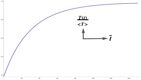
Figure 4: $\frac{T(t)}{<T>}$ vs $\tilde{t}$

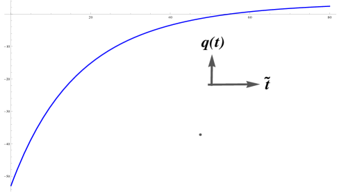
Figure 5: $q(t)$ vs $\tilde{t}$

where we use the relation $\xi(t)=\sqrt{\frac{24M^{3}}{k}}e^{-k\pi T(t)}$. Fig.[4] clearly reveals that the interbrane separation increases with time and saturates at $\frac{4k^{2}}{m^{2}}\ln{[v_{h}/v_{v}]}$ ($=k\pi<T>$, see eqn.(44)) asymptotically. It may be mentioned that for $v_{h}/v_{v}=1.5$ and $m/k=0.2$, $k\pi<T>$ acquires the value $\simeq 36$ - required for solving the gauge hierarchy problem. Further Fig.[5] demonstrates that the early universe starts from an accelerating stage with a graceful exit at a finite time.

7 Solution for Kalb-Ramond extra dimensional wave function

The equation for the zeroth mode of KR wave function ($\chi^{(0)}(t,\phi)$) follows from eqn.(20) and given by,

$$\bigg{(}\frac{\partial\chi^{(0)}}{\partial t}\bigg{)}^{2}-\frac{1}{T^{2}(t)}e^{-2kT(t)\phi}\chi^{(0)}\frac{\partial^{2}\chi^{(0)}}{\partial\phi^{2}}=0$$ (64)

As we may notice that the dynamics of the interbrane separation controls the evolution of $\chi^{(0)}(t,\phi)$.
It may be mentioned that the overlap of $\chi^{(0)}(t,\phi)$ with the brane $\phi=\pi$ (i.e. $\chi^{(0)}(t,\pi)$) regulates the coupling strengths between KR field and various Standard Model fields on the visible brane. These interaction terms play the key role to determine the observable signatures of KR field on our universe and thus we are interested to solve eqn.(64) in the vicinity of $\phi=\pi$ (i.e. near the visible brane). Near the regime of $\phi\simeq\pi$, eqn.(64) can be written as,

$$\bigg{(}\frac{\partial\chi_{v}^{(0)}}{\partial t}\bigg{)}^{2}-\frac{1}{T^{2}(t)}e^{-2k\pi T(t)}\chi_{v}^{(0)}\frac{\partial^{2}\chi_{v}^{(0)}}{\partial\phi^{2}}=0$$ (65)

where $\chi_{v}^{(0)}$ denotes the KR wave function near the visible brane. Eqn.(65) can be solved by the method of separation of variables as $\chi_{v}^{(0)}(t,\phi)=f_{1}(t)f_{2}({\phi})$. With this expression, eqn.(65) turns out to be,

$$T^{2}(t)e^{2k\pi T(t)}\frac{1}{f_{1}^{2}}\bigg{(}\frac{df_{1}}{dt}\bigg{)}^{2}=\frac{1}{f_{2}}\frac{d^{2}f_{2}}{d\phi^{2}}$$ (66)

As it is evident that the left and right hand side of eqn.(66) are functions of time and $\phi$ alone respectively. Therefore both sides of eqn.(66) can be separately equated with a constant as follows:

$$T^{2}(t)e^{2k\pi T(t)}\frac{1}{f_{1}^{2}}\bigg{(}\frac{df_{1}}{dt}\bigg{)}^{2}=b^{2}$$ (67)

and

$$\frac{1}{f_{2}}\frac{d^{2}f_{2}}{d\phi^{2}}=b^{2}$$ (68)

where $b$ is the constant of separation. Solution of eqn.(68) is given by $f_{2}(\phi)=e^{-b\phi}$, while eqn.(67) is solved numerically as shown in Fig.[5] (plotted with respect to the dimensionless time variable $\tilde{t}=\frac{t}{t_{f}}N$, with $N$ be the number of e-foldings of the inflationary era).

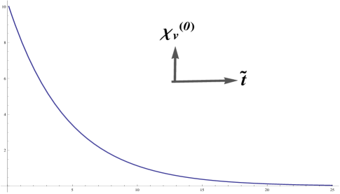
Figure 6: $\chi_{v}^{(0)}$ vs $\tilde{t}$

Fig.[6] clearly demonstrates that in the regime $\phi\simeq\pi$, the KR wave function monotonically decreases with time and the decaying time scale ($\tilde{t}\simeq 25$) is less than the exit time of the inflation ($\tilde{t}=55$). This may explain why the present universe carries practically no observable signatures of the rank two antisymmetric Kalb-Ramond field (or equivalently the torsion field).
Thereby as a whole, the solution of $\chi_{v}^{(0)}(t,\phi)$ is given by $\chi_{v}^{(0)}(t,\phi)=e^{-b\phi}f_{1}(t)$, where $f_{1}(t)$ is obtained in figure[6]. Using this solution as a boundary condition, we solve eqn.(64) (evolution of KR wave function in the whole bulk) numerically as plotted in Fig.[7].

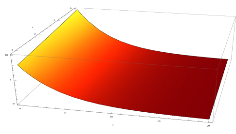
Figure 7: $\chi^{(0)}$ vs $\phi$ (along x axis) and $t$

Fig.[7] reveals that the zeroth mode of KR wave function $\chi^{(0)}(t,\phi)$ decreases with time in the whole five dimensional bulk i.e for $0\leq\phi\leq\pi$. However for a fixed $t$, $\chi^{(0)}(t,\phi)$ has different values (in Planckian unit) on hidden and visible brane and such hierarchial nature of $\chi^{(0)}(t,\phi)$ (between the two branes) is controlled by the constant $b$.
For $T(t)=<T>$, the zeroth mode of KR wave function acquires a constant value throughout the bulk and given by

$$\chi^{(0)}(t,\phi)\bigg{|}_{T=<T>}=\sqrt{\frac{k}{<T>}}e^{-k\pi<T>}$$ (69)

where we use the normalization condition as shown in eqn.(21). This result is also in agreement with [8]. Using the above expression of $\chi^{(0)}(t,\phi)\bigg{|}_{T=<T>}$, we obtain the coupling strengths of Kalb-Ramond field with $U(1)$ gauge field and fermion field on the visible brane as follows [8]:

$$\lambda_{KR-U(1)}=\frac{1}{M_{p}}e^{-k\pi<T>}$$ (70)

and

$$\lambda_{KR-fer}=\frac{1}{M_{p}}e^{-k\pi<T>}$$ (71)

where $M_{p}=\sqrt{M^{3}/k}$. For $k<T>\simeq 12$ (required for solving the gauge hierarchy problem), $e^{-k\pi<T>}$ becomes of the order $10^{-16}$. Thereby eqns.(70), (71) clearly indicate that the interaction strengths of KR field to the matter fields are heavily suppressed over the usual gravity-matter coupling strength $1/M_{p}$. This may well serve as an explanation why the large scale behaviour of our present universe is solely governed by gravity and carries practically no observable footprints of antisymmetric Kalb-Ramond field.

8 Conclusion

We consider a five dimensional braneworld model with spacetime torsion caused by a rank-2 antisymmetric Kalb-Ramond (KR) field in the bulk. The extra spatial dimension is $S^{1}/Z_{2}$ orbifolded where the orbifolded fixed points are identified with hidden and visible brane respectively. A massive scalar field is also considered in the bulk in order to generate a stable potential term for the radion field ($\xi$) - required for stabilizing the interbrane separation. We determine the explicit form of the radion potential ($V(\xi)$) as shown in eqn.(12). It may be observed that $V(\xi)$ goes to zero in absence of the bulk scalar field, as expected [28]. However the presence of the potential $V(\xi)$ activates a dynamics to the radion field governed by the effective field equations. In this scenario, we want to investigate whether the dynamics of the radion field can trigger such a dynamical evolution on the KR field, that may lead to an explanation of why the effect of torsion is so much weaker than that of curvature on the present visible universe. Motivated by these ideas, we solve the cosmological field equations from the perspective of four dimensional effective theory. Our findings are as follows:

• We find that the Kalb-Ramond energy density ($\rho_{KR}$) on our visible universe depends on the on-brane scale factor $a(t)$ as $\rho_{KR}\propto 1/a^{6}$ (see eqn.(33)). As we may observe that $\rho_{KR}$ monotonically decreases as the universe expands with time, which leads to a negligible footprint of the KR field on the present universe. However eqn.(33) also entails that the energy density of the KR field may be significant in early universe. This points us to explore the dynamical evolution of the KR field from very early phase of the universe. For this purpose, we solve the coupled Freidmann equations for the radion field ($\xi(t)$) and the scale factor ($a(t)$) during initial era and the solutions are given in eqns.(39) and (40)) respectively. It is demonstrated in Fig.[4] that the interbrane separation increases with time and saturates at a constant value ($<T>$) asymptotically. It is also found that without any fine tuning of the parameters, the asymptotic value of the modulus can address the gauge hierarchy problem. On the other hand, the solution of the scale factor corresponds to an accelerating expansion of the early universe and the rate of expansion depends on the parameters $v_{v}$ and $h_{0}$ (with $v_{v}$ and $h_{0}$ controls the energy density of the bulk scalar field and the KR field respectively). At this stage, it deserves mentioning that in absence of the bulk scalar field ($\Psi$), the radion field becomes constant while the Hubble parameter varies as $H\propto 1/a^{3}$. This is expected because for $\Psi\rightarrow 0$ (or $v_{v}=0$), the potential $V(\xi)$ goes to zero and thus the radion field has no dynamics which in turn makes the variation of the Hubble parameter as $H\propto 1/a^{3}$ (solely due to the KR field having equation of state parameter $=1$). The duration of inflation ($t_{f}-t_{0}$) is obtained in eqn.(51) which reveals that the accelerating phase of the universe terminates within a finite time. Further we also discuss the possible effects of the KR field on the reheating in the present context. We explained that the presence of Kalb-Ramond field makes the reheating time (the time interval after which the production of new particles becomes effective) lesser in comparison to the case when the KR field is absent. However, this is expected because the KR field corresponds to a deceleration of the universe i.e due to the appearance of KR field the Hubble parameter ($H(t)$) decreases with a faster rate by which $H(t)$ reaches to $\Gamma$ (the decay amplitude) more quickly relative to the situation where the KR field is absent.

• In order to test the model with the observations of $Planck$ 2018 (combining with BICEP-2 Keck-Array data), it is crucial to calculate the spectral index of curvature perturbation ($n_{s}$) and tensor to scalar ratio ($r$), which are defined in terms of the slow-roll parameter ($\epsilon$). Using these definitions, the expressions of $n_{s}$ and $r$ are explicitly determined in the present context and as a result, we find that for suitable values of the parameters ($v_{v}$, $h_{0}$, $\xi_{0}$), $n_{s}$ and $r$ remain within the constraints provided by $Planck$ 2018 [1] (see Table[1]). Moreover the duration of inflation comes as $10^{-10}$ (GeV)^-1 if the ratio $m/k$ (bulk scalar field mass to bulk curvature ratio) is taken as $0.2$ [28].

• However the overlap of the zeroth mode KR wave function ($\chi^{(0)}(t,\phi)$) with the visible brane actually fixes the coupling strengths of KR field with various Standard Model fields on the brane. Keeping this in mind, we solve $\chi^{(0)}(t,\phi)$ on the visible brane, numerically, as plotted in Fig.[6]. It is clearly demonstrated that at $\phi=\pi$ the KR wave function monotonically decreases with time and the decaying time scale is less than the exit time of the inflation. Further we also determine the numerical solution for the KR wave function in the whole bulk (see Fig.[7]), which reveals that the effect of $\chi^{(0)}(t,\phi)$ decreases with time in the full five dimensional bulk i.e. for $0\leq\phi\leq\pi$. However it may be mentioned that the dynamics of $\chi^{(0)}(t,\phi)$ is controlled by the evolution of the radion field and it turns out that for $T(t)=<T>$, $\chi^{(0)}(t,\phi)$ acquires a constant value throughout the bulk as obtained in eqn.(69). Consequently we determine the coupling strengths of KR field with various matter fields on our present visible universe. As a result, such interaction strengths come with a heavily suppressed factor over the usual gravity-matter coupling $1/M_{p}$. This may provide a natural explanation why the large scale behaviour of our present universe is solely governed by gravity and carries practically no observable footprints of spacetime torsion.

• The second rank antisymmetric Kalb-Ramond field is related to a pseudo-scalar field, known as axion field ($Z(x)$) given by $H^{\mu\nu\alpha}=\epsilon^{\mu\nu\alpha\beta}\partial_{\beta}Z$. It may be mentioned that there exist some dark matter models where the axion field was considered as a possible candidate to solve the mystery of dark matter [37, 38, 39]. However an experimental program named ABRACADABRA is designed to search for axion dark matter and the first results of ABRACADABRA is recently published in [40] where the authors, through estimating the axion-photon coupling, have found no evidence for axion-like cosmic dark matter with 95 percentage C.L. This is consistent with the results of our present paper i.e the present universe carries no evidence of axion-like dark matter coming from Kalb-Ramond field.

Appendix-1

Using eqn.(24) along with the FRW metric, we obtain various components of $T_{\mu\nu}[\xi]$ as follows:

$$T_{00}[\xi] = \frac{1}{2}\dot{\xi}^{2}+V(\xi)$$

$$T_{11}[\xi] = T_{22}[\xi]=T_{33}[\xi]=a(t)^{2}\bigg{[}\frac{1}{2}\dot{\xi}^{2}-V(\xi)\bigg{]}$$

Further eqn.(25) leads to the various components of $T_{\mu\nu}[B^{(0)}]$ as,

$$T_{00}[B^{(0)}] = \frac{1}{2}\bigg{[}-h_{1}h^{1}-h_{2}h^{2}-h_{3}h^{3}+h_{4}h^{4}\bigg{]}$$

$$T_{11}[B^{(0)}] = \frac{1}{2}a(t)^{2}\bigg{[}h_{1}h^{1}+h_{2}h^{2}-h_{3}h^{3}+h_{4}h^{4}\bigg{]}$$

$$T_{22}[B^{(0)}] = \frac{1}{2}a(t)^{2}\bigg{[}h_{1}h^{1}-h_{2}h^{2}+h_{3}h^{3}+h_{4}h^{4}\bigg{]}$$

$$T_{33}[B^{(0)}] = \frac{1}{2}a(t)^{2}\bigg{[}-h_{1}h^{1}+h_{2}h^{2}+h_{3}h^{3}+h_{4}h^{4}\bigg{]}$$

$$T_{10}[B^{(0)}] = -h_{4}h^{3}~{}~{}~{}~{}~{}~{}~{}~{}~{}~{}~{}~{},~{}~{}~{}~{}~{}~{}~{}~{}~{}~{}~{}T_{20}[H]=h_{4}h^{2}$$

$$T_{30}[B^{(0)}] = -h_{4}h^{1}~{}~{}~{}~{}~{}~{}~{}~{}~{}~{}~{}~{},~{}~{}~{}~{}~{}~{}~{}~{}~{}~{}~{}T_{12}[H]=a(t)^{2}h_{2}h^{3}$$

$$T_{13}[B^{(0)}] = -a(t)^{2}h_{1}h^{3}~{}~{}~{}~{}~{}~{},~{}~{}~{}~{}~{}~{}~{}~{}~{}~{}~{}T_{23}[H]=a(t)^{2}h_{1}h^{2}$$

Appendix-2

The field equation for the zeroth mode Kalb-Ramond field is given by,

$$\partial_{\mu}\bigg{[}\sqrt{-g}H^{(0)\mu\nu\lambda}\bigg{]}=0$$ (72)

where $g$ is the determinant of the on-brane metric. Using the FRW metric ansatz, one obtains $\sqrt{-g}=a^{3}(t)$, where $a(t)$ is the scale factor of the universe. Thus eqn.(72) takes the following form,

$$\partial_{\mu} \bigg{[}a^{3}(t)H^{(0)\mu\nu\lambda}\bigg{]}=0$$

$$\Rightarrow \partial_{0} \bigg{[}a^{3}(t)H^{(0)0\nu\lambda}\bigg{]}+\partial_{1}\bigg{[}a^{3}(t)H^{(0)1\nu\lambda}\bigg{]}$$ (73)

$$\partial_{2} \bigg{[}a^{3}(t)H^{(0)2\nu\lambda}\bigg{]}+\partial_{3}\bigg{[}a^{3}(t)H^{(0)3\nu\lambda}\bigg{]}=0$$

where the greek indices $\nu$, $\lambda$ run from $0$ to $3$. Therefore for

• $\nu=2$ and $\lambda=3$, eqn.(73) becomes

  $$\partial_{t} \bigg{[}a^{3}(t)H^{(0)023}\bigg{]}+\partial_{x}\bigg{[}a^{3}(t)H^{(0)123}\bigg{]}$$ (74)

  $$\partial_{y} \bigg{[}a^{3}(t)H^{(0)223}\bigg{]}+\partial_{z}\bigg{[}a^{3}(t)H^{(0)323}\bigg{]}=0$$

  Due to the antisymmetric nature of KR field, the last two terms of the above equation identically vanish. Further from eqn.(28), $H^{(0)023}=0$. As a result, only the second term of eqn.(74) survives and leads to the information that the non-zero component of KR field ($H^{(0)123}$) is independent of the coordinate $x$ i.e $\partial_{x}\bigg{[}H^{(0)123}\bigg{]}=0$.

• $\nu=1$ and $\lambda=3$, eqn.(73) becomes

  $$\partial_{t} \bigg{[}a^{3}(t)H^{(0)013}\bigg{]}+\partial_{x}\bigg{[}a^{3}(t)H^{(0)113}\bigg{]}$$ (75)

  $$\partial_{y} \bigg{[}a^{3}(t)H^{(0)213}\bigg{]}+\partial_{z}\bigg{[}a^{3}(t)H^{(0)313}\bigg{]}=0$$

  Here the third term survives, which ensures that $H^{(0)123}$ is independent of $y$.

• $\nu=1$ and $\lambda=2$, eqn.(73) becomes

  $$\partial_{t} \bigg{[}a^{3}(t)H^{(0)012}\bigg{]}+\partial_{x}\bigg{[}a^{3}(t)H^{(0)112}\bigg{]}$$ (76)

  $$\partial_{y} \bigg{[}a^{3}(t)H^{(0)212}\bigg{]}+\partial_{z}\bigg{[}a^{3}(t)H^{(0)312}\bigg{]}=0$$

  where the fourth term sustains and gives $\partial_{z}\bigg{[}H^{(0)123}\bigg{]}=0$.

Therefore it is clear that the non-zero component of the Kalb-Ramond field i.e $H^{(0)123}$ depends only on the time ($t$) coordinate.

References

-
[1]
Y. Akrami et al. [Planck Collaboration], arXiv:1807.06211 [astro-ph.CO].
P. A. R. Ade et al. [BICEP2 and Keck Array Collaborations], Phys. Rev. Lett. 116 (2016) 031302 doi:10.1103/PhysRevLett.116.031302 [arXiv:1510.09217 [astro-ph.CO]]. - [2] F. Hehl et al., Rev. Mod. Phys. 48, 393 (1976); Phys. Rep. 258, 1 (1995); V. De Sabbata and C. Sivaram, Spin and Torsion in Gravitation (World Scientific, Singapore, 1994)
- [3] C. W. F. Everitt et al. , Phys. Rev. Lett. 106, 221101 (2011).
- [4] C. Lanmerzahl, Phys. Lett. A, 228, 223 (1997).
- [5] Y. Mao, M. Tegmark, A. Guth, and S. Cabi, Phys. Rev. D 76, 104029 (2007).
- [6] F. W. Hehl, Y. N. Obukhov, and D. Puetzfeld, Phys. Lett. A 377, 1775 (2013).
- [7] I.L. Buchbinder, S.D. Odintsov, I.L. Shapiro, Phys. Lett. 162B 92-96 (1985).
- [8] B. Mukhopadhyaya, S. Sen, and S. SenGupta, Phys. Rev. Lett. 89, 121101 (2002).
- [9] P. Horava and E. Witten; Nucl. Phys. B475, 94 (1996);B460, 506 (1996).
- [10] L. Randall and R. Sundrum; Phys. Rev. Lett. 83, 3370 (1999).
- [11] N. Kaloper; Phys. Rev. D60, 123506 1999; T. Nihei; Phys. Lett. B465, 81 (1999); H. B. Kim and H. D. Kim; Phys. Rev. D61, 064003 (2000).
- [12] A. Chodos and E. Poppitz. ibid.471, 119 (1999); T. Gherghetta and M. Shaposhnikov; Phys. Rev. Lett.85, 240 (2000).
- [13] S. Das, D. Maity, and S. SenGupta; J. High Energy Phys. 05 042 (2008).
- [14] C. Csaki, M. L. Graesser, and G. D. Kribs; Phys. Rev. D 63, 065002 (2001)
- [15] P. Majumdar and S. Sengupta, Classical Quantum Gravity 16, L89 (1999).
- [16] A. Das, S. SenGupta ; Phys.Rev. D93 no.10, 105012 (2016).
- [17] A. Das, B. Mukhopadhyaya, S. SenGupta ; Phys.Rev. D90 no.10, 107901 (2014).
- [18] A. Das, S. SenGupta ; Phys.Lett. B698 311-318 (2011).
- [19] Emilio Elizalde, Sergei D. Odintsov, Tanmoy Paul, Diego Sáez-Chillón Gómez, Phys. Rev. D99 no.6, 063506 (2019).
- [20] A.H. Guth; Phys.Rev. D23 347-356 (1981).
- [21] Donald Perkins; Particle Astrophysics, Oxford University Press, 1st edition, 2005.
- [22] Gary Scott Watson; astro-ph/0005003, 2000.
- [23] A. Linde; Particle Physics and Inflationary Cosmology, (Electronic version of the book from 1990), hep-th/0503203, 2005.
- [24] W. H. Kinney; astro-ph/0301448, 2004.
- [25] D. Langlois; hep-th/0405053 2004.
- [26] N. Banerjee, T. Paul ; Eur.Phys.J. C77 no.10, 672 (2017).
- [27] S. Chakraborty, T. Paul, S. SenGupta ; arXiv:1804.03004 [gr-qc].
- [28] W. D. Goldberger and M. B. Wise; Phys.Rev.Lett.83, 4922 (1999).
- [29] W. D. Goldberger and M. B. Wise; Phys.Lett B 475 275-279 (2000).
- [30] J. Lesgourgues, L. Sorbo; Phys. Rev. D69 084010 (2004).
- [31] O. DeWolfe, D. Z. Freedman, S. S. Gubser and A. Karch; Phys. Rev.D.62, 046008 (2000).
- [32] T. Paul and S. SenGupta; Phys.Rev. D93 no.8, 085035 (2016).
- [33] A. Das, T. Paul and S. SenGupta; arXiv:1609.07787 [hep-ph]
- [34] A. Das, H. Mukherjee, T. Paul and S. SenGupta; Eur.Phys.J. C78 no.2, 108 (2018).
- [35] A. Das, D. Maity, T. Paul and S. SenGupta ; Eur.Phys.J. C77 no.12, 813 (2017).
- [36] T. Paul, S. SenGupta ; Eur.Phys.J. C78 no.4, 338 (2018).
- [37] Leanne D. Duffy and Karl van Bibber ; New Journal of Physics 11 105008 (2009).
- [38] Andreas Ringwald ; arXiv:1612.08933 [hep-ph].
- [39] Andrea Caputo, Carlos Peña Garay, and Samuel J. Witte ; Phys. Rev. D 98, 083024 (2018).
- [40] Jonathan L. Ouellet et. al ; Phys. Rev. Lett. 122, 121802 (2019).