Focused blind deconvolution

Abstract

We introduce a novel multichannel blind deconvolution (BD) method that extracts sparse and front-loaded impulse responses from the channel outputs, i.e., their convolutions with a single arbitrary source. A crucial feature of this formulation is that it doesn’t encode support restrictions on the unknowns, unlike most prior work on BD. The indeterminacy inherent to BD, which is difficult to resolve with a traditional $\ell_{1}$ penalty on the impulse responses, is resolved in our method because it seeks a first approximation where the impulse responses are: “maximally white” — encoded as the energy focusing near zero lag of the impulse-response auto-correlations; and “maximally front-loaded” — encoded as the energy focusing near zero time of the impulse responses. Hence we call the method focused blind deconvolution (FBD). The focusing constraints are relaxed as the iterations progress. Note that FBD requires the duration of the channel outputs to be longer than that of the unknown impulse responses.

A multichannel blind deconvolution problem that is appropriately formulated by sparse and front-loaded impulse responses arises in seismic inversion, where the impulse responses are the Green’s function evaluations at different receiver locations, and the operation of a drill bit inputs the noisy and correlated source signature into the subsurface. We demonstrate the benefits of FBD using seismic-while-drilling numerical experiments, where the noisy data recorded at the receivers are hard to interpret, but FBD can provide the processing essential to separate the drill-bit (source) signature from the interpretable Green’s function.

1 Introduction

There are situations where seismic experiments are to be performed in environments with a noisy source e.g., when an operating borehole drill is loud enough to reach the receivers. The source generates an unknown, noisy signature $s(t)$ at time $t$; one typically fails to dependably extract the source signature despite deploying an attached receiver. For example, the exact signature of the operating drill bit in a borehole environment cannot be recorded because there would always be some material interceding before the receiver (Aminzadeh and Dasgupta,, 2013). The noisy-source signals propagate through the subsurface, and result in the data at the receivers, denoted by $d_{i}(t)$. Imaging of the data to characterize the subsurface (seismic inversion) is only possible when they are deconvolved to discover the subsurface Green’s function. Similarly, in room acoustics, the speech signals $s(t)$ recorded as $d_{i}(t)$ at a microphone array are distorted and sound reverberated due to the reflection of walls, furniture and other objects. Speech recognition and compression is simpler when the reverberated records $d_{i}(t)$ at the microphones are deconvolved to recover the clean speech signal (Liu and Malvar,, 2001; Yoshioka et al.,, 2012).

The response of many such physical systems to a noisy source is to produce multichannel outputs. The $\Nr$ observations or channel outputs, in the noiseless case, are modeled as the output of a linear system that convolves (denoted by $\ast$) a source (with signature $s(t)$) with the impulse response function:

$$d_{i}(t)=\{s\ast g_{i}\}(t).$$ (1)

Here, $g_{i}(t)$ is the $i^{\text{th}}$ channel impulse response and $d_{i}(t)$ is the $i^{\text{th}}$ channel output. The impulse responses contain physically meaningful information about the channels. Towards the goal of extracting the vector of impulse responses $[g_{1}(t),\ldots,g_{\Nr}(t)]$ or simply $[g_{i}]$ and the source function $s(t)$, we consider an unregularized least-squares fitting of the channel-output vector $[d_{1}(t),\ldots,d_{\Nr}(t)]$ or $[d_{i}]$. This corresponds to the least-squares multichannel deconvolution (Amari et al.,, 1997; Douglas et al.,, 1997; Sroubek and Flusser,, 2003) of the channel outputs with an unknown blurring kernel, i.e., the source signature. It is well known that severe non-uniqueness issues are inherent to multichannel blind deconvolution (BD); there could be many possible estimates of $[g_{i}]$, which when convolved with the corresponding $s$ will result in the recorded $[d_{i}]$ (as formulated in eq. 6 below).

Therefore, in this paper, we add two additional constraints to the BD framework that seek a solution where $[g_{i}]$ are:

1. maximally white — encoded as the energy focusing near zero lag (i.e., energy diminishing at non-zero lags) of the impulse-response auto-correlations and

2. maximally front-loaded — encoded as the energy focusing near zero time of the most front-loaded impulse response.

We refer to them as focusing constraints. They are not equivalent to $\ell_{1}$ minimization, although they also enforce a form of sparsity. These are relaxed as the iterations progress to enhance the fitting of the channel outputs. Focused blind deconvolution (FBD) employs the focusing constraints to resolve the indeterminacy inherent to the BD problem. We identify that it is more favorable to use the constraints in succession after decomposing the BD problem into two separate least-squares optimization problems. The first problem, where it is sufficient to employ the first constraint, fits the interferometric or cross-correlated channel outputs (Bharadwaj et al.,, 2018), rather than the raw outputs, and solves for the interferometric impulse response. The second problem relies on the outcome of the previous problem and completes FBD by employing the second constraint and solving for the impulse responses from their cross-correlations. This is shown in the Figure 1. According to our numerical experiments, FBD can effectively retrieve $[g_{i}]$ provided the following conditions are met:

• the duration length of the unknown impulse responses should be much briefer than that of the channel outputs;

• the channels are sufficiently dissimilar in the sense of their transfer-function polynomials being coprime in the $z$-domain.

In the seismic inversion context, the first condition is economically beneficial, as usual drilling practice enables us to record noisy data for a time period much longer compared to the wave-propagation time. Also, since drilling is anyway necessary, its use as a signal source to estimate $[g_{i}]$ is a free side benefit. We show that the second condition can be satisfied in the seismic experiments by deploying sufficiently dissimilar receivers, as defined below, which may yet be arrayed variously in a borehole, or surface-seismic geometry.

Xu et al., (1995) showed that multichannel blind deconvolution is dependent on the condition that the transfer functions are coprime, i.e., they do not share common roots in the $z$-domain. The BD algorithms in Subramaniam et al., (1996); Huang and Benesty, (2002) are also based on this prerequisite. In this regard, due to the difficulty of factoring the high order channel polynomials, Gaubitch et al., (2005) proposed a method for identification of common roots of two channel polynomials. Interestingly, they have observed that the roots do not have to be exactly equal to be considered common in BD. Khong et al., (2008) uses clustering to efficiently extract clusters of near-common roots. In contrast to these methods, FBD doesn’t need the identification of the common roots of the channel polynomials.

Surveys of BD algorithms in the signal and image processing literature are given in Kundur and Hatzinakos, (1996) and Campisi and Egiazarian, (2016). A series of results on blind deconvolution appeared in the literature using different sets of assumptions on the unknowns. The authors in Ahmed et al., (2015) and Li et al., (2016) show that BD can be efficiently solved under certain subspace conditions on both the source signature and impulse responses even in the single-channel case. Ahmed and Demanet, (2016) showed the recovery of the unknowns in multichannel BD assuming that the source is sparse in some known basis and the impulse responses belong to known random subspaces. The experimental results in Romberg et al., (2013) show the successful joint recovery of Gaussian impulse responses with known support that are convolved with a single Gaussian source signature. BD algorithms with various assumptions on input statistics are proposed in Tong et al., (1994, 1995) and Tong and Perreau, (1998). Compared to the work in these articles, FBD doesn’t require any assumptions on 1. support of the unknowns, 2. statistics of the source signature and 3. the underlying physical models; although, it does apply a type of sparsity prior on the $[g_{i}]$. Note also that regularization in the sense of minimal $\ell_{1}$ i.e., mean-absolute norm, as some methods employ, does not fully address the type of indeterminacy associated with BD.

Deconvolution is also an important step in the processing workflow used by exploration geophysicists to improve the resolution of the seismic records (Ulrych et al.,, 1995; Liu and Liu,, 2003; Van der Baan and Pham,, 2008). Robinson, (1957) developed predictive decomposition (Wold,, 1938) of the seismic record into a source signature and a white or uncorrelated time sequence corresponding to the Earth’s impulse response. In this context, the impulse responses $[g_{i}]$ correspond to the unique subsurface Green’s function $g(\vec{x},t)$ evaluated at the receiver locations $[\vec{x}_{i}]$, where the seismic-source signals are recorded. Spiking deconvolution (Robinson and Treitel,, 1980; Yilmaz,, 2001) estimates a Wiener filter that increases the whiteness of the seismic records, therefore, removing the effect of the seismic sources. In order to alleviate the non-uniqueness issues in blind deconvolution, recent algorithms in geophysics:

• take advantage of the multichannel nature of the seismic data (Kaaresen and Taxt,, 1998; Kazemi and Sacchi,, 2014; Nose-Filho et al.,, 2015; Liu et al.,, 2016);

• sensibly choose the initial estimates of the $[g_{i}]$ in order to converge to a desired solution (Liu et al.,, 2016); and/or

• constrain the sparsity of the $[g_{i}]$ (Kazemi and Sacchi,, 2014).

Kazemi et al., (2016) used sparse BD to estimate source and receiver wavelets while processing seismic records acquired on land. The BD algorithms in the current geophysics literature handle roughly impulsive source wavelets that are due to well-controlled sources, as opposed to the noisy and uncontrollable sources in FBD, about which we assume very little. It has to be observed that building initial estimates of the $[g_{i}]$ is difficult for any algorithm, as the functional distances between the $[d_{i}]$ and the actual $[g_{i}]$ are quite large. Unlike standard methods, FBD does not require an extrinsic starting guess.

The Green’s function retrieval is also the subject of seismic interferometry (Schuster et al.,, 2004; Snieder,, 2004; Shapiro et al.,, 2005; Wapenaar et al.,, 2006; Curtis et al.,, 2006; Schuster,, 2009), where the cross-correlation (denoted by $\otimes$) between the records at two receivers with indices $i$ and $j$,

$$d_{ij}(t)=\{d_{i}\otimes d_{j}\}(t)=\{{{s}}_{\rm a}\ast g_{ij}\}(t),$$ (2)

is treated as a proxy for the cross-correlated or interferometric Green’s function $g_{ij}{=g_{i}\otimes g_{j}}$. A classic result in interferometry states that a summation on the $g_{ij}$ over various noisy sources, evenly distributed in space, will result in the Green’s function due to a virtual source at one of the receivers (Wapenaar and Fokkema,, 2006). In the absence of multiple evenly distributed noisy sources, the interferometric Green’s functions can still be directly used for imaging (Claerbout,, 1968; Draganov et al.,, 2006; Borcea et al.,, 2006; Demanet and Jugnon,, 2017; Vidal et al.,, 2014), although this requires knowledge of the source signature. The above equation shows that the goal of interferometry, i.e., construction of $g_{ij}$ given $d_{ij}$, is impeded by the source auto-correlation ${{s}}_{\rm a}{=s\otimes s}$. In an impractical situation with a zero-mean white noisy source, the $d_{ij}$ would be precisely proportional to $g_{ij}$; but this is not at all realistic, so we don’t assume a white source signature in FBD and eschew any concepts like virtual sources.

The failure of seismic noisy sources to be white is already well known in seismic interferometry (Curtis et al.,, 2006; Vasconcelos and Snieder,, 2008). To extract the response of a building, Snieder and Safak, (2006) propose a deconvolution of the recorded waves at different locations in the building rather than the cross-correlation. Seismic interferometry by multi-dimensional deconvolution (Wapenaar et al.,, 2008, 2011; van der Neut et al.,, 2011; Broggini et al.,, 2014) uses an estimated interferometric point spread function as a deconvolution operator. The results obtained from this approach depend on the accuracy of the estimated point spread function, which relies on a uniform distribution of multiple noisy sources in space. In contrast to these seismic-interferometry-by-deconvolution approaches, FBD is designed to perform a blind deconvolution in the presence of a single noisy source and doesn’t assume an even distribution of the noisy sources. In the presence of multiple noisy sources, as preprocessing to FBD, one has to use seismic blind source separation. For example, Makino et al., (2005) and Bharadwaj et al., (2017) used independent component analysis for convolutive mixtures to decompose the multi-source recorded data into isolated records involving one source at a time.

The remainder of this paper is organized as follows. We explain the indeterminacy of unregularized BD problem in section 2. In section 3, we introduce FBD and argue that it can resolve this indeterminacy. This paper contains no theoretical guarantee, but we regard the formulation of such theorems as very interesting. In section 4, we demonstrate the benefits of FBD using both idealized and practical synthetic seismic experiments.

2 Multichannel Blind Deconvolution

The $z$-domain representations are denoted in this paper using the corresponding capital letters. For example, the $i^{\text{th}}$ channel output after a $z$-transform is denoted by

$$D_{i}(z)=\sum_{t=0}^{T}d_{i}(t)z^{-t}.$$

The traditional algorithmic approach to solve BD is a least-squares fitting of the channel output vector $[d_{i}:\{0,\ldots,T\}\to\mathbb{R}]$ to jointly optimize two functions i.e., the impulse response vector associated with different channels $[g_{i}:\{0,\ldots,\tau\}\to\mathbb{R}]$ and the source signature $s:\{0,\ldots,T\}\to\mathbb{R}$. The joint optimization can be suitably carried out using alternating minimization (Ayers and Dainty,, 1988; Sroubek and Milanfar,, 2012): in one cycle, we fix one function and optimize the other, and then fix the other and optimize the first. Several cycles are expected to be performed to reach convergence.

Definition 1 (LSBD: Least-squares Blind Deconvolution).

It is a basic formulation that minimizes the least-squares functional:

$$U(s,[g_{i}]) =\sum_{k=1}^{\Nr}\sum_{t=0}^{T}\{d_{k}(t)-\{s\ast g_{k}\}(t)\}^{2}{;}$$ (3)

$$(\hat{s},[\hat{g}_{i}]) =\mathop{\mathrm{arg\,min}}_{s,[g_{i}]}\qquad U$$ (4)

$$\mathrm{subject\,\,to}\quad\sum_{t=0}^{T}s^{2}(t)=1{.}$$ (5)

Here, $\hat{s}$ and $[\hat{g}_{i}]$ denote the predicted or estimated functions corresponding to the unknowns $s$ and $[g_{i}]$, respectively. We have fixed the energy (i.e., sum-of-squares) norm of $s$ in order to resolve the scaling ambiguity. In order to effectively solve this problem, it is required that the domain length $T+1$ of the first unknown function $s$ be longer than the domain length $\tau+1$ of the second unknown function $[g_{i}]$ (Xu et al.,, 1995).

Ill-posedness is the major challenge of BD, irrespective of the number of channels. For instance, when the number of channels $\Nr=1$, an undesirable minimizer for eq. 3 would be the temporal Kronecker $\delta(t)$ for the impulse response, making the source signature equal the channel output. Even with $\Nr\geq 1$, the LSBD problem can only be solved up to some indeterminacy. To quantify the ambiguity, consider that a filter $\phi(t)\neq\delta(t)$ and its inverse $\phi^{-1}(t)$ (where $\phi\ast\phi^{-1}=\delta$) can be applied to each element of $[g_{i}]$ and $s$ respectively, and leave their convolution unchanged:

$$d_{i}(t)=\{{s}\ast{g}_{i}\}(t)=\{\{{s}\ast\phi^{-1}\}\ast\{{g}_{i}\ast\phi\}\}(t){.}$$ (6)

If furthermore ${s}\ast\phi^{-1}$ and $[{g}_{i}\ast\phi]$ obey the constraints otherwise placed on $s$ and $[g_{i}]$, namely in our case that $s$ and $[g_{i}]$ should have duration lengths $T+1$ and $\tau+1$ respectively, and the unity of the source energy, then we are in presence of a true ambiguity not resolved by those constraints. We then speak of $\phi$ as belonging to a set $\mathbb{Q}$ of undetermined filters. This formalizes the lack of uniqueness (Xu et al.,, 1995): for any possibly desirable solution $(\hat{s},[\hat{g}_{i}])$ and every $\phi\in\mathbb{Q}$, $(\hat{s}\ast\phi^{-1},[\hat{g}_{i}\ast\phi])$ is an additional possibly undesirable solution. Taking all $\phi\in\mathbb{Q}$ spawns all solutions in a set $\mathbb{P}$ that equally minimize the least-squares functional in eq. 3. Accordingly, in the $z$-domain, the elements in $[\hat{G}_{i}]$ of almost any solution in $\mathbb{P}$ share some common root(s), which are associated with its corresponding unknown filter $\Phi(z)$. In other words, the channel polynomials in $[\hat{G}_{i}]$ of nearly all the solutions are not coprime. A particular element in $\mathbb{P}$ has its corresponding $[\hat{G}_{i}]$ with the fewest common roots — we call it the coprime solution.

3 Focused Blind Deconvolution

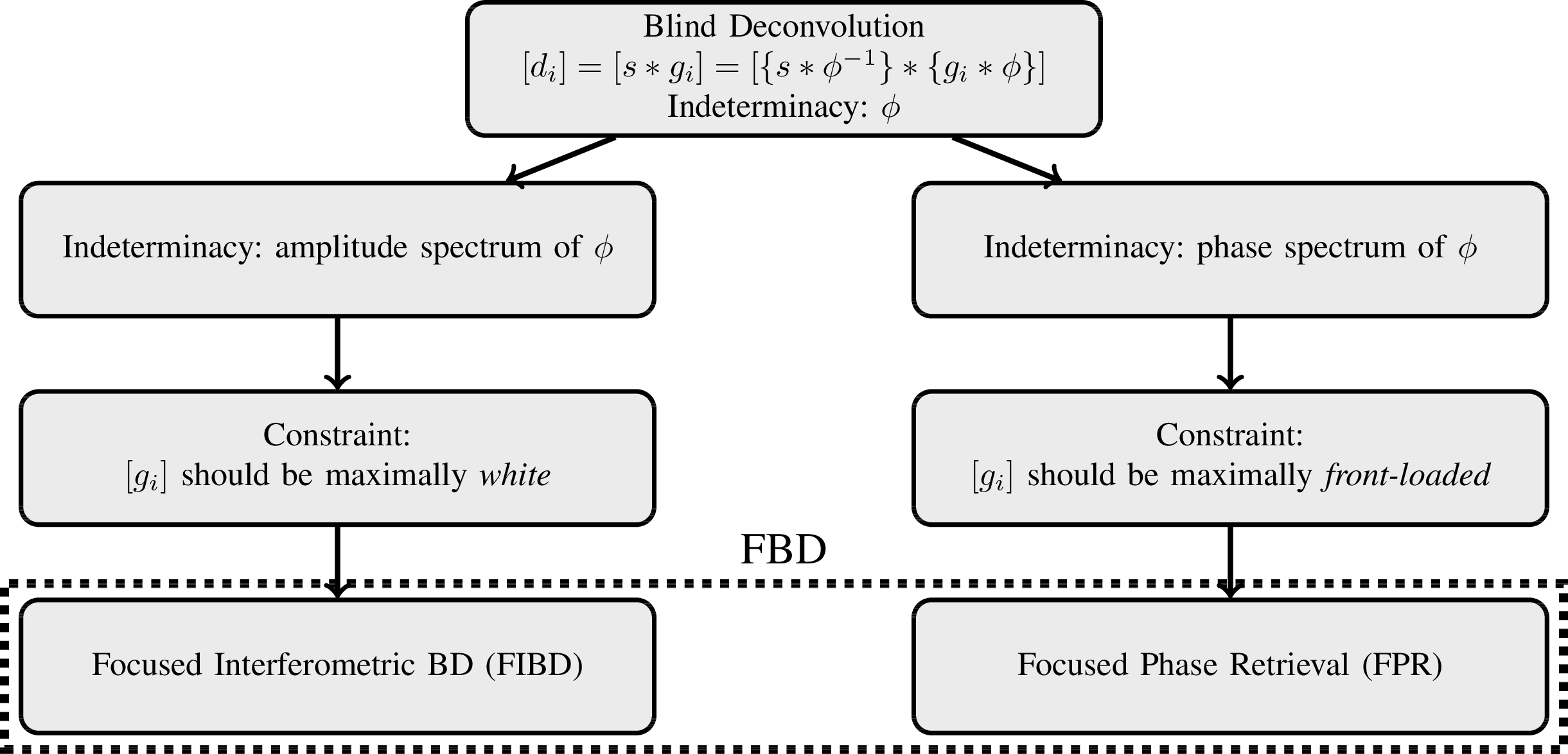
Figure 1: Focused blind deconvolution uses two focusing constraints to resolve the indeterminacies of the multichannel blind deconvolution. Note that this is not an algorithmic flowchart, but explains the two components of the regularization in FBD.

The aim of focused blind deconvolution is to seek the coprime solution of the LSBD problem. Otherwise, the channel polynomials $[\hat{G}_{i}]$ will typically be less sparse and less front-loaded in the time domain owing to the common roots that are associated with the undetermined filter $\phi$ of eq. 6. For example, including a common root $r$ to the polynomials in $[\hat{G}_{i}]$ implies an additional factor $(z-r)$ that corresponds to subtracting $[r\,g_{i}(t)]$ from $[g_{i}(t+1)]$ in the time domain, so that the sparsity is likely to reduce. Therefore, the intention and key innovation of FBD is to minimize the number of common roots in the channel polynomials $[\hat{G}_{i}]$ associated with $\Phi(z)$. It is difficult to achieve the same result with standard ideas from sparse regularization.

Towards this end, focused blind deconvolution solves a series of two least-squares optimization problems with focusing constraints. These constraints, described in the following subsections, can guide FBD to converge to the desired coprime solution. Note that this prescription does not guarantee that the recovered impulse responses should consistently match the true impulse responses; nevertheless, we empirically encounter a satisfactory recovery in most practical situations of seismic inversion, as discussed below.

The first problem considers fitting the cross-correlated channel outputs to jointly optimize two functions i.e., the impulse-response cross-correlations $[g_{ij}]$ between every possible channel pair and the source-signature auto-correlation ${{s}}_{\rm a}$. The focusing constraint in this problem will resolve the indeterminacy due to the amplitude spectrum of the unknown filter $\phi$ in eq. 6 such that the impulse responses $[g_{i}]$ are maximally white. Then the second problem completes the focused blind deconvolution by fitting the above-mentioned impulse-response cross-correlations, to estimate $[g_{i}]$ from $[g_{ij}]$. The focusing constraint in this problem will resolve the indeterminacy due to the phase spectrum of the unknown filter $\phi$ such that the impulse responses $[g_{i}]$ are maximally front-loaded. As shown in the Figure 1, these two problems will altogether resolve the indeterminacies of BD discussed in the previous section.

3.1 Focused Interferometric Blind Deconvolution

In order to isolate and resolve the indeterminacy due to the amplitude spectrum of $\phi(t)$, we consider a reformulated multichannel blind deconvolution problem. This reformulation deals with the cross-correlated or interferometric channel outputs, $d_{ij}:\{-T,\ldots,T\}\to\mathbb{R}$, as in eq. 2, between every possible channel pair (cf., Demanet and Jugnon,, 2017), therefore ending the indeterminacy due to the phase spectrum of $\phi(t)$.

Definition 2 (IBD: Interferometric Blind Deconvolution).

We use this problem to lay the groundwork for the next problem, and benchmarking. The optimization is carried out over the source-signature auto-correlation ${{s}}_{\rm a}:\{-T,\ldots,T\}\to\mathbb{R}$ and the cross-correlated or interferometric impulse responses $g_{ij}:\{-\tau,\ldots,\tau\}\to\mathbb{R}$:

$$V({{s}}_{\rm a},[g_{ij}]) =\sum_{k=1}^{\Nr}\sum_{l=k}^{\Nr}\sum_{t=-T}^{T}\{d_{kl}(t)-\{{{s}}_{\rm a}\ast g_{kl}\}(t)\}^{2}{;}$$ (7)

$$({\hat{s}}_{\rm a},[\hat{g}_{ij}]) =\mathop{\mathrm{arg\,min}}_{{{s}}_{\rm a},[g_{ij}]}\qquad V$$ (8)

$$\mathrm{subject\,\,to}\quad{{s}}_{\rm a}(0)=1;\quad{{s}}_{\rm a}(t)={{s}}_{\rm a}(-t){.}$$

Here, we denoted the $(\Nr+1)\Nr/2$-vector of unique interferometric impulse responses $[g_{11},g_{12},\ldots,g_{22},g_{23},\ldots,g_{\Nr\Nr}]$ by simply $[g_{ij}]$. We fit the interferometric outputs $d_{ij}$ after max normalization. The motivation of conveniently fixing ${{s}}_{\rm a}(0)$ is not only to resolve the scaling ambiguity but also to converge to a solution, where the necessary inequality condition ${{s}}_{\rm a}(t)\leq{{s}}_{\rm a}(0)\,\forall\,t$ is satisfied. More generally, the function ${{s}}_{\rm a}(t)$ is the autocorrelation of $s(t)$ if and only if the Toeplitz matrix formed from its translates is positive semidefinite, i.e., $\mbox{Toeplitz}({{s}}_{\rm a})\succeq 0$. This is a result known as Bochner’s theorem. This semidefinite constraint can be realized by projecting $\mbox{Toeplitz}({{s}}_{\rm a})$ onto the cone of positive semidefinite matrices at each iteration of the nonlinear least-squares iterative method (Vandenberghe and Boyd,, 1996). Nonetheless, in the numerical experiments, we observe convergence to acceptable solutions by just using the weaker constraints of IBD, when is data noise is sufficiently small.

Similar to LSBD, IBD has unwanted minimizers obtained by applying a filter $\psi^{-1}$ to ${{s}}_{\rm a}$ and $\psi$ to each element of $[g_{ij}]$, but it is easily computed that $\psi$ has to be real and nonnegative in the frequency domain ($|z|=1$) and related to the amplitude spectrum of $\phi(t)$. Therefore, its indeterminacy is lesser compared to that of the LSBD approach.

Definition 3 (FIBD: Focused Interferometric Blind Deconvolution).

FIBD starts by seeking a solution of the underdetermined IBD problem where the impulse responses are “maximally white", as measured by the concentration of their autocorrelation near zero lag. Towards that end, we use a regularizing term that penalizes the energy of the impulse-response auto-correlations proportional to the non-zero lag time $t$, before returning to solving the regular IBD problem.

$$W({{s}}_{\rm a},[g_{ij}]) =V({{s}}_{\rm a},[g_{ij}])+\alpha\sum_{k=1}^{\Nr}\sum_{t=-\tau}^{\tau}{t^{2}}g_{kk}^{2}(t){;}$$ (9)

$$({\hat{s}}_{\rm a},[\hat{g}_{ij}]) =\mathop{\mathrm{arg\,min}}_{{{s}}_{\rm a},[g_{ij}]}\qquad W$$ (10)

$$\mathrm{subject\,to}\quad{{s}}_{\rm a}(0)=1;\quad{{s}}_{\rm a}(t)={{s}}_{\rm a}(-t){.}$$

Here, $\alpha>0$ is a regularization parameter. We consider a homotopy (Osborne et al.,, 2000) approach to solve FIBD, where eq. 10 is solved in succession for decreasing values of $\alpha$, the result obtained for previous $\alpha$ being used as an initializer for the cycle that uses the current $\alpha$. The focusing constraint resolves the indeterminacy of IBD. Minimizing the energy of the impulse-response auto-correlations $[g_{ii}]$ proportional to the non-zero lag time will result in a solution where the impulse responses are heuristically as white as possible. In other words, FIBD minimizes the number of common roots, associated with the IBD indeterminacy $\Psi(z)$, in the estimated polynomials $[\hat{G}_{ij}]$, facilitating the goal of FBD to seek the coprime solution. The entire workflow of FIBD is shown in the Algorithm 1. In most of the numerical examples, we simply choose $\alpha=\infty$ first, and then $\alpha=0$.

3.2 Focused Phase Retrieval

FIBD resolves a component of the LSBD ambiguity and estimates the interferometric impulse responses. This should be followed by phase retrieval (PR) — a least-squares fitting of the interferometric impulse responses $[\hat{g}_{ij}]$ to optimize the impulse responses $[g_{i}]$. The estimation of $[g_{i}]$ in PR is hindered by the unresolved LSBD ambiguity due to the phase spectrum of $\phi(t)$. In order to resolve the remaining ambiguity, we use a focusing constraint in PR.

Definition 4 (LSPR: Least-squares Phase Retrieval).

Given the interferometric impulse responses $[g_{ij}]$, the aim of the phase retrieval problem is to estimate unknown $[g_{i}]$.

$$X([g_{i}]) =\sum_{k=1}^{\Nr}\sum_{l=i}^{\Nr}\sum_{t=-\tau}^{\tau}\{\hat{g}_{kl}(t)-\{g_{k}\otimes g_{l}\}(t)\}^{2}{;}$$ (11)

$$[\hat{g}_{i}] =\mathop{\mathrm{arg\,min}}_{[g_{i}]}\qquad X$$ (12)

LSPR is ill-posed. Consider a white filter $\chi(t)\neq\delta(t)$, where $\chi\otimes\chi=\delta$, that can be applied to each of the impulse responses, and leave their cross-correlations unchanged:

$$g_{ij}(t)=\{g_{i}\otimes g_{j}\}(t)=\{\{g_{i}\ast\chi\}\otimes\{g_{j}\ast\chi\}\}(t).$$ (13)

If furthermore $g_{i}\ast\chi$ obeys the constraint otherwise placed, namely in our case that the impulse responses should have duration length $\tau$, then we are in the presence of a true ambiguity not resolved by this constraint. It is obvious that the filter $\chi(t)$ is linked to the remaining unresolved component of the LSBD indeterminacy, i.e., the phase spectrum of $\phi(t)$.

Definition 5 (FPR: Focused Phase Retrieval).

FPR seeks a solution of the underdetermined LSPR problem where the impulse responses $[g_{i}]$ are “maximally front-loaded”. It starts with an optimization that fits the interferometric impulse responses only linked with the most front-loaded channel $f$, before returning to solving the regular LSPR problem. We use a regularizing term that penalizes the energy of the most front-loaded response $g_{f}$ proportional to the time $t\neq 0$:

$$Y([{g}_{i}]) =\sum_{k=1}^{\Nr}\sum_{t=-\tau}^{\tau}\{\hat{g}_{kf}(t)-\{g_{k}\otimes g_{f}\}(t)\}^{2}+\beta\,\sum_{t=0}^{\tau}g_{f}^{2}(t)t^{2};$$ (14)

$$[\hat{g}_{i}] =\mathop{\mathrm{arg\,min}}_{g_{i}}\qquad Y.$$ (15)

Here, $\beta\geq 0$ is a regularization parameter. Again, we consider a homotopy approach to solve this optimization problem, where the above equation is solved in succession for decreasing values of $\beta$. FPR chooses the undetermined filter $\chi$ such that $g_{i}\ast\chi$ has the energy maximally concentrated or focused at the front (small $t$). Minimizing the second moment of the squared impulse responses will result in a solution where the impulse responses are as front-loaded as possible. The entire workflow of FPR is shown in the Algorithm 2. In all the numerical examples, we simply choose $\beta=\infty$ first, and then $\beta=0$. Counting on the estimated impulse responses from FPR, we return to the LSBD formulation in order to finalize the BD problem.

3.3 Sufficiently Dissimilar Channel Configuration

FBD seeks the coprime solution of the ill-posed LSBD problem. Therefore, for the success of FBD, it is important that the true transfer functions do not share any common zeros in the $z$-domain. This requirement is satisfied when the channels are chosen to be sufficiently dissimilar. The channels are said to be sufficiently dissimilar unless there exists a spurious $\gamma$ and $[g_{i}]$ such that the true impulse-response vector $[g^{0}_{i}]=[\gamma\ast g_{i}]$. Here, $\gamma$ is a filter that 1. is independent of the channel index $i$; 2. belongs to the set $\mathbb{Q}$ of filters that cause indeterminacy of the LSBD problem; 3. doesn’t simply shift $g_{i}$ in time. In our experiments, FBD reconstructs a good approximation of the true impulse responses if the channels are sufficiently dissimilar. Otherwise, FBD outputs an undesirable solution $(s^{0}\ast\gamma^{-1},[g_{i}])$, as opposed to the desired $(s^{0},[\gamma\ast g_{i}])$, where $s^{0}$ is the true source signature. In the next section, we will show numerical examples with both similar and dissimilar channels.

• gg

generate the cross-correlated or interferometric channel outputs $[d_{ij}]$ and normalize with $d_{11}(0)$

gg

3 tolerance for convergence $\epsilon=10^{-8}$

$\vec{\alpha}=\set{\infty,0}$

gg

5 ${{s}}_{\rm a}(t)\leftarrow\begin{cases}0,&\text{if }t\neq 0\\ 1,&\text{otherwise}\end{cases}$

6 $g_{ij}(t)\leftarrow\begin{cases}0,&\text{if }i=j\,\text{and }t\neq 0\\ \operatorname{rand}(),&\text{otherwise}\end{cases}$

gg

8 interferometric transfer functions $[\hat{g}_{ij}]$

9 autocorrelation for the source signature $\hat{s}_{a}$ Kernel

10 foreach $\alpha\in{\vec{\alpha}}$ do /* loop over decreasing $\alpha$ */

11       $W_{1}=\infty$; $W_{2}=\infty$; $W_{1p}=W_{1}$; $W_{2p}=W_{2}$; $\Delta W=\infty$

12       while $\Delta W>\epsilon$ do

13            

14            ${s}_{a}\leftarrow\operatorname*{arg\,min}\limits_{s_{a}}W({{s}}_{\rm a},[{g}_{ij}])$ s.t. ${{s}}_{\rm a}(0)=1$ & ${{s}}_{\rm a}(t)={{s}}_{\rm a}(-t)$ /* updating source */

15             $W_{1p}\leftarrow W_{1}$; $W_{1}\leftarrow W({s}_{a},[{g}_{ij}])$

16             $[{g}_{ij}]\leftarrow\operatorname*{arg\,min}\limits_{[g_{ij}]}W({s}_{a},[g_{ij}])$

17             /* updating interferometric transfer functions */

18             $W_{2p}\leftarrow W_{2}$; $W_{2}\leftarrow W({s}_{a},[{g}_{ij}])$

19            

20            $\Delta W=\operatorname{max}(\set{W_{1p}-W_{1},W_{2p}-W_{2}}$) /* measure convergance */

21       end while

22      

23 end foreach

$[\hat{g}_{ij}]\leftarrow[g_{ij}$];  $\hat{s}_{a}\leftarrow s_{a}$

Algorithm 1 (Focused Interferometric Blind Deconvolution. Alternating minimization of $W$, as in eq. 10, is carried out in succession for decreasing values of $\alpha$.).

• gg

get the interferometric filters $[\hat{g}_{ij}]$ using FIBD

gg

3 $\vec{\beta}=\set{\infty,0}$

index of the most front-loaded channel $f$

gg

5 $g_{i}(t)\leftarrow\begin{cases}0,&\text{if }i=f\,\text{and }t\neq 0\\ \operatorname{rand}(),&\text{otherwise}\end{cases}$

gg

7 filters $[\hat{g}_{i}]$

8 Kernel

9 foreach $\beta\in{\vec{\beta}}$ do /* loop over decreasing $\beta$ */

10      

11      $[{g}_{i}]\leftarrow\operatorname*{arg\,min}\limits_{[g_{i}]}Y([{g}_{i}])$

12      

13 end foreach

14 $[{g}_{i}]\leftarrow\operatorname*{arg\,min}\limits_{[g_{i}]}X([g_{i}])$ /* return to LSPR */

$[\hat{g}_{i}]\leftarrow[g_{i}]$

Algorithm 2 (Focused Phase Retrieval. Solving $Y$, as in eq. 14, in succession for decreasing values of $\beta$. Then solving $X$ in eq. 11.).

4 Numerical Simulations

4.1 Idealized Experiment I

We consider an experiment with $\Nr=20$, $\tau=30$ and $T=400$. The aim is to reconstruct the true impulse responses $[g^{0}_{i}]$, plotted in Figure 2a, from the channel outputs generated using a Gaussian random source signature $s^{0}$. The impulse responses of similar kind are of particular interest in seismic inversion and room acoustics as they reveal the arrival of energy, propagated from an impulsive source, at the receivers in the medium. In this case, the arrivals have onsets of 6 s and 10 s at the first channel and they curve linearly and hyperbolically, respectively. The linear arrival is the earliest arrival that doesn’t undergo scattering. The hyperbolic arrival is likely to represent a wave that is reflected or scattered from an interface between two materials with different acoustic impedances.

LSBD

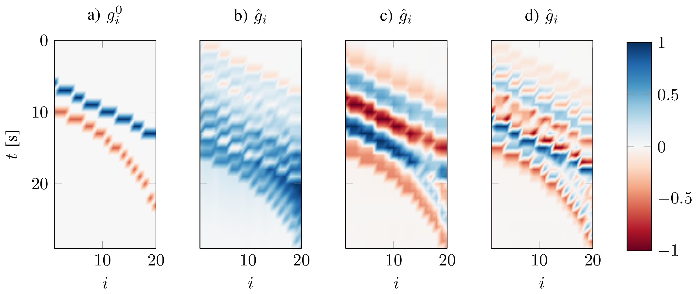
Figure 2: Idealized Experiment I. The results are displayed as images that use the full range of colors in a colormap. Each pixel of these images corresponds to a time $t$ and a channel index $i$. Impulse responses: a) true; b)—d) undesired.

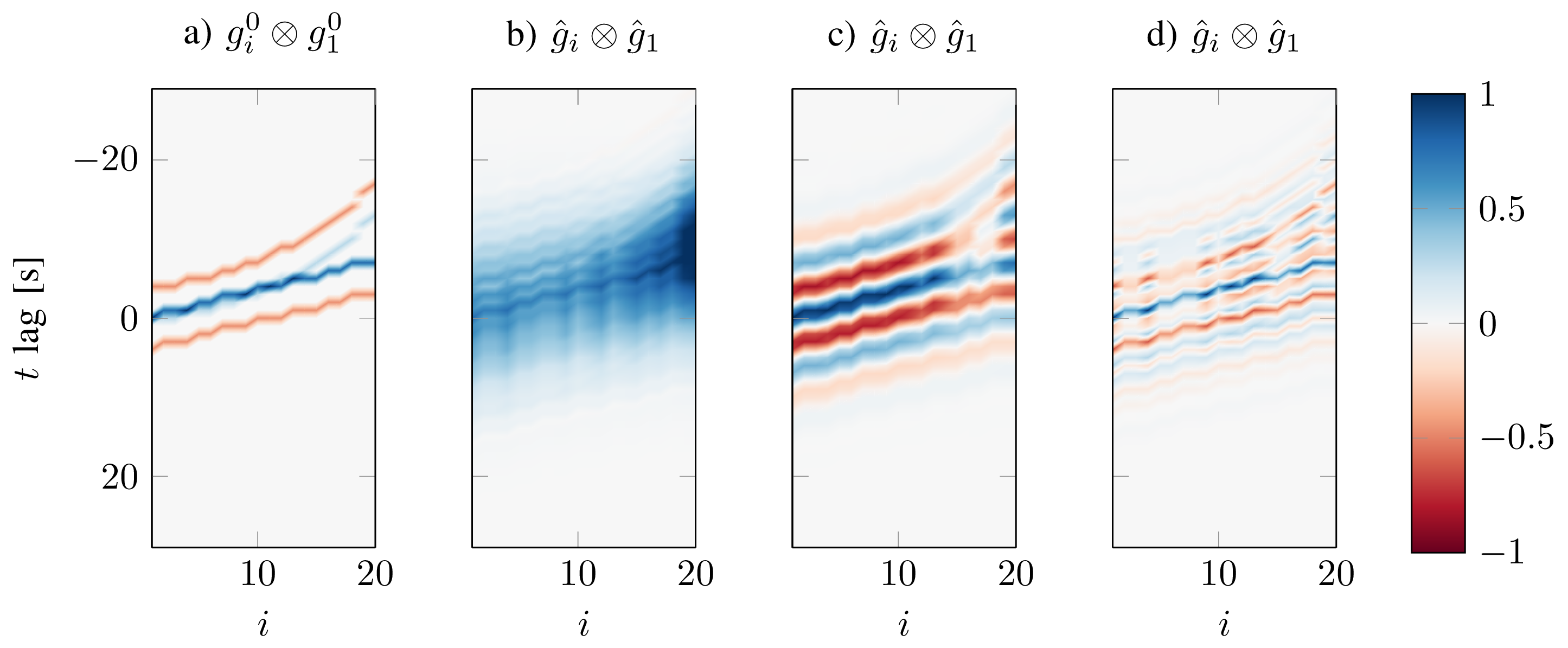
Figure 3: Idealized Experiment I. Cross-correlations of impulse responses corresponding to the Figure 2: a) true; b)—d) undesired.

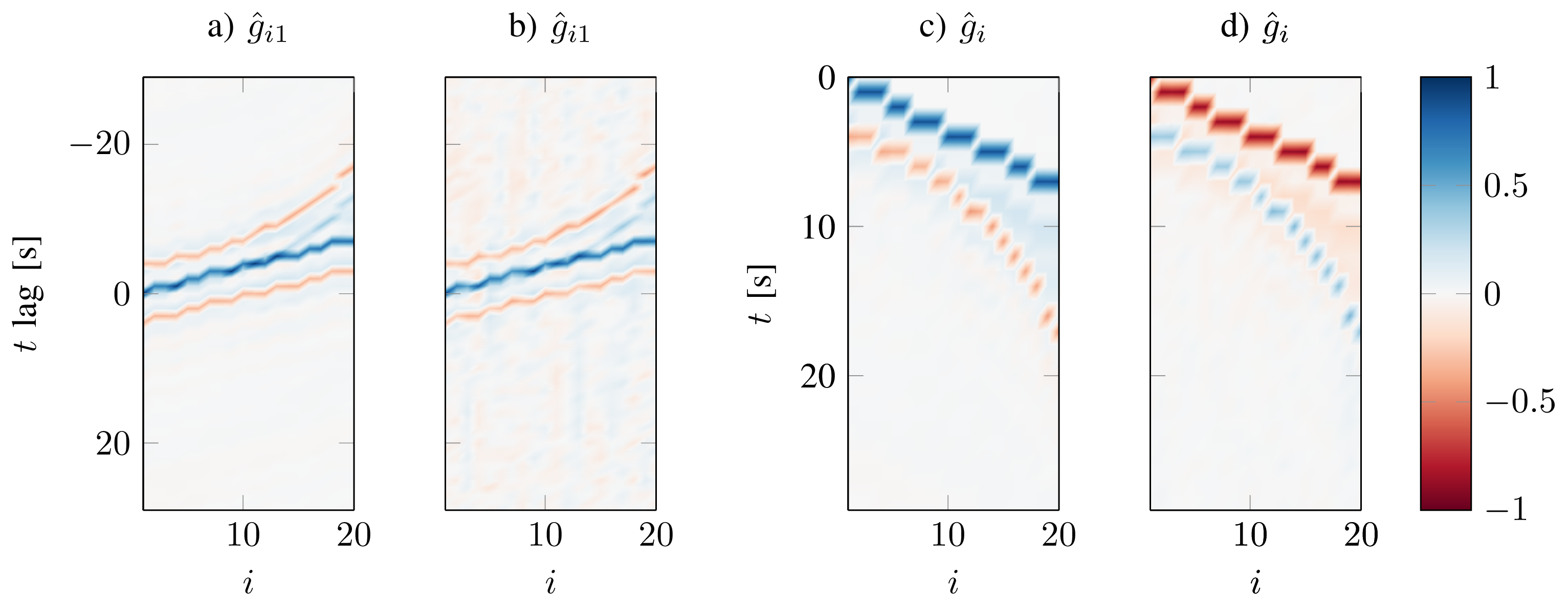
Figure 4: Idealized Experiment I. a) FIBD estimated interferometric impulse responses corresponding to the Figure 3a, after fitting the interferometric channel outputs. b) Same as (a), except after white noise is added to the channel outputs. c) Estimated impulse responses from FPR by fitting the FIBD-outcome interferometric impulse responses in (a). d) Same as (c), except fitting the FIBD outcome in (b).

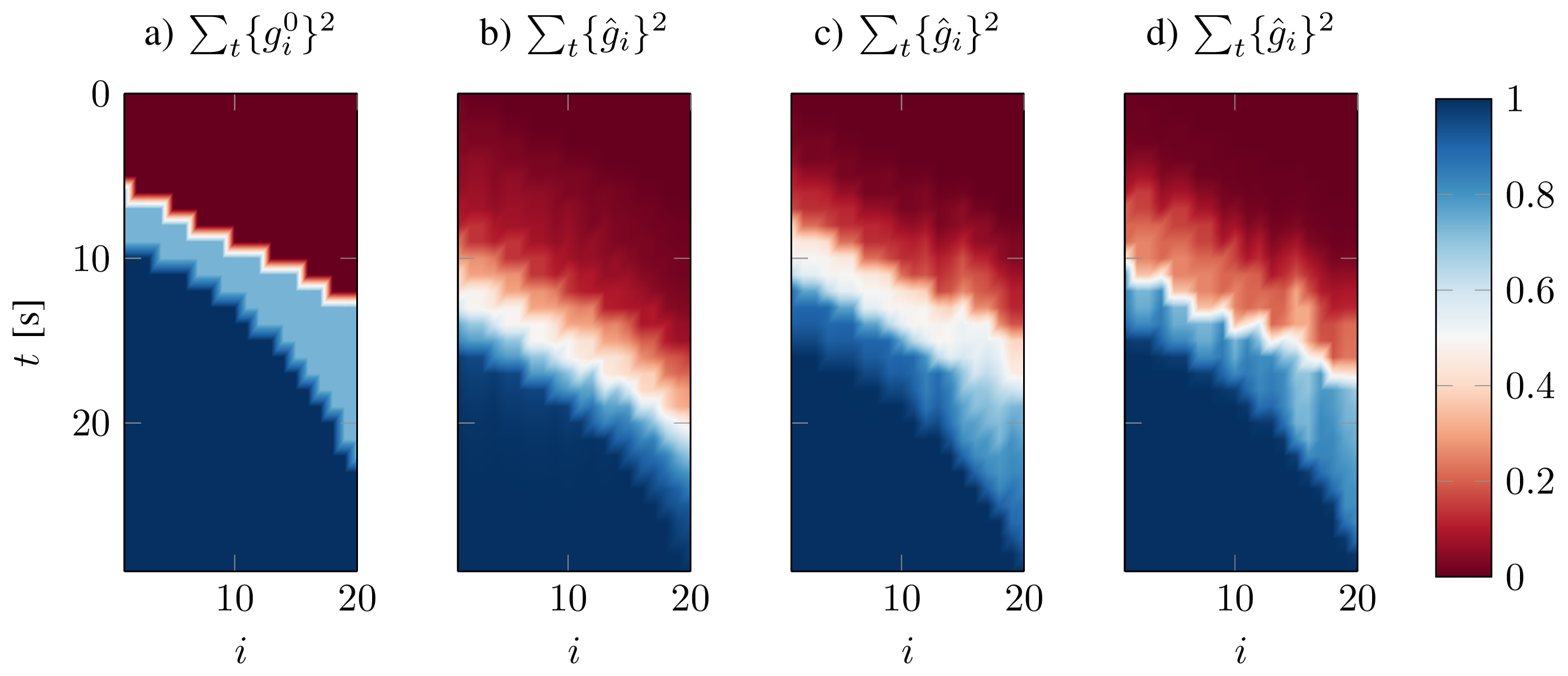
Figure 5: Idealized Experiment I. Normalized cumulative energy of: a) true; b)—d) undesired impulse responses corresponding to the Figure 2.

To illustrate its non-uniqueness, we use three different initial estimates of $s$ and $[g_{i}]$ to observe the convergence to three different solutions that belong to $\mathbb{P}$. The channel responses corresponding to these solutions are plotted in Figures 2b–d. At the convergence, the misfit (given in eq. 3) in all these three cases $U(\hat{s},[\hat{g}_{i}])\lessapprox 10^{-6}$, justifying non-uniqueness. Moreover, we notice that none of the solutions is desirable due to insufficient resolution.

FIBD

In order to isolate the indeterminacy due to the amplitude spectrum of the unknown filter $\phi(t)$ in eq. 6 and justify the use of the focusing constraint in eq. 9, we plot the true and undesirable impulse responses after cross-correlation in the Figure 3. It can be easily noticed that the true impulse-response cross-correlations corresponding to the first channel are more focused at $t=0$ than the undesirable impulse-response cross-correlations. The defocusing is caused by the ambiguity related to the amplitude spectrum of $\phi(t)$. FIBD in Algorithm 1 with $\vec{\alpha}=[\infty,0.0]$ resolves this ambiguity and satisfactorily recovers the true interferometric impulse responses $[g^{0}_{ij}]$, as plotted in Figure 4a. We regard the FIBD recovery be satisfactory in Figure 4b when the Gaussian white noise is added to the channel outputs so that the signal-to-noise (SNR) is $1\,$dB.

FPR

In order to motivate the use of the second focusing constraint, we plotted the normalized cumulative energy of the true and undesired impulse responses in the Figures 5. It can be easily noticed that the fastest rate of energy buildup in time occurs in the case of the true impulse responses. In other words, the energy of the true impulse responses is more front-loaded compared to undesired impulse responses, after neglecting an overall translation in time. The FPR in Algorithm 2 with $\vec{\beta}=[\infty,0]$ satisfactorily recovers $[g^{0}_{i}]$ that are plotted in: the Figure 4c — utilizing $[g_{ij}]$ recovered from the noiseless channel outputs (Figure 4a); the Figure 4d — utilizing $[g_{ij}]$ recovered from the channel outputs (Figure 4b) with Gaussian white noise. Note that the overall time translation and scaling cannot be fundamentally determined.

4.2 Idealized Experiment II

This IBD-benchmark experiment with $\Nr=20$ $\tau=30$ and $T=400$ aims to reconstruct simpler interferometric impulse responses, plotted in Figure 6b, corresponding to the true impulse responses in Figure 6a. A satisfactory recovery of $[g^{0}_{ij}]$ is not achievable without the focusing constraint — the IBD outcome in the Figure 6c doesn’t match the true interferometric impulse responses in the Figure 6b, unlike FIBD in the Figure 6d.

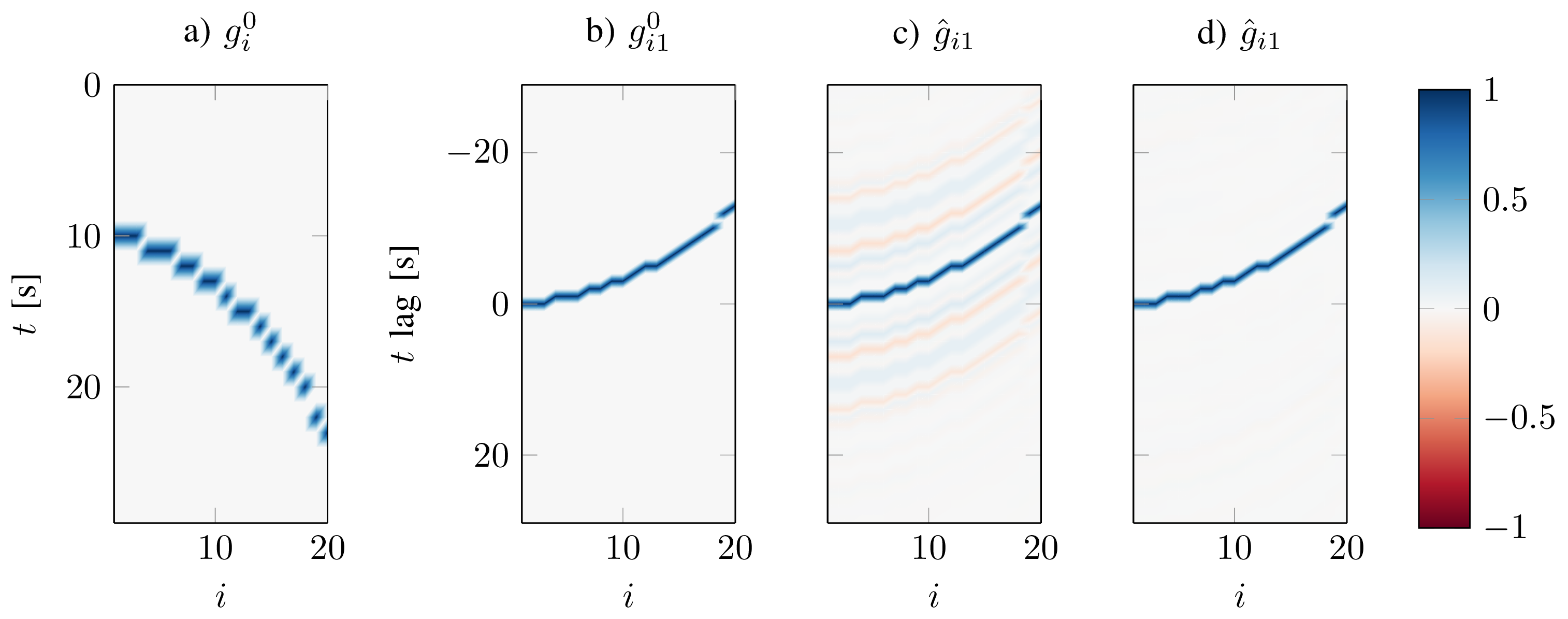
Figure 6: Idealized Experiment II. Interferometric impulse responses: a) true; b) estimated using IBD; c) estimated using FIBD.

4.3 Idealized Experiment III

We consider another experiment with $\Nr=20$ and $\tau=30$ to reconstruct the true impulse responses $[g^{0}_{i}]$ (plotted in Figure 7a) by fitting their cross-correlations $[g^{0}_{ij}]$. A satisfactory recovery of $[g^{0}_{i}]$ from $[g^{0}_{ij}]$ is not achievable without the focusing constraint — the outcome of LSPR, in Figure 7b, doesn’t match the true impulse responses, in Figure 7a, but is contaminated by the filter $\chi(t)$ in eq. 13. On the other hand, FPR results in the outcome (Figure 7c) that is not contaminated by $\chi(t)$.

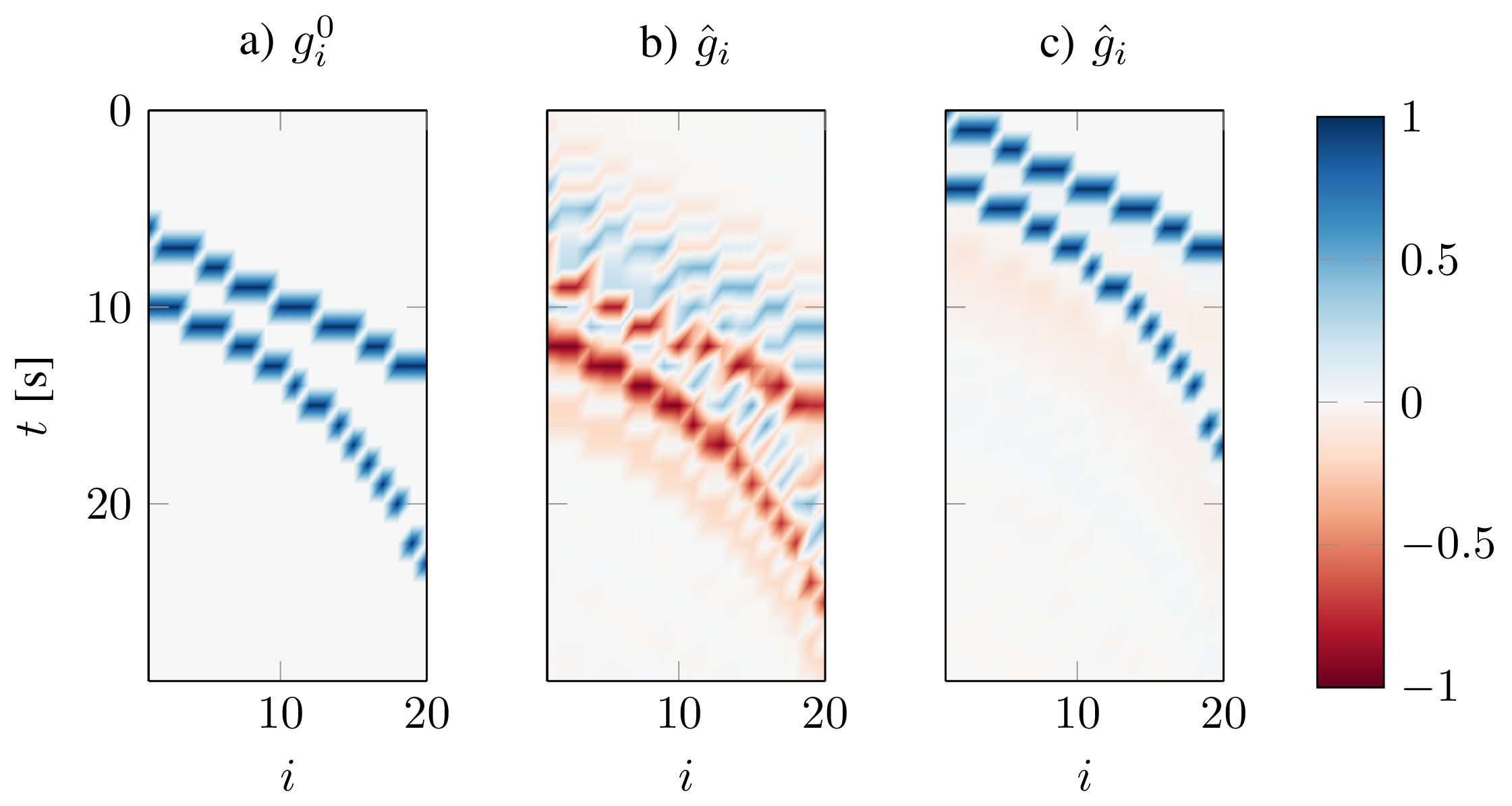
Figure 7: Idealized Experiment III. a) True impulse responses. b) Estimated impulse responses using LSPR. c) Estimated impulse responses using FPR.

4.4 Idealized Experiment IV

This experiment with $\Nr=20$, $\tau=30$ and $T=400$ aims to reconstruct the true interferometric impulse responses, plotted in Figure 8b, corresponding to the true impulse responses in Figure 8a. The outcome of FIBD with $\vec{\alpha}=[\infty,0]$, plotted in Figure 8c, doesn’t clearly match the true interferometric impulse responses because the channels are not sufficiently dissimilar. In this regard, observe that the Figure-8a true impulse responses at various channels $i$ differ only by a fixed time-translation instead of curving as in Figure 2a.

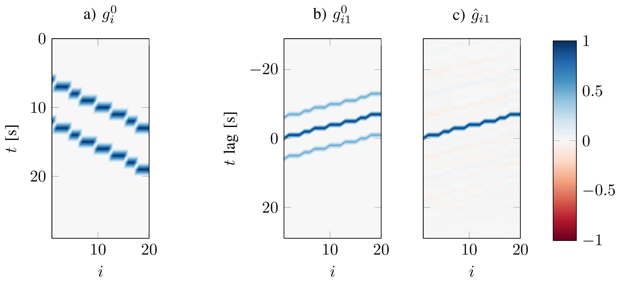
Figure 8: Idealized Experiment IV. a) True impulse responses of channels that are not sufficiently dissimilar. b) True interferometric impulse responses corresponding to (a). c) FIBD estimated interferometric impulse responses corresponding to (b), after fitting the interferometric channel outputs.

4.5 Idealized Experiment V

We consider another experiment with $\Nr=20$ and $\tau=30$ to reconstruct the true impulse responses $[g^{0}_{i}]$ (plotted in Figure 9a) that are not front-loaded, by fitting their cross-correlations $[g^{0}_{ij}]$. The FPR estimated impulse responses $[\hat{g}_{i}]$, plotted in Figure 9b, do not clearly depict the arrivals because there exists a spurious $\chi\neq\delta$ obeying eq. 13, such that $[g^{0}_{i}\ast\chi]$ are more front-loaded than $[g^{0}_{i}]$. We observe that FPR typically doesn’t result in a favorable outcome if the impulse responses are not front-loaded. Otherwise, the front-loaded $[g^{0}_{i}]$, plotted in Figure 9c, are successfully reconstructed in Figure 9d, except for an overall translation in time.

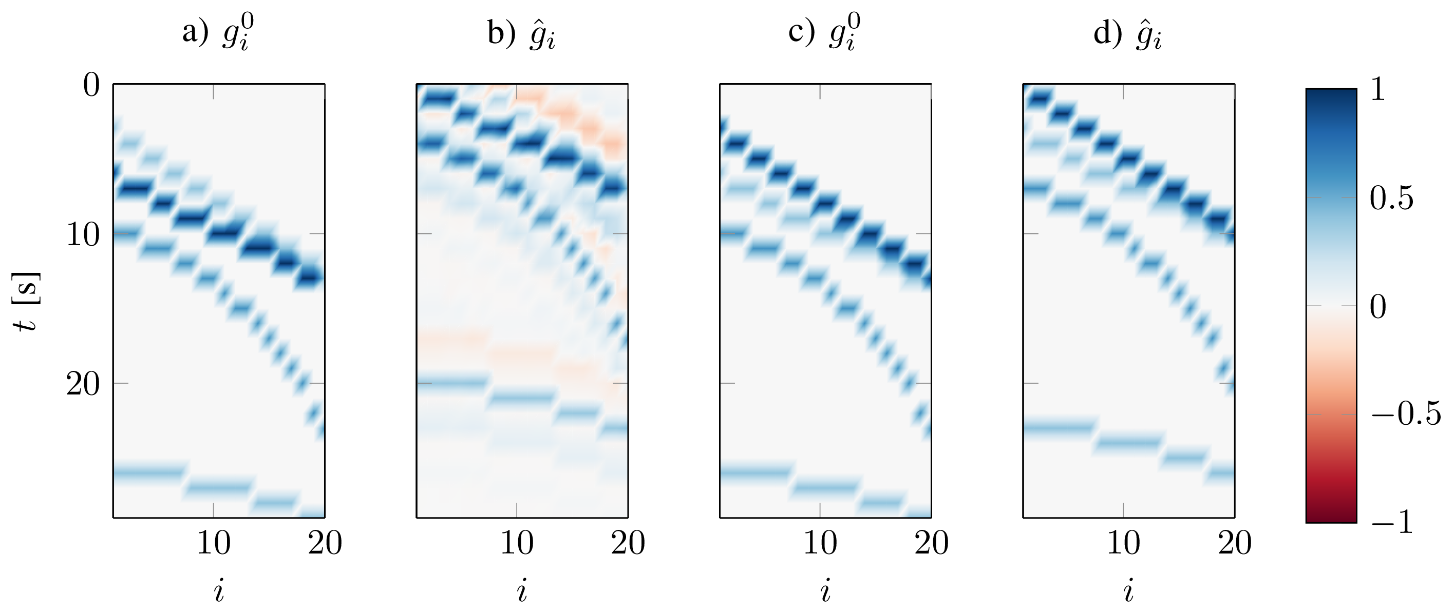
Figure 9: Idealized Experiment V. a) True impulse responses that are not front-loaded. b) FPR estimated impulse responses corresponding to (a), after fitting the true interferometric impulse responses. c) Same as (a), but front-loaded. d) Same as (b), but corresponding to (c).

5 Green’s function Retrieval

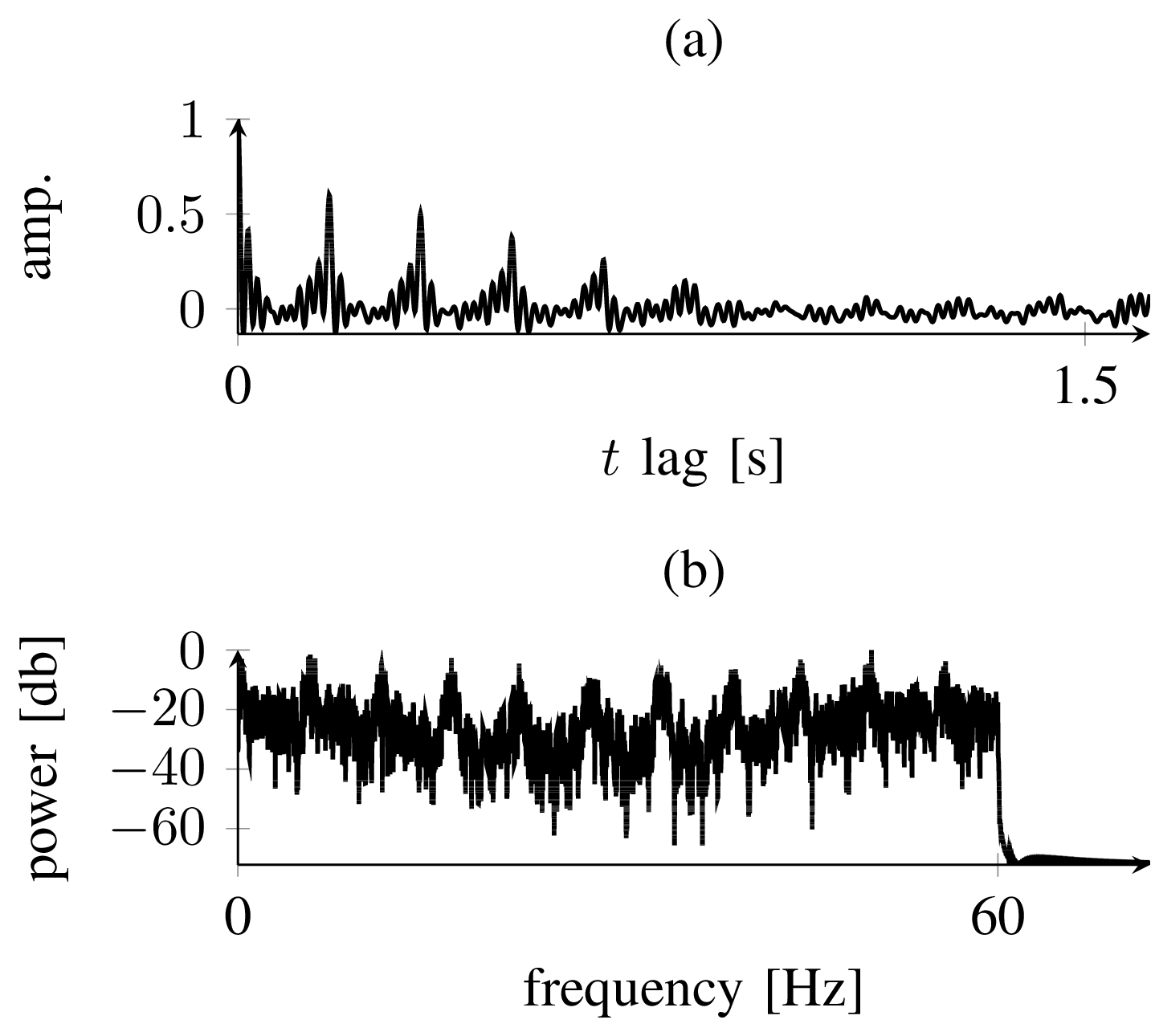
Figure 10: Source signature for the seismic experiment. (a) auto-correlation that contaminates the interferometric Green’s functions in the time domain — only 5% of $T$ is plotted; (b) power spectrum, where the Nyquist frequency is $60\,$Hz.

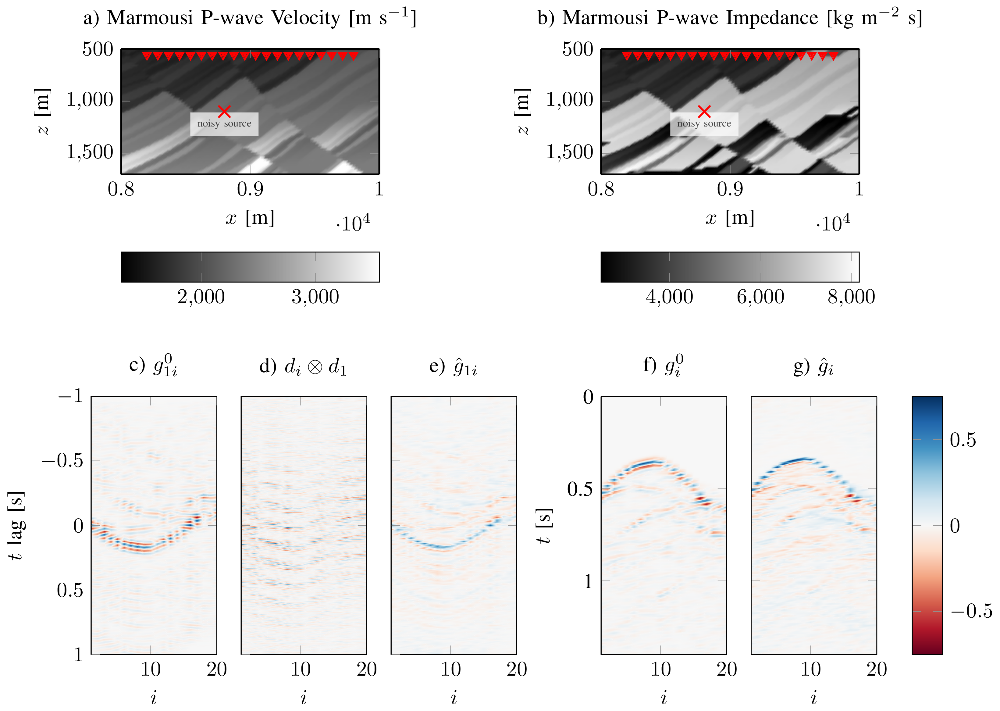
Figure 11: Seismic Experiment. a) Acoustic velocity model for wave propagation. b) Acoustic impedance model depicting interfaces that reflect waves. c) True interferometric Green’s functions. d) Seismic interferometry by cross-correlation. e) FIBD estimated interferometric Green’s functions. f) True Green’s functions. g) FBD estimated Green’s functions.

Finally, we consider a more realistic scenario involving seismic-wave propagation in a complex 2-D structural model, which is commonly known as the Marmousi model (Brougois et al.,, 1990) in exploration seismology. The Marmousi P-wave velocity and impedance plots are in the Figures 11a and 11b, respectively. We inject an unknown band-limited source signal, e.g., due to a drill bit, into this model for $30\,$s, such that $T=3600$. The signal’s auto-correlation and power spectrum are plotted in Figures 10a and 10b, respectively. We used an acoustic time-domain staggered-grid finite-difference solver for wave-equation modeling. The recorded seismic data at twenty receivers spaced roughly $100\,$m apart, placed at a depth of roughly $500\,$m, can be modeled as the output of a linear system that convolves the source signature with the Earth’s impulse response, i.e., its Green’s function. We recall that in the seismic context:

• the impulse responses $[g_{i}]$ correspond to the unique subsurface Green’s function $g(\vec{x},t)$ evaluated at the receiver locations $[\vec{x}_{i}]$, where the seismic-source signals are recorded;

• the channel outputs $[d_{i}]$ correspond to the noisy subsurface wavefield $d(\vec{x},t)$ recorded at the receivers only for $\{0,\ldots,T\}$ — we are assuming that the source may be arbitrarily on or off throughout this time interval, just as in usual drilling operations;

• $\tau$ denotes the propagation time necessary for the seismic energy, including multiple scattering, traveling from the source to a total of $\Nr$ receivers, to decrease below an ad-hoc threshold.

The goal of this experiment is to reconstruct the subsurface Green’s function vector $[g_{i}]$ that contains: 1. the direct arrival from the source to the receivers and 2. the scattered waves from various interfaces in the model. The ‘true’ Green’s functions $g^{0}_{i}$ and the interferometric Green’s functions $g^{0}_{ij}$, in Figures 11f and 11c, are generated following these steps: 1. get data for $1.5\,$s ($\tau=180$) using a Ricker source wavelet (basically a degree-2 Hermite function modulated to a peak frequency of 20 Hz); 2. create cross-correlated data necessary for $[g^{0}_{ij}]$; and 3. perform a deterministic deconvolution on the data using the Ricker wavelet. Observe that we have chosen the propagation time to be $1.5\,$s, such that $T/\tau=20$.

Seismic interferometry by cross-correlation (see eq. 2) fails to retrieve direct and the scattered arrivals in the true interferometric Green’s functions, as the cross-correlated data $[d_{ij}]$, plotted in Figure 11d, is contaminated by the auto-correlation of the source signature (Figure 10a). Therefore, we use FBD to first extract the interferometric Green’s functions by FIBD, plotted in the Figure 11e, and then recover the Green’s functions, plotted in the Figure 11g, using FPR. Notice that the FBD estimated Green’s functions clearly depict the direct and the scattered arrivals, confirming that our method doesn’t suffer from the complexities in the subsurface models.

6 Conclusions

Focused blind deconvolution (FBD) solves a series of two optimization problems in order to perform multichannel blind deconvolution (BD), where both the unknown impulse responses and the unknown source signature are estimated given the channel outputs. It is designed for a BD problem where the impulse responses are supposed to be sparse, front-loaded and shorter in duration compared to the channel outputs; as in the case of seismic inversion with a noisy source. The optimization problems use focusing constraints to resolve the indeterminacy inherent to the traditional BD. The first problem considers fitting the interferometric channel outputs and focuses the energy of the impulse-response auto-correlations at the zero lag to estimate the interferometric impulse responses and the source auto-correlation. The second problem completes FBD by fitting the estimated interferometric impulse responses, while focusing the energy of the most front-loaded channel at the zero time. FBD doesn’t require any support constraints on the unknowns. We have demonstrated the benefits of FBD using seismic experiments.

7 Acknowledgements

The material is based upon work assisted by a grant from Equinor. Any opinions, findings, and conclusions or recommendations expressed in this material are those of the authors and do not necessarily reflect the views of Equinor. The authors thank Ali Ahmed, Antoine Paris, Dmitry Batenkov and Matt Li from MIT for helpful discussions, and Ioan Alexandru Merciu from Equinor for his informative review and commentary of a draft version. LD is also supported by AFOSR grant FA9550-17-1-0316, and NSF grant DMS-1255203.

Appendix A Appendix

In this appendix, we present a simple justification of the ability of a focusing functional on the autocorrelation to select for sparsity, in a setting where $\ell_{1}$ minimization is unable to do so. This setting is the special case of a vector with nonnegative entries, made less sparse by convolution with another vector with nonnegative entries as well. This scenario is not fully representative of the more general formulation assumed in this paper, where cancelations may occur because of alternating signs. It seems necessary, however, to make an assumption of no cancelation (like positivity) in order to obtain the type of comparison result that we show in this section.

Consider two infinite sequences $f_{i}$ and $\phi_{j}$, for $i,j\in\mathbb{Z}$ (the set of integers), with sufficient decay so that all the expressions below make sense, and all the sum swaps are valid. Assume that $f_{i}\geq 0$ and $\phi_{i}\geq 0$ for all $i\in\mathbb{Z}$, not identically zero. Let

$$g_{j}=(f*\phi)_{j}=\sum_{i\in\mathbb{Z}}f_{i}\phi_{j-i},$$

which obviously also obeys $g_{i}\geq 0$ for all $i\in Z$. Assume the normalization condition $\sum_{i\in\mathbb{Z}}\phi_{i}=1$.

Now consider the autocorrelations

$$F_{j}=(f\otimes f)_{j}=\sum_{i}f_{i}f_{j+i},\qquad G_{j}=(g\otimes g)_{j}=\sum_{i}g_{i}g_{j+i},$$

and a specific choice of focusing functional,

$$J_{F}=\sum_{j\in Z}j^{2}F_{j},\qquad J_{G}=\sum_{j\in\mathbb{Z}}j^{2}G_{j}.$$

Proposition 1.

$$J_{G}\geq J_{F},$$

with equality if and only if $\phi_{i}$ is the Kronecker $\delta_{i0}$.

Proof.

All sums run over $\mathbb{Z}$. Start by observing

$$J_{F}=\sum_{j}\sum_{k}K_{jk}f_{j}f_{k},\qquad K_{jk}=(j-k)^{2},$$

and

$$J_{G}=\sum_{j}\sum_{k}L_{jk}f_{j}f_{k},\qquad L_{jk}=\sum_{m}\sum_{n}\left((j-k)-(m-n)\right)^{2}\phi_{m}\phi_{n}.$$

For any particular value $m-n=a$, we have

$$\sum_{j}\sum_{k}\left((j-k)-a\right)^{2}f_{j}f_{k} =a^{2}\sum_{j}\sum_{k}f_{j}f_{k}+\sum_{j}\sum_{k}(j-k)^{2}f_{j}f_{k}$$

$$\geq J_{F},$$

(the term linear in $j-k$ drops because $j-k$ is antisymmetric in $j$ and $k$, while $f_{j}f_{k}$ is symmetric), with equality if and only if $a=0$.

Now $J_{G}$ is a convex combination of such contributions:

$$\sum_{m}\sum_{n}\left[\sum_{j}\sum_{k}\left((j-k)-(m-n)\right)^{2}f_{j}f_{k}\right]\phi_{m}\phi_{n} \geq\sum_{m}\sum_{n}\left[J_{F}\right]\phi_{m}\phi_{n}$$

$$=J_{F}$$

with equality if and only if the cartesian product supp $\phi\;\times$ supp $\phi$ contains only the diagonal $m=n$. This latter scenario only arises when supp $\phi=\{0\}$, which is only compatible with $\sum_{i}\phi_{i}=1$ when $\phi_{i}=\delta_{i0}$. ∎

In contrast, notice that $\sum_{i}f_{i}=\sum_{i}g_{i}$, hence $f$ and $g$ cannot be discriminated with the $\ell_{1}$ norm. The $\ell_{1}$ norm is unable to measure the extent to which the support of $f$ was “spread" by convolution with $\phi$, when $\sum\phi_{i}=1$, and when all the functions are nonnegative.

The continuous counterpart of this result, for nonnegative functions $f(t)$ and $g(t)=\int f(s)\phi(t-s)ds$, with nonnegative $\phi$ such that $\int\phi(t)dt=1$ in the sense of measures, involves the autocorrelations

$$F(t)=(f\otimes f)(t)=\int f(s)f(s+t)ds,\qquad G(t)=(g\otimes g)(t),$$

and focusing functionals

$$J_{F}=\int t^{2}F(t)dt,\qquad J_{G}=\int t^{2}G(t)dt.$$

Then, $J_{G}\geq J_{F}$, with equality if and only if $\phi(t)=\delta(t)$, the Dirac delta.

References

- Ahmed et al., (2015) Ahmed, A., A. Cosse, and L. Demanet, 2015, A convex approach to blind deconvolution with diverse inputs: Computational Advances in Multi-Sensor Adaptive Processing (CAMSAP), 2015 IEEE 6th International Workshop on, IEEE, 5–8.
- Ahmed and Demanet, (2016) Ahmed, A., and L. Demanet, 2016, Leveraging diversity and sparsity in blind deconvolution: arXiv preprint arXiv:1610.06098.
- Amari et al., (1997) Amari, S.-i., S. C. Douglas, A. Cichocki, and H. H. Yang, 1997, Multichannel blind deconvolution and equalization using the natural gradient: Signal Processing Advances in Wireless Communications, First IEEE Signal Processing Workshop on, IEEE, 101–104.
- Aminzadeh and Dasgupta, (2013) Aminzadeh, F., and S. N. Dasgupta, 2013, Geophysics for petroleum engineers: Newnes, 60.
- Ayers and Dainty, (1988) Ayers, G., and J. C. Dainty, 1988, Iterative blind deconvolution method and its applications: Optics letters, 13, 547–549.
- Bharadwaj et al., (2017) Bharadwaj, P., L. Demanet, and A. Fournier, 2017, Deblending random seismic sources via independent component analysis: Presented at the SEG Technical Program Expanded Abstracts, Society of Exploration Geophysicists.
- Bharadwaj et al., (2018) ——–, 2018, Focused blind deconvolution of interferometric Green’s functions: Presented at the SEG Technical Program Expanded Abstracts, Society of Exploration Geophysicists.
- Borcea et al., (2006) Borcea, L., G. Papanicolaou, and C. Tsogka, 2006, Coherent interferometric imaging in clutter: Geophysics, 71, SI165–SI175.
- Broggini et al., (2014) Broggini, F., R. Snieder, and K. Wapenaar, 2014, Data-driven wavefield focusing and imaging with multidimensional deconvolution: Numerical examples for reflection data with internal multiples: Geophysics, 79, WA107–WA115.
- Brougois et al., (1990) Brougois, A., M. Bourget, P. Lailly, M. Poulet, P. Ricarte, and R. Versteeg, 1990, Marmousi, model and data: Presented at the EAEG Workshop-Practical Aspects of Seismic Data Inversion.
- Campisi and Egiazarian, (2016) Campisi, P., and K. Egiazarian, 2016, Blind image deconvolution: theory and applications: CRC press.
- Claerbout, (1968) Claerbout, J. F., 1968, Synthesis of a layered medium from its acoustic transmission response: Geophysics, 33, 264–269.
- Curtis et al., (2006) Curtis, A., P. Gerstoft, H. Sato, R. Snieder, and K. Wapenaar, 2006, Seismic interferometry—turning noise into signal: The Leading Edge, 25, 1082–1092.
- Demanet and Jugnon, (2017) Demanet, L., and V. Jugnon, 2017, Convex recovery from interferometric measurements: IEEE Transactions on Computational Imaging, 3, 282–295.
- Douglas et al., (1997) Douglas, S. C., A. Cichocki, and S.-I. Amari, 1997, Multichannel blind separation and deconvolution of sources with arbitrary distributions: Neural Networks for Signal Processing [1997] VII. Proceedings of the 1997 IEEE Workshop, IEEE, 436–445.
- Draganov et al., (2006) Draganov, D., K. Wapenaar, and J. Thorbecke, 2006, Seismic interferometry: Reconstructing the earth’s reflection response: Geophysics, 71, SI61–SI70.
- Gaubitch et al., (2005) Gaubitch, N. D., J. Benesty, and P. A. Naylor, 2005, Adaptive common root estimation and the common zeros problem in blind channel identification: Signal Processing Conference, 2005 13th European, IEEE, 1–4.
- Gradl et al., (2012) Gradl, C., A. W. Eustes, and G. Thonhauser, 2012, An analysis of noise characteristics of drill bits: Journal of energy resources technology, 134, 013103.
- Haldorsen et al., (1995) Haldorsen, J. B., D. E. Miller, and J. J. Walsh, 1995, Walk-away vsp using drill noise as a source: Geophysics, 60, 978–997.
- Huang and Benesty, (2002) Huang, Y. A., and J. Benesty, 2002, Adaptive multi-channel least mean square and newton algorithms for blind channel identification: Signal Processing, 82, 1127–1138.
- Joyce et al., (2001) Joyce, B., D. Patterson, J. Leggett, and V. Dubinsky, 2001, Introduction of a new omni-directional acoustic system for improved real-time LWD sonic logging-tool design and field test results: Presented at the SPWLA 42nd Annual Logging Symposium, Society of Petrophysicists and Well-Log Analysts.
- Kaaresen and Taxt, (1998) Kaaresen, K. F., and T. Taxt, 1998, Multichannel blind deconvolution of seismic signals: Geophysics, 63, 2093–2107.
- Kazemi et al., (2016) Kazemi, N., E. Bongajum, and M. D. Sacchi, 2016, Surface-consistent sparse multichannel blind deconvolution of seismic signals: IEEE Transactions on geoscience and remote sensing, 54, 3200–3207.
- Kazemi and Sacchi, (2014) Kazemi, N., and M. D. Sacchi, 2014, Sparse multichannel blind deconvolution: Geophysics, 79, V143–V152.
- Khong et al., (2008) Khong, A. W., X. Lin, and P. A. Naylor, 2008, Algorithms for identifying clusters of near-common zeros in multichannel blind system identification and equalization: Acoustics, Speech and Signal Processing, 2008. ICASSP 2008. IEEE International Conference on, IEEE, 389–392.
- Kundur and Hatzinakos, (1996) Kundur, D., and D. Hatzinakos, 1996, Blind image deconvolution: IEEE signal processing magazine, 13, 43–64.
- Li et al., (2016) Li, X., S. Ling, T. Strohmer, and K. Wei, 2016, Rapid, robust, and reliable blind deconvolution via nonconvex optimization: arXiv preprint arXiv:1606.04933.
- Liu et al., (2016) Liu, E., N. Iqbal, J. H. McClellan, and A. A. Al-Shuhail, 2016, Sparse blind deconvolution of seismic data via spectral projected-gradient: arXiv preprint arXiv:1611.03754.
- Liu and Malvar, (2001) Liu, J., and H. Malvar, 2001, Blind deconvolution of reverberated speech signals via regularization: Acoustics, Speech, and Signal Processing, 2001. Proceedings.(ICASSP’01). 2001 IEEE International Conference on, IEEE, 3037–3040.
- Liu and Liu, (2003) Liu, X., and H. Liu, 2003, Survey on seismic blind deconvolution: Progress in Geophysics, 18, 203–209.
- Makino et al., (2005) Makino, S., H. Sawada, R. Mukai, and S. Araki, 2005, Blind source separation of convolutive mixtures of speech in frequency domain: IEICE Transactions on Fundamentals of Electronics, Communications and Computer Sciences, 88, 1640–1655.
- Nose-Filho et al., (2015) Nose-Filho, K., A. K. Takahata, R. Lopes, and J. M. Romano, 2015, A fast algorithm for sparse multichannel blind deconvolution: Geophysics, 81, V7–V16.
- Osborne et al., (2000) Osborne, M. R., B. Presnell, and B. A. Turlach, 2000, A new approach to variable selection in least squares problems: IMA journal of numerical analysis, 20, 389–403.
- Rector III and Marion, (1991) Rector III, J., and B. P. Marion, 1991, The use of drill-bit energy as a downhole seismic source: Geophysics, 56, 628–634.
- Robinson, (1957) Robinson, E. A., 1957, Predictive decomposition of seismic traces: Geophysics, 22, 767–778.
- Robinson and Treitel, (1980) Robinson, E. A., and S. Treitel, 1980, Geophysical signal analysis: Prentice-Hall Englewood Cliffs, NJ, 263.
- Romberg et al., (2013) Romberg, J., N. Tian, and K. Sabra, 2013, Multichannel blind deconvolution using low rank recovery: Independent Component Analyses, Compressive Sampling, Wavelets, Neural Net, Biosystems, and Nanoengineering XI, International Society for Optics and Photonics, 87500E.
- Schuster et al., (2004) Schuster, G., J. Yu, J. Sheng, and J. Rickett, 2004, Interferometric/daylight seismic imaging: Geophysical Journal International, 157, 838–852.
- Schuster, (2009) Schuster, G. T., 2009, Seismic interferometry: Cambridge University Press Cambridge, 1.
- Shapiro et al., (2005) Shapiro, N. M., M. Campillo, L. Stehly, and M. H. Ritzwoller, 2005, High-resolution surface-wave tomography from ambient seismic noise: Science, 307, 1615–1618.
- Snieder, (2004) Snieder, R., 2004, Extracting the green’s function from the correlation of coda waves: A derivation based on stationary phase: Physical Review E, 69, 046610.
- Snieder and Safak, (2006) Snieder, R., and E. Safak, 2006, Extracting the building response using seismic interferometry: Theory and application to the millikan library in pasadena, california: Bulletin of the Seismological Society of America, 96, 586–598.
- Sroubek and Flusser, (2003) Sroubek, F., and J. Flusser, 2003, Multichannel blind iterative image restoration: IEEE Transactions on Image Processing, 12, 1094–1106.
- Sroubek and Milanfar, (2012) Sroubek, F., and P. Milanfar, 2012, Robust multichannel blind deconvolution via fast alternating minimization: IEEE Transactions on Image Processing, 21, 1687–1700.
- Subramaniam et al., (1996) Subramaniam, S., A. P. Petropulu, and C. Wendt, 1996, Cepstrum-based deconvolution for speech dereverberation: IEEE transactions on speech and audio processing, 4, 392–396.
- Tong and Perreau, (1998) Tong, L., and S. Perreau, 1998, Multichannel blind identification: From subspace to maximum likelihood methods: Proceedings of the IEEE, 86, 1951–1968.
- Tong et al., (1995) Tong, L., G. Xu, B. Hassibi, and T. Kailath, 1995, Blind channel identification based on second-order statistics: A frequency-domain approach: IEEE Transactions on Information Theory, 41, 329–334.
- Tong et al., (1994) Tong, L., G. Xu, and T. Kailath, 1994, Blind identification and equalization based on second-order statistics: A time domain approach: IEEE Transactions on information Theory, 40, 340–349.
- Ulrych et al., (1995) Ulrych, T. J., D. R. Velis, and M. D. Sacchi, 1995, Wavelet estimation revisited: The Leading Edge, 14, 1139–1143.
- Van der Baan and Pham, (2008) Van der Baan, M., and D.-T. Pham, 2008, Robust wavelet estimation and blind deconvolution of noisy surface seismics: Geophysics.
- van der Neut et al., (2011) van der Neut, J., J. Thorbecke, K. Mehta, E. Slob, and K. Wapenaar, 2011, Controlled-source interferometric redatuming by crosscorrelation and multidimensional deconvolution in elastic media: Geophysics, 76, SA63–SA76.
- Vandenberghe and Boyd, (1996) Vandenberghe, L., and S. Boyd, 1996, Semidefinite programming: SIAM review, 38, 49–95.
- Vasconcelos and Snieder, (2008) Vasconcelos, I., and R. Snieder, 2008, Interferometry by deconvolution: Part 1—theory for acoustic waves and numerical examples: Geophysics, 73, S115–S128.
- Vidal et al., (2014) Vidal, C. A., D. Draganov, J. Van der Neut, G. Drijkoningen, and K. Wapenaar, 2014, Retrieval of reflections from ambient noise using illumination diagnosis: Geophysical Journal International, 198, 1572–1584.
- Wapenaar and Fokkema, (2006) Wapenaar, K., and J. Fokkema, 2006, Green’s function representations for seismic interferometry: Geophysics, 71, SI33–SI46.
- Wapenaar et al., (2006) Wapenaar, K., E. Slob, and R. Snieder, 2006, Unified green’s function retrieval by cross correlation: Physical Review Letters, 97, 234301.
- Wapenaar et al., (2008) Wapenaar, K., J. van der Neut, and E. Ruigrok, 2008, Passive seismic interferometry by multidimensional deconvolution: Geophysics, 73, A51–A56.
- Wapenaar et al., (2011) Wapenaar, K., J. Van Der Neut, E. Ruigrok, D. Draganov, J. Hunziker, E. Slob, J. Thorbecke, and R. Snieder, 2011, Seismic interferometry by crosscorrelation and by multidimensional deconvolution: A systematic comparison: Geophysical Journal International, 185, 1335–1364.
- Wold, (1938) Wold, H., 1938, A study in the analysis of stationary time series: PhD thesis, Almqvist & Wiksell.
- Xu et al., (1995) Xu, G., H. Liu, L. Tong, and T. Kailath, 1995, A least-squares approach to blind channel identification: IEEE Transactions on signal processing, 43, 2982–2993.
- Yilmaz, (2001) Yilmaz, Ö., 2001, Seismic data analysis: Society of Exploration Geophysicists Tulsa, 1.
- Yoshioka et al., (2012) Yoshioka, T., A. Sehr, M. Delcroix, K. Kinoshita, R. Maas, T. Nakatani, and W. Kellermann, 2012, Making machines understand us in reverberant rooms: Robustness against reverberation for automatic speech recognition: IEEE Signal Processing Magazine, 29, 114–126.