Abstract

Most brain disorders are very heterogeneous in terms of their underlying biology and developing analysis methods to model such heterogeneity is a major challenge. A promising approach is to use probabilistic regression methods to estimate normative models of brain measures then use these to map variation across individuals. To fully capture individual differences and detect disorders in individual subjects it is crucial to statistically model patterns of correlation across different brain regions and individuals. However, this is very challenging for neuroimaging data because of high dimensionality and highly structured correlations across multiple axes. Here, we propose tensor Gaussian predictive process (TGPP) as a general and flexible Bayesian mixed-effects modeling framework. In TGPP, we develop multi-task Gaussian process tensor regression (MT-GPTR) to simultaneously model the structured random effects and structured noise. We use Kronecker algebra and a low-rank approximation to efficiently scale MT-GPTR to the whole brain. On a publicly available clinical fMRI dataset and in a novelty detection scenario, we show that our computationally affordable multivariate normative modeling approach substantially improves the detection rate over a baseline mass-univariate normative model and an off-the-shelf supervised alternative.

1 Introduction

Neuroimaging techniques provide detailed measures of brain structure and function which can serve as candidate biomarkers for brain disorders. However, these data present substantial challenges including: i) variability along multiple axes including across different individuals, brain locations, and cognitive systems (Gratton et al.,, 2018); ii) high dimensionality, where a large number of measurements (order of $10^{5-6}$) are acquired from multiple subjects (order of $10^{2-3}$); iii) strong correlations within and across data axes. There is a pressing need to develop methods that can model such complex covariance structures and that scale reasonably with increasing computational demands.

Recently, there has been great interest in applying machine learning methods to quantify biological measures (biomarkers) to assist medical decision making; for example assisting diagnosis or predicting treatment outcome in the spirit of precision medicine (Mirnezami et al.,, 2012). In psychiatry, this is very challenging because the diagnosis is typically based on clinical symptoms and the underlying biology is highly heterogeneous (Kapur et al.,, 2012). For example, subjects with the same diagnosis may have different underlying biological signatures. Most research ignores such heterogeneity and instead regards groups as distinct entities (Foulkes and Blakemore,, 2018), e.g., in a case-control approach where subjects are either “patients” or “controls”. Supervised machine learning methods applied to neuroimaging data have been widely used for this but their accuracy is fundamentally limited by the heterogeneity within each disorder (Wolfers et al.,, 2015), therefore, there is an urgent need to go beyond case-control settings. Normative modeling (Marquand et al.,, 2016) is a promising approach for this that aims to characterize variation across a healthy cohort before making predictions so that subjects that deviate from the resulting normative model can be detected as outliers (i.e., in a novelty detection setting) and the pattern underlying the deviation can be mapped to understand the biological underpinnings.

Bayesian inference is an important component of normative modeling as it provides coherent estimates of predictive confidence. The original normative modeling approach proposed in (Marquand et al.,, 2016) uses Gaussian process regression (Williams and Rasmussen,, 1996) (GPR) to independently regress neuroimaging measures, such as a single voxel value, on clinical covariates. Therefore, this is done in a mass-univariate fashion ignoring correlations between sampled brain locations. Since the biological signature of different disorders may be encoded via correlations between variables, this approach is sub-optimal. This problem can be mitigated by using multi-task GPR (MT-GPR) (Bonilla et al.,, 2008) to jointly predict multiple brain measurements. However, applying MT-GPR on neuroimaging data is very computationally demanding because of the need to invert large covariance matrices across space, subjects or both (Bowman et al.,, 2008). Various approaches have been proposed in the literature to improve the computational efficiency of MT-GPR using approximations (Alvarez and Lawrence,, 2009; Alvarez et al.,, 2010; Álvarez and Lawrence,, 2011) or utilizing properties of Kronecker product (Stegle et al.,, 2011; Rakitsch et al.,, 2013). However, MT-GPR remains computationally intractable in processing neuroimaging data at the whole-brain level.

The aim of this paper is to find a principled solution for multivariate normative modeling on multi-way neuroimaging data. In this direction, we make four contributions: i) considering the tensor structure of neuroimaging data and assuming a tensor-variate normal distribution on the random-effect and noise, we propose tensor Gaussian predictive process (TGPP) as a general and versatile Bayesian mixed-effects modeling framework. This can be seen as a generalization of previous approaches such as the spatial Gaussian predictive process (SGPP) framework (Hyun et al.,, 2014, 2016). Thus, it can easily be extended to handle additional sources of variation (e.g., across timepoints or data modalities). This framework allows us to jointly predict multiple output dimensions, accounting for correlations within and across dimensions and potentially heteroscedastic noise structures. ii) Within the TGPP framework, we propose multi-task Gaussian process tensor regression (MT-GPTR) approach to simultaneously learn the covariance structure of the random-effect and noise. MT-GPTR generalizes application of previous approaches that use a Kronecker product covariance structure, e.g., “GP-Kronsum” (Rakitsch et al.,, 2013), to multi-way tensor structured data with arbitrary dimensions. iii) Using low-rank approximation of the high-dimensional task covariance matrix via tensor factorization techniques (Mørup,, 2011) and further exploiting algebraic properties of the Kronecker product (Loan,, 2000), we develop scalable MT-GPTR (sMT-GPTR) which scales up to simultaneously predicting hundreds of thousands of tasks (i.e., the whole brain) using reasonable time and space resources. iv) Finally, we present an application of sMT-GPTR to normative modeling of structured variation in neuroimaging data. To this end, we apply it to a publicly available clinical fMRI dataset (Poldrack et al.,, 2016) in order to jointly predict task-related fMRI brain activity from a set of clinical covariates in a mixed-effects modeling paradigm (Friston et al.,, 1999). Our experimental results show that sMT-GPTR is effective and feasible in modeling variation across both space and subjects in a healthy human cohort using whole-brain neuroimaging data. In addition, in an unsupervised novelty detection scenario, the proposed method more accurately identifies psychiatric patients from healthy individuals compared to mass-univariate normative modeling and a supervised support vector machine classifier. In other words, our approach trained only on healthy participants performs better at detecting abnormal samples than a supervised approach that has full access to the diagnostic labels.

2 Methods

2.1 Notation

In this text, we use respectively calligraphic capital letters, $\mathcal{A}$, boldface capital letters, $\mathbf{A}$, and capital letters, $A$, to denote tensors, matrices, and scalar numbers. We denote the vertical vector which results from collapsing a matrix $\mathbf{A}$ or tensor $\mathcal{A}$ with $vec(\mathbf{A})$ or $vec(\mathcal{A})$, respectively. We denote an identity matrix by $\mathbf{I}$; and the determinant, diagonal elements, and the trace of matrix $\mathbf{A}$ with $\left|\mathbf{A}\right|$, $diag(\mathbf{A})$, and $Tr[\mathbf{A}]$, respectively. We use $\otimes$, $\odot$, and $\times_{n}$ to respectively denote Kronecker, element-wise, and $n$-mode tensor products. The $i$-mode matricized version of a tensor $\mathcal{A}\in\mathbb{R}^{I_{1}\times\dots\times I_{D}}$ is shown as $\mathbf{A}_{(i)}\in\mathbb{R}^{I_{i}\times I_{1}\dots I_{i-1}I_{i+1}\dots I_{D}}$. We use concise notation $\mathbf{A}_{i}\mid_{i=1}^{D}$ and $\bigotimes_{i=1}^{D}\mathbf{A}_{i}$ for $\mathbf{A}_{1},\dots,\mathbf{A}_{D}$ and $\mathbf{A}_{1}\otimes\dots\otimes\mathbf{A}_{D}$, respectively. We use $\mathbf{A}[i,j]$, $\mathbf{A}[:,i]$, and $\mathbf{A}[i,:]$ to refer to a certain element, row, or column vector in a matrix $\mathbf{A}$ (similar for a tensor $\mathcal{A}$).

2.2 Tensor Gaussian Predictive Process for Modeling Neuroimaging Data

Consider a neuroimaging study with $N$ subjects and let $\mathbf{X}\in\mathbb{R}^{N\times F}$ to denote the design matrix of $F$ covariates of interest for $N$ subjects (e.g., demographic, cognitive, or clinical variables). Let $\mathcal{Y}\in\mathbb{R}^{N\times T_{1}\times\dots\times T_{D}}$ to represent a $(D+1)$-order tensor of multivariate neuroimaging data for corresponding $N$ subjects. In this text, we refer to $D$ as the number of dimensions of multi-way neuroimaging data. For example in the case of volumetric structural MRI, we have $D=3$ where each dimension refers to $x$, $y$, and $z$ axis, hence $\mathcal{Y}$ is a 4-order tensor with $T_{1}$, $T_{2}$, and $T_{3}$ voxels in corresponding data dimensions. From the theoretical perspective, we put no restriction on the order of $\mathcal{Y}$ and it could take any value between 2 to an arbitrary natural number. This makes the presented methodology very flexible for different neuroimaging modalities (e.g., structural/functional MRI) and study designs (e.g., longitudinal studies, multiple contrast data). Extending Gaussian predictive process models (Hyun et al.,, 2014, 2016) and as a generalization of the general linear model (GLM) to multi-way data structures, we define the tensor Gaussian predictive process (TGPP) as follows:

$$\mathcal{Y}=\mathbf{X}\times_{1}\mathcal{A}+\mathcal{Z}+\mathcal{E}\quad,$$ (1)

where $\mathcal{A}\in\mathbb{R}^{F\times T_{1}\times\dots\times T_{D}}$ is a $(D+1)$-order tensor that contains regression coefficients estimated by solving the following linear equations (for example using ordinary least squares regression):

$$\begin{split}\hat{\mathcal{Y}}[:,i,\dots,j]=\mathbf{X}\mathcal{A}[:,i,\dots,j],\quad&for\quad i=1,\dots,T_{1};\dots;\\ &for\quad j=1,\dots,T_{D}.\end{split}$$

Here, $\mathcal{A}$ represents the fixed-effect across subjects. On the other hand, $\mathcal{Z}\in\mathbb{R}^{N\times T_{1}\times\dots\times T_{D}}$ represents the random-effect that characterizes the joint variations from the fixed-effect across different dimensions of neuroimaging data in $\mathcal{Y}$ (e.g., across different individuals, spatio-temporal measures, or modalities). Finally, $\mathcal{E}\in\mathbb{R}^{N\times T_{1}\times\dots\times T_{D}}$ is multivariate structured noise. In the TGPP framework, without loss of generality we assume a zero-mean tensor-variate normal distribution, as a generalization of the matrix normal distribution, for $\mathcal{Z}$ and $\mathcal{E}$:

$$\begin{split}p(\mathcal{Z}&\mid\mathbf{D}_{i}\mid_{i=1}^{D},\mathbf{R})=\mathcal{TN}(\mathbf{0},\bigotimes_{i=1}^{D}\mathbf{D}_{i}\otimes\mathbf{R})=\\ &\frac{\exp(-\frac{1}{2}vec(\mathcal{Z})^{\top}[\bigotimes_{i=1}^{D}\mathbf{D}_{i}\otimes\mathbf{R}]^{-1}vec(\mathcal{Z}))}{\sqrt{(2\pi)^{NT}\left|\bigotimes_{i=1}^{D}\mathbf{D}_{i}\right|^{N}\left|\mathbf{R}\right|^{T}}},\end{split}$$ (2a)

$$\begin{split}p(\mathcal{E}&\mid\mathbf{\Xi}_{i}\mid_{i=1}^{D},\mathbf{\Omega})=\mathcal{TN}(\mathbf{0},\bigotimes_{i=1}^{D}\mathbf{\Xi}_{i}\otimes\mathbf{\Omega})=\\ &\frac{\exp(-\frac{1}{2}vec(\mathcal{E})^{\top}[\bigotimes_{i=1}^{D}\mathbf{\Xi}_{i}\otimes\mathbf{\Omega}]^{-1}vec(\mathcal{E}))}{\sqrt{(2\pi)^{NT}\left|\bigotimes_{i=1}^{D}\mathbf{\Xi}_{i}\right|^{N}\left|\mathbf{\Omega}\right|^{T}}},\end{split}$$ (2b)

where $T=\prod_{i=1}^{D}T_{i}$, and $\mathbf{R},\mathbf{\Omega}\in\mathbb{R}^{N\times N}$ are respectively covariance matrices of $\mathcal{Z}$ and $\mathcal{E}$ across subjects; $\mathbf{D}_{i},\mathbf{\Xi}_{i}\in\mathbb{R}^{T_{i}\times T_{i}}$ represent the covariance matrices of random-effect and noise terms across $i$th dimension of data, i.e., $i$-mode covariance matrices of $\mathcal{Z}$ and $\mathcal{E}$. Based on this assumption on the distribution of $\mathcal{Z}$ and $\mathcal{E}$, we generalize sum of Kronecker products covariance structure (GP-Kronsum) approach (Rakitsch et al.,, 2013) to the multi-task Gaussian process tensor regression (MT-GPTR) to jointly estimate parameters of $\mathbf{R},\mathbf{\Omega},\mathbf{D}_{i},$ and $\mathbf{\Xi}_{i}$ in a multi-way representation of neuroimaging data:

$$\begin{split}&p(vec(\mathcal{Z}+\mathcal{E})\mid\mathbf{X},\mathbf{D}_{i}\mid_{i=1}^{D},\mathbf{R},\mathbf{\Xi}_{i}\mid_{i=1}^{D},\mathbf{\Omega})=\\ &\mathcal{GP}(vec(\mathcal{Y}-\hat{\mathcal{Y}})\mid\mathbf{0},\bigotimes_{i=1}^{D}\mathbf{D}_{i}\otimes\mathbf{R}+\bigotimes_{i=1}^{D}\mathbf{\Xi}_{i}\otimes\mathbf{\Omega}).\end{split}$$ (3)

Here $\mathbf{R}$ and $\mathbf{\Omega}$ are defined in the input space $\mathbf{X}$ in a multi-task setting (Bonilla et al.,, 2008). Considering the inherent high dimensionality of neuroimaging data, computing the inverse covariance matrix in Eq. 3 is computationally expensive, thus there is a pressing need to reduce the time and space complexities of MT-GPTR. In the following, we combine the tensor factorization technique with elegant properties of Kronecker product (Loan,, 2000) in order to extend the application of MT-GPTR to large output spaces.

2.3 Scalable Multi-Task Gaussian Process Tensor Regression (sMT-GPTR)

Let $\Phi:\mathcal{Y}-\hat{\mathcal{Y}}\to\mathcal{Z^{\prime}}$ be an orthogonal linear transformation that transforms $\mathcal{Z}+\mathcal{E}$ to a reduced latent space $\mathcal{Z^{\prime}}\in\mathbb{R}^{N\times P_{1}\times\dots\times P_{D}}$, where $P_{i}<T_{i}$. A tensor factorization technique (Kolda and Bader,, 2009) can be used for this transformation wherein $\mathcal{Z}+\mathcal{E}\approx\hat{\mathcal{Z}}=\mathcal{Z^{\prime}}\times_{2}\mathbf{B}_{1}\times_{3}\dots\times_{D+1}\mathbf{B}_{D}$. Here, columns of $\mathbf{B}_{i}\in\mathbb{R}^{T_{i}\times P_{i}}$ represent a set of $P_{i}$ orthogonal basis functions across the $i$th dimension of data. Assuming a zero-mean tensor-variate normal distribution for $\mathcal{Z^{\prime}}$, we have (see supplement for the derivation):

$$\begin{split}p(\mathcal{Z^{\prime}}&\mid\mathbf{C}_{i}\mid_{i=1}^{D},\mathbf{R})=\mathcal{TN}(\mathbf{0},\bigotimes_{i=1}^{D}\mathbf{C}_{i}\otimes\mathbf{R})=\\ &\frac{\exp(-\frac{1}{2}Tr[\bigotimes_{i=1}^{D}\mathbf{B}_{i}\mathbf{C}_{i}^{-1}\mathbf{B}_{i}^{\top}\hat{\mathbf{Z}}_{(1)}^{\top}\mathbf{R}^{-1}\hat{\mathbf{Z}}_{(1)}])}{\sqrt{(2\pi)^{N\prod_{i=1}^{D}P_{i}}\left|\bigotimes_{i=1}^{D}\mathbf{C}_{i}\right|^{N}\left|\mathbf{R}\right|^{\prod_{i=1}^{D}P_{i}}}},\end{split}$$ (4)

where $\mathbf{C}_{i}\in\mathbb{R}^{P_{i}\times P_{i}}$ is the $i$-mode covariance matrix in the reduced latent space. Then, we have $p(\mathcal{Z^{\prime}}\mid\mathbf{C}_{i}\mid_{i=1}^{D},\mathbf{R})=p(\hat{\mathcal{Z}}\mid\mathbf{B}_{i}\mathbf{C}_{i}\mathbf{B}_{i}^{\top}\mid_{i=1}^{D},\mathbf{R})$. Assuming $\hat{\mathcal{Z}}$ to explain the majority of the variance in the random-effect, we use the numerator in Eq. 4 as an approximation for the numerator in Eq. 2a, thus:

$$p(\mathcal{Z}\mid\mathbf{D}_{i}\mid_{i=1}^{D},\mathbf{R})\approx p(\hat{\mathcal{Z}}\mid\mathbf{B}_{i}\mathbf{C}_{i}\mathbf{B}_{i}^{\top}\mid_{i=1}^{D},\mathbf{R})\quad,$$ (5)

where $\mathbf{D}_{i}$ is approximated by $\mathbf{B}_{i}\mathbf{C}_{i}\mathbf{B}_{i}^{\top}$. Analogously, using $\mathcal{Y}-\hat{\mathcal{Y}}-\hat{\mathcal{Z}}$ as a proxy for $\mathcal{E}$ and setting $\mathcal{Y}-\hat{\mathcal{Y}}-\hat{\mathcal{Z}}\approx\hat{\mathcal{E}}=\mathcal{E^{\prime}}\times_{2}\mathbf{\Lambda}_{1}\times_{3}\dots\times_{D+1}\mathbf{\Lambda}_{D}$ , for $\mathbf{\Lambda}_{i}\in\mathbb{R}^{T_{i}\times Q_{i}}$, and assuming a zero-mean tensor-variate normal distribution on $\mathcal{E^{\prime}}$ we have:

$$p(\mathcal{E}\mid\mathbf{\Xi}_{i}\mid_{i=1}^{D},\mathbf{\Omega})\approx p(\hat{\mathcal{E}}\mid\mathbf{\Lambda}_{i}\mathbf{\Sigma}_{i}\mathbf{\Lambda}_{i}^{\top}\mid_{i=1}^{D},\mathbf{\Omega})\quad.$$ (6)

Based on Eq. 5 and Eq. 6, our scalable multi-task Gaussian process tensor regression (sMT-GPTR) model can be derived in the latent space by rewriting Eq. 3 using approximated covariance matrices:

$$\begin{split}&p(vec(\mathcal{Z}+\mathcal{E})\mid\mathbf{X},\mathbf{D}_{i}\mid_{i=1}^{D},\mathbf{R},\mathbf{\Xi}_{i}\mid_{i=1}^{D}\mathbf{\Omega})\approx\\ &p(vec(\hat{\mathcal{Z}}+\hat{\mathcal{E}})\mid\mathbf{X},\mathbf{C}_{i}\mid_{i=1}^{D},\mathbf{B}_{i}\mid_{i=1}^{D},\mathbf{R},\mathbf{\Sigma}_{i}\mid_{i=1}^{D},\mathbf{\Lambda}_{i}\mid_{i=1}^{D},\mathbf{\Omega})=\\ &\mathcal{GP}(vec(\mathcal{Y}-\hat{\mathcal{Y}})\mid\mathbf{0},\bigotimes_{i=1}^{D}\mathbf{B}_{i}\mathbf{C}_{i}\mathbf{B}_{i}^{\top}\otimes\mathbf{R}+\bigotimes_{i=1}^{D}\mathbf{\Lambda}_{i}\mathbf{\Sigma}_{i}\mathbf{\Lambda}_{i}^{\top}\otimes\mathbf{\Omega}).\end{split}$$ (7)

2.3.1 Predictive Distribution

Following the standard GPR framework (Williams and Rasmussen,, 1996), the mean and variance of the predictive distribution of sMT-GPTR in Eq. 7 on $N^{*}$ test samples, i.e., $p(vec(\mathcal{Y}^{*})-vec(\hat{\mathcal{Y}}^{*})\mid vec(\mathcal{M}^{*}),\mathbf{V}^{*})$, in which $\mathbf{V}^{*}\in\mathbb{R}^{N^{*}T\times N^{*}T}$, can be computed as follows:

$$\begin{split}vec(\mathcal{M}^{*})=(&\bigotimes_{i=1}^{D}\mathbf{B}_{i}\mathbf{C}_{i}\mathbf{B}_{i}^{\top}\otimes\mathbf{R}^{*})(\bigotimes_{i=1}^{D}\mathbf{B}_{i}\mathbf{C}_{i}\mathbf{B}_{i}^{\top}\otimes\mathbf{R}+\\ &\bigotimes_{i=1}^{D}\mathbf{\Lambda}_{i}\mathbf{\Sigma}_{i}\mathbf{\Lambda}_{i}^{\top}\otimes\mathbf{\Omega})^{-1}vec(\mathcal{Y}),\end{split}$$ (8a)

$$\begin{split}\mathbf{V}^{*}=&(\bigotimes_{i=1}^{D}\mathbf{B}_{i}\mathbf{C}_{i}\mathbf{B}_{i}^{\top}\otimes\mathbf{R}^{**})-(\bigotimes_{i=1}^{D}\mathbf{B}_{i}\mathbf{C}_{i}\mathbf{B}_{i}^{\top}\otimes\mathbf{R}^{*})\\ &(\bigotimes_{i=1}^{D}\mathbf{B}_{i}\mathbf{C}_{i}\mathbf{B}_{i}^{\top}\otimes\mathbf{R}+\bigotimes_{i=1}^{D}\mathbf{\Lambda}_{i}\mathbf{\Sigma}_{i}\mathbf{\Lambda}_{i}^{\top}\otimes\mathbf{\Omega})^{-1}\\ &(\bigotimes_{i=1}^{D}\mathbf{B}_{i}\mathbf{C}_{i}\mathbf{B}_{i}^{\top}\otimes\mathbf{R}^{*\top}),\end{split}$$ (8b)

where $\mathbf{R}^{**}\in\mathbb{R}^{N^{*}\times N^{*}}$ is the covariance matrix of test samples, and $\mathbf{R}^{*}\in\mathbb{R}^{N^{*}\times N}$ is the cross-covariance matrix between the test and training samples. Importantly, sMT-GPTR enables us to estimate separate structured components for epistemic and aleatoric uncertainties (Kendall and Gal,, 2017) in the output space. These respectively quantify modeling uncertainty that can be reduced given more data (e.g., parameter uncertainty) and irreducible variation in the data (e.g., variation across different sites or scanners). More specifically, elements in $diag(\mathbf{V}^{*})$ can be rearranged into the predictive variance tensor $\mathcal{V}^{*}\in\mathbb{R}^{N^{*}\times T_{1}\times\dots\times T_{D}}$ reflecting the epistemic uncertainty in predictions . On the other hand, elements in $diag(\mathbf{\Lambda}_{i}\mathbf{\Sigma}_{i}\mathbf{\Lambda}_{i}^{\top})$ can be rearranged into a tensor $\mathcal{U}\in\mathbb{R}^{T_{1}\times\dots\times T_{D}}$ reflecting aleatoric uncertainty.

2.3.2 Efficient Prediction and Optimization

For efficient prediction and fast optimization of the log-likelihood, we extend the efficient optimization and prediction procedures proposed in Rakitsch et al., (2013) to cope with our reduced latent space formulations. To this end, we exploit properties of Kronecker product and the eigenvalue decomposition for diagonalizing the covariance matrices in the reduced latent space. Based on our assumption on the orthogonality of components in $\mathbf{B}_{i}$, we set $\mathbf{B}_{i}^{-1}=\mathbf{B}_{i}^{\top}$ and $\mathbf{B}_{i}^{\top}\mathbf{B}_{i}=\mathbf{I}$ (equivalently for $\mathbf{\Lambda}_{i}$), in sequel, the predictive mean and variance can be efficiently computed by (see supplementary):

$$\mathbf{M}_{(1)}^{*}= \mathbf{R^{*}U_{\Omega}S_{\Omega}^{-0.5}U_{\tilde{R}}\tilde{Y}\bigotimes_{i=1}^{D}U^{\top}_{\tilde{C}_{i}}S^{-0.5}_{\Sigma_{i}}U^{\top}_{\Sigma_{i}}\Lambda^{\top}_{i}B_{i}C_{i}B_{i}^{\top}},$$ (9a)

$$\begin{split}\mathbf{V}^{*}=&\mathbf{(\bigotimes_{i=1}^{D}B_{i}C_{i}B_{i}^{\top}\otimes R^{**})-(\bigotimes_{i=1}^{D}B_{i}C_{i}B_{i}^{\top}\Lambda_{i}U_{\Sigma_{i}}S_{\Sigma_{i}}^{-0.5}U_{\tilde{C}_{i}}}\\ &\otimes\mathbf{R^{*}U_{\Omega}S_{\Omega}^{-0.5}U_{\tilde{R}})}\mathbf{(\bigotimes_{i=1}^{D}S_{\tilde{C}_{i}}\otimes S_{\tilde{R}}+I)^{-1}}\\ &\mathbf{(\bigotimes_{i=1}^{D}U^{\top}_{\tilde{C}_{i}}S^{-0.5}_{\Sigma_{i}}U^{\top}_{\Sigma_{i}}\Lambda^{\top}_{i}B_{i}C_{i}B_{i}^{\top}\otimes U_{\tilde{R}}^{\top}S_{\Omega}^{-0.5}U_{\Omega}^{\top}R^{*\top})},\end{split}$$ (9b)

where in Eq. 9a and 9b we have:

$$\begin{split}&vec(\mathbf{\tilde{Y}})=diag[\mathbf{(\bigotimes_{i=1}^{D}S_{\tilde{C}_{i}}\otimes S_{\tilde{R}}+I)^{-1}}]\odot vec(\mathbf{Y^{\prime}}),\\ &\mathbf{Y^{\prime}}=\mathbf{U_{\tilde{R}}^{\top}S_{\Omega}^{-0.5}U_{\Omega}^{\top}Y_{(1)}\bigotimes_{i=1}^{D}\Lambda_{i}U_{\Sigma_{i}}S_{\Sigma_{i}}^{-0.5}U_{\tilde{C}_{i}}},\\ &\mathbf{\tilde{C}_{i}}=\mathbf{S^{-0.5}_{\Sigma_{i}}U^{\top}_{\Sigma_{i}}\Lambda^{\top}_{i}B_{i}C_{i}B_{i}^{\top}\Lambda_{i}U_{\Sigma_{i}}S^{-0.5}_{\Sigma_{i}}},\\ &\mathbf{\tilde{R}}=\mathbf{S^{-0.5}_{\Omega}U^{\top}_{\Omega}RU_{\Omega}S^{-0.5}_{\Omega}}.\end{split}$$

Here $\mathbf{\Sigma_{i}=U_{\Sigma_{i}}S_{\Sigma_{i}}U_{\Sigma_{i}}^{\top}}$ and $\mathbf{\Omega=U_{\Omega}S_{\Omega}U_{\Omega}^{\top}}$ are eigenvalue decomposition of covariance matrices (similar for $\mathbf{\tilde{C}}_{i}$ and $\mathbf{\tilde{R}}$). Note that in the new parsimonious formulation for the prediction mean, heavy time and space complexities of computing the inverse kernel matrix is reduced to computing the inverse of a diagonal matrix, i.e., reciprocals of diagonal elements of $\mathbf{\bigotimes_{i=1}^{D}S_{\tilde{C}_{i}}\otimes S_{\tilde{R}}+I}$. For the predictive variance, explicit computation of the Kronecker product is still necessary but the required time and storage can be significantly reduced by computing only diagonal members of $\mathbf{V}^{*}$ in mini-batches.

To efficiently evaluate the negative log-marginal likelihood of Eq. 7, we have (see supplement for derivation):

$$\begin{split}L=&-\frac{NT}{2}\ln(2\pi)-\frac{N}{2}\sum_{j=1}^{T}(\ln\bigotimes_{i=1}^{D}\mathbf{S_{\Sigma_{i}}})[j,j]-\frac{T}{2}\sum_{j=1}^{N}(\ln\mathbf{S_{\Omega}}[j,j])\\ &-\frac{1}{2}\sum_{k=1}^{T}\sum_{j=1}^{N}\ln(\bigotimes_{i=1}^{D}\mathbf{S_{\tilde{C}_{i}}}[k,k]\mathbf{S_{\tilde{R}}}[j,j]+1)\\ &-\frac{1}{2}vec(\mathbf{Y^{\prime}})^{\top}(\bigotimes_{i=1}^{D}\mathbf{S_{\tilde{C}_{i}}\otimes S_{\tilde{R}}+I})^{-1}vec(\mathbf{Y^{\prime}})\end{split}$$ (10)

The proposed sMT-GPTR model has four sets of parameters: 1) $\Theta_{\mathbf{C}_{i}}\mid_{i=1}^{D}$, 2) $\Theta_{\mathbf{\Sigma}_{i}}\mid_{i=1}^{D}$, 3) $\Theta_{\mathbf{R}}$, and 4) $\Theta_{\mathbf{\Omega}}$; which are optimized by maximizing Eq.10 (see supplementary for expressions of relevant gradients). In addition, it has two sets of hyperparameters: 1) $P_{i}\mid_{i=1}^{D}$, and 2) $Q_{i}\mid_{i=1}^{D}$; that respectively decide the number of components in $\mathbf{B}_{i}\mid_{i=1}^{D}$ and $\mathbf{\Lambda}_{i}\mid_{i=1}^{D}$. These hyperparameters should be set by means of model selection.

2.3.3 Computational Complexities

The time and space complexities of the proposed method in the optimization phase are $\mathcal{O}(N^{3}+\sum_{i=1}^{D}P_{i}^{3}+\sum_{i=1}^{D}Q_{i}^{3}+NT^{2}+N^{2}T)$ and $\mathcal{O}(N^{2}+\sum_{i=1}^{D}P_{i}^{2}+\sum_{i=1}^{D}Q_{i}^{2}+NT)$, respectively. The first three terms belong to the eigenvalue decomposition of $\mathbf{R}$, $\mathbf{\Omega}$, $\mathbf{\Sigma}_{i}$, and $\mathbf{C}_{i}$. The last two terms are related to the transformation of $\mathbf{Y_{(1)}}$ to $\mathbf{Y^{\prime}}$ in Eq. 10. For reasonably small $P_{i}$ and $Q_{i}$; and for a very large output space where $T\gg N$, the time and space complexities reduce to $\sim\mathcal{O}(T^{2})$ and $\sim\mathcal{O}(T)$ which is one order of magnitude less than the original GP-Kronsum algorithm ($\mathcal{O}(T^{3})$ and $\mathcal{O}(T^{2})$) (Rakitsch et al.,, 2013). Such an improvement yields substantial speed up in the case of neuroimaging data where $T$ is generally in order of $10^{5}$ or larger. Furthermore, due to the reasonable memory requirement, it makes the impossible mission of multi-task GPR on the whole-brain data possible.

2.4 Multivariate Normative Modeling

As briefly discussed in Sec. 1, in mass-univariate normative modeling (Marquand et al.,, 2016) single-task GPR (ST-GPR) is employed to independently regress neuroimaging measures from clinical covariates. Thus, it is unable in modeling multivariate signal and noise structures in the neuroimaging data. The proposed sMT-GPTR approach in the TGPP framework provides all the ingredients needed for modeling the multi-way structured variation via multivariate normative modeling. Let $\mathcal{Y}^{*}=\hat{\mathcal{Y}}+\mathcal{M}^{*}\in\mathbb{R}^{N^{*}\times T_{1}\times\dots\times T_{D}}$ to represent the predicted neuroimaging data in the TGPP framework using Eq. 1. By extending the formulation in Marquand et al., (2016) for computing the normative probability maps to structured normative probability maps (S-NPMs) $\mathcal{N}\in\mathbb{R}^{N^{*}\times T_{1}\times\dots\times T_{D}}$ we have:

$$\mathcal{N}=\frac{\mathcal{Y}-\mathcal{Y}^{*}}{\sqrt{\mathcal{S}}}\quad,$$ (11)

where $\mathcal{S}$ represents the sum of epistemic and aleatoric uncertainties, i.e., $\mathcal{V}^{*}$ and $\mathcal{U}$. For example for the $i$th test subject at the $j,k,l$th voxel in the xyz MRI coordinate system, we have $\mathcal{S}[i,j,k,l]=\mathcal{V}^{*}[i,j,k,l]+\mathcal{U}[j,k,l]$. This new S-NPM formulation enables us to quantify spatio-temporal structured deviations from the multivariate normative model.

Table 1: Description and number of parameters and hyperparameters in two benchmarked methods.

Method	No. Parameters	No. Hyperparameters	Description
ST-GPR	597800	-	Parameters:$(\left|\Theta_{\mathbf{R}}\right|+\left|\Theta_{\sigma}\right|)\times T=(4+1)\times 119560$
sMT-GPTR	29	6	Parameters: $\left|\Theta_{\mathbf{R}}\right|+\left|\Theta_{\mathbf{\Omega}}\right|+\sum_{i=1}^{3}\left|\Theta_{\mathbf{C}_{i}}\right|+\sum_{i=1}^{3}\left|\Theta_{\mathbf{\Sigma}_{i}}\right|=4+1+12+12$ Hyperparameters: $P_{1},P_{2},P_{3},Q_{1},Q_{2},Q_{3}$

3 Experiments and Results

3.1 Experimental Materials and Setup

We apply the proposed framework on a clinical neuroimaging dataset from the UCLA Consortium for Neuropsychiatric Phenomics (Poldrack et al.,, 2016). The preprocessed data (Gorgolewski et al.,, 2017) from 119 healthy subjects; and respectively 49, 39, and 48 individuals with schizophrenia (SCHZ), attention deficit hyperactivity disorder (ADHD), and bipolar disorder (BIPL) were used in our experiments. We used all covariates ($\mathbf{X}$ with $F=30$) from a screening instrument for psychiatric disorders (the “General Health Questionnaire”) to predict a main task effect contrast from the “task switching” task that is known to be impaired in many clinical conditions (Poldrack et al.,, 2016). This can be seen as a normative model encoding a general screening tool for psychiatric problems. We used 3D-contrast volumes ($D=3$) with $3mm\times 3mm\times 4mm$ resulotion derived from the standard fMRI preprocessing pipeline presented in Gorgolewski et al., (2017). We cropped the volumes to the minimal bounding-box of $49\times 61\times 40$ voxels ($T_{1}=49,T_{2}=61,T_{3}=40,T=119560$).

We compare sMT-GPTR with single-task GPR (ST-GPR), i.e., our multivariate TGPP framework versus the mass-univariate approach, in terms of their normative modeling accuracy and runtime. Note that the comparison with other multi-task GPR approaches is not possible due to their excessive resource requirements when applied to 119560 output variables. For example, in this case GP-Kronsum (Rakitsch et al.,, 2013) needs at least 80GB memory for storing the task covariance matrix.

We evaluate the normative modeling accuracy in a novelty detection scenario where we first train a model on a subset of healthy subjects and then calculate NPMs (or S-NPMs) on a test set of healty subjects and patients. As in Marquand et al., (2016), we use extreme value statistics to provide a statistical model for the deviations. Specifically, we use a block-maximum approach on the top 1% values in NPMs and fit these to a generalized extreme value distribution (GEVD) (Davison and Huser,, 2015). Then for a given test sample, we interpret the value of the cumulative distribution function of GEVD as the probability of that sample being an abnormal sample (Roberts,, 2000). Given these probabilities and actual labels, we evaluate the area under the ROC curve (AUC) to measure the performance of the model in distinguishing between healthy individuals from patients. To this end, we randomly divide the data into three subsets: 1) 39 healthy subjects to train models; 2) 39 healthy subjects to estimate the parameters of the GEVD; and 3) 41 healthy subjects and patients data in the test set. All steps (random sampling, modeling, and evaluation) are repeated 10 times in order to estimate the fluctuations of models trained on different training sets.

In all above experiments, we use ordinary least squares to estimate the fixed-effect in Eq. 2.2. In the sMT-GPTR case, the Tucker model (Tucker,, 1966) from Tensorly package (Kossaifi et al.,, 2016) is used for tensor factorization in which we set correspondingly $P_{1}=P_{2}=P_{3}=3,5,10,15$ and $Q_{1}=Q_{2}=Q_{3}=1,3,5,10$. In all models, we use a composite covariance function of a linear, a squared exponential, and a diagonal isotropic covariance functions for $\mathbf{R},\mathbf{C}_{i}\mid_{i=1}^{3}$, and $\mathbf{\Sigma}_{i}\mid_{i=1}^{3}$; and a diagonal isotropic covariance function for $\mathbf{\Omega}$. The truncated Newton algorithm is used for optimizing the parameters. Table 1 summarizes the number of parameters and hyperparameters of two benchmarked methods. All experiments are performed using an Intel^®Xeon^®E5-2640 v3 @2.60GHz CPU and 16GB of RAM.

We further compare the unsupervised normative modeling approach with an off-the-shelf support vector machine (SVM) classifier (as is a standard practice in fMRI) in predicting the diagnostic labels of three different disorders (schizophrenia, ADHD and bipolar disorder). To this end, in a stratified 5-fold cross-validation setting, we evaluated three binary SVM classifiers (i.e., healthy vs. SCHZ, healthy vs. ADHD, and healthy vs. BIPL) in predicting the diagnosis labels from the fMRI data. Here, the main task effect contrasts from the “task switching” task are used as input to the SVM classifier. In each cross-validation fold, the grid-search approach on the training set is used to find best kernel among linear and radial basis function (RBF); and the best value for the slack parameter and kernel width (in RBF kernel) among $\{10^{-3},10^{-2},10^{-1},1,10^{1},10^{2},10^{3}\}$.

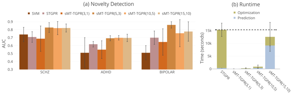
Figure 1: Comparison between ST-GPR and sMT-GPTR in terms of: a) AUC in the abnormal sample detection using normative modeling, and b) optimization and prediction runtime. The numbers in the parentheses show the number of components used in tensor factorization of $\hat{\mathcal{Z}}$ and $\hat{\mathcal{E}}$.

3.2 sMT-GPTR: Faster, More Accurate, and Feasible in Whole-Brain Inference

Figure 1 compares the AUC and runtime of ST-GPR with those of sMT-GPTR for different numbers of components in tensor factorization. As illustrated in Figure 1(a), accounting for spatial structures of the signal and noise in the multi-task learning setting provides normative models with better detection accuracy relative to single-task learning. Using sufficient components in the tensor factorization, the sMT-GPTR approach provides substantially higher accuracy in detecting abnormal samples across all diagnosis labels. Considering the fact that ST-GPR and sMT-GPTR models showed similar regression performance (see supplement), the AUC boost in sMT-GPTR models probably reflect better estimations of epistemic and aleatoric uncertainties. Our results show that using sMT-GPTR with 5 and 3 components to respectively explain the variances of the random-effect and noise is enough to reach the highest detection accuracy.

The gain in the detection accuracy is even more pronounced in comparison with the supervised SVM classifier. SVM achieves inferior AUC ($0.74\pm 0.09$) compared to our unsupervised approach in classifying SCHZ patients and its performance remains at the chance-level in ADHD and BIPL cases. The fact that our approach outperforms a fully supervised approach despite never having seen a patient indicates that the target pattern is not consistent across individuals within the patient group (Wolfers et al.,, 2015). Instead, the normative model focuses only on estimating the healthy distribution and can detect differences from this distribution regardless of whether they are consistent with one another. Moreover, in the supervised scenario, even though the model has access to labels, it cannot benefit from the information in the covariates. While in the normative modeling framework both sources of information (in covariates and fMRI data) are exploited.

In addition to making multi-task learning possible in a very high-dimensional setting, for a reasonable number of components, sMT-GPTR is significantly faster than ST-GPR in terms of total runtime (Fig. 1(b)). For example, sMT-GPTR(10,5) is 17 times faster than ST-GPR reducing its runtime from $\sim 4$ hours to $\sim 15$ minutes. Even though the model selection process to decide the number of components is a time-consuming step in practice, due to the low running time of the proposed approach, it remains economical compared to other multi-task alternatives. It the end, it is worthwhile to emphasize that these improvements are achieved by reducing the degree-of-freedom of the normative model from 597800 for ST-GPR to $29+6=35$ for sMT-GPTR (see Table 1 for the number of parameters and hyperparameters of different models).

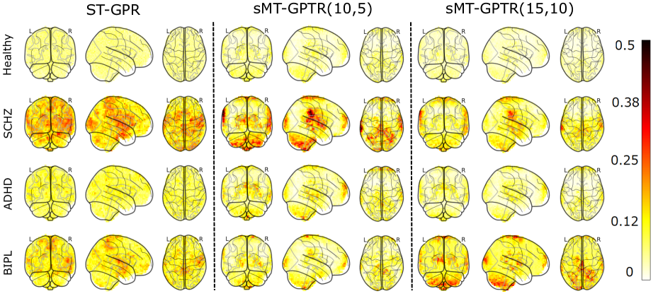
Figure 2: The probability of each voxel to deviate from the normative model in healthy and patient populations; derived by ST-GPR, sMT-GPTR(10,5), and sMT-GPTR(15,10).

3.3 Understanding the Underlying Neural Patterns of Abnormality

We have shown that accounting for spatial structure provides more accurate normative models than the baseline single-task model. However, it is also important to understand the neural basis of the underlying abnormalities. To achieve this for ST-GPR and sMT-GPTR, we use a spatial mixture model (Woolrich et al.,, 2005) to translate the corresponding NPM and S-NPM of each subject to a probability map, where the value of each voxel represents the probability that voxel deviates from the normative model (Wolfers et al.,, 2016). Figure 2 shows the resulting probability maps for ST-GPR, sMT-GPTR(10,5), and sMT-GPTR(15,10) averaged across runs and the healthy/patients population in the test set. These maps illustrate that: i) in general the probability of deviating from the normative model is higher in patients than healthy subjects. These deviations are more salient in SCHZ and BIPL patients compared to ADHD patients. This obseravation is compatible with higher novelty detection performance in SCHZ and BIPL patients (see Figure 1(a)); ii) the areas with high deviation probability are more spatially focal in sMT-GPTR models than the ST-GPR model. This suggests that the sMT-GPTR approach is better able to focus on the core abnormalities underlying the disorder and that accounting for spatial structure in both random-effect and noise provides a better estimation of the structured epistemic and aleatoric uncertainties in sMT-GPTR compared to ST-GPR models.

4 Related Work

Hyun et al., (2014, 2016) introduced spatial and spatio-temporal Gaussian predictive process to model neuroimaging data. They used functional principal component analysis to approximate the spatial/temporal covariance matrix of the random-effect combined with a multivariate autoregressive model for the noise. Their approach focuses on point estimation of outputs and does not provide a practical solution to estimate predictive uncertainty, thus cannot be employed for normative modeling. Our TGPP framework resolves this issue, and further, due to its flexible and general tensor assumption on the data structure, can be extended to other possible dimensions of neuroimaging data in addition to space and time.

Shvartsman et al., (2018) reformulated common fMRI analysis methods, such as representational similarity analysis, using matrix-variate normal formalism resulting in a unified framework for fMRI data analysis. They theoretically and experimentally showed the potentials of matrix-normal assumption on fMRI data in simultaneously modeling spatial and temporal noise covariances. Although our aim is different, our tensor-variate normal assumption on the distribution of the random-effect and noise can be seen as an extension of their approach, extending theoretical concepts in the multi-way modeling of neuroimaging data from 2-dimensional matrix-structured to $D$-dimensional tensor-structured data.

Exploiting the properties of Kronecker algebra to scale up the computational complexities of GPR in analyzing multi-way data is well studied in machine learning literature (Saatçi,, 2012; Wilson et al.,, 2014; Wilson and Nickisch,, 2015; Gilboa et al.,, 2015; Izmailov et al.,, 2018). However, all studies in this direction are mainly focus on multi-way input space, (i.e., single-task GPR), whereas we extend this ideas to multi-way output space, (i.e., multi-task GPR). This extension is one of our core contributions that makes the multivariate normative modeling possible.

The idea of using a sum of Kronecker products as the covariance term in order to concurrently learn structured signal and noise covariance functions in a multi-task Gaussian process setting is introduced first time in Rakitsch et al., (2013), known as GP-Kronsum. We have extended their method from two important perspectives: i) MT-GPTR generalizes the core idea of learning structured signal and noise covariance matrices to D-dimensional multi-way tensor structured data. This generalization not only provides the possibility of learning more complex multi-way structures but also reduces the computational complexities of GP-Kronsum by utilizing a more fine-grained Kronecker structure across different tensor dimensions; ii) we analytically show how using tensor factorization technique for low-rank approximation of covariance matrices can respectively decrease the time and space complexity of GP-Kronsum from $\mathcal{O}(T^{3})$ and $\mathcal{O}(T^{2})$ to $\mathcal{O}(T^{2})$ and $\mathcal{O}(T)$, i.e., one order of magnitude improvement. These massive improvements are crucial especially for applications on high-dimensional neuroimaging data.

5 Summary, Limitation, and Future Work

In this study, assuming a tensor-variate normal distribution on multi-way neuroimaging data and in a novel tensor Gaussian predictive process framework, we introduced a scalable multi-task Gaussian process tensor regression approach to model multi-way structured random-effect and noise on very high-dimensional neuroimaging data. The proposed approach provides a breakthrough toward practical modeling different sources of variations across different dimensions of large neuroimaging cohorts. On a clinical fMRI dataset, we exemplified one possible application of the proposed method for multivariate normative modeling of spatially distributed effects at the whole-brain level. We demonstrated that our framework provides more accurate results with reasonable computational costs, and it focuses better on the core underlying brain abnormalities relative to its mass-univariate alternative.

Due to its tensor-based design, the presented TGPP framework needs full-grid data across space, and/or other possible dimensions of neuroimaging data. This can be considered as a possible limitation when dealing with data with missing values across some data dimensions. One possible future direction is to solve this problem by imputing the grid using imaginary observations (Wilson et al.,, 2014; Wilson and Nickisch,, 2015). For future work, we aim to better understand the neuroscientific basis for the performance improvements we report (e.g., across multiple model orders and using different representations of the normative probability maps) and will apply the proposed method to very large cohorts in order to provide a more comprehensive model of biological variation in human brain.

Supplementary Materials

Throughout the supplementary materials we use the same notation introduced in the main text.

Useful Equations

For $\mathbf{A}\in\mathbb{R}^{M\times N}$, $\mathbf{B}\in\mathbb{R}^{P\times Q}$, and $\mathbf{C}$, $\mathbf{D}$ (with appropriate size) we have:

1. $\mathbf{A=U_{A}S_{A}U_{A}^{\top}}$ is the eigenvalue decomposition of $\mathbf{A}$,

2. $\mathbf{(ACB)^{-1}=B^{-1}C^{-1}A^{-1}}$,

3. $\mathbf{(A\otimes B)(C\otimes D)=AC\otimes BD}$,

4. $\mathbf{(A\otimes B)^{-1}=A^{-1}\otimes B^{-1}}$,

5. the eigenvalue decomposition of $\mathbf{A\otimes B+I}$ is: $\mathbf{(U_{A}\otimes U_{B})(S_{A}\otimes S_{B}+I)(U_{A}^{\top}\otimes U_{B}^{\top})}$,

6. $(\mathbf{A\otimes B})vec(\mathbf{C})=vec(\mathbf{BCA}^{\top})$,

7. $\ln\left|\mathbf{AC}\right|=\ln(\left|\mathbf{A}\right|\left|\mathbf{C}\right|)=\ln\left|\mathbf{A}\right|+\ln\left|\mathbf{C}\right|$,

8. for $\mathbf{C}\in\mathbb{R}^{N\times N}$, $\frac{\mathrm{d}}{\mathrm{d}x}\ln\left|\mathbf{C}\right|=Tr[\mathbf{C}^{-1}\frac{\mathrm{d}\mathbf{C}}{\mathrm{d}x}]$,

9. $Tr[\mathbf{ACBD}]=Tr[\mathbf{CBDA}]=Tr[\mathbf{BDAC}]=Tr[\mathbf{DACB}]$,

10. $Tr[\mathbf{A^{\top}C}]=vec(C)^{\top}vec(A)$,

11. $\ln\left|\mathbf{C}\otimes\mathbf{D}\right|=M\ln\left|\mathbf{C}\right|+N\ln\left|\mathbf{D}\right|,\quad for\quad\mathbf{C}\in\mathbb{R}^{N\times N},\mathbf{D}\in\mathbb{R}^{M\times M}$,

12. $\ln\left|diag(\mathbf{C})\right|=\prod_{i=1}^{N}\mathbf{C}[i,i],\quad for\quad\mathbf{C}\in\mathbb{R}^{N\times N}$.

Tensor Normal Distribution for $\mathcal{Z}^{\prime}$

Eq. 4 is derived as follows:

$$\begin{split}&p(\mathcal{Z^{\prime}}\mid\mathbf{C}_{i}\mid_{i=1}^{D},\mathbf{R})=\mathcal{TN}(\mathbf{0},\bigotimes_{i=1}^{D}\mathbf{C}_{i}\otimes\mathbf{R})=\frac{\exp(-\frac{1}{2}vec(\mathcal{Z^{\prime}})^{\top}[\bigotimes_{i=1}^{D}\mathbf{C}_{i}\otimes\mathbf{R}]^{-1}vec(\mathcal{Z^{\prime}}))}{\sqrt{(2\pi)^{N\prod_{i=1}^{D}P_{i}}\left|\bigotimes_{i=1}^{D}\mathbf{C}_{i}\right|^{N}\left|\mathbf{R}\right|^{\prod_{i=1}^{D}P_{i}}}}=\\ &\frac{\exp(-\frac{1}{2}vec(\mathcal{Z^{\prime}})^{\top}vec(\mathbf{R}^{-1}\mathbf{Z^{\prime}_{(1)}}\bigotimes_{i=1}^{D}\mathbf{C}_{i}^{-1}))}{\sqrt{(2\pi)^{N\prod_{i=1}^{D}P_{i}}\left|\bigotimes_{i=1}^{D}\mathbf{C}_{i}\right|^{N}\left|\mathbf{R}\right|^{\prod_{i=1}^{D}P_{i}}}}=\frac{\exp(-\frac{1}{2}Tr[\bigotimes_{i=1}^{D}\mathbf{C}_{i}^{-1}\mathbf{Z^{\prime\top}_{(1)}\mathbf{R}^{-1}\mathbf{Z^{\prime}}_{(1)}}])}{\sqrt{(2\pi)^{N\prod_{i=1}^{D}P_{i}}\left|\bigotimes_{i=1}^{D}\mathbf{C}_{i}\right|^{N}\left|\mathbf{R}\right|^{\prod_{i=1}^{D}P_{i}}}}\\ &\xrightarrow[]{\mathbf{Z^{\prime}_{(1)}}=\mathbf{\hat{Z}_{(1)}}(\bigotimes_{i=1}^{D}\mathbf{B}_{i}^{\top})^{-1}}\frac{\exp(-\frac{1}{2}Tr[\bigotimes_{i=1}^{D}\mathbf{C}_{i}^{-1}\bigotimes_{i=1}^{D}\mathbf{B}_{i}^{\dagger}\mathbf{\hat{Z}_{(1)}}^{\top}\mathbf{R}^{-1}\mathbf{\hat{Z}_{(1)}}(\bigotimes_{i=1}^{D}\mathbf{B}_{i}^{\top})^{-1}])}{\sqrt{(2\pi)^{N\prod_{i=1}^{D}P_{i}}\left|\bigotimes_{i=1}^{D}\mathbf{C}_{i}\right|^{N}\left|\mathbf{R}\right|^{\prod_{i=1}^{D}P_{i}}}}=\\ &\frac{\exp(-\frac{1}{2}Tr[\bigotimes_{i=1}^{D}\mathbf{B}_{i}\mathbf{C}_{i}^{-1}\mathbf{B}_{i}^{\top}\mathbf{\hat{Z}_{(1)}}^{\top}\mathbf{R}^{-1}\mathbf{\hat{Z}_{(1)}}])}{\sqrt{(2\pi)^{N\prod_{i=1}^{D}P_{i}}\left|\bigotimes_{i=1}^{D}\mathbf{C}_{i}\right|^{N}\left|\mathbf{R}\right|^{\prod_{i=1}^{D}P_{i}}}}\quad.\end{split}$$

Efficient Mean Prediction

Eq. 9(a) is derived from Eq. 8(a) as follows:

$$\begin{split}vec(\mathcal{M}^{*})=&(\bigotimes_{i=1}^{D}\mathbf{B}_{i}\mathbf{C}_{i}\mathbf{B}_{i}^{\top}\otimes\mathbf{R}^{*})(\bigotimes_{i=1}^{D}\mathbf{B}_{i}\mathbf{C}_{i}\mathbf{B}_{i}^{\top}\otimes\mathbf{R}+\bigotimes_{i=1}^{D}\mathbf{\Lambda}_{i}\mathbf{\Sigma}_{i}\mathbf{\Lambda}_{i}^{\top}\otimes\mathbf{\Omega})^{-1}vec(\mathcal{Y})\\ =&(\bigotimes_{i=1}^{D}\mathbf{B}_{i}\mathbf{C}_{i}\mathbf{B}_{i}^{\top}\otimes\mathbf{R}^{*})(\bigotimes_{i=1}^{D}\mathbf{B}_{i}\mathbf{C}_{i}\mathbf{B}_{i}^{\top}\otimes\mathbf{R}+\bigotimes_{i=1}^{D}\mathbf{\Lambda}_{i}\mathbf{U_{\Sigma_{i}}S_{\Sigma_{i}}U_{\Sigma_{i}}^{\top}}\mathbf{\Lambda}_{i}^{\top}\otimes\mathbf{U_{\Omega}S_{\Omega}U_{\Omega}^{\top}})^{-1}vec(\mathcal{Y})\\ =&(\bigotimes_{i=1}^{D}\mathbf{B}_{i}\mathbf{C}_{i}\mathbf{B}_{i}^{\top}\otimes\mathbf{R}^{*})(\bigotimes_{i=1}^{D}\mathbf{\Lambda}_{i}\mathbf{U_{\Sigma_{i}}S_{\Sigma_{i}}^{-0.5}}\otimes\mathbf{U_{\Omega}S_{\Omega}^{-0.5}})(\bigotimes_{i=1}^{D}\mathbf{\tilde{C}_{i}}\otimes\mathbf{\tilde{R}}+\mathbf{I})^{-1}\\ &(\bigotimes_{i=1}^{D}\mathbf{S_{\Sigma_{i}}^{-0.5}U_{\Sigma_{i}}^{\top}\Lambda_{i}^{\top}}\otimes\mathbf{S_{\Omega}^{-0.5}U_{\Omega}^{\top}})vec(\mathcal{Y})\\ =&(\bigotimes_{i=1}^{D}\mathbf{B}_{i}\mathbf{C}_{i}\mathbf{B}_{i}^{\top}\mathbf{\Lambda}_{i}\mathbf{U_{\Sigma_{i}}S_{\Sigma_{i}}^{-0.5}}\otimes\mathbf{R}^{*}\mathbf{U_{\Omega}S_{\Omega}^{-0.5}})(\bigotimes_{i=1}^{D}\mathbf{U_{\tilde{C}_{i}}}\otimes\mathbf{U_{\tilde{R}}})(\bigotimes_{i=1}^{D}\mathbf{S_{\tilde{C}_{i}}}\otimes\mathbf{S_{\tilde{R}}}+\mathbf{I})^{-1}\\ &(\bigotimes_{i=1}^{D}\mathbf{U_{\tilde{C}_{i}}^{\top}}\otimes\mathbf{U_{\tilde{R}}^{\top}})vec(\mathbf{S_{\Omega}^{-0.5}U_{\Omega}^{\top}Y_{(1)}}\bigotimes_{i=1}^{D}\mathbf{\Lambda}_{i}\mathbf{U_{\Sigma_{i}}S_{\Sigma_{i}}^{-0.5}})\\ =&(\bigotimes_{i=1}^{D}\mathbf{B}_{i}\mathbf{C}_{i}\mathbf{B}_{i}^{\top}\mathbf{\Lambda}_{i}\mathbf{U_{\Sigma_{i}}S_{\Sigma_{i}}^{-0.5}}\otimes\mathbf{R}^{*}\mathbf{U_{\Omega}S_{\Omega}^{-0.5}})(\bigotimes_{i=1}^{D}\mathbf{U_{\tilde{C}_{i}}}\otimes\mathbf{U_{\tilde{R}}})vec(\mathbf{\tilde{Y}})\\ =&(\bigotimes_{i=1}^{D}\mathbf{B}_{i}\mathbf{C}_{i}\mathbf{B}_{i}^{\top}\mathbf{\Lambda}_{i}\mathbf{U_{\Sigma_{i}}S_{\Sigma_{i}}^{-0.5}}\otimes\mathbf{R}^{*}\mathbf{U_{\Omega}S_{\Omega}^{-0.5}})vec(\mathbf{U_{\tilde{R}}}\mathbf{\tilde{Y}}\bigotimes_{i=1}^{D}\mathbf{U_{\tilde{C}_{i}}^{\top}})\\ =&\mathbf{R^{*}U_{\Omega}S_{\Omega}^{-0.5}U_{\tilde{R}}\tilde{Y}\bigotimes_{i=1}^{D}U^{\top}_{\tilde{C}_{i}}S^{-0.5}_{\Sigma_{i}}U^{\top}_{\Sigma_{i}}\Lambda^{\top}_{i}B_{i}C_{i}B_{i}^{\top}}\quad.\end{split}$$

Efficient Variance Prediction

Eq. 9(b) is derived from Eq. 8(b) as follows:

$$\begin{split}\mathbf{V}^{*}=&(\bigotimes_{i=1}^{D}\mathbf{B}_{i}\mathbf{C}_{i}\mathbf{B}_{i}^{\top}\otimes\mathbf{R}^{**})-(\bigotimes_{i=1}^{D}\mathbf{B}_{i}\mathbf{C}_{i}\mathbf{B}_{i}^{\top}\otimes\mathbf{R}^{*})(\bigotimes_{i=1}^{D}\mathbf{B}_{i}\mathbf{C}_{i}\mathbf{B}_{i}^{\top}\otimes\mathbf{R}+\bigotimes_{i=1}^{D}\mathbf{\Lambda}_{i}\mathbf{\Sigma}_{i}\mathbf{\Lambda}_{i}^{\top}\otimes\mathbf{\Omega})^{-1}\\ &(\bigotimes_{i=1}^{D}\mathbf{B}_{i}\mathbf{C}_{i}\mathbf{B}_{i}^{\top}\otimes\mathbf{R}^{*\top})\\ =&(\bigotimes_{i=1}^{D}\mathbf{B}_{i}\mathbf{C}_{i}\mathbf{B}_{i}^{\top}\otimes\mathbf{R}^{**})-(\bigotimes_{i=1}^{D}\mathbf{B}_{i}\mathbf{C}_{i}\mathbf{B}_{i}^{\top}\otimes\mathbf{R}^{*})(\bigotimes_{i=1}^{D}\mathbf{\Lambda}_{i}\mathbf{U_{\Sigma_{i}}S_{\Sigma_{i}}^{-0.5}}\otimes\mathbf{U_{\Omega}S_{\Omega}^{-0.5}})\\ &(\bigotimes_{i=1}^{D}\mathbf{\tilde{C}_{i}}\otimes\mathbf{\tilde{R}}+\mathbf{I})^{-1}(\bigotimes_{i=1}^{D}\mathbf{S_{\Sigma_{i}}^{-0.5}U_{\Sigma_{i}}^{\top}\Lambda_{i}^{\top}}\otimes\mathbf{S_{\Omega}^{-0.5}U_{\Omega}^{\top}})(\bigotimes_{i=1}^{D}\mathbf{B}_{i}\mathbf{C}_{i}\mathbf{B}_{i}^{\top}\otimes\mathbf{R}^{*\top})\\ =&(\bigotimes_{i=1}^{D}\mathbf{B}_{i}\mathbf{C}_{i}\mathbf{B}_{i}^{\top}\otimes\mathbf{R}^{**})-(\bigotimes_{i=1}^{D}\mathbf{B}_{i}\mathbf{C}_{i}\mathbf{B}_{i}^{\top}\mathbf{\Lambda}_{i}\mathbf{U_{\Sigma_{i}}S_{\Sigma_{i}}^{-0.5}}\otimes\mathbf{R}^{*}\mathbf{U_{\Omega}S_{\Omega}^{-0.5}})\\ &(\bigotimes_{i=1}^{D}\mathbf{U_{\tilde{C}_{i}}}\otimes\mathbf{U_{\tilde{R}}})(\bigotimes_{i=1}^{D}\mathbf{S_{\tilde{C}_{i}}}\otimes\mathbf{S_{\tilde{R}}}+\mathbf{I})^{-1}(\bigotimes_{i=1}^{D}\mathbf{U_{\tilde{C}_{i}}^{\top}}\otimes\mathbf{U_{\tilde{R}}^{\top}})(\bigotimes_{i=1}^{D}\mathbf{S_{\Sigma_{i}}^{-0.5}U_{\Sigma_{i}}^{\top}\Lambda_{i}^{\top}}\mathbf{B}_{i}\mathbf{C}_{i}\mathbf{B}_{i}^{\top}\otimes\mathbf{S_{\Omega}^{-0.5}U_{\Omega}^{\top}}\mathbf{R}^{*\top})\\ =&\mathbf{(\bigotimes_{i=1}^{D}B_{i}C_{i}B_{i}^{\top}\otimes R^{**})-(\bigotimes_{i=1}^{D}B_{i}C_{i}B_{i}^{\top}\Lambda_{i}U_{\Sigma_{i}}S_{\Sigma_{i}}^{-0.5}U_{\tilde{C}_{i}}\otimes R^{*}U_{\Omega}S_{\Omega}^{-0.5}U_{\tilde{R}})}\\ &\mathbf{(\bigotimes_{i=1}^{D}S_{\tilde{C}_{i}}\otimes S_{\tilde{R}}+I)^{-1}(\bigotimes_{i=1}^{D}U^{\top}_{\tilde{C}_{i}}S^{-0.5}_{\Sigma_{i}}U^{\top}_{\Sigma_{i}}\Lambda^{\top}_{i}B_{i}C_{i}B_{i}^{\top}\otimes U_{\tilde{R}}^{\top}S_{\Omega}^{-0.5}U_{\Omega}^{\top}R^{*\top})}\quad.\end{split}$$

Efficient Log Marginal Likelihood Evaluation

Eq. 10 is derived as follows:

$$\begin{split}&L=-\frac{NT}{2}\ln(2\pi)-\frac{1}{2}\ln\left|\mathbf{K}\right|-\frac{1}{2}vec(\mathbf{Y})^{\top}\mathbf{K}^{-1}vec(\mathbf{Y})\\ &=-\frac{NT}{2}\ln(2\pi)-\frac{1}{2}\ln\left|\bigotimes_{i=1}^{D}\mathbf{B}_{i}\mathbf{C}_{i}\mathbf{B}_{i}^{\top}\otimes\mathbf{R}+\bigotimes_{i=1}^{D}\mathbf{\Lambda}_{i}\mathbf{\Sigma}_{i}\mathbf{\Lambda}_{i}^{\top}\otimes\mathbf{\Omega}\right|-\\ &\frac{1}{2}vec(\mathbf{Y})^{\top}(\bigotimes_{i=1}^{D}\mathbf{B}_{i}\mathbf{C}_{i}\mathbf{B}_{i}^{\top}\otimes\mathbf{R}+\bigotimes_{i=1}^{D}\mathbf{\Lambda}_{i}\mathbf{\Sigma}_{i}\mathbf{\Lambda}_{i}^{\top}\otimes\mathbf{\Omega})^{-1}vec(\mathbf{Y})\\ &=-\frac{NT}{2}\ln(2\pi)-\frac{1}{2}\ln\left|(\bigotimes_{i=1}^{D}\mathbf{\Lambda}_{i}\mathbf{U_{\Sigma_{i}}S_{\Sigma_{i}}^{-0.5}}\otimes\mathbf{U_{\Omega}S_{\Omega}^{-0.5}})(\bigotimes_{i=1}^{D}\mathbf{\tilde{C}_{i}}\otimes\mathbf{\tilde{R}}+\mathbf{I})^{-1}(\bigotimes_{i=1}^{D}\mathbf{S_{\Sigma_{i}}^{-0.5}U_{\Sigma_{i}}^{\top}\Lambda_{i}^{\top}}\otimes\mathbf{S_{\Omega}^{-0.5}U_{\Omega}^{\top}})\right|-\\ &\frac{1}{2}vec(\mathbf{Y})^{\top}[(\bigotimes_{i=1}^{D}\mathbf{\Lambda}_{i}\mathbf{U_{\Sigma_{i}}S_{\Sigma_{i}}^{-0.5}}\otimes\mathbf{U_{\Omega}S_{\Omega}^{-0.5}})(\bigotimes_{i=1}^{D}\mathbf{\tilde{C}_{i}}\otimes\mathbf{\tilde{R}}+\mathbf{I})^{-1}(\bigotimes_{i=1}^{D}\mathbf{S_{\Sigma_{i}}^{-0.5}U_{\Sigma_{i}}^{\top}\Lambda_{i}^{\top}}\otimes\mathbf{S_{\Omega}^{-0.5}U_{\Omega}^{\top}})]vec(\mathbf{Y})\\ &=-\frac{NT}{2}\ln(2\pi)-\frac{1}{2}\ln\left|\bigotimes_{i=1}^{D}\mathbf{\Lambda}_{i}\mathbf{U_{\Sigma_{i}}S_{\Sigma_{i}}U_{\Sigma_{i}}^{\top}}\mathbf{\Lambda}_{i}^{\top}\otimes\mathbf{U_{\Omega}S_{\Omega}U_{\Omega}^{\top}}\right|-\frac{1}{2}\ln\left|\bigotimes_{i=1}^{D}\mathbf{S_{\tilde{C}_{i}}}\otimes\mathbf{S_{\tilde{R}}}+\mathbf{I}\right|\\ &-\frac{1}{2}vec(\mathbf{S_{\Omega}^{-0.5}U_{\Omega}^{\top}Y_{(1)}}\bigotimes_{i=1}^{D}\mathbf{\Lambda}_{i}\mathbf{U_{\Sigma_{i}}S_{\Sigma_{i}}^{-0.5}})^{\top}(\bigotimes_{i=1}^{D}\mathbf{U_{\tilde{C}_{i}}}\otimes\mathbf{U_{\tilde{R}}})(\bigotimes_{i=1}^{D}\mathbf{S_{\tilde{C}_{i}}}\otimes\mathbf{S_{\tilde{R}}}+\mathbf{I})^{-1}\\ &(\bigotimes_{i=1}^{D}\mathbf{U_{\tilde{C}_{i}}^{\top}}\otimes\mathbf{U_{\tilde{R}}^{\top}})vec(\mathbf{S_{\Omega}^{-0.5}U_{\Omega}^{\top}Y_{(1)}}\bigotimes_{i=1}^{D}\mathbf{\Lambda}_{i}\mathbf{U_{\Sigma_{i}}S_{\Sigma_{i}}^{-0.5}})\\ &=-\frac{NT}{2}\ln(2\pi)-\frac{1}{2}\ln\left|\bigotimes_{i=1}^{D}\mathbf{S_{\Sigma_{i}}}\otimes\mathbf{S_{\Omega}}\right|-\frac{1}{2}\ln\left|\bigotimes_{i=1}^{D}\mathbf{S_{\tilde{C}_{i}}}\otimes\mathbf{S_{\tilde{R}}}+\mathbf{I}\right|-\frac{1}{2}vec(\mathbf{Y^{\prime}})^{\top}(\bigotimes_{i=1}^{D}\mathbf{S_{\tilde{C}_{i}}}\otimes\mathbf{S_{\tilde{R}}}+\mathbf{I})^{-1}vec(\mathbf{Y^{\prime}})\\ &=-\frac{NT}{2}\ln(2\pi)-\frac{N}{2}\sum_{j=1}^{T}(\ln\bigotimes_{i=1}^{D}\mathbf{S_{\Sigma_{i}}})[j,j]-\frac{T}{2}\sum_{j=1}^{N}(\ln\mathbf{S_{\Omega}}[j,j])-\frac{1}{2}\\ &\sum_{k=1}^{T}\sum_{j=1}^{N}\ln(\bigotimes_{i=1}^{D}\mathbf{S_{\tilde{C}_{i}}}[k,k]\mathbf{S_{\tilde{R}}}[j,j]+1)-\frac{1}{2}vec(\mathbf{Y^{\prime}})^{\top}(\bigotimes_{i=1}^{D}\mathbf{S_{\tilde{C}_{i}}\otimes S_{\tilde{R}}+I})^{-1}vec(\mathbf{Y^{\prime}})\quad.\end{split}$$

Derivatives of $L$ with Respect to Parameters

In the optimization process, the derivatives of $L$ with respect to $\theta_{\mathbf{C}_{i}}\in\Theta_{\mathbf{C}_{i}}$, $\theta_{\mathbf{\Sigma}_{i}}\in\Theta_{\mathbf{\Sigma}_{i}}$, $\theta_{\mathbf{R}}\in\Theta_{\mathbf{R}}$, and $\theta_{\mathbf{\Omega}}\in\Theta_{\mathbf{\Omega}}$ can be efficiently computed as follows:

Gradients of $L$ with Respect to $\theta_{\mathbf{C}_{i}}$

$$\begin{split}\frac{\partial L}{\partial\theta_{\mathbf{C}_{i}}}&=-\frac{1}{2}diag((\bigotimes_{k=1}^{D}\mathbf{S_{\tilde{C}_{k}}\otimes S_{\tilde{R}}+I})^{-1})^{\top}\\ &diag(\mathbf{S_{\tilde{C}_{1}}\otimes S_{\tilde{C}_{2}}\otimes\dots\otimes U_{\tilde{C}_{i}}^{\top}S^{-0.5}_{\Sigma_{i}}U^{\top}_{\Sigma_{i}}\Lambda^{\top}_{i}B_{i}\frac{\partial C_{i}}{\partial\theta_{\tilde{C}_{i}}}B_{i}^{\top}\Lambda_{i}U_{\Sigma_{i}}S^{-0.5}_{\Sigma_{i}}U_{\tilde{C}_{i}}\otimes\dots\otimes S_{\tilde{C}_{D}}\otimes S_{\tilde{R}}})\\ &+\frac{1}{2}vec(\mathbf{\tilde{Y}})^{\top}vec(\mathbf{S_{\tilde{R}}\tilde{Y}\mathbf{(S_{\tilde{C}_{1}}\otimes S_{\tilde{C}_{2}}\otimes\dots\otimes U_{\tilde{C}_{i}}^{\top}S^{-0.5}_{\Sigma_{i}}U^{\top}_{\Sigma_{i}}\Lambda^{\top}_{i}B_{i}\frac{\partial C_{i}}{\partial\theta_{\tilde{C}_{i}}}B_{i}^{\top}\Lambda_{i}U_{\Sigma_{i}}S^{-0.5}_{\Sigma_{i}}U_{\tilde{C}_{i}}\otimes\dots\otimes S_{\tilde{C}_{D}}})}),\end{split}$$

where the determinant term of the above equation is derived by computing the derivative of $\ln\left|\mathbf{K}\right|$:

$$\begin{split}&\frac{\partial\ln\left|\mathbf{K}\right|}{\partial\theta_{\mathbf{C}_{i}}}=\frac{\partial}{\partial\theta_{\mathbf{C}_{i}}}\ln\left|\bigotimes_{k=1}^{D}\mathbf{B}_{k}\mathbf{C}_{i}\mathbf{B}_{k}^{\top}\otimes\mathbf{R}+\bigotimes_{k=1}^{D}\mathbf{\Lambda}_{k}\mathbf{\Sigma}_{k}\mathbf{\Lambda}_{k}^{\top}\otimes\mathbf{\Omega}\right|\\ &=Tr[(\bigotimes_{k=1}^{D}\mathbf{B}_{k}\mathbf{C}_{k}\mathbf{B}_{k}^{\top}\otimes\mathbf{R}+\bigotimes_{k=1}^{D}\mathbf{\Lambda}_{k}\mathbf{\Sigma}_{k}\mathbf{\Lambda}_{k}^{\top}\otimes\mathbf{\Omega})^{-1}\frac{\partial}{\partial\theta_{\mathbf{C}_{i}}}(\bigotimes_{k=1}^{D}\mathbf{B}_{k}\mathbf{C}_{k}\mathbf{B}_{k}^{\top}\otimes\mathbf{R}+\bigotimes_{k=1}^{D}\mathbf{\Lambda}_{k}\mathbf{\Sigma}_{k}\mathbf{\Lambda}_{k}^{\top}\otimes\mathbf{\Omega})]\\ &=Tr[(\bigotimes_{k=1}^{D}\mathbf{\Lambda}_{k}\mathbf{U_{\Sigma_{k}}S_{\Sigma_{k}}^{-0.5}}\otimes\mathbf{U_{\Omega}S_{\Omega}^{-0.5}})(\bigotimes_{k=1}^{D}\mathbf{\tilde{C}_{k}}\otimes\mathbf{\tilde{R}}+\mathbf{I})^{-1}(\bigotimes_{k=1}^{D}\mathbf{S_{\Sigma_{k}}^{-0.5}U_{\Sigma_{k}}^{\top}\Lambda_{k}^{\top}}\otimes\mathbf{S_{\Omega}^{-0.5}U_{\Omega}^{\top}})\\ &(\bigotimes_{k=1}^{D}\mathbf{B}_{k}\frac{\partial\mathbf{C}}{\partial\theta_{\mathbf{C}_{i}}}\mathbf{B}_{k}^{\top}\otimes\mathbf{R})]\\ &=Tr[(\bigotimes_{k=1}^{D}\mathbf{\Lambda}_{k}\mathbf{U_{\Sigma_{k}}S_{\Sigma_{k}}^{-0.5}}\otimes\mathbf{U_{\Omega}S_{\Omega}^{-0.5}})(\bigotimes_{k=1}^{D}\mathbf{U_{\tilde{C}_{k}}}\otimes\mathbf{U_{\tilde{R}}})(\bigotimes_{k=1}^{D}\mathbf{S_{\tilde{C}_{k}}}\otimes\mathbf{S_{\tilde{R}}}+\mathbf{I})^{-1}(\bigotimes_{i=k}^{D}\mathbf{U_{\tilde{C}_{k}}^{\top}}\otimes\mathbf{U_{\tilde{R}}^{\top}})\\ &(\bigotimes_{k=1}^{D}\mathbf{S_{\Sigma_{k}}^{-0.5}U_{\Sigma_{k}}^{\top}\Lambda_{k}^{\top}}\otimes\mathbf{S_{\Omega}^{-0.5}U_{\Omega}^{\top}})(\bigotimes_{k=1}^{D}\mathbf{B}_{k}\frac{\partial\mathbf{C}}{\partial\theta_{\mathbf{C}_{i}}}\mathbf{B}_{k}^{\top}\otimes\mathbf{R})]\\ &=Tr[(\bigotimes_{k=1}^{D}\mathbf{S_{\tilde{C}_{k}}}\otimes\mathbf{S_{\tilde{R}}}+\mathbf{I})^{-1}(\bigotimes_{k=1}^{D}\mathbf{U_{\tilde{C}_{k}}^{\top}}\otimes\mathbf{U_{\tilde{R}}^{\top}})(\bigotimes_{k=1}^{D}\mathbf{S_{\Sigma_{k}}^{-0.5}U_{\Sigma_{k}}^{\top}\Lambda_{k}^{\top}}\otimes\mathbf{S_{\Omega}^{-0.5}U_{\Omega}^{\top}})\\ &(\bigotimes_{k=1}^{D}\mathbf{B}_{k}\frac{\partial\mathbf{C}}{\partial\theta_{\mathbf{C}_{i}}}\mathbf{B}_{k}^{\top}\otimes\mathbf{R})(\bigotimes_{k=1}^{D}\mathbf{\Lambda}_{k}\mathbf{U_{\Sigma_{k}}S_{\Sigma_{k}}^{-0.5}}\otimes\mathbf{U_{\Omega}S_{\Omega}^{-0.5}})(\bigotimes_{k=1}^{D}\mathbf{U_{\tilde{C}_{k}}}\otimes\mathbf{U_{\tilde{R}}})]\\ &=Tr[(\bigotimes_{k=1}^{D}\mathbf{S_{\tilde{C}_{k}}}\otimes\mathbf{S_{\tilde{R}}}+\mathbf{I})^{-1}(\bigotimes_{k=1}^{D}\mathbf{U_{\tilde{C}_{k}}^{\top}S_{\Sigma_{k}}^{-0.5}U_{\Sigma_{k}}^{\top}A_{k}^{\top}B_{k}\frac{\partial C_{k}}{\partial\theta_{C_{i}}}B_{k}^{\top}A_{k}U_{\Sigma_{k}}S_{\Sigma_{k}}^{-0.5}U_{\tilde{C}_{k}}}\\ &\otimes\mathbf{U_{\tilde{R}}^{\top}S_{\Omega}^{-0.5}U_{\Omega}^{\top}RU_{\Omega}S_{\Omega}^{-0.5}U_{\tilde{R}}})]=diag((\bigotimes_{k=1}^{D}\mathbf{S_{\tilde{C}_{k}}\otimes S_{\tilde{R}}+I})^{-1})^{\top}\\ &diag(\mathbf{S_{\tilde{C}_{1}}\otimes S_{\tilde{C}_{2}}\otimes\dots\otimes U_{\tilde{C}_{i}}^{\top}S^{-0.5}_{\Sigma_{i}}U^{\top}_{\Sigma_{i}}\Lambda^{\top}_{i}B_{i}\frac{\partial C_{i}}{\partial\theta_{\tilde{C}_{i}}}B_{i}^{\top}\Lambda_{i}U_{\Sigma_{i}}S^{-0.5}_{\Sigma_{i}}U_{\tilde{C}_{i}}\otimes\dots\otimes S_{\tilde{C}_{D}}\otimes S_{\tilde{R}}}),\end{split}$$

and for the squared term we have:

$$\begin{split}&\frac{\partial}{\partial\theta_{\mathbf{C}_{i}}}[vec(\mathbf{Y})^{\top}\mathbf{K}^{-1}vec(\mathbf{Y})]=vec(\mathbf{Y})^{\top}\frac{\partial\mathbf{K}^{-1}}{\partial\theta_{\mathbf{C}_{i}}}vec(\mathbf{Y})=-vec(\mathbf{Y})^{\top}\mathbf{K}^{-1}\frac{\partial\mathbf{K}}{\partial\theta_{\mathbf{C}_{i}}}\mathbf{K}^{-1}vec(\mathbf{Y})\\ &=-vec(\mathbf{Y})^{\top}(\bigotimes_{k=1}^{D}\mathbf{\Lambda}_{k}\mathbf{U_{\Sigma_{k}}S_{\Sigma_{k}}^{-0.5}}\otimes\mathbf{U_{\Omega}S_{\Omega}^{-0.5}})(\bigotimes_{k=1}^{D}\mathbf{U_{\tilde{C}_{k}}}\otimes\mathbf{U_{\tilde{R}}})(\bigotimes_{k=1}^{D}\mathbf{S_{\tilde{C}_{k}}}\otimes\mathbf{S_{\tilde{R}}}+\mathbf{I})^{-1}(\bigotimes_{i=k}^{D}\mathbf{U_{\tilde{C}_{k}}^{\top}}\otimes\mathbf{U_{\tilde{R}}^{\top}})\\ &(\bigotimes_{k=1}^{D}\mathbf{S_{\Sigma_{k}}^{-0.5}U_{\Sigma_{k}}^{\top}\Lambda_{k}^{\top}}\otimes\mathbf{S_{\Omega}^{-0.5}U_{\Omega}^{\top}})(\bigotimes_{k=1}^{D}\mathbf{\Lambda}_{k}\mathbf{U_{\Sigma_{k}}S_{\Sigma_{k}}^{0.5}}\otimes\mathbf{U_{\Omega}S_{\Omega}^{0.5}})\\ &(\bigotimes_{k=1}^{D}\frac{\partial\mathbf{\tilde{C}_{k}}}{\partial\theta_{\mathbf{C}_{i}}}\otimes\mathbf{\tilde{R}})(\bigotimes_{k=1}^{D}\mathbf{S_{\Sigma_{k}}^{0.5}U_{\Sigma_{k}}^{\top}\Lambda_{k}^{\top}}\otimes\mathbf{S_{\Omega}^{0.5}U_{\Omega}^{\top}})(\bigotimes_{k=1}^{D}\mathbf{\Lambda}_{k}\mathbf{U_{\Sigma_{k}}S_{\Sigma_{k}}^{-0.5}}\otimes\mathbf{U_{\Omega}S_{\Omega}^{-0.5}})\\ &(\bigotimes_{k=1}^{D}\mathbf{U_{\tilde{C}_{k}}}\otimes\mathbf{U_{\tilde{R}}})(\bigotimes_{k=1}^{D}\mathbf{S_{\tilde{C}_{k}}}\otimes\mathbf{S_{\tilde{R}}}+\mathbf{I})^{-1}(\bigotimes_{i=k}^{D}\mathbf{U_{\tilde{C}_{k}}^{\top}}\otimes\mathbf{U_{\tilde{R}}^{\top}})(\bigotimes_{k=1}^{D}\mathbf{S_{\Sigma_{k}}^{-0.5}U_{\Sigma_{k}}^{\top}\Lambda_{k}^{\top}}\otimes\mathbf{S_{\Omega}^{-0.5}U_{\Omega}^{\top}})vec(\mathbf{Y})\\ &=-vec(\mathbf{\tilde{Y}})^{\top}(\bigotimes_{k=1}^{D}\mathbf{U_{\tilde{C}_{k}}^{\top}}\otimes\mathbf{U_{\tilde{R}}^{\top}})(\bigotimes_{k=1}^{D}\frac{\partial\mathbf{\tilde{C}_{k}}}{\partial\theta_{\mathbf{C}_{i}}}\otimes\mathbf{\tilde{R}})(\bigotimes_{k=1}^{D}\mathbf{U_{\tilde{C}_{k}}}\otimes\mathbf{U_{\tilde{R}}})vec(\mathbf{\tilde{Y}})\\ &=-vec(\mathbf{\tilde{Y}})^{\top}(\bigotimes_{k=1}^{D}\mathbf{U_{\tilde{C}_{k}}^{\top}S_{\Sigma_{k}}^{-0.5}U_{\Sigma_{k}}^{\top}A_{k}^{\top}B_{k}\frac{\partial C_{k}}{\partial\theta_{C_{i}}}B_{k}^{\top}A_{k}U_{\Sigma_{k}}S_{\Sigma_{k}}^{-0.5}U_{\tilde{C}_{k}}\otimes S_{\tilde{R}}})vec(\mathbf{\tilde{Y}})\\ &=-vec(\mathbf{\tilde{Y}})^{\top}(\mathbf{S_{\tilde{R}}\tilde{Y}\bigotimes_{k=1}^{D}U_{\tilde{C}_{k}}^{\top}S_{\Sigma_{k}}^{-0.5}U_{\Sigma_{k}}^{\top}A_{k}^{\top}B_{k}\frac{\partial C_{k}}{\partial\theta_{C_{i}}}B_{k}^{\top}A_{k}U_{\Sigma_{k}}S_{\Sigma_{k}}^{-0.5}U_{\tilde{C}_{k}}})\\ &-vec(\mathbf{\tilde{Y}})^{\top}vec(\mathbf{S_{\tilde{R}}\tilde{Y}\mathbf{(S_{\tilde{C}_{1}}\otimes S_{\tilde{C}_{2}}\otimes\dots\otimes U_{\tilde{C}_{i}}^{\top}S^{-0.5}_{\Sigma_{i}}U^{\top}_{\Sigma_{i}}\Lambda^{\top}_{i}B_{i}\frac{\partial C_{i}}{\partial\theta_{\tilde{C}_{i}}}B_{i}^{\top}\Lambda_{i}U_{\Sigma_{i}}S^{-0.5}_{\Sigma_{i}}U_{\tilde{C}_{i}}\otimes\dots\otimes S_{\tilde{C}_{D}}})}).\end{split}$$

Gradients of $L$ with Respect to $\theta_{\mathbf{\Sigma}_{i}}$

$$\begin{split}&\frac{\partial L}{\partial\theta_{\mathbf{\Sigma}_{i}}}=-\frac{1}{2}diag((\bigotimes_{k=1}^{D}\mathbf{S_{\tilde{\Sigma}_{k}}\otimes S_{\tilde{\Omega}}+I})^{-1})^{\top}\\ &diag(\mathbf{S_{\tilde{\Sigma}_{1}}\otimes S_{\tilde{\Sigma}_{2}}\otimes\dots\otimes U_{\tilde{\Sigma}_{i}}^{\top}S^{-0.5}_{C_{i}}U^{\top}_{C_{i}}B^{\top}_{i}\Lambda_{i}\frac{\partial\Sigma_{i}}{\partial\theta_{\tilde{\Sigma}_{i}}}\Lambda_{i}^{\top}B_{i}U_{C_{i}}S^{-0.5}_{C_{i}}U_{\tilde{\Sigma}_{i}}\otimes\dots\otimes S_{\tilde{\Sigma}_{D}}\otimes S_{\tilde{\Omega}}})\\ &+\frac{1}{2}vec(\mathbf{\tilde{Y}})^{\top}vec(\mathbf{S_{\tilde{\Omega}}\tilde{Y}\mathbf{(S_{\tilde{\Sigma}_{1}}\otimes S_{\tilde{\Sigma}_{2}}\otimes\dots\otimes U_{\tilde{\Sigma}_{i}}^{\top}S^{-0.5}_{C_{i}}U^{\top}_{C_{i}}B^{\top}_{i}\Lambda_{i}\frac{\partial\Sigma_{i}}{\partial\theta_{\tilde{\Sigma}_{i}}}\Lambda_{i}^{\top}B_{i}U_{C_{i}}S^{-0.5}_{C_{i}}U_{\tilde{\Sigma}_{i}}\otimes\dots\otimes S_{\tilde{\Sigma}_{D}}})}),\end{split}$$

The derivation of the determinant and squared terms of $\frac{\partial L}{\partial\theta_{\mathbf{\Sigma}_{i}}}$ are similar to those of $\frac{\partial L}{\partial\theta_{\mathbf{C}_{i}}}$.

Gradients of $L$ with Respect to $\theta_{\mathbf{R}}$:

$$\begin{split}\frac{\partial L}{\partial\theta_{\mathbf{R}}}=&-\frac{1}{2}diag((\bigotimes_{k=1}^{D}\mathbf{S_{\tilde{C}_{k}}\otimes S_{\tilde{R}}+I})^{-1})^{\top}diag(\bigotimes_{k=1}^{D}\mathbf{S_{\tilde{C}_{k}}}\otimes\mathbf{U_{\tilde{R}}^{\top}S_{\Omega}^{-0.5}U_{\Omega}^{\top}}\frac{\partial\mathbf{R}}{\partial\theta_{\mathbf{R}}}\mathbf{U_{\Omega}S_{\Omega}^{-0.5}U_{\tilde{R}}})\\ &+\frac{1}{2}vec(\mathbf{\tilde{Y}})^{\top}vec(\mathbf{U_{\tilde{R}}^{\top}S_{\Omega}^{-0.5}U_{\Omega}^{\top}}\frac{\partial\mathbf{R}}{\partial\theta_{\mathbf{R}}}\mathbf{U_{\Omega}S_{\Omega}^{-0.5}U_{\tilde{R}}\tilde{Y}}\bigotimes_{k=1}^{D}\mathbf{S_{\tilde{C}_{k}}}).\end{split}$$

The derivation of the determinant and squared terms of $\frac{\partial L}{\partial\theta_{\mathbf{R}}}$ are similar to those of $\frac{\partial L}{\partial\theta_{\mathbf{C}_{i}}}$.

Gradients of $L$ with Respect to $\theta_{\mathbf{\Omega}}$:

$$\begin{split}\frac{\partial L}{\partial\theta_{\mathbf{\Omega}}}=&-\frac{1}{2}diag((\bigotimes_{k=1}^{D}\mathbf{S_{\tilde{\Sigma}_{k}}\otimes S_{\tilde{\Omega}}+I})^{-1})^{\top}diag(\bigotimes_{k=1}^{D}\mathbf{S_{\tilde{\Sigma}_{k}}}\otimes\mathbf{U_{\tilde{\Omega}}^{\top}S_{R}^{-0.5}U_{R}^{\top}}\frac{\partial\mathbf{\Omega}}{\partial\theta_{\mathbf{\Omega}}}\mathbf{U_{R}S_{R}^{-0.5}U_{\tilde{\Omega}}})\\ &+\frac{1}{2}vec(\mathbf{\tilde{Y}})^{\top}vec(\mathbf{U_{\tilde{\Omega}}^{\top}S_{R}^{-0.5}U_{R}^{\top}}\frac{\partial\mathbf{\Omega}}{\partial\theta_{\mathbf{\Omega}}}\mathbf{U_{R}S_{R}^{-0.5}U_{\tilde{\Omega}}\tilde{Y}}\bigotimes_{k=1}^{D}\mathbf{S_{\tilde{\Sigma}_{k}}}).\end{split}$$

The procedure to derive the determinant and squared terms of $\frac{\partial L}{\partial\theta_{\mathbf{\Omega}}}$ is similar to $\frac{\partial L}{\partial\theta_{\mathbf{C}_{i}}}$.

Comparing the Regression Performance

This figure summarizes the average regression performance ($R^{2}$) across all voxels for benchmarked approaches. All methods show similar performance in terms of the quality of regression. Note that the low $R^{2}$ values are due to averaging over all voxels that many are irrelevant to regressors in $\mathbf{X}$.

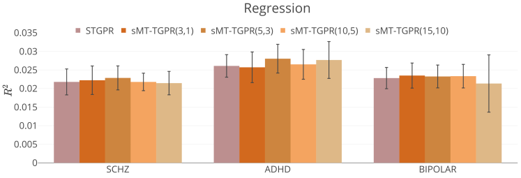
Figure 3: Comparison between ST-GPR and sMT-GPTR in terms of their regression performance.

Supplementary Deviation Maps

The following figure presents a complementary results for Sec. 3.3 of the main text.

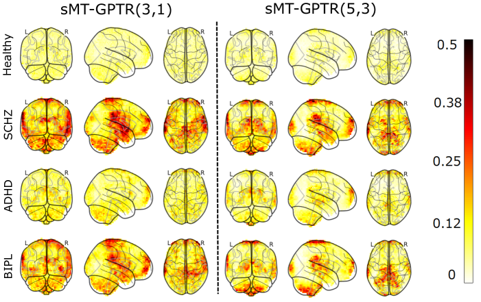
Figure 4: The probability of each voxel to deviate from the normative model in healthy and patient populations; derived by sMT-GPTR(3,1) and sMT-GPTR(5,3).

References

• Abraham et al., (2014) Abraham, A., Pedregosa, F., Eickenberg, M., Gervais, P., Mueller, A., Kossaifi, J., Gramfort, A., Thirion, B., and Varoquaux, G. (2014). Machine learning for neuroimaging with scikit-learn. Frontiers in Neuroinformatics, 8:14.
• Alvarez and Lawrence, (2009) Alvarez, M. and Lawrence, N. D. (2009). Sparse convolved Gaussian processes for multi-output regression. In Advances in neural information processing systems, pages 57–64.
• Álvarez and Lawrence, (2011) Álvarez, M. A. and Lawrence, N. D. (2011). Computationally efficient convolved multiple output Gaussian processes. Journal of Machine Learning Research, 12:1459–1500.
• Alvarez et al., (2010) Alvarez, M. A., Luengo, D., Titsias, M. K., and Lawrence, N. D. (2010). Efficient multioutput Gaussian processes through variational inducing kernels. In International Conference on Artificial Intelligence and Statistics, pages 25–32.
• Bonilla et al., (2008) Bonilla, E. V., Chai, K. M., and Williams, C. (2008). Multi-task Gaussian process prediction. In Advances in neural information processing systems, pages 153–160.
• Bowman et al., (2008) Bowman, F. D., Caffo, B., Bassett, S. S., and Kilts, C. (2008). A bayesian hierarchical framework for spatial modeling of fMRI data. NeuroImage, 39(1):146 – 156.
• Davison and Huser, (2015) Davison, A. C. and Huser, R. (2015). Statistics of extremes. Annual Review of Statistics and Its Application, 2(1):203–235.
• Foulkes and Blakemore, (2018) Foulkes, L. and Blakemore, S.-J. (2018). Studying individual differences in human adolescent brain development. Nature neuroscience, page 1.
• Friston et al., (1999) Friston, K. J., Holmes, A. P., Price, C., Büchel, C., and Worsley, K. (1999). Multisubject fMRI Studies and Conjunction Analyses. NeuroImage, 10(4):385 – 396.
• Gilboa et al., (2015) Gilboa, E., Saatçi, Y., and Cunningham, J. P. (2015). Scaling Multidimensional Inference for Structured Gaussian Processes. IEEE Transactions on Pattern Analysis and Machine Intelligence, 37(2):424–436.
• Gorgolewski et al., (2017) Gorgolewski, K. J., Durnez, J., and Poldrack, R. A. (2017). Preprocessed consortium for neuropsychiatric phenomics dataset [version 2; referees: 2 approved]. F1000Research, 6(1262).
• Gratton et al., (2018) Gratton, C., Laumann, T. O., Nielsen, A. N., Greene, D. J., Gordon, E. M., Gilmore, A. W., Nelson, S. M., Coalson, R. S., Snyder, A. Z., Schlaggar, B. L., et al. (2018). Functional brain networks are dominated by stable group and individual factors, not cognitive or daily variation. Neuron, 98(2):439–452.
• Hyun et al., (2014) Hyun, J. W., Li, Y., Gilmore, J. H., Lu, Z., Styner, M., and Zhu, H. (2014). Sgpp: spatial gaussian predictive process models for neuroimaging data. NeuroImage, 89:70 – 80.
• Hyun et al., (2016) Hyun, J. W., Li, Y., Huang, C., Styner, M., Lin, W., and Zhu, H. (2016). Stgp: Spatio-temporal gaussian process models for longitudinal neuroimaging data. NeuroImage, 134:550 – 562.
• Izmailov et al., (2018) Izmailov, P., Novikov, A., and Kropotov, D. (2018). Scalable gaussian processes with billions of inducing inputs via tensor train decomposition. In Storkey, A. and Perez-Cruz, F., editors, Proceedings of the Twenty-First International Conference on Artificial Intelligence and Statistics, volume 84 of Proceedings of Machine Learning Research, pages 726–735, Playa Blanca, Lanzarote, Canary Islands. PMLR.
• Kapur et al., (2012) Kapur, S., Phillips, A. G., and Insel, T. R. (2012). Why has it taken so long for biological psychiatry to develop clinical tests and what to do about it? Molecular psychiatry, 17(12):1174.
• Kendall and Gal, (2017) Kendall, A. and Gal, Y. (2017). What uncertainties do we need in bayesian deep learning for computer vision? In Advances in Neural Information Processing Systems, pages 5580–5590.
• Kolda and Bader, (2009) Kolda, T. G. and Bader, B. W. (2009). Tensor decompositions and applications. SIAM Review, 51(3):455–500.
• Kossaifi et al., (2016) Kossaifi, J., Panagakis, Y., and Pantic, M. (2016). Tensorly: Tensor learning in python. arXiv preprint arXiv:1610.09555.
• Loan, (2000) Loan, C. F. (2000). The ubiquitous kronecker product. Journal of Computational and Applied Mathematics, 123(1):85 – 100.
• Marquand et al., (2016) Marquand, A. F., Rezek, I., Buitelaar, J., and Beckmann, C. F. (2016). Understanding heterogeneity in clinical cohorts using normative models: beyond case-control studies. Biological psychiatry, 80(7):552–561.
• Mirnezami et al., (2012) Mirnezami, R., Nicholson, J., and Darzi, A. (2012). Preparing for Precision Medicine. New England Journal of Medicine, 366(6):489–491. PMID: 22256780.
• Mørup, (2011) Mørup, M. (2011). Applications of tensor (multiway array) factorizations and decompositions in data mining. Wiley Interdisciplinary Reviews: Data Mining and Knowledge Discovery, 1(1):24–40.
• Pedregosa et al., (2011) Pedregosa, F., Varoquaux, G., Gramfort, A., Michel, V., Thirion, B., Grisel, O., Blondel, M., Prettenhofer, P., Weiss, R., Dubourg, V., Vanderplas, J., Passos, A., Cournapeau, D., Brucher, M., Perrot, M., and Duchesnay, E. (2011). Scikit-learn: Machine learning in Python. Journal of Machine Learning Research, 12:2825–2830.
• Poldrack et al., (2016) Poldrack, R. A., Congdon, E., Triplett, W., Gorgolewski, K., Karlsgodt, K., Mumford, J., Sabb, F., Freimer, N., London, E., Cannon, T., et al. (2016). A phenome-wide examination of neural and cognitive function. Scientific data, 3:160110.
• Rakitsch et al., (2013) Rakitsch, B., Lippert, C., Borgwardt, K., and Stegle, O. (2013). It is all in the noise: Efficient multi-task Gaussian process inference with structured residuals. In Advances in neural information processing systems, pages 1466–1474.
• Roberts, (2000) Roberts, S. (2000). Extreme value statistics for novelty detection in biomedical data processing. IEE Proceedings - Science, Measurement and Technology, 147:363–367(4).
• Saatçi, (2012) Saatçi, Y. (2012). Scalable inference for structured Gaussian process models. PhD thesis, University of Cambridge.
• Shvartsman et al., (2018) Shvartsman, M., Sundaram, N., Aoi, M. C., Charles, A., Wilke, T. C., and Cohen, J. D. (2018). Matrix-normal models for fMRI analysis. In Proceedings of the 22th International Conference on Artificial Intelligence and Statistics. PMLR.
• Stegle et al., (2011) Stegle, O., Lippert, C., Mooij, J. M., Lawrence, N. D., and Borgwardt, K. M. (2011). Efficient inference in matrix-variate gaussian models with iid observation noise. In Advances in neural information processing systems, pages 630–638.
• Tucker, (1966) Tucker, L. R. (1966). Some mathematical notes on three-mode factor analysis. Psychometrika, 31(3):279–311.
• Williams and Rasmussen, (1996) Williams, C. K. and Rasmussen, C. E. (1996). Gaussian processes for regression. In Advances in neural information processing systems, pages 514–520.
• Wilson and Nickisch, (2015) Wilson, A. and Nickisch, H. (2015). Kernel Interpolation for Scalable Structured Gaussian Processes (KISS-GP). In Bach, F. and Blei, D., editors, Proceedings of the 32nd International Conference on Machine Learning, volume 37 of Proceedings of Machine Learning Research, pages 1775–1784, Lille, France. PMLR.
• Wilson et al., (2014) Wilson, A. G., Gilboa, E., Nehorai, A., and Cunningham, J. P. (2014). Fast kernel learning for multidimensional pattern extrapolation. In Advances in Neural Information Processing Systems, pages 3626–3634.
• Wolfers et al., (2015) Wolfers, T., Buitelaar, J. K., Beckmann, C. F., Franke, B., and Marquand, A. F. (2015). From estimating activation locality to predicting disorder: A review of pattern recognition for neuroimaging-based psychiatric diagnostics. Neuroscience and Biobehavioral Reviews, 57:328 – 349.
• Wolfers et al., (2016) Wolfers, T., van Rooij, D., Oosterlaan, J., Heslenfeld, D., Hartman, C. A., Hoekstra, P. J., Beckmann, C. F., Franke, B., Buitelaar, J. K., and Marquand, A. F. (2016). Quantifying patterns of brain activity: Distinguishing unaffected siblings from participants with adhd and healthy individuals. NeuroImage: Clinical, 12:227 – 233.
• Woolrich et al., (2005) Woolrich, M. W., Behrens, T. E. J., Beckmann, C. F., and Smith, S. M. (2005). Mixture models with adaptive spatial regularization for segmentation with an application to fMRI data. IEEE Transactions on Medical Imaging, 24(1):1–11.