The Measure and Mismeasure of Fairness
Abstract
The field of fair machine learning aims to ensure that decisions guided by algorithms are equitable. Over the last decade, several formal, mathematical definitions of fairness have gained prominence. Here we first assemble and categorize these definitions into two broad families: (1) those that constrain the effects of decisions on disparities; and (2) those that constrain the effects of legally protected characteristics, like race and gender, on decisions. We then show, analytically and empirically, that both families of definitions typically result in strongly Pareto dominated decision policies. For example, in the case of college admissions, adhering to popular formal conceptions of fairness would simultaneously result in lower student-body diversity and a less academically prepared class, relative to what one could achieve by explicitly tailoring admissions policies to achieve desired outcomes. In this sense, requiring that these fairness definitions hold can, perversely, harm the very groups they were designed to protect. In contrast to axiomatic notions of fairness, we argue that the equitable design of algorithms requires grappling with their context-specific consequences, akin to the equitable design of policy. We conclude by listing several open challenges in fair machine learning and offering strategies to ensure algorithms are better aligned with policy goals.
Keywords: Fair machine learning, consequentialism, discrimination
1 Introduction
In banking, criminal justice, medicine, and beyond, consequential decisions are often informed by machine learning algorithms (Chouldechova et al., 2018; Barocas and Selbst, 2016; Berk, 2012; Shroff, 2017). As the influence and scope of algorithms increase, academics, policymakers, and journalists have raised concerns that these tools might inadvertently encode and entrench human biases. Such concerns have sparked tremendous interest in developing fair machine-learning algorithms, and, accordingly, a plethora of formal fairness criteria have been proposed in the computer science community (Darlington, 1971; Cleary, 1968; Zafar et al., 2017b; Dwork et al., 2012; Chouldechova, 2017; Hardt et al., 2016; Kleinberg et al., 2017b; Woodworth et al., 2017; Zafar et al., 2017a; Corbett-Davies et al., 2017; Chouldechova and Roth, 2020; Berk et al., 2021; Coston et al., 2020; Imai and Jiang, 2020; Imai et al., 2020; Wang et al., 2019; Kusner et al., 2017; Nabi and Shpitser, 2018; Wu et al., 2019; Mhasawade and Chunara, 2021; Kilbertus et al., 2017; Zhang and Bareinboim, 2018; Zhang et al., 2017; Chiappa, 2019; Loftus et al., 2018; Galhotra et al., 2022; Carey and Wu, 2022). Here we synthesize and critically examine the statistical properties of popular formal fairness approaches as well as the consequences of enforcing them. Using both theory and empirical evidence, we argue that these approaches, when used as algorithmic design principles, can often cause more harm than good. In contrast to popular axiomatic approaches to algorithmic fairness, we advocate for a consequentialist perspective that directly grapples with the difficult policy trade-offs inherent to many algorithmically guided decisions.
We begin, in Section 2, by proposing a two-part taxonomy of formal fairness definitions. Our first category of definitions encompasses those that consider the effects of decisions on disparities. Imagine, for example, designing an algorithm to guide decisions for college admissions. Under the principle that fair algorithms should have comparable performance across demographic groups (Hardt et al., 2016), one might check that among applicants who were ultimately academically “successful” (e.g., who eventually earned a college degree, either at the institution in question or elsewhere), the algorithm would recommend admission for an equal proportion of candidates across race groups. Our second category of definitions encompasses those that seek to limit both the direct and indirect effects of one’s group membership on decisions. Following the principle that decisions should be agnostic to legally protected attributes like race and gender (cf. Dwork et al., 2012), one might mandate that these features not be provided to the algorithm. Further, because one’s race might impact earlier educational opportunities, and hence test scores, one might require that admissions decisions are robust to the effect of race along such causal paths.
These formalizations of fairness have considerable intuitive appeal. It can feel natural to exclude protected characteristics in a drive for equity; and one might understandably interpret disparities in error rates as indicating problems with an algorithm’s design or with the data on which it was trained. However, in Sections 3 and 4, we show that both classes of algorithmic fairness definitions suffer from deep statistical limitations. For example, for natural families of utility functions—like those that prefer both higher academic preparedness and more student-body diversity—we prove that common fairness criteria almost always, in a measure theoretic sense, lead to strongly Pareto dominated decision policies.111A policy is strongly Pareto dominated if there is an alternative feasible policy that is preferred under every utility function in the family (cf. Section 4.2). In particular, in our running college admissions example, adhering to several of the popular conceptions of fairness we consider would simultaneously result in lower student-body diversity and a less academically prepared class, relative to what one could attain by explicitly tailoring admissions policies to achieve desired outcomes. In fact, under one prominent definition of fairness, we prove that the induced policies require simply admitting all applicants with equal probability, irrespective of one’s academic qualifications or group membership. These formal fairness criteria are thus often at odds with policy goals, and, perversely, can harm the very same groups one ostensibly sought to protect by developing and adopting axiomatic notions of fairness.
How, then, can we ensure algorithms are fair? There are no easy solutions, but we conclude in Section 5 by offering several observations and suggestions for designing more equitable algorithms. Most importantly, we believe it is critical to acknowledge and tackle head-on the substantive trade-offs at the heart of many decision problems. For example, when creating a college admissions policy, one must necessarily make difficult choices that balance competing priorities. Formal fairness axioms are poor tools for engaging with these challenging issues. Our overarching exhortation is thus to recognize algorithms as encoding policy choices, and to accordingly tailor their design.
Contributions. To summarize, we offer three main contributions. First, we survey the fairness literature, describing existing fairness definitions and organizing them into a two-part taxonomy. Our categorization of formal fairness definitions proposed in the computer science literature highlights their connections to influential legal and economic notions of discrimination. Second, we lay out a consequentialist framework for designing equitable algorithms. Our framework is motivated by viewing algorithmic fairness as a policy objective rather than as a technical problem. This approach exposes the statistical and normative limitations of many popular formal fairness definitions. Finally, we apply our consequentialist framework to develop a positive vision for addressing problems of fairness and equity in algorithm design.
Much of the content we present synthesizes and builds on research that we and our collaborators have conducted over the last several years (Corbett-Davies et al., 2017; Cai et al., 2020; Chohlas-Wood et al., 2023a, b; Koenecke et al., 2023). In particular, we draw heavily on two papers by Corbett-Davies and Goel (2018) and Nilforoshan et al. (2022). In addition to synthesis, we broaden the formal theoretical results presented in this line of work and offer new, concrete illustrations of our theoretical arguments. Some of the results and arguments we present date back five years, and the field of algorithmic fairness has since moved forward in many ways. For example, in the intervening time, there has been increasing recognition of the shortcomings of popular formal fairness definitions (Barocas et al., 2019). Nevertheless, we believe our message is as relevant as ever. For instance, within the research community, new algorithmic fairness definitions are regularly introduced that, while different in some respects, frequently suffer from the same statistical and conceptual limitations as the notions we survey here. In the broader world, policymakers, algorithm designers, journalists, and advocates often still evaluate algorithms—and accordingly influence decisions—by turning to these formal fairness definitions without necessarily appreciating their shortcomings. For example, proposed legislation in Idaho sought to require that pretrial risk assessment algorithms have equal error rates across groups (Idaho H.B. 118, 2019). Although the proposed bill was never passed, it the illustrates the ways in which these formal measures have garnered significant attention beyond the academic community.
The call to build equitable algorithms will only grow over time as automated decisions become even more widespread. As such, it is imperative to address limitations in past formulations of fairness, to identify best practices moving forward, and to outline important open research questions. By synthesizing and critically examining recent developments in fair machine learning, we hope to help both researchers and practitioners advance this increasingly influential field.
2 Mathematical Definitions of Fairness
We start by assembling and categorizing definitions of algorithmic fairness into a two-part taxonomy: those that seek to limit the effect of decisions on disparities, and those that seek to limit the effect of protected attributes like race or gender on the decisions themselves. We first introduce formal notation and concrete examples of decision problems in which one might seek to apply these fairness definitions, before reviewing prominent examples of both approaches in turn.
2.1 Formal setting
Consider a population of individuals with observed covariates , drawn i.i.d. from a set with distribution . Further suppose that describes one or more discrete protected attributes, such as race or gender, which can be derived from (i.e., for some function ). Each individual is subject to a binary decision , determined by a (randomized) rule , where is the probability of receiving a positive decision, .222That is, , where is an independent uniform random variable on . ,333By “positive,” we simply mean the decision D is greater than zero, without ascribing any normative position to the decision. Individuals may or may not have a preferences for “positive” decisions in this sense. Given a budget with , we require the decision rule to satisfy . Finally, we suppose that each individual has some associated binary outcome . In some cases, we will be concerned with the causal effect of the decision on , in which case we imagine that there exist two potential outcomes, and , corresponding to what happens to the individual depending on whether they receive a negative or positive decision.444As is implicit in our notation, we assume that there are no spillover effects between units (Imbens and Rubin, 2015).
To make our discussion concrete, we imagine two running examples corresponding to this formal setting: diabetes screening and college admissions. As we discuss in detail below, these two examples differ in the extent to which there is agreement about the ultimate value of different decision policies, which in turn impacts our mathematical analysis. Diabetes is a common and serious health condition that afflicts many American adults. If caught early, it is often possible to avoid some of the most significant consequences of the disease through, for example, changes to one’s diet and physical routine. A blood test can be used to determine whether an individual has diabetes, but as with many screening tools, there are risks and inconveniences associated with screening (e.g., a patient may need to take time off from work). In particular, if an individual were certain that they did not have diabetes, then they would prefer not to undergo screening. Our goal is to design an equitable screening policy to determine which patients have () or do not have () diabetes, based on a set of covariates . For example, following Aggarwal et al. (2022), the screening decision may be based on a patient’s age, body mass index (BMI) and race. (Those authors argue that consideration of race, while controversial, leads to more precise and equitable estimates of diabetes risk, a point we return to in Section 3.3.) We further imagine the budget equals , corresponding to the fact that everyone could be screened in principle.
Our second example concerns college admissions. Here, the population of interest is applicants to a particular college, and the decision is the admissions committee’s binary admissions decision. To simplify our exposition, we assume all admitted students attend the school. In this setting, the covariates may, for example, consist of an applicant’s test score and race , and is a binary variable that indicates college graduation (i.e., degree attainment). In contrast to our diabetes example, here we imagine that the decision itself may affect the outcomes. Specifically, and describe whether an applicant would attain a college degree if admitted to or if rejected from the school we consider, respectively. Note that is not necessarily zero, as a rejected applicant may attend—and graduate from—a different university. Further, in this case we set the budget to be less than one to reflect the fact that the admissions committee has limited resources and is unable to admit every candidate.
As mentioned above, a key distinction between these two examples is the extent to which stakeholders may agree on the value of different potential decision policies. For example, in college admissions, there may be significant disagreement on how to balance competing priorities, such as academic preparedness and class diversity.555In some jurisdictions, explicit considerations of racial diversity may be prohibited. For instance, a recent U.S. Supreme Court case bars colleges from explicitly considering race in admissions; however, colleges may consider “an applicant’s discussion of how race affected the applicant’s life” (SFFA v. Harvard, 2023). U.S. colleges may also consider other forms of diversity, such as economic or geographic diversity. Admissions committees may seek to increase both dimensions, but there is often an inherent trade-off, particularly since there is a limit on the number of students that can be admitted by the college (i.e., ). Our diabetes example, in contrast, reflects a setting where there is ostensibly broader agreement on the value of different decision policies. Indeed, since there is effectively no limit on the number of diabetes tests that can be administered (i.e., ), we can model the value of a decision policy as the sum of each individual’s value for being screened.666In the case of infectious diseases—which involve greater externalities—there is again often disagreement about the value of different screening and vaccination policies. Paulus and Kent (2020) similarly draw a distinction between polar settings (in which parties have competing interests, like our admissions example) and non-polar settings (where there is broad alignment, as in our diabetes example). In Sections 3 and 4, we in turn examine the structure of equitable decision making in the absence and presence of such trade-offs. First, though, we introduce several formal fairness criteria.
2.2 Limiting the Effect of Decisions on Disparities
A popular class of fairness definitions requires that error rates (e.g., false positive and false negative rates) are equal across protected groups (Hardt et al., 2016).777Some work relaxes strict equality of error rates or other metrics to requiring only that the difference be at most some fixed (e.g., Nabi and Shpitser, 2018). For ease of exposition, we consider strict equality throughout, though we emphasize that the spirit of the critique we develop applies also in cases where fairness constraints are approximate, rather than exact. We refer to these definitions as examples of “classification parity,” meaning that some given measure of classification error is equal across groups defined by attributes such as race and gender. In particular, we include in this definition any measure that can be computed from the two-by-two confusion matrix tabulating the joint distribution of decisions and outcomes for a group. Berk et al. (2021) enumerate seven such statistics, including false positive rate, false negative rate, precision, recall, and the proportion of decisions that are positive. The proportion of positive decisions is not, strictly speaking, a measure of “error”, but we nonetheless include it under classification parity since it can be computed from a confusion matrix. We also include the area under the ROC curve (AUC), a popular measure among practitioners examining the fairness of algorithms (Skeem and Lowenkamp, 2016).
Two of the above measures—the proportion of decisions that are positive, and the false positive rate—have received considerable attention in the machine learning community (Feldman et al., 2015; Hardt et al., 2016; Calders and Verwer, 2010; Pedreshi et al., 2008; Zemel et al., 2013; Kamiran et al., 2013; Edwards and Storkey, 2016; Agarwal et al., 2018; Zafar et al., 2017a, c; Chouldechova, 2017; Jung et al., 2020a; Blum and Stangl, 2019).
Definition 1
We say that demographic parity holds when888We use the notation throughout to mean that the random variables and are independent.
| (1) |
Definition 2
We say that equalized false positive rates holds when
| (2) |
In our running diabetes example, demographic parity means that the proportion of patients who are screened for the disease is equal across race groups. Similarly, in our college admissions example, demographic parity means an equal proportion of students is admitted across race groups. Equalized false positive rates, in our diabetes example, means that among individuals who in reality do not have diabetes—and thus for whom screening, ex post, would not have been beneficial—screening rates are equal across race groups.999In our college admissions example, the decision impacts the outcome . One could, in theory, apply the definition of error rate parity above to that case by recognizing that . However, that interpretation does not seem aligned with the original intent of the definition. We instead discuss the admissions example in the context of the explicitly causal definitions of fairness below.
Causal analogues of these definitions have also recently been proposed (Coston et al., 2020; Imai and Jiang, 2020; Imai et al., 2020; Mishler et al., 2021), which require various conditional independence conditions to hold between the potential outcomes, protected attributes, and decisions.101010In the literature on causal fairness, there is at times ambiguity between “predictions” of and “decisions” . Following past work (e.g., Corbett-Davies et al., 2017; Kusner et al., 2017; Wang et al., 2019), here we focus exclusively on decisions, with predictions implicitly impacting decisions but not explicitly appearing in our definitions. Below we list three representative examples of this class of fairness definitions: counterfactual predictive parity (Coston et al., 2020), counterfactual equalized odds (Mishler et al., 2021; Coston et al., 2020), and conditional principal fairness (Imai and Jiang, 2020).111111Our subsequent analytical results extend in a straightforward manner to structurally similar variants of these definitions (e.g., requiring or , variants of counterfactual predictive parity and counterfactual equalized odds, respectively).
Definition 3
We say that counterfactual predictive parity holds when
| (3) |
In our college admissions example, counterfactual predictive parity means that among rejected applicants, the proportion who would have attained a college degree, had they been accepted, is equal across race groups. (For our diabetes example, because the screening decision does not affect whether a patient actually has diabetes, , and so counterfactual predictive parity, as well as the causal definitions below, reduce to their non-causal analogues).
Definition 4
We say that counterfactual equalized odds holds when
| (4) |
In our running college admissions example, counterfactual equalized odds is satisfied when two conditions hold: (1) among applicants who would graduate if admitted (i.e., ), students are admitted at the same rate across race groups; and (2) among applicants who would not graduate if admitted (i.e., ), students are again admitted at the same rate across race groups.
Definition 5
We say that conditional principal fairness holds when
| (5) |
where, for some function on , describes a reduced set of the covariates . When is constant (or, equivalently, when we do not condition on ), this condition is called principal fairness.
In the college admissions example, conditional principal fairness means that “similar” applicants—where similarity is defined by the potential outcomes and covariates —are admitted at the same rate across race groups.
2.3 Limiting the Effect of Attributes on Decisions
An alternative framework for understanding fairness considers the effects of protected attributes on decisions. This approach can be understood as codifying the legal notion of disparate treatment (Goel et al., 2017; Zafar et al., 2017a)—which we discuss further in Section 5.1. Perhaps the simplest way to limit the effects of protected attributes on decisions is to require that the decisions do not explicitly depend on them, what some call “fairness through unawareness” (cf. Dwork et al., 2012).
Definition 6
Suppose that the covariates can be partitioned into the protected attributes and all other covariates, i.e., that , where consists of “unprotected” attributes. Then, we say that blinding holds when, for all and ,
| (6) |
In our running diabetes example, blinding holds when the screening decision depends solely on factors like age and BMI, and, in particular, does not depend on the patient’s race. We similarly say college admissions decisions satisfy blinding when the decisions depend on factors like test scores and extracurricular activities, but not race.
Blinding is closely tied to the notion of calibration, the requirement that, conditional on the estimated probability of some outcome (such as graduation from college or having diabetes), the outcome is independent of group membership. For example, among people with an estimated diabetes risk of 1%, calibration would require that the proportion of individuals who actually have diabetes be the same across groups. Many authors treat calibration as a kind of fairness constraint—in particular, to ensure that the meaning of estimated risks do not differ across groups—and it has received considerable attention in the fairness literature (e.g., Hébert-Johnson et al., 2018; Rothblum and Yona, 2022). We note, though, that miscalibration is equivalent to blindness in practice. In particular, when estimation error is small, risk estimates that are allowed to depend on group membership are calibrated; conversely, risk estimates that are blind to group membership typically are miscalibrated—an empirical phenomenon shown and discussed in Figure 3 below. Because of this close relationship, we do not treat calibration as a separate fairness constraint, but we do discuss calibration and its relationship to blinding in detail in Sections 3.3.1 and 5.2.
In contrast to blinding—in which race and other protected attributes are barred from being an explicit input to a decision rule—the causal versions of this idea consider both the direct and indirect effects of protected attributes on decisions (Wang et al., 2019; Kusner et al., 2017; Nabi and Shpitser, 2018; Wu et al., 2019; Mhasawade and Chunara, 2021; Kilbertus et al., 2017; Zhang and Bareinboim, 2018; Zhang et al., 2017). For example, even if decisions only directly depend on test scores, race may indirectly impact decisions through its effects on educational opportunities, which in turn influence test scores. In this vein, a decision rule is deemed fair if, at a high level, decisions for individuals are the same in “(a) the actual world and (b) a counterfactual world where the individual belonged to a different demographic group” (Kusner et al., 2017).121212Conceptualizing a general causal effect of an immutable characteristic such as race or gender is rife with challenges, the greatest of which is expressed by the mantra, “no causation without manipulation” (Holland, 1986). In particular, analyzing race as a causal treatment requires one to specify what exactly is meant by “changing an individual’s race” from, for example, White to Black (Gaebler et al., 2022; Hu and Kohler-Hausmann, 2020). Such difficulties can sometimes be addressed by considering a change in the perception of race by a decision maker (Greiner and Rubin, 2011)—for instance, by changing the name listed on an employment application (Bertrand and Mullainathan, 2004), or by masking an individual’s appearance (Goldin and Rouse, 2000; Grogger and Ridgeway, 2006; Pierson et al., 2020; Chohlas-Wood et al., 2021). This idea can be formalized by requiring that decisions remain the same in expectation even if one’s protected characteristics are counterfactually altered, a condition known as counterfactual fairness (Kusner et al., 2017).
Definition 7
Counterfactual fairness holds when
| (7) |
where denotes the decision when one’s protected attributes are counterfactually altered to be any .
In our running college admissions example, this means that for each group of observationally identical applicants (i.e., those with the same values of , meaning identical race and test score), the proportion of students who are actually admitted is the same as the proportion who would be admitted if their race were counterfactually altered.
Counterfactual fairness aims to limit all direct and indirect effects of protected traits on decisions. In a generalization of this criterion—termed path-specific fairness (Chiappa, 2019; Nabi and Shpitser, 2018; Zhang et al., 2017; Wu et al., 2019)—one allows protected traits to influence decisions along certain causal paths but not others. For example, one may wish to allow the direct consideration of race by an admissions committee to implement an affirmative action policy, while also guarding against any indirect influence of race on admissions decisions that may stem from cultural biases in standardized tests (Williams, 1983).
The formal definition of path-specific fairness requires specifying a causal DAG describing relationships between attributes (both observed covariates and latent variables), decisions, and outcomes. In our running example of college admissions, we imagine that each individual’s observed covariates are the result of the process illustrated by the causal DAG in Figure 1. In this graph, an applicant’s race influences the educational opportunities available to them prior to college; and educational opportunities in turn influence an applicant’s level of college preparation, , as well as their score on a standardized admissions test, , such as the SAT. We assume the admissions committee only observes an applicant’s race and test score so that , and makes their decision based on these attributes. Finally, whether or not an admitted student subsequently graduates (from any college), , is a function of both their preparation and whether they were admitted.131313In practice, the racial composition of an admitted class may itself influence degree attainment, if, for example, diversity provides a net benefit to students (Page, 2007). Here, for simplicity, we avoid consideration of such peer effects.
To formalize path-specific fairness, we start by defining, for the decision , path-specific counterfactuals, a general concept in causal DAGs (cf. Pearl, 2001). Suppose is a causal model with nodes , exogenous variables , and structural equations that define the value at each node as a function of its parents and its associated exogenous variable . (See, for example, Pearl (2009a) for further details on causal DAGs.) Let be a topological ordering of the nodes, meaning that (i.e., the parents of each node appear in the ordering before the node itself). Let denote a collection of paths from node to . Now, for two possible values and for the variable , the path-specific counterfactuals for the decision are generated by traversing the list of nodes in topological order, propagating counterfactual values obtained by setting along paths in , and otherwise propagating values obtained by setting . (In Algorithm 1 in the Appendix, we formally define path-specific counterfactuals for an arbitrary node—or collection of nodes—in the DAG.)
To see this idea in action, we work out an illustrative example, computing path-specific counterfactuals for the decision along the single path linking race to the admissions committee’s decision through test score, highlighted in red in Figure 1. We describe the distribution of generatively, formally showing how to produce a draw from this distribution. To start, we draw values , , , of the exogenous variables. Now, the first column in Table 1 corresponds to draws for each node in the DAG, where we set to , and then propagate that value as usual. The second column corresponds to draws of path-specific counterfactuals, where we set to , and then propagate the counterfactuals only along the path . In particular, the value for the test score is computed using the value of (since the edge is on the specified path) and the value of (since the edge is not on the path). As a result of this process, we obtain a draw from the distribution of .
Path-specific fairness formalizes the intuition that the influence of a sensitive attribute on a downstream decision may, in some circumstances, be considered “legitimate” (i.e., it may be acceptable for the attribute to affect decisions along certain paths in the DAG). For instance, an admissions committee may believe that the effect of race on admissions decisions which passes through college preparation is legitimate, whereas the effect of race along the path , which may reflect access to test prep or cultural biases of the tests, rather than actual academic preparedness, is illegitimate. In that case, the admissions committee may seek to ensure that the proportion of applicants they admit from a certain race group remains unchanged if one were to counterfactually alter the race of those individuals along the path .
Definition 8
Let be a collection of paths, and, for some function on , let describe a reduced set of the covariates . Path-specific fairness, also called -fairness, holds when, for any ,
| (8) |
In the definition above, rather than a particular counterfactual level , the baseline level of the path-specific effect is , i.e., an individual’s actual (non-counterfactually altered) group membership (e.g., their actual race). We have implicitly assumed that the decision variable is a descendant of the covariates . In particular, without loss of generality, we assume is defined by the structural equation , where the exogenous variable , so that . If is the set of all paths from to , then , in which case, for , path-specific fairness is the same as counterfactual fairness.
3 Equitable Decisions in the Absence of Externalities
In many decision-making settings, the decision maker is free to make the optimal decision for each individual, without consideration of spillover effects or other externalities. For instance, in our diabetes screening example, one could, in principle, screen all patients if that course of action were medically advisable.
To investigate notions of fairness in these settings, we first introduce a framework for utilitarian decision analysis. Specifically, we consider in this section situations in which there is broad agreement on the utility of different potential courses of action. (In the subsequent section, we consider cases where stakeholders disagree on the precise form of the utility.) In this setting, “threshold rules” maximize utility. We then describe the statistical phenomenon of inframarginality, a property that is endemic to fairness definitions that seek to enforce some form of classification parity. In particular, we discuss, both informally and mathematically, why inframarginality almost surely—in a measure theoretic sense—renders optimal decision making incompatible with classification parity. Finally, we discuss blinding. In parallel to our discussion of classification parity, we see that in many important settings, the information loss associated with, e.g., removing protected information from a predictive model, results in less efficient decision making without compensatory benefits. Moreover, in general, we see that the more stringent the standard of masking—e.g., removing not only direct but also indirect effects of protected attributes—the greater the potential harm that results from enforcing it.
3.1 Utility, Risk, and Threshold Rules
A natural way to analyze a decision, such as deciding whether an individual should be screened for diabetes, is to consider the costs and benefits of various possible outcomes under different courses of action. For instance, a patient screened for diabetes who does not have the disease still has to bear the risks, discomfort, and inconvenience associated with the blood test itself, while a patient who is not screened but does in fact have the disease loses out on the opportunity to start treatment.
In general, the benefit of making decision over when the outcome equals can be represented by . For instance, in our diabetes example, represents the net benefit of screening over not screening when the patient has diabetes; and is the net cost of screening when the patient does not have diabetes, including both monetary and non-monetary costs, such as discomfort and loss of time.141414For ease of exposition, we assume that costs and benefits are identical across individuals; in reality, these could vary, e.g., depending on age. When utilities vary by person, the optimal decision rule is to screen only those with positive individual utility, in line with our subsequent discussion. Let be the risk of equalling 1 when . Then the expected benefit of making decision over for an individual with covariates is
Here, for ease of interpretation, we restrict our utility to be of the form for some function , and we also assume there is no budget constraint (i.e., ). In Section 4, we allow the utility to be an arbitrary function on and consider , which induces the trade-offs in decisions that are central to our later discussion.
The aggregate expected utility of a decision policy —relative to the baseline policy of taking action for all individuals—is then given by . We say a decision policy is utility-maximizing if
It is better, in expectation, for an individual with covariates to take action instead of when ; that is, when151515We assume, without loss of generality, that . If , we can take as our outcome of interest; relative to , the inequality will be reversed. If , then the outcome is irrelevant. In this degenerate case, the higher utility decision depends on the sign of alone, and not the risk.
| (9) |
Thus, the decision with the maximum utility can be determined by comparing an individual’s risk against a particular risk threshold , defined by the right-hand side of Eq. (9). We refer to this kind of policy as a threshold policy. In particular, we see that a utility-maximizing decision for each individual—i.e., if and if —is also a decision policy that maximizes aggregate utility, so there is no conflict between doing what is best from each individual person’s perspective and what is best for the population as a whole.
While our framing in terms of expected utility is suitably general, threshold policies can be simpler to interpret when we reparameterize in terms of more familiar quantities. In the diabetes screening example, if the patient does not have diabetes, the cost of action over is , i.e., the cost (monetary and non-monetary) of the test. If the patient does have diabetes, the benefit of over is , i.e., the benefit of treatment minus the cost of the test. Rewriting Eq. (9) in terms of these quantities gives
In particular, if the benefit of early treatment of diabetes is 50 times greater than the cost of performing the diagnostic test, one would ideally screen patients who have at least a 2% chance of developing the disease.
Threshold rules are a natural approach to decision making in a variety of settings. In our running medical example, a threshold rule corresponds to screening patients with a sufficiently high risk of having diabetes. A threshold rule—with the optimally chosen threshold—ensures that only the patients at highest risk of having diabetes take the test, thereby optimally balancing the costs and benefits of screening. Indeed, in many medical examples, from diagnosis to treatment, there are no significant externalities. As a result, deviating from utility-maximizing threshold policies can only force individuals to experience greater costs—in the form of unnecessary tests or untreated illness—in expectation, without compensatory benefits. We return to the problem of optimal (and equitable) decision-making in the presence of externalities in Section 4.
3.2 The Problem of Inframarginality
In the setting that we have been considering, threshold policies guarantee optimal choices are made for each individual. However, as we now show, threshold policies in general violate various versions of classification parity, such as demographic parity and equalized false positive rates. This incompatibility highlights a critical limitation of classification parity as a fairness criterion, as enforcing the definition often requires making decisions that harm individuals without any clear compensating benefits.
To help build intuition for this phenomenon, we consider the empirical distribution of diabetes risk among White and Asian patients. Following Aggarwal et al. (2022), we base our risk estimates on age, BMI, and race, using a sample of approximately 15,000 U.S. adults aged 18–70 interviewed as part of the National Health and Nutrition Survey (NHANES; Centers for Disease Control and Prevention, 2011-2018). The resulting risk distributions are shown in the left-hand panel of Figure 2. The dashed vertical lines show the group means, and indicate that the incidence of diabetes is higher among Asian Americans (11%) than among White Americans (9%).161616The precise shapes of the risk distributions depend on the set of covariates used to estimate outcomes, but the means of the distributions correspond to the overall incidence of diabetes in each group, and, in particular, are unaffected by the choice of covariates. It is thus necessarily the case that the risk distributions will differ across groups in this example, regardless of which covariates are used. This difference in base rates is also reflected in the heavier tail of the risk distribution among Asian individuals.
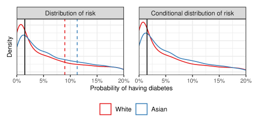
Drawing on recommendations from the United States Preventative Screening Task Force, Aggarwal et al. (2022) suggest screening patients with at least a 1.5% risk of diabetes, irrespective of race. We depict this risk threshold by the solid black vertical line in the plot. Based on that recommendation, 81% of Asian Americans and 69% of White Americans are to the right of the threshold and should be screened—violating demographic parity. If, hypothetically, we were to raise the screening threshold to 2.2% for Asian Americans and lower the threshold to 1% for White Americans, 75% of people in both groups would be screened, satisfying demographic parity.171717Corbett-Davies et al. (2017) show that group-specific threshold policies are utility-maximizing under the constraint of satisfying various notions of classification parity, including demographic parity and equality of false positive rates. The cost of doing so, however, would be failing to screen some Asian Americans who have a relatively high risk of diabetes, and subjecting some relatively low-risk White Americans to a procedure that is medically inadvisable given their low likelihood of having diabetes. In an effort to satisfy demographic parity, we would have harmed members from both groups.
This example illustrates a similar incompatibility between threshold policies and equalized false positive rates. In our setting, the false positive rate for a group is the screening rate among those in the group who do not in reality have diabetes. To visualize the race-specific false positive rates, the right-hand panel of Figure 2 shows the distribution of diabetes risk among those individuals who do not have diabetes. (Because the overall prevalence of diabetes is low, the conditional distribution displayed in the right-hand panel is nearly identical to the unconditional distribution displayed in the left-hand panel.) The false positive rate for each group is the proportion of people in the group falling to the right of the 1.5% screening threshold. In this case, the false positive rate is 79% for Asian Americans and 67% for White Americans—violating equalized false positive rates. As before, we could alter the screening guidelines to equalize false positive rates, but doing so requires deviating from our threshold policy, in which case we would end up screening some individuals who are relatively low-risk and not screening others who are relatively high-risk.
In this example, the incompatibility between threshold policies and classification parity stems from the fact that the risk distributions differ across groups. This general phenomenon is known as the problem of inframarginality in the economics and statistics literature, and has long been known to plague tests of discrimination in human decisions (Simoiu et al., 2017; Ayres, 2002; Galster, 1993; Carr and Megbolugbe, 1993; Knowles et al., 2001; Engel and Tillyer, 2008; Anwar and Fang, 2006; Pierson et al., 2018). Common legal and economic understandings of fairness are concerned with what happens at the margin (e.g., whether the same standard is applied to all individuals)—a point we return to in Section 5. What happens at the margin also determines whether decisions maximize social welfare, with the optimal threshold set at the point where the marginal benefits equal marginal costs. However, popular error metrics assess behavior away from the margin, hence they are called infra-marginal statistics. As a result, when risk distributions differ, standard error metrics are often poor proxies for individual equity or social well-being.
In general, we expect any two non-random subgroups of a population to differ on a variety of social and economic dimensions, which in turn is likely to yield risk distributions that differ across groups. As a result, as our running diabetes example shows, the optimal decision policy—which maximizes each patient’s own well-being—will likely violate various measures of classification parity. Thus, to the extent that formal measures of fairness are violated, that tells us more about the shapes of the risk distributions than about the quality of decisions or the utility delivered to members of any group. This intuition can be made precise, in the sense that for almost every risk distribution, the optimal decision policy violates the various notions of classification parity considered here.
The notion of almost every distribution that we use here was formalized by Christensen (1972), Hunt et al. (1992), Anderson and Zame (2001), and others (cf. Ott and Yorke, 2005, for a review). Suppose, for a moment, that combinations of covariates and outcomes take values in a finite set of size . Then the space of joint distributions on covariates and outcomes can be represented by the unit -simplex: . Since is a subset of an -dimensional hyperplane in , it inherits the usual Lebesgue measure on . In this finite-dimensional setting, almost every distribution means a subset of distributions that has full Lebesgue measure on the simplex. Given a property that holds for almost every distribution in this sense, that property holds almost surely under any probability distribution on the space of distributions that is described by a density on the simplex. We use a generalization of this basic idea that extends to infinite-dimensional spaces, allowing us to consider distributions with arbitrary support. (See the Appendix for further details.)
Theorem 9
Let be the optimal decision threshold, as in Eq. (9). If , then for almost every collection of group-specific risk distributions which have densities on , no utility-maximizing decision policy satisfies demographic parity or equalized false positive rates.
The proof of Theorem 9, which formalizes the informal discussion above, is given in Appendix F.6. At a high level, the constraints of classification parity are sensitive to even small perturbations in the underlying risk distributions. As a result, any particular collection of risk distributions is unlikely to satisfy the constraints. For simplicity, we have been considering settings in which the decision does not impact the outcome . However, this basic style of argument extends to causal settings, showing that threshold policies are almost surely, in the measure theoretic sense, incompatible with counterfactual predictive parity, counterfactual equalized odds, and conditional principal fairness—definitions of fairness that we consider in depth in Section 4, in the more complex setting of having a budget .
3.3 The Problem with Fairness through Unawareness
We now consider notions of fairness, both causal and non-causal, that aim to limit the effects of attributes on decisions. As above, we show the inherent incompatibility of these definitions with optimal decision making. We note, though, that while blinding can lead to suboptimal decisions—and, in some cases, harm marginalized groups—the legal, political, and social benefits of, for example, race-blind and gender-blind algorithms may outweigh their costs in certain instances (Cerdeña et al., 2020; Coots et al., 2023).
3.3.1 Blinding
A common starting point for designing an ostensibly fair algorithm is to exclude protected characteristics from the statistical model. This strategy ensures that decisions have no explicit dependence on group membership. For instance, in the case of estimating diabetes risk, one could use only BMI and age—rather than including race, as we did above. However, excluding race from models of diabetes risk can ultimately harm both White and Asian patients.
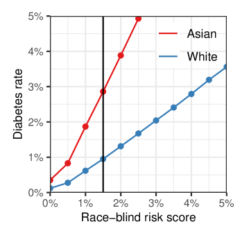
In Figure 3(a), we compare the actual diabetes rate to estimated diabetes risk resulting from the race-blind risk model. Aggarwal et al. (2022) showed that Asian patients have higher incidence of diabetes than White patients with comparable age and BMI. As a result, the race-blind model systematically underestimates risk for Asian patients and systematically overestimates risk for White individuals. In particular, applying a nominal 1.5% screening threshold under the race-blind model amounts to effectively applying a 1% screening threshold to White patients and a 3% screening threshold to Asian patients. Thus, by using race-blind risk scores, we subject relatively low-risk White patients to screening, and fail to screen Asian patients who have a relatively high risk for having diabetes. A race-aware model would ensure that nominal risk thresholds correspond to observed incidence rates across race groups.
This phenomenon—which we call miscalibration across subgroups—is not unique to diabetes screening. Consider, for instance, the case of pretrial recidivism predictions. Shortly after an individual is arrested in the United States, a judge must often determine conditions of release pending future court proceedings. In many jurisdictions across the country, these pretrial decisions are informed by statistical risk estimates of the likelihood the individual would be arrested or convicted of a future crime if released. After adjusting for factors such as criminal history, age, and substance use, women have been found to reoffend less often than men in many jurisdictions (Skeem et al., 2016; DeMichele et al., 2018). Consequently, gender-blind risk assessments are miscalibrated, meaning that they tend to overstate the recidivism risk of women and understate the recidivism risk of men.
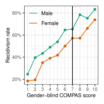
Figure 3(b) illustrates this point, plotting the observed recidivism rate for men and women in Broward County, Florida as a function of their gender-blind COMPAS risk scores—a commonly used risk assessment tool (Bao et al., 2021). In particular, women with a COMPAS score of seven recidivate about 55% of the time, whereas men with the same score recidivate about 65% of the time. Said differently, women with a score of seven recidivate approximately as often as men with a score of five, and this two-point differential persists across the range of scores. By acknowledging the predictive value of gender in this setting, one could create a decision rule that detains fewer people (particularly women) while achieving the same public safety benefits. Conversely, by ignoring this information and basing decisions solely on the gender-blind risk assessments, one would effectively be subjecting women to a more stringent risk standard—and potentially harsher penalties—than men.
As in the case of classification parity, one cannot typically remove protected attributes from the risk predictions without decreasing utility (cf. Manski et al., 2022); however, the reduction in utility is not always as large as one might expect (Coots et al., 2023). In concrete terms, in our running diabetes example, basing decisions on race-blind risk estimates necessarily means screening some patients who would have preferred not to be screened had they been given race-aware risk estimates, and, conversely, not screening some patients who would have preferred to be screened had they been given the more complete estimates. We state this result formally below.
Theorem 10
Suppose , where is the optimal decision threshold on the risk scale, as in Eq. (9). Let denote restriction to the unprotected covariates. Let denote the risk estimated using the blinded covariates. Suppose that and have densities on that are positive in a neighborhood of . Further suppose that there exists such that the conditional variance a.s., where is the risk estimated from the full set of covariates. Then no blind policy is utility-maximizing.
The proof of Theorem 10 is given in Appendix D. In short, when race, gender, or other protected traits add predictive value—a condition codified in our assumption that the conditional variance be greater than —excluding these attributes will in general decrease utility, both for individuals and in the aggregate.
Basing decisions on blinded risk scores can harm individuals and communities, for example by failing to flag relatively high-risk Asian patients for diabetes screening. But it is also important to consider potential harms stemming from the use of race- and gender-specific risk tools. In medicine, for instance, one might worry that race-specific risk assessments could encourage doctors and the public-at-large to advance spurious and pernicious arguments about inherent differences between race groups. In reality, the differences in diabetes risk we see are likely due to a complex mix of factors, both environmental and genetic, and should not be misinterpreted as indicating any causal effects of race. Indeed, even “race” itself is a thorny, socially influenced, concept, that elides easy definition. Similarly, the use of gender-specific recidivism estimates could reduce trust in the criminal justice system, giving the impression that individuals are held to different standards based on their gender. (Though, as we have seen above, blinded risk assessments can likewise—and perhaps more persuasively—be said to subject individuals to different standards based on their race and gender.) In some circumstances, race- and gender-specific risk estimates are even prohibited by law—a topic we return to in Section 5.1. For these reasons, risk assessments in medicine, criminal justice, and beyond have generally avoided using race, gender, and other sensitive demographic attributes. Ultimately, when constructing risk assessment tools, it is important to acknowledge and carefully balance both the costs and benefits of blinding in any given circumstance.
3.3.2 Counterfactual and Path-Specific Fairness
As discussed in Section 2, counterfactual and path-specific fairness are generalizations of simple blinding that attempt to account for both the direct and indirect effects of protected attributes on decisions. Because the constraints are more stringent, the resulting decrease in utility is proportionally greater. In particular, in some common settings, path-specific fairness with constrains decisions so severely that the only allowable policies are constant (i.e., for all ). For instance, in our running admissions example, path-specific fairness requires admitting all applicants with the same probability, irrespective of academic preparation or group membership.
To build intuition for this result, we sketch the argument for a finite covariate space . Given a policy that satisfies path-specific fairness, select . By the definition of path-specific fairness, for any ,
| (10) | ||||
That is, the probability of an individual with covariates receiving a positive decision must be the average probability of the individuals with covariates in group receiving a positive decision, weighted by the probability that an individual with covariates in the real world would have covariates counterfactually.
Next, we suppose that there exists an such that for all . In this case, because for all , Eq. (10) shows that in fact for all .
Now, let be arbitrary. Again, by the definition of path-specific fairness, we have that
where we use in the third equality the fact for all , and in the final equality the fact that is supported on .
Theorem 11 formalizes and extends this argument to more general settings, where is not necessarily positive for all . The proof of Theorem 11 is in the Appendix, along with extensions to continuous covariate spaces and a more complete characterization of -fair policies for finite .
Theorem 11
Suppose is finite and for all . Suppose is a random variable such that:
-
1.
for all ,
-
2.
for all such that , , and such that .
Then, for any -fair policy , with , there exists a function such that , i.e., is constant across individuals having the same value of .
The first condition of Theorem 11 holds for any reduced set of covariates that is not causally affected by changes in (e.g., is not a descendant of ). The second condition requires that among individuals with covariates , a positive fraction have covariates in a counterfactual world in which they belonged to another group . Because is the same in the real and counterfactual worlds—since is unaffected by , by the first condition—we only consider such that in the second condition.
In our admissions example, this result shows that, under mild conditions, causally-fair policies require admitting all applicants with equal probability. In particular, suppose that among students with a given test score, a positive fraction achieve any other test score in the counterfactual world in which their race is altered—as, for instance, we might expect if the individual-level causal effects are drawn from an (appropriately discretized) normal distribution. In this case, the empty set of reduced covariates—formally encoded by setting to a constant function—satisfies the conditions of Theorem 11. The theorem then implies that under any -fair policy, every applicant is admitted with equal probability. (We motivated our admissions example by assuming that only a fraction of applicants could be admitted; however, Theorem 11 holds irrespective of the budget, and, in particular, when , and so we discuss this result together with our others on unconstrained decision making as a natural extension of blinding.)
Even when decisions are not perfectly uniform lotteries, Theorem 11 suggests that enforcing -fairness can lead to unexpected outcomes. For instance, suppose we modify our admissions example to additionally include age as a covariate that is causally unconnected to race—as some past work has done. In that case, -fair policies would admit students based on their age alone, irrespective of test score or race. Although in some cases such restrictive policies might be desirable, this strong structural constraint implied by -fairness appears to be a largely unintended consequence of the mathematical formalism.
The conditions of Theorem 11 are relatively mild, but do not hold in every setting. Suppose that in our admissions example it were the case that for some constant —that is, suppose the effect of intervening on race is a constant change to an applicant’s test score. Then the second condition of Theorem 11 would no longer hold for a constant . Indeed, any multiple-threshold policy in which would be -fair. In practice, though, such deterministic counterfactuals would seem to be the exception rather than the rule. For example, it seems reasonable to expect that test scores would depend on race in complex ways that induce considerable heterogeneity. Lastly, we note that in some variants of path-specific fairness (e.g., Zhang and Bareinboim, 2018; Nabi and Shpitser, 2018), in which case Theorem 11 does not apply. Although, in that case, path-specific fairness is still typically incompatible with optimal decision-making, as shown in Theorem 17.
4 Equitable Decisions in the Presence of Externalities
We have thus far considered cases where there is largely agreement on the utility of different decision policies. In that setting, we showed that maximizing utility is at odds with various mathematical formalizations of fairness. We further argued that these results illustrate weaknesses in the formalizations themselves, since deviating from utility-maximizing polices in that setting can harm both individuals and groups—as seen in our diabetes screening example.
Agreement on the utility, however, is perhaps the exception rather than the rule. One could indeed argue that the value of mathematical formalizations of fairness is their ability to arbitrate between competing definitions of utility. Here we critically examine that perspective. We show, in analog to our previous results, that even when it is unclear how to balance competing priorities, enforcing existing fairness constraints typically leads to worse outcomes on each dimension. For instance, in our running college admissions example, policies constrained to satisfy various fairness constraints will typically require admitting a student body that is both less academically prepared and less diverse, relative to alternative policies that violate these mathematical fairness definitions.
We start, in Section 4.1, by examining our college admissions example in detail, illustrating in geometric terms how existing fairness definitions can lead to problematic admissions policies. Then, in Section 4.2, we develop our formal theory of equitable decision making in the presence of externalities. The mathematics necessary to establish our key results are significantly deeper than what we have needed thus far, but our high-level message is the same: enforcing several formal notions of fairness leads to policies that can paradoxically harm the very groups that they were designed to protect.
4.1 The Geometry of Fair Decision Making
To build intuition about the limitations of popular definitions of fairness, we return to our running example on college admissions. In that setting, we imagine an admissions committee debating the merits of different admissions policies. In particular, we imagine disagreement within the committee over how best to balance two competing objectives: academic preparation (operationalized, e.g., in terms of the high school grades and standardized test scores of admitted students) and class diversity (e.g., the number of admitted applicants from marginalized groups).
We assume that our hypothetical committee members all agree that more (total) academic preparedness and more class diversity are better. Thus, in the absence of any resource constraints (with , as is approximated in some online courses), the university could admit all applicants, maximizing both the number of admitted students from marginalized groups and also the total academic preparedness of the admitted class. But given limits on the number of students who can be admitted (i.e., ), one must make difficult choices on whom to admit, with reasonable and expected disagreement on how much to trade one dimension for another. The trade-offs in decision making are most acute when the budget , and for this reason we focus here on that case.
In light of these trade-offs, one might turn to the myriad formal fairness criteria we have discussed to ensure admissions decisions are equitable. Many of the fairness definitions we consider make reference to a distinguished outcome . In our example, we can imagine this outcome corresponds to college degree attainment, an ex post measure of academic preparedness. In the case of causal fairness definitions, we could take to mean degree attainment if the student were admitted, and to be degree attainment if the student were not admitted, with the understanding that a student who is not admitted could potentially attend and graduate from another university. For example, satisfying counterfactual predictive parity requires that among rejected applicants, the proportion who would have attained a college degree, had they been accepted, is equal across race groups. In these cases, we imagine academic preparedness is some student-level measure that connects observables —upon which the committee must make their admissions decisions—to (potential) outcomes . For example, the “academic index” might be a prediction of given based on historical data, or, more generally, could encode committee preferences for both academic preparation and participation in extracurricular activities, among other factors.
The key point of our informal discussion thus far is that we assume committee members would like to enact an admissions policy that balances two competing objectives. First, they would like a policy that leads to large , i.e., they would like to be big, where is some quantity that may, for example, encode academic preparedness and other preferences. Second, the committee would like large diversity, i.e., they would like to be big, where corresponds to some target group of interest. All committee members would like more of each dimension, but, given the budget constraint, it is in general impossible to maximize both dimensions simultaneously, leading to the inherent trade-offs we consider in this section.
We now explore the consequences of imposing additional fairness constraints on our college admissions example, as given by the causal DAG in Figure 1, via a simulation study of one million hypothetical applicants, for one quarter of whom () seats are allocated. In particular, in the hypothetical pool of applicants we consider, applicants in the target race group have, on average, fewer educational opportunities than those applicants in group , which leads to lower average academic preparedness, as well as lower average test scores. We define the “academic index” of applicants to be the estimated probability that an applicant will graduate if admitted, based on their observed test score and race. See Appendix C for additional details, including the specific structural equations we use in the simulation.
Each of the panels in Figure 4 illustrates the geometry of fairness constraints for five different formal notions of fairness described in Section 2: counterfactual fairness, path-specific fairness, principal fairness, counterfactual equalized odds, and counterfactual predictive parity. The vertical axes of each panel correspond to aggregate academic index and the horizontal axes to the number of admitted applicants from the target group. The purple lines trace out the boundary of the set of feasible policies, with points on or below the curves achievable by policies that adhere to the budget constraint. Policies lying strictly below the purple curves (or, similarly, on the dashed segments of the purple curves) are “Pareto dominated,” meaning that one can find feasible alternatives that are larger on both of the depicted axes (i.e., academic index and diversity). Since we have assumed committee members prefer higher values on each dimension, their effective choice set consists of those policies on the solid purple segments—the “Pareto frontier.” Committee members may still disagree over which policy on the frontier to adopt. But for any policy not on the frontier, there is a feasible policy above and to the right of it, which is thus preferred by every member of the committee.

Finally, the shaded regions indicate the set of feasible policies constrained to satisfy each of the fairness definitions. (In Appendix B, we show that these feasibility regions can be computed by solving a series of linear programs.) In each case, the constrained regions do not intersect the Pareto frontier, and so there is an alternative, unconstrained feasible policy that simultaneously achieves more student-body diversity and an overall higher academic index. For example, in the case of policies satisfying counterfactual or path-specific fairness, shown in the upper left panel, the set of feasible policies lie on a single line segment. That structure follows from Theorem 11, since the only policies satisfying either of these notions of fairness in our setting are ones that admit all students with a constant probability, irrespective of their covariates. While not as extreme, the other fairness definitions similarly restrict the space of feasible policies in severe ways, as shown in the remaining panels. These results illustrate that constraining decision-making algorithms to satisfy popular definitions of fairness can have unintended consequences, and may even harm the very groups they were ostensibly designed to help.
Our discussion in this section aimed to highlight the geometry of “fair” decision policies and their consequences in the context of a simple motivating example. We next show that these qualitative findings are guaranteed to hold much more generally.
4.2 A Formal Theory of Fairness in the Presence of Externalities
Our simulation above showed that policies satisfying one of the mentioned fairness definitions are suboptimal, in the sense that they constrain one to a portion of the feasible region in which policies could be improved along both dimensions of interest. As was the case in the absence of trade-offs in Section 3.2, the phenomenon occurring in our simulation is true much more generally. To understand why, we begin by isolating and formalizing the relevant mathematical properties of our example. To generalize our setting in Section 3, we consider arbitrary utility functions of the form . As before, for a function and decision policy , we write to denote the expected utility of decision policy under the utility . An important constraint on the admissions committee was the fact that their admissions decisions could not, in expectation, exceed the budget.
Definition 12
For a budget , we say a decision policy is feasible if .
A key feature of the college admissions example is that despite some level of uncertainty regarding the “true” utility—i.e., exactly how to trade off between its objectives—the committee knows what its objectives are: to increase the academic index and diversity of the incoming class. One way to encode this kind of uncertainty is to consider a set consisting of all “reasonable” ways of trading off between the objectives. While the utilities need not be the same, they should be consistent, in the sense that conditional on an applicant’s group membership, all of the utilities should “agree” that a higher academic index is better.
Definition 13
We say that a set of utilities is consistent modulo if, for any :
-
1.
For any , ;
-
2.
For any and such that , if and only if .
A second relevant feature of the admissions problem is that certain policies were strictly better from the admissions committee’s perspective, despite their uncertainty about the exact form of their utility. The notion that one policy is better than another regardless of the exact form of the utility is formalized by Pareto dominance.
Definition 14
Suppose is a collection of utility functions. A decision policy is Pareto dominated if there exists a feasible alternative such that for all , and there exists such that . A policy is strongly Pareto dominated if there exists a feasible alternative such that for all . A policy is Pareto efficient if it is feasible and not Pareto dominated, and the Pareto frontier is the set of Pareto efficient policies.
As discussed above and in Section 3.1, in the absence of trade-offs, optimal decision policies take the simple form of threshold policies. The existence of trade-offs broadens the range of forms a Pareto efficient policy can take. Even so, for consistent collections of utilities, the Pareto efficient policies take a closely related form.
Proposition 15
Suppose is a set of utilities that is consistent modulo . Then any Pareto efficient decision policy is a multiple-threshold policy. That is, for any , there exist group-specific constants such that, a.s.:
| (11) |
The proof of Proposition 15 is in the Appendix.181818In the statement of the proposition, we do not specify what happens at the thresholds themselves, as one can typically ignore the exact manner in which decisions are made at the threshold. Specifically, given a multiple-threshold policy , we can construct a standardized multiple-threshold policy that is constant within group at the threshold (i.e., when ), and for which: (1) ; and (2) . In our running example, this means we can standardize multiple-threshold policies so that applicants at the threshold are admitted with the same group-specific probability.
4.2.1 Fairness definitions with many constraints
All of the definitions we study in this section prominently feature causal quantities, but the important quality driving our analysis in this section is that each definition imposes many constraints. For instance, counterfactual equalized odds requires that
for every outcome .
Theorem 17 shows that for almost every joint distribution of , , and such that has a density, any feasible decision policy satisfying counterfactual equalized odds or conditional principal fairness is Pareto dominated. Similarly, for almost every joint distribution of and , we show that feasible policies satisfying path-specific fairness—including counterfactual fairness—are Pareto dominated. (The analogous statements for counterfactual predictive parity, equalized false positive rates, and demographic parity are not true; we return to this point in Section 4.2.2.) That is, we show that, for a typical joint distribution, any feasible policy satisfying the fairness definitions enumerated above cannot have the form of a multiple-threshold policy. To prove this result, we make relatively mild restrictions on the set of distributions and utilities we consider to exclude degenerate cases, as formalized by Definition 16.
Definition 16
Let be a collection of functions from to for some set . We say that a distribution of on is -fine if has a density for all .
In particular, -fineness ensures that the distribution of has a density. In the absence of -fineness, corner cases can arise in which an especially large number of policies may be Pareto efficient, in particular when has large atoms and can be used to predict the potential outcomes and even after conditioning on . See Proposition 72 in the Appendix for details.
Theorem 17
Suppose is a set of utilities consistent modulo . Further suppose that for all there exist a -fine distribution of and a utility such that , where . Then,
-
•
For almost every -fine distribution of and , any feasible decision policy satisfying counterfactual equalized odds is strongly Pareto dominated.
-
•
If and there exists a -fine distribution of such that for all and , where , then, for almost every -fine joint distribution of , , and , any feasible decision policy satisfying conditional principal fairness is strongly Pareto dominated.
-
•
If and there exists a -fine distribution of such that for all and some distinct , then, for almost every -fine joint distributions of and the counterfactuals , any feasible decision policy satisfying path-specific fairness is strongly Pareto dominated.191919Here, and is the set of for , i.e., component-wise application of to elements of . In other words, the requirement is that the joint distribution of the has a density.
The proof of Theorem 17 is given in the Appendix. At a high level, the proof proceeds in three steps, which we outline below using the example of counterfactual equalized odds. First, we show that for almost every fixed -fine joint distribution of and there is at most one policy satisfying counterfactual equalized odds that is not strongly Pareto dominated. To see why, note that for any specific , since counterfactual equalized odds requires that , setting the threshold for one group determines the thresholds for all the others; the budget constraint then can be used to fix the threshold for the original group. Second, we construct a “slice” around such that for any distribution in the slice, is still the only policy that can potentially lie on the Pareto frontier while satisfying counterfactual equalized odds. We create the slice by strategically perturbing only where , for some . This perturbation moves mass from one side of the thresholds of to the other. Due to inframarginality, this perturbation typically breaks the balance requirement for almost every in the slice. Finally, we appeal to the notion of prevalence to stitch the slices together, showing that for almost every distribution, any policy satisfying counterfactual equalized odds is strongly Pareto dominated. Analogous versions of this general argument apply to the cases of conditional principal fairness and path-specific fairness.202020This argument does not depend in an essential way on the definitions being causal. In Corollary 70 in the Appendix, we show an analogous result for the non-counterfactual version of equalized odds. We note that the conditions of Theorem 17 are sufficient, rather than necessary, meaning that the conclusion of the theorem may—and, indeed, we expect will—hold even in some cases where the conditions are not satisfied. In particular, we note that this proof technique prevents the conditions of Theorem 17 from holding when factors through and, in particular, when . Although, when , Theorem 11 shows that under slightly different conditions, a much stronger result holds.
To bring our discussion full circle, we now map Theorem 17 onto the motivation offered in Section 4.1. Recall that the admissions committee knew that given the opportunity, it preferred policies that increased both the overall academic index of its admitted class, and policies that resulted in more students being admitted from the target group. In other words, we imagine that members of the admissions committee have utilities of the form212121Strictly speaking, we are saying that members of the admissions committee, rather than having an aggregate utility—which, as we have considered so far, has the form —has a utility on aggregate outcomes.
| (12) |
where, as above, denotes the academic index of an applicant with covariates , and increases in both coordinates. Corollary 18 establishes the inherent incompatibility of such preferences with the formal fairness criteria we have been considering.
Corollary 18
Consider a utility of the form given in Eq. (12), where is monotonically increasing in both coordinates and . Then, under the same hypotheses as in Theorem 17,222222The full statement is given in Appendix F.7. for almost every joint distribution, no utility-maximizing decision-policy satisfies counterfactual equalized odds, conditional principal fairness, or path-specific fairness.
Lastly, while, in general, one’s decision policy can depend only on the covariates known at the time of the decision, in some cases, the restriction that be a function of alone may be too restrictive; the connection between an individual having covariates and our utility may depend also on the relationship between and . For instance, in the admissions example, the admissions committee may value high test scores and extracurriculars not, e.g., as per se measures of academic merit, but rather instrumentally insofar as they are connected to whether an applicant will eventually graduate. However, allowing to depend on both and greatly complicates the underlying geometry of the problem. Proving Theorem 17 in this more general setting remains an open problem. However, intuition from finite-dimensions—where more powerful measure-theoretic tools are available—suggests that the result remains true in the more general setting. For example, Proposition 19 presents a version of this result over a natural, finite-dimensional family of distributions.
Proposition 19
Suppose , and consider the family of utility functions of the form
indexed by , where . For almost every , if the conditional distributions of given are beta distributed with
then any policy satisfying counterfactual equalized odds is strongly Pareto dominated.
4.2.2 Fairness definitions with few constraints
We conclude this analysis by considering equalized false positive rates, demographic parity, and counterfactual predictive parity. These fairness notions are less demanding than the notions considered above, in that they introduce only “one” additional constraint, e.g., that , in the case of counterfactual predictive parity. Since the budget introduces a second constraint, and the form of a multiple-threshold policy allows for a degree of freedom in each group, the number of constraints and the number of degrees of freedom are equal—as opposed to the causal fairness definitions covered by Theorem 17, in which the constraints outnumber the degrees of freedom. As such, it is possible in some instances to have a policy on the Pareto frontier that satisfies these conditions; though see Section 5.3 for discussion about why such policies are still often at odds with broader goals.
However, it is not always possible to find a point on the Pareto frontier satisfying these definitions. In Proposition 20, we show that counterfactual predictive parity cannot lie on the Pareto frontier in some common cases, including our example of college admissions. In that setting, when the target group has lower average graduation rates—a pattern that often motivates efforts to actively increase diversity—decision policies constrained to satisfy counterfactual predictive parity are Pareto dominated. The proof of the proposition is in Appendix H.3.
Proposition 20
Suppose , and consider the family of utility functions of the form
indexed by , where . Suppose the conditional distributions of given are beta distributed, i.e.,
with and .232323Here we parameterize the beta distribution in terms of its mean and sample size . In terms of the common, alternative - parameterization, and . Then any policy satisfying counterfactual predictive parity is strongly Pareto dominated.
5 A Path Forward
We have thus far worked to clarify some of the statistical limitations of existing mathematical definitions of fairness. We have argued that in many cases of interest, these definitions can ultimately do more harm than good, hurting even those individuals that these notions of fairness were ostensibly designed to help.
We end on a more optimistic note, charting out a potential path toward designing more equitable algorithms. To do so, we start, in Section 5.1 by reviewing conceptions of discrimination in law and economics, and, in particular, we contrast process-oriented and outcome-oriented notions of fairness. Whereas the computer science literature is dominated by process-oriented, deontological definitions of fairness, we see more promise in adopting an outcome-oriented, consequentialist approach represented by the utilitarian analysis we have described above. In Section 5.2, we enumerate and discuss four issues that we feel are critical in developing equitable algorithms: (1) balancing inherent trade-offs in decision problems; (2) assessing calibration; (3) selecting the inputs and targets of prediction; and (4) designing data collection strategies. Finally, in Section 5.3, we illustrate how to grapple with these considerations in a case study of complex medical care, motivated by work from Obermeyer et al. (2019).
5.1 Competing Notions of Ethical Decision Making: Process vs. Outcomes
There are many distinct but related understandings of ethical decision making in law, economics, philosophy, and beyond. One key dimension on which we organize these notions is the extent to which they consider the process through which decisions are made versus the outcomes that those decisions render.
The dominant legal doctrine of discrimination in the United States treats explicit race- and gender-based decisions with heightened scrutiny. The Equal Protection Clause of the U.S. Constitution’s Fourteenth Amendment restricts government agencies from adopting policies that explicitly reference legally protected categories, and myriad federal and state disparate treatment statutes similarly constrain a variety of private actors. Conversely, policies that do not explicitly consider legally protected traits—or obvious proxies—are generally deemed not to violate disparate treatment principles. Formally, it is lawful to use legally protected attributes in a limited way to further a compelling government interest, but, in practice, such exceptions are few and far between. Until recently, the prime example of a race-conscious policy passing legal muster was affirmative action in college admissions (Fisher v. University of Texas, 2016). However, in 2023, the U.S. Supreme Court barred the explicit consideration of race in admissions decisions (SFFA v. Harvard, 2023).
Disparate treatment doctrine has evolved over time, and reflects ongoing debates about the role of classification (use of protected traits, a process-oriented, deontological notion) versus subordination (subjugation of disadvantaged groups, an outcome-oriented notion) in discrimination cases (Fiss, 1976). Some legal scholars have argued that courts, even when formally applying anti-classification criteria, are often sympathetic to the potential effects of judgments on social stratification, indicating tacit concern for anti-subordination (Colker, 1986; Balkin and Siegel, 2003; Siegel, 2003). Others, though, have noted that such judicial support for anti-subordination appears to be waning (Nurse, 2014). At a high level, we thus view modern disparate treatment law as primarily interested in process over outcomes, though these debates illustrate that the two concepts cannot be perfectly separated.
In contrast to process-oriented disparate treatment principles, the economics literature distinguishes between two outcome-focused, consequentialist rationales for explicitly considering race, gender, and other protected traits: taste-based and statistical. With taste-based discrimination (Becker, 1957), decision makers act as if they have a preference or “taste” for bias, sacrificing profit to avoid certain transactions. This includes, for example, an employer who forfeits financial gain by failing to hire exceptionally qualified minority applicants. But, in contrast to legal reasoning, the economic argument against taste-based discrimination is not that decisions are based on race per se, but rather because consideration of race leads to worse outcomes: a loss of profit. With statistical discrimination (Arrow, 1973; Phelps, 1972), decision makers explicitly consider protected attributes in order to optimally achieve some non-prejudicial goal. For example, profit-maximizing auto insurers may charge a premium to male drivers to account for gender differences in accident rates. Despite their differing outcome-based justifications, both taste-based and statistical discrimination are often considered legally problematic as they explicitly consider race, in violation of disparate treatment laws.242424In the case of auto insurance specifically, some states (including California, Hawaii, Massachusetts, Maine, Michigan, North Carolina, and Pennsylvania)—though not all—have barred the use of gender in pricing policies.
As the above insurance example and our running diabetes example illustrate, one might consider it acceptable to base decisions in part on legally protected traits when doing so leads to good outcomes. Conversely, whereas process-oriented disparate treatment principles generally deem race-blind policies acceptable, one might declare such blind policies problematic if they lead to bad outcomes. Indeed, under the statutory disparate impact standard, a practice may be deemed discriminatory if it has an unjustified adverse effect on legally protected groups, even in the absence of explicit categorization (Barocas and Selbst, 2016).252525The legal doctrine of disparate impact stems largely from federal statutes, not constitutional law, and applies only in certain contexts, such as employment (via Title VII of the 1964 Civil Rights Act) and housing (via the Fair Housing Act of 1968). Apart from federal statutes, some states have passed more expansive disparate impact laws, including Illinois and California. The distinction between statutory and constitutional rules is particularly relevant here, as there is debate among scholars over whether disparate impact laws violate the Equal Protection Clause and are thus unconstitutional (Primus, 2003). There is also debate over whether disparate impact law is motivated primarily by an interest in banning bad outcomes, or seeks to provide an alternative pathway for ferreting out bad intent, when actors may mask animus with race-neutral policies (Watson v. Fort Worth, 1988). But, regardless of its underlying justification, disparate impact law is formally focused on outcomes, not intent or classification, and so we view it as an outcomes-focused principle. The disparate impact doctrine was formalized in Griggs v. Duke Power Co., a 1971 U.S. Supreme Court case. In 1955, the Duke Power Company mandated that employees have a high school diploma to be considered for promotion, which, in practice, severely limited the eligibility of Black employees. The Court found that this facially race-neutral requirement had little relation to job performance, and accordingly deemed it to have an unjustified—and illegal—disparate impact. The Court noted that the employer’s motivation for instituting the policy was irrelevant to its decision; even if enacted without discriminatory purpose, the policy was deemed discriminatory in its effects and hence illegal. However, disparate impact law does not prohibit all group differences produced by a policy—the law only prohibits unjustified disparities. For example, if, hypothetically, the high-school diploma requirement in Griggs were shown to be necessary for job success, the resulting disparities would be legal.
On the spectrum from process- to outcome-based understandings of discrimination, we view the formal, axiomatic fairness definitions described in Section 2 as reflecting a largely process-based orientation. Blinding and its more stringent causal variants—counterfactual fairness and path-specific fairness—can be viewed as descendants of disparate treatment considerations, as they seek to remove the effects of race and other protected attributes on decisions. The remaining definitions—for example, those that aim to equalize error rates across groups—do explicitly reference an outcome , but they do so in a way that seems largely disconnected from the consequences one might naturally consider. As we have argued, whether error rates are equal across groups has more to do with the structure of group-specific risk distributions than with whether decisions lead to good or bad outcomes for group members. For example, in our college admissions example, enforcing various formal notions of fairness would, in theory, typically lead to student bodies that are both less diverse and less academically prepared than those resulting from feasible alternatives not constrained to satisfy these notions.
One might, on principle, favor certain process-based understandings of discrimination over outcome-based notions. One might even adopt a meta-consequentialist position, and argue that procedural considerations (e.g., ensuring medical decisions are blind to race) engender trust and in turn bring about better downstream outcomes. In many cases, though, the ethical underpinnings of popular mathematical definitions of fairness have not been clearly articulated. Absent such justification, we advocate for an approach that more directly engages with the real-world costs and benefits of different decision policies, a perspective that we outline in more detail in the remaining sections.
5.2 Designing Equitable Algorithms
A key advantage of the dominant axiomatic approach to algorithmic fairness is that it can be readily applied across contexts, with little domain-specific knowledge. One can build automated tests to check whether any predictive algorithm satisfies various formal fairness desiderata, and even automatically modify algorithms to ensure that they do satisfy a specific fairness criterion (e.g., Cotter et al., 2019; Weerts et al., 2023). But, as we have argued, this approach is often at odds with improving well-being, including for disadvantaged groups. A particularly pernicious risk of automated, axiomatic approaches is that they can make invisible the cost to well-being: automatically constraining algorithms to be “fair” can lead one to overlook unconstrained alternatives that are clearly preferable. We have instead called for a more careful analysis of the consequences, good and bad, of different decision policies, selecting the appropriate course of action based on the specific context. This is admittedly hard to do—and does not easily scale—but there are general principles that we believe are helpful to keep in mind when navigating this terrain. Below we enumerate and discuss four of them.
5.2.1 Contending with inherent trade-offs
There are inherent trade-offs in many important decision problems. For instance, in our college admissions example, one must balance academic preparedness with student-body diversity. Although one cannot generally circumvent these trade-offs, we believe it is useful to explicitly enumerate the primary dimensions of interest and to acknowledge the trade-offs between them. In some cases, like our stylized admissions example, one might be able to explicitly calculate the Pareto frontier shown in Figure 4, in which case it often makes sense to focus on those policies lying on the frontier. In many cases, it won’t be possible to compute the frontier. Still, by listing and discussing trade-offs, even informally, one can reduce the risk of adopting clearly problematic policies, like those that typically result from uncritically constraining decisions to satisfy formal fairness criteria.
In this sense, designing equitable algorithms is akin to designing equitable policy writ large. One might accordingly adapt democratic mechanisms used to draft and enact legislation to algorithm design. For example, adopting such a policy-oriented perspective, Chohlas-Wood et al. (2023a) and Koenecke et al. (2023) surveyed a diverse sample of Americans to elicit preferences on how best to balance competing objectives in programs that algorithmically allocate government benefits.
5.2.2 Assessing Calibration
When designing or auditing a risk assessment algorithm, it is important to check whether predictions are calibrated, meaning that risk scores correspond to the same observed level of risk across groups. In general, the relationship between predictors and outcomes may plausibly differ across groups, leading to miscalibrated risk estimates—what Ayres (2002) calls the problem of subgroup validity. Figure 3 shows instances of risk scores for diabetes and recidivism that are miscalibrated across race and gender, respectively. For example, a nominal 1.5% diabetes risk—based on age and BMI—corresponds to an actual, observed diabetes rate of approximately 1% among White patients and 3% among Asian patients. Similarly, among individuals receiving a COMPAS risk score of 7—based on criminal history and related factors—about 55% of women recidivate, compared to 65% of men. These miscalibrated risk scores can result in inequitable decisions. For instance, a policy to screen patients with a nominal diabetes risk of 1.5% or above—in line with existing medical recommendations (Aggarwal et al., 2022)—would overscreen White patients and underscreen Asian patients, harming individuals in both groups.
Calibration can often be visually assessed by plotting predicted risk against average outcomes, as in Figure 6 (cf. Arrieta-Ibarra et al., 2022). For a simple, more quantitative, measure, we recommend regressing observed outcomes against risk estimates and group membership. A coefficient of approximately zero on group membership suggests risk estimates correspond to similar average outcomes across groups, with deviations from zero indicating the degree of miscalibration.
In practice, miscalibration can often be rectified by training group-specific risk models, or, roughly equivalently, including group membership in a single risk model fit across groups. For example, diabetes risk models that include race, and recidivism risk models that include gender, are approximately calibrated. The relatively new literature on multicalibration has introduced new computational techniques to ensure predictions are simultaneously calibrated across many different subgroups (Hébert-Johnson et al., 2018). Of course, including protected traits in risk models raises additional legal and ethical challenges. In some cases, it may be possible to reduce or eliminate miscalibration by incorporating additional, non-protected covariates. Regardless, we believe it is important to check the calibration of risk scores to make informed decisions about if and how to address any observed disparities.
Calibration is an important necessary condition to ensure risk estimates correspond to actually observable levels of risk across groups. But it is not sufficient. Indeed, even calibrated risk scores can encode and reinforce deeply discriminatory policies. To see this, imagine a bank that wants to discriminate against Black applicants. Further suppose that: (1) within ZIP code, White and Black applicants have similar default rates; and (2) Black applicants live in ZIP codes with relatively high default rates. Then the bank can surreptitiously discriminate against Black borrowers by basing estimates of default risk only on an applicant’s ZIP code, ignoring all other relevant information. Such scores would be calibrated (White and Black applicants with the same score would default equally often), and the bank could use these scores to justify denying loans to nearly all Black applicants. The bank, however, would be sacrificing profit by refusing loans to creditworthy Black applicants,262626These applicants are creditworthy in the sense that they would have been issued a loan had the bank used all the information it had available to determine their risk. and thus engaging in taste-based discrimination. This discriminatory lending strategy is indeed closely related to the historical (and illegal) practice of redlining, and illustrates the limitations of calibration as a measure of equity.

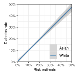
Figure 5 shows another example of calibrated scores masking disparities. In the left-hand panel, we plot in green the distribution of diabetes risk for Asian patients, as estimated from age, BMI, and race. In purple, we plot the distribution of estimated risk when age and BMI are imperfectly measured for Asian patients in the training data. Training the risk model on noisy features pushes risk estimates toward the mean. As a result, based on the noisy risk model, 97% of Asian patients are above the 1.5% screening threshold, compared to 81% of Asian patients under the more accurately estimated model—leading to more medically unnecessary screening under the noisy model. Importantly, however, the noisy model is still calibrated, as shown in the right-hand panel of Figure 5, where we compare risk scores for Asian patients estimated from the noisy predictors and risk scores for White patients estimated from the accurately estimated information. In theory, a malicious algorithm designer could generate such calibrated but inaccurate scores to intentionally harm Asian patients. In practice, this pattern could equally arise from negligence rather than malice. These examples illustrate the importance of considering all available data when constructing statistical risk estimates; assessments that either intentionally or inadvertently ignore predictive information may facilitate discriminatory decisions while satisfying calibration—though, as we discuss below, even this intuitive heuristic of “use all the data” has its limitations.
5.2.3 Selecting the target of prediction
In constructing algorithmic risk scores, a key ingredient is the target of prediction. In practice, though, there is often a mismatch between our true outcome of interest and the available data—an occurrence we call label bias (Zanger-Tishler et al., 2023). As with the other issues we discuss, there is typically no perfect solution to this problem, but there are ways to mitigate it.
For example, in pretrial risk assessment, we would often like to estimate the likelihood a defendant would commit a crime if released. But there are two key difficulties with this goal. First, though we might want to measure crime conducted by defendants awaiting trial, we typically only observe crime that results in a conviction or an arrest. These observable outcomes, however, are imperfect proxies for the underlying criminal act. Further, heavier policing in communities of color might lead to Black and Hispanic defendants being arrested, and later convicted, more often than White defendants who commit the same offense (Lum and Isaac, 2016). Poor outcome data might thus cause one to systematically underestimate the risk posed by White defendants. The second, related, issue is that our target of interest is a counterfactual outcome; it corresponds to what would have happened had a defendant been released. In reality, we only observe what actually happened conditional on the judge’s actual detention decision.
One way to reduce label bias in this case is to adjust the target of interest. For example, criminologists have found that arrests for violent crime—as opposed to drug crime—may suffer from less racial bias.272727D’Alessio and Stolzenberg (2003) find evidence that White offenders are even somewhat more likely than Black offenders to be arrested for certain categories of crime, including robbery, simple assault, and aggravated assault. Measurements of minor criminal activity, like drug offenses, are more problematic. For example, there is evidence that drug arrests in the United States are biased against Black and Hispanic individuals, with racial minorities who commit drug crimes substantially more likely to be arrested than White individuals who commit the same offenses (Ramchand et al., 2006). Although this pattern is well known, many existing risk assessment tools still consider arrests or convictions for any new criminal activity—including drug crimes—which may lead to biased estimates. As another example of label bias, auto insurance rates are determined in part by a driver’s record of receiving speeding tickets, but disparities in police enforcement mean that tickets are biased proxies of dangerous driving behavior (Cai et al., 2022b). In particular, Skeem and Lowenkamp (2016) note that the racial distribution of individuals arrested for violent offenses is in line with the racial distribution of offenders inferred from victim reports, and is also in line with self-reported offending data. In other cases, like lending, where one may seek to estimate default rates, the measured outcome (e.g., failure to pay) corresponds more closely to the event of interest. The problem of estimating counterfactuals can likewise be partially addressed in some applications. In the pretrial setting, Angwin et al. (2016) measure recidivism rates in the first two-year period during which a defendant is not incarcerated; this is not identical to the desired counterfactual outcome—since the initial detention may be criminogenic, for example—but it seems like a reasonable estimation strategy. Further, unaided human decisions often exhibit considerable randomness, a fact that can be exploited to facilitate statistical estimation of counterfactual outcomes (Jung et al., 2020b; Kleinberg et al., 2017a). More generally, a spate of recent work at the intersection of machine learning and causal inference (Mullainathan and Spiess, 2017; Hill, 2011; Jung et al., 2020c) offers hope for more gains in counterfactual estimation.
5.2.4 Collecting training data
A final issue we discuss is collecting suitable training data for risk assessment algorithms to mitigate the effects of sample bias. Ideally, one would train algorithms on data sets that are broadly representative of the populations on which they are ultimately applied—though there are subtleties to this heuristic that we describe below. While often challenging in practice, failure to train on representative data can lead to unintended, and potentially discriminatory, consequences. For example, Buolamwini and Gebru (2018) found that commercial facial analysis tools struggle to correctly classify the gender of dark-skinned individuals—and of dark-skinned women in particular—a disparity likely attributable to the relative dearth of dark-skinned faces in facial analysis data sets. Similarly, Koenecke et al. (2020) found that several popular automated speech recognition systems were significantly worse at transcribing Black speakers than White speakers, likely due to insufficient data from speakers of African American Vernacular English (AAVE), a variety of English spoken by many Black Americans.
The problems of non-representative data can be even more acute in the case of risk assessment algorithms, especially when the target of interest is a causal quantity. For instance, in our running college admissions example, we seek to estimate how a student would (counterfactually) perform if admitted. Historical data are typically the result of past, potentially biased, decisions, and so may not fully generalize. Imagine, for example, that predictions of college performance are informed by where an applicant went to high school, and that, historically, only applicants from certain high schools were accepted—and we consequently only see outcomes for students from those high schools. Then we would expect less accurate predictions for students from those absent high schools. In general, regression to the mean could attenuate estimates for high achieving students who differ from those previously accepted, potentially reinforcing existing admissions practices.
As a general heuristic, we believe it is advisable to train models on representative data, but, as Cai et al. (2022a) note, the optimal sampling strategy depends on the statistical structure of the problem and the group-specific costs of collecting data. Interestingly, the value of representative data collection strategies depends in part on the degree to which race, gender, and other protected attributes are predictive. In theory, if protected attributes are not predictive, one could build an accurate risk model using only examples from one particular group (e.g., White men). Given enough examples of White men, the model would learn the relationship between features and risk, which by our assumption would generalize to the entire population. This phenomenon highlights a tension in informal discussions of fairness, with some advocating both for representative training data and for the exclusion of protected attributes. However, representative data are often most important precisely when protected attributes add information, in which case their use is arguably more justified. Even if protected attributes are not predictive, representative data can still help in two additional ways. First, a representative sample ensures that the full support of features is present at training time, as it is possible that the distribution of features varies across groups, even if the connection between features and outcomes does not. We note, though, that one might have adequate support even without a representative sample in many real-world settings, particularly when models are trained on large data sets and the feature space is relatively low dimensional. Second, a representative sample can help with model validation, allowing one to assess the potential effects of group imbalance on model fit. In particular, without a representative sample, it can be difficult to determine whether a model trained on a single group generalizes to the entire population.
In many settings, one may be able to gather better training data with greater investment of time and money. For example, in our diabetes example one could aim to collect more complete medical records, a process that may be both costly and logistically difficult. In theory, this additional information may lead to welfare gains, and policymakers must accordingly evaluate the relative costs and benefits to all groups of exerting this extra effort when designing algorithms. Fortunately, in practice, there are often diminishing returns to information, with a relatively short list of key features providing most of the predictive power (Jung et al., 2020b), at least partially mitigating this concern.
As with the other issues we have discussed, there is no universal solution to data collection. It might, for example, simply be prohibitive in the short run to train models on the data set one would ideally like to use. Nevertheless, as in all situations, one must carefully weigh the potential costs and benefits of adopting a necessarily imperfect risk assessment algorithm relative to the other possible options. In particular, even an imperfect algorithm may in some circumstances be better than leaving decisions to similarly imperfect humans who have their own biases.
5.3 Case Study: An Algorithm to Allocate Limited Medical Resources
We conclude by illustrating the principles discussed above with a real-world example: an algorithm for referring patients into a “high-risk care management” program, previously considered by Obermeyer et al. (2019). The care management program more effectively aids patients with complex medical needs, in principle both improving outcomes for patients and reducing costs to the medical system for patients who are enrolled. But the program has limited capacity, which we formalize by assuming that only 2% of patients can be enrolled (i.e., we set ). For our analysis, we use the data released by Obermeyer et al.,282828Obermeyer et al. released a synthetic data set closely mirroring the real data set, available at: https://gitlab.com/labsysmed/dissecting-bias. In contrast to , which we adopt to better illustrate some of the statistical phenomena we discuss in this section, Obermeyer et al. use a budget of . which contain demographic variables, cost information, comorbidities, biomarker and medication details, and health outcomes for a population of approximately 43,000 White and 5,600 Black primary care patients at an academic hospital from 2013–2015.
As a first step toward identifying patients to enroll in the program, one could train a model predicting the healthcare resources a patient is likely to require over the next year. Sicker patients require more care and, consequently, incur greater healthcare costs. Thus, our initial approach is to predict how likely a patient is to be “high cost”—which we operationalize as being in the top decile of healthcare expenditures in a given year—based on the available information. (One of the main contributions of Obermeyer et al. (2019) is highlighting that healthcare costs is a problematic outcome due to label bias, a point we return to shortly.)
As discussed above, it is useful to assess the calibration of risk assessment algorithms across groups. In particular, while calibration across race is largely guaranteed if race is included as a predictor in the statistical model, race-blind models are often preferred, particularly in healthcare, in part to avoid perceptions of bias. As a result, we assess the calibration of a race-blind model trained on all available information except for race, shown in Figure 6. Unlike in the diabetes screening example considered in Section 3.2, the race-blind healthcare cost predictions are calibrated across race groups, meaning that risk estimates largely match observed costs across groups. It accordingly appears that race provides little marginal predictive power in this example, assuaging potential concerns with its omission.

We turn next to assessing the effects of applying formal fairness criteria to our enrollment decisions. Often, in healthcare contexts, a false negative—e.g., failing to screen for a disease when it is present—is more consequential than a false positive—e.g., screening for a disease when it is not present. For this reason, one might seek to ensure enrollment decisions are fair by mandating false negative rates be equal across race groups (e.g., Seyyed-Kalantari et al., 2021),292929The authors describe their metric of concern as the “false positive rate,” where the positive prediction is understood as a “no finding” label, e.g., not having a disease. In our example, we follow the more common convention that a “positive” classification is assigned to the rare event (i.e., being high cost), and so we call this metric the “false negative rate.” i.e., requiring that . In our example, equalizing false negative rates means that among patients who ultimately incur high medical costs (), the same proportion () are referred into the program across race groups ().

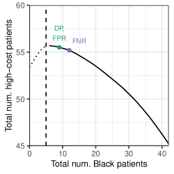
In our setting, approximately 1,000 patients can be referred into the care management program—2% of the roughly 50,000 patients in our data set. When we equalize false-negative rates, 747 of the enrolled patients ultimately incur high costs, and 113 enrolled patients are Black.303030Following Corbett-Davies et al. (2017), we equalize false-negative rates in a manner that maximizes the number of enrolled patients who ultimately incur high costs. However, an unconstrained decision rule (i.e., one that enrolls the patients most likely to incur high costs) enrolls both more high-cost patients (758) and more Black patients (205). In this example, we end up providing worse care to Black patients when we constrain our algorithm to satisfy the formal, mathematical fairness criterion.
Instead of applying such mathematical fairness criteria, we advocate for directly weighing the costs and benefits of different decision policies. In Figure 7(a), we show the Pareto frontier for our example, tracing out policies that optimally trade off the demographic composition of the enrolled population with the number of enrolled patients who in reality incur high costs. The green point corresponds to equalizing false negative rates, and is to the left of the dashed vertical line that corresponds to the unconstrained decision rule—visually illustrating how constraining our algorithm leads to fewer resources for Black patients. Also shown on the plot are points corresponding to demographic parity and equal false positive rates, both of which likewise lead to fewer resources for Black patients.313131As discussed in Section 4, with the exception of counterfactual predictive parity, all of the remaining fairness definitions given in Section 2 are known a priori to restrict one to enrollment policies that will lower both the number of Black patients enrolled as well as the number of truly high-cost patients enrolled.
The result in Figure 7(a) stems from the false negative rate for Black patients being lower than the false negative rate for White patients in the unconstrained algorithm—a pattern we expect since Black patients are more likely than White patients to incur high medical costs in our data. Equalizing false negative rates thus means raising the enrollment bar for Black patients and lowering the bar for White patients. In light of this example, one might argue for applying formal fairness criteria only when error rates for racial minorities are higher than for White individuals. Figure 7(b) repeats our analysis above for the subset of women between the ages of 25 and 34, a subpopulation in which Black patients have higher error rates than White patients. In this case, equalizing false positive rates or false negative rates, or enforcing demographic parity all result in more Black patients being admitted into the program. It is, however, unclear why one should adopt those particular error-rate equalizing policies over any other. The policies on the Pareto frontier (i.e., on the curve to the right of the dashed line) are all arguably reasonable to consider. It is admittedly difficult to determine which of these policies to adopt, but we believe it is best to confront this challenge head on, recognizing the hard trade-offs inherent to the problem.
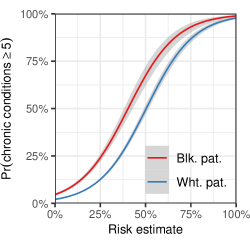

We conclude our case study by considering label bias, the primary concern identified by Obermeyer et al. (2019) in this context. As those authors noted, medical cost is a poor proxy for medical need, and so allocating healthcare resources to minimize anticipated costs can lead to severe disparities. Replicating an analysis by Obermeyer et al., Figure 8(a) shows that among patients with similar likelihood of incurring high-cost medical care, Black patients are considerably more likely than White patients to have complex medical needs, operationalized as having five or more active chronic conditions. This gap is likely a consequence of worse access to healthcare among Black patients, due to a mix of socioeconomic factors and discrimination. To the extent that care management programs aim to aid the sickest patients—as opposed to simply reducing costs—targeting resources based on anticipated costs can lead to inefficient and inequitable outcomes. Obermeyer et al. accordingly suggest switching the target of prediction from medical costs to health status.
It is possible to achieve further gains by recognizing resource allocation as an inherently causal problem. In particular, one may seek to enroll patients in the program in a manner that maximizes , where is the potential health outcome under the enrollment decision. To do so, we could prioritize patients by their estimated treatment effect , rather than an estimate of their future health status that ignores the causal effect of the program.323232In many analyses that do not explicitly grapple with the causal effects of interventions, the estimand is further corrupted by the fact that some patients are expected to be enrolled in the program. As a result, some of the sickest patients may not be prioritized for care, since their expected outcome already incorporates the fact that they would have been enrolled, leading to a prediction paradox. To avoid this situation, one could explicitly estimate and prioritize patients by , the potential outcome in the absence of care. In this case, however, the allocation decisions do not necessarily lead to the largest health gains, as the patients likely to be sickest in the absence of care are not typically the same as those likely to benefit the most from the program. A proper causal analysis is, in general, a complex topic requiring careful treatment beyond the scope of this article. Nonetheless, Figure 8(b) shows the distribution of , as estimated with a simple regression model. The plot suggests that there is considerable predictable heterogeneity in the extent to which enrollment in the care management program causally improves health. In particular, we find that the estimated treatment effect is only weakly correlated with the number of chronic conditions a patient currently exhibits (). Consequently, directly targeting resources to those most likely to benefit could yield large health improvements. Once the types of label bias we have discussed above have been identified, it may be possible to re-train predictive models to better align decision-making algorithms with policy goals.
6 Conclusion
From medicine to criminal justice, practitioners are increasingly turning to statistical risk assessments to help guide and improve human decisions. Algorithms can avoid many of the implicit and explicit biases of human decisions makers, but they can also exacerbate historical inequities if not developed with care. Policymakers, in response, have rightly demanded that these high-stakes decision systems be designed and audited to ensure outcomes are equitable. The research community has responded to the challenge, coalescing around several formal mathematical definitions of fairness. However, as we have aimed to articulate, these popular measures of fairness suffer from significant statistical limitations. Indeed, adopting these measures as algorithmic design principles can often harm the groups that these measures were designed to protect.
In contrast to the dominant axiomatic approach to algorithmic fairness, we advocate for a more consequentialist orientation (Nyarko et al., 2021; Chohlas-Wood et al., 2023a; Cai et al., 2022a; Liang et al., 2022). Most importantly, we stress the importance of grounding technical and policy discussions of fairness in terms of real-world quantities. For example, in the pretrial domain, one might consider a risk assessment’s short and long-term impacts on public safety and the size of the incarcerated population, as well as a tool’s alignment with principles of due process. In lending, one could similarly consider a risk assessment’s immediate and equilibrium effects on community development and the sustainability of a loan program. Formal mathematical measures of fairness only indirectly address such issues, and can inadvertently lead discussions astray. Of course, it is not always clear how best to quantify or to balance the relevant costs and benefits of proposed algorithmic interventions. In some cases, it may be possible to conduct randomized controlled trials; in other cases, the best one can do is hypothesize about an algorithm’s potential effects. Regardless, we believe a more explicit focus on consequences is necessary to make progress.
We further recommend decoupling the statistical problem of risk assessment from the policy problem of designing interventions. At their best, predictive algorithms estimate the likelihood of events under different scenarios; they cannot dictate policy. An algorithm might (correctly) infer that a defendant has a 20% chance of committing a violent crime if released, but that fact does not, in and of itself, determine a course of action. For example, detention is not the only alternative to release, as one could take any number of rehabilitative interventions (Barabas et al., 2018). Even if detention is deemed an appropriate intervention, one must still determine what threshold would appropriately balance public safety with the social and financial costs of detention. One might even decide that society’s goals are best achieved by setting different thresholds for different groups. For example, a policymaker might reason that, all else being equal, the social costs of detaining a single parent are higher than the social costs of detaining an individual without children, and thus decide to apply different thresholds to the two groups. When policymakers consider these options and others, we believe the primary role of a risk assessment tool is, as its name suggests, to estimate risk. This view, however, is at odds with requiring that algorithms satisfy popular fairness criteria. Such constrained algorithms typically do not reflect the best available estimates of risk, and thus implicitly conflate the statistical and policy problems.
Fair machine learning still has much left to accomplish and there are several important avenues of research that could benefit from new statistical and computational insights. From mitigating measurement error and sample bias, to understanding externalities and equilibrium effects, to eliciting and aggregating preferences to arbitrate between competing algorithms, there is much work to be done. But the benefits are equally large. When carefully designed and evaluated, statistical algorithms have the potential to dramatically improve both the efficacy and equity of consequential decisions. As these algorithms are increasingly deployed in all walks of life, it will become ever more important to ensure they are fair.
Acknowledgments and Disclosure of Funding
We thank Guillaume Basse, Sander Beckers, Hana Chockler, Alex Chohlas-Wood, Madison Coots, Avi Feller, Josh Grossman, Joe Halpern, Jennifer Hill, Aziz Huq, David Kent, Keren Ladin, Julian Nyarko, Emma Pierson, Ravi Sojitra, and Michael Zanger-Tishler for helpful conversations. This paper is based on work by Corbett-Davies and Goel (2018) and Nilforoshan et al. (2022). H.N was supported by a Stanford Knight-Hennessy Scholarship and an NSF Graduate Research Fellowship under Grant No. DGE-1656518. J.G was supported by a Stanford Knight-Hennessy Scholarship. R.S. was supported by the NSF Program on Fairness in AI in Collaboration with Amazon under the award “FAI: End-to-End Fairness for Algorithm-in-the-Loop Decision Making in the Public Sector,” no. IIS-2040898. S.G. was supported by a grant from the Harvard Data Science Initiative. Any opinions, findings, conclusions, or recommendations expressed in this material are those of the authors and do not necessarily reflect the views of the NSF or Amazon. Reproduction materials are available at https://github.com/jgaeb/measure-mismeasure.
Appendix A Path-specific Counterfactuals
Constructing policies which satisfy path-specific fairness requires computing path-specific counterfactual values of features. In Algorithm 1, we describe the formal construction of path-specific counterfactuals , for an arbitrary variable (or collection of variables) in the DAG. To generate a sample from the distribution of , we first sample values for the exogenous variables. Then, in the first loop, we traverse the DAG in topological order, setting to and iteratively computing values of the other nodes based on the structural equations in the usual fashion. In the second loop, we set to , and then iteratively compute values for each node. is computed using the structural equation at that node, with value for each of its parents that are connected to it along a path in , and the value for all its other parents. Finally, we set to .
Appendix B Constructing Causally Fair Policies
Our aim is to identify the feasible region of expected outcomes attainable via policies which are constructed to satisfy various causal fairness constraints.
First, consider the problem of finding decision policies that maximize expected utility, subject to satisfying a given definition of causal fairness, as well as the outcome and budget constraints. Specifically, letting denote the family of all decision policies that satisfy one of the causal fairness definitions listed above, a utility-maximizing policy is given by
| (13) | ||||
We prove that this optimization problem can be efficiently solved as a single linear program—in the case of counterfactual equalized odds, conditional principal fairness, counterfactual fairness, and path-specific fairness—or as a series of linear programs in the case of counterfactual predictive parity.
Theorem 21
Consider the optimization problem given in Eq. (13).
-
1.
If is the class of policies that satisfies counterfactual equalized odds or conditional principal fairness, and the distribution of is known and supported on a finite set of size , then a utility-maximizing policy constrained to lie in can be constructed via a linear program with variables and constraints.
-
2.
If is the class of policies that satisfies path-specific fairness (including counterfactual fairness), and the distribution of is known and supported on a finite set of size , then a utility-maximizing policy constrained to lie in can be constructed via a linear program with variables and constraints.
-
3.
Suppose is the class of policies that satisfies counterfactual predictive parity, that the distribution of is known and supported on a finite set of size , and that the optimization problem in Eq. (13) has a feasible solution. Further suppose is supported on points, and let be the unit -simplex. Then one can construct a set of linear programs , with each having variables and constraints, such that the solution to one of the LPs in is a utility-maximizing policy constrained to lie in .
Before moving on to the proof of Theorem 21, we note that since the constraints of the linear programs are convex, the feasible regions in Figure 4 can be determined by solving the convex feasibility problem where we impose the additional convex constraint that the expected outcomes—in our admissions example, the aggregate academic index and number of admitted applicants from the target group—lie within some distance of a given point. Performing a grid search over all points then determines the feasible regions.
Proof Let ; then, we seek decision variables , , corresponding to the probability of making a positive decision for individuals with covariate value . Therefore, we require that .
Letting denote the mass of at , note that the objective function, as well as the outcome and budget constraints are all linear in the decision variables.
-
1.
The objective function equals
-
2.
The budget constraint constraint equals
-
3.
The first outcome constraint equals
-
4.
The second outcome constraint equals
We now show that each of the causal fairness definitions can be enforced via linear constraints. We do so in three parts as listed in theorem.
Theorem 21 Part 1. First, we consider counterfactual equalized odds. A decision policy satisfies counterfactual equalized odds when Since is binary, this condition is equivalent to the expression for all and such that . Expanding this expression and replacing by the corresponding decision variable , we obtain that
for each and each of the finitely many values such that . These constraints are linear in the by inspection.
Next, we consider conditional principal fairness. A decision policy satisfies conditional principal fairness when , where denotes a reduced set of the covariates . Again, since is binary, this condition is equivalent to the expression for all , , and satisfying . As above, expanding this expression and replacing by the corresponding decision variable yields linear constraints of the form
for each and each of the finitely many values of such that satisfies . Again, these constraints are linear by inspection.
Theorem 21 Part 2. Suppose a decision policy satisfies path-specific fairness for a given collection of paths and a (possibly) reduced set of covariates meaning that for every , .
Recall from the definition of path-specific counterfactuals that
where . Since , , it follows that
An analogous calculation yields that . Equating these expressions gives
for each and each of the finitely many such that . Again, each of these constraints is linear by inspection.
Theorem 21 Part 3. A decision policy satisfies counterfactual predictive parity if or equivalently, for all . We may rewrite this expression to obtain:
where .
Expanding the numerator on the left-hand side of the above equation yields
Similarly, expanding the denominator yields
for each of the finitely many . Therefore, counterfactual predictive parity corresponds to
| (14) |
for each and . Again, these constraints are linear in the by inspection.
Consider the family of linear programs where the linear program has the same objective function, outcome constraint, and budget constraint as before, together with additional constraints for each as in Eq. (14), where for .
By assumption, there exists a feasible solution to the optimization problem in
Eq. (13), so the solution to at least one program in is a
utility-maximizing policy that satisfies counterfactual predictive parity.
Appendix C A Stylized Example of College Admissions
In the example that we consider in Section 4.1, the exogenous variables in the DAG, , are independently distributed as follows:
For fixed constants , , , , , , , , , , , , we define the endogenous variables in the DAG by the following structural equations:
where and is the decision policy. In our example, we use constants , , , , , , , , , , , . We also assume a budget .
Appendix D Proof of Theorem 10
We begin with the following simple lemma.
Lemma 22
Suppose is a sub–-algebra of measurable sets, and suppose is a non-negative bounded random variable with a.s. Then
Proof Note that since a.s.,
By Jensen’s inequality, , and so, it follows that, a.s.,
as desired.
Ignoring the conditioning, Lemma 22 can be interpreted as saying that the minimum of a bounded random variable cannot be too close to the mean. This fact enables us to prove Theorem 10.
Proof of Theorem 10 We wish to show that no event of the form is -measurable. To that end, it suffices to show that with positive probability.
Since , a.s., and so it suffices to show that with positive probability.
Consider the set of covariates such that lies in the interval , where, without loss of generality, we assume . Since , it follows immediately that for these , . Let denote the essential infimum of the conditional distribution of .
Then, we can apply Lemma 22 to , using the fact that a.s., to obtain that a.s. It follows that the event
| (15) |
has positive probability. We can conclude from this that the related event
cannot have probability zero, since, by the tower law, we would consequently have that, a.s.,
and so, taking conditional expectations with respect to , a.s.,
which contradicts Eq. (15).
Therefore, for such that , and . Since
, it follows that with positive probability, as
desired.
Appendix E Proof of Proposition 15
We begin by more formally defining (multiple) threshold policies. We assume, without loss of generality, that for all throughout.
Definition 23
Let be a utility function. We say that a policy is a threshold policy with respect to if there exists some such that
and is arbitrary if . We say that is a multiple threshold policy with respect to if there exist group-specific constants for such that
and is arbitrary if .
Remark 24
In general, it is possible for different thresholds to produce threshold policies that are almost surely equal. For instance, if , then the policies are almost surely equal for all . Nevertheless, we speak in general of the threshold associated with the threshold policy unless there is ambiguity.
We first observe that if is consistent modulo , then whether a decision policy is a multiple threshold policy does not depend on our choice of .
Lemma 25
Let be a collection of utilities consistent modulo , and suppose is a decision rule. If is a multiple threshold rule with respect to a utility , then is a multiple threshold rule with respect to every . In particular, if can be represented by non-negative thresholds over , it can be represented by non-negative thresholds over any .
Proof Suppose is represented by thresholds with respect to . We construct the thresholds explicitly.
Fix and suppose that there exists such that . Then set . Now, if then, by consistency modulo , . Similarly if then . We also note that by consistency modulo , .
If there is no such that , then let
where . Note that since for all by consistency modulo , if , it follows that as well.
We need to show in this case also that if then , and if then . To do so, let be arbitrary, and suppose . Then, by definition, there exists such that and , whence by consistency modulo . On the other hand, if , it follows by the definition of that ; since by hypothesis, it follows that .
Therefore, it follows in both cases that for , if then , and if then . Therefore
i.e., is a multiple threshold policy with respect to . Moreover,
as noted above, if for all , then for all .
We now prove the following strengthening of Prop. 15.
Lemma 26
Let be a collection of utilities consistent modulo . Let be a feasible decision policy that is not a.s. a multiple threshold policy with non-negative thresholds with respect to , then is strongly Pareto dominated.
Proof We prove the claim in two parts. First, we show that any policy that is not a multiple threshold policy is strongly Pareto dominated. Then, we show that any multiple threshold policy that cannot be represented with non-negative thresholds is strongly Pareto dominated.
If is not a multiple threshold policy, then there exists a and such that is not a threshold policy when restricted to with respect to .
We will construct an alternative policy that attains strictly greater utility on and is identical elsewhere. Thus, without loss of generality, we assume there is a single group, i.e., . The proof proceeds heuristically by moving some of the mass below a threshold to above a threshold to create a feasible policy with improved utility.
Let . Define
We show that there exists such that and . For, if not, consider
Note that a.s. If , then by definition a.s., which is a threshold policy, violating our assumption on . If , then for any , we have, by definition that , and so by hypothesis . Therefore a.s., and so, again, is a threshold policy, contrary to hypothesis.
Now, with as above, for notational simplicity, let and and consider the alternative policy
Then it follows by construction that
so is feasible. However,
and so
Therefore
It remains to show that for arbitrary . Let
Note that by construction for any , if and , then . It follows by consistency modulo that , and, moreover, that at least one of the inequalities is strict. Without loss of generality, assume . Then, we have that if and only if . Therefore, it follows that
Since , we see that
where in the inequality we have used the fact that if , , and if , . Therefore
i.e., strongly Pareto dominates .
Now, we prove the second claim, namely, that a multiple threshold policy
that cannot be represented with non-negative thresholds is
strongly Pareto dominated. For, if is such a policy, then, by
Lemma 25, for any , . It follows immediately that satisfies . By consistency modulo
, the definition of does not depend on our choice of
, and so for every , i.e.,
strongly Pareto dominates .
Definition 27
We say that a decision policy is budget-exhausting if
Remark 28
We note that if is consistent modulo , then whether or not a decision policy is budget-exhausting does not depend on the choice of . Further, if —e.g., if the distribution of is -fine—then the decision policy is budget-exhausting if and only if .
Corollary 29
Let be a collection of utilities consistent modulo . If is a feasible policy that is not a budget-exhausting multiple threshold policy with non-negative thresholds, then is strongly Pareto dominated.
Proof Suppose is not strongly Pareto dominated. By Lemma 26, it is a multiple threshold policy with non-negative thresholds.
Now, suppose toward a contradiction that is not budget-exhausting. Then, either or .
In the first case, since is feasible, it follows that . It follows that is not almost surely zero. Therefore
and, by consistency modulo , this holds for any . Therefore is strongly Pareto dominated, contrary to hypothesis.
In the second case, consider
Since and
there exists some such that is feasible.
For that , a similar calculation shows immediately that , and, by consistency modulo , for all
. Therefore, again, strongly Pareto dominates
, contrary to hypothesis.
Lemma 30
Given a utility , there exists a mapping from to taking sets of quantiles to thresholds such that:
-
1.
is monotonically non-increasing in each coordinate;
-
2.
For each set of quantiles, there is a multiple threshold policy with thresholds with respect to such that .
Proof Simply choose
| (16) |
Then define
Note that , since, by definition, for all . Therefore,
and so . Further, since , we have that .
Finally, let
and it follows immediately that . That
is a monotonically non-increasing function of follows immediately from
Eq. (16).
Lemma 31
Let be a utility. Then a feasible policy is utility maximizing if and only if it is a budget-exhausting threshold policy. Moreover, there exists at least one utility maximizing policy.
Proof Let be a constant map, i.e., , where . Then is consistent modulo
, and so by Cor. 29, any Pareto efficient policy
is a budget exhausting multiple threshold policy relative to . Since
contains a single element, a policy is Pareto efficient if and only
if it is utility maximizing. Since is constant, a policy is a
multiple threshold policy relative to if and only if it is a
threshold policy. Therefore, a policy is utility maximizing if and only if it
is a budget exhausting threshold policy. By Lemma 30, such a
policy exists, and so the maximum is attained.
Appendix F Prevalence and the Proof of Theorem 17
The notion of a probabilistically “small” set—such as the event in which an idealized dart hits the exact center of a target—is, in finite-dimensional real vector spaces, typically encoded by the idea of a Lebesgue null set.
Here we prove that the set of distributions such that there exists a policy satisfying either counterfactual equalized odds, conditional principal fairness, or counterfactual fairness that is not strongly Pareto dominated is “small” in an analogous sense. The proof turns on the following intuition. Each of the fairness definitions imposes a number of constraints. By Lemma 26, any policy that is not strongly Pareto dominated is a multiple threshold policy. By adjusting the group-specific thresholds of such a policy, one can potentially satisfy one constraint per group. If there are more constraints than groups, then one has no additional degrees of freedom that can be used to ensure that the remaining constraints are satisfied. If, by chance, those constraints are satisfied with the same threshold policy, they are not satisfied robustly—even a minor distribution shift, such as increasing the amount of mass above the threshold by any amount on the relevant subpopulation, will break them. Therefore, over a “typical” distribution, at most of the constraints can simultaneously be satisfied by a Pareto efficient policy, meaning that typically no Pareto efficient policy fully satisfies all of the conditions of the fairness definitions.
Formalizing this intuition, however, requires considerable care. In Section F.1, we give a brief introduction to a popular generalization of null sets to infinite-dimensional vector spaces, drawing heavily on a review article by Ott and Yorke (2005). In Section F.2 we provide a road map of the proof itself. In Section F.3, we establish the main hypotheses necessary to apply the notion of prevalence to a convex set—in our case, the set of -fine distributions. In Section F.4, we establish a number of technical lemmata used in the proof of Theorem 17, and provide a proof of the theorem itself in Section F.5. In Section F.8, we show why the hypothesis of -fineness is important and how conspiracies between atoms in the distribution of can lead to “robust” counterexamples.
F.1 Shyness and Prevalence
Lebesgue measure on has a number of desirable properties:
-
•
Local finiteness: For any point , there exists an open set containing such that ;
-
•
Strict positivity: For any open set , if , then ;
-
•
Translation invariance: For any and measurable set , .
No measure on an infinite-dimensional, separable Banach space, such as , can satisfy these three properties Ott and Yorke (2005). However, while there is no generalization of Lebesgue measure to infinite dimensions, there is a generalization of Lebesgue null sets—called shy sets—to the infinite-dimensional context that preserves many of their desirable properties.
Definition 32 (Hunt et al. (1992))
Let be a completely metrizable topological vector space. We say that a Borel set is shy if there exists a Borel measure on such that:
-
1.
There exists compact such that ,
-
2.
For all , .
An arbitrary set is shy if there exists a shy Borel set containing .
We say that a set is prevalent if its complement is shy.
Prevalence generalizes the concept of Lebesgue “full measure” or “co-null” sets (i.e., sets whose complements have null Lebesgue measure) in the following sense:
Proposition 33 (Hunt et al. (1992))
Let be a completely metrizable topological vector space. Then:
-
•
Any prevalent set is dense in ;
-
•
If and is prevalent, then is prevalent;
-
•
A countable intersection of prevalent sets is prevalent;
-
•
Every translate of a prevalent set is prevalent;
-
•
If , then is prevalent if and only if .
As is conventional for sets of full measure in finite-dimensional spaces, if some property holds for every , where is prevalent, then we say that the property holds for almost every or that it holds generically in .
Prevalence can also be generalized from vector spaces to convex subsets of vector spaces, although additional care must be taken to ensure that a relative version of Prop. 33 holds.
Definition 34 (Anderson and Zame (2001))
Let be a topological vector space and let be a convex subset completely metrizable in the subspace topology induced by . We say that a universally measurable set is shy in at if for each , and each neighborhood of in , there is a regular Borel measure with compact support such that
and for every .
We say that is shy in or shy relative to if is shy in at for every . An arbitrary set is shy in if there exists a universally measurable shy set containing .
A set is prevalent in if is shy in .
Proposition 35 (Anderson and Zame (2001))
If is shy at some point , then is shy at every point in and hence is shy in .
Sets that are shy in enjoy similar properties to sets that are shy in .
Proposition 36 (Anderson and Zame (2001))
Let be a topological vector space and let be a convex subset completely metrizable in the subspace topology induced by . Then:
-
•
Any prevalent set in is dense in ;
-
•
If and is prevalent in , then is prevalent in ;
-
•
A countable intersection of sets prevalent in is prevalent in
-
•
If is prevalent in then is prevalent in for all .
-
•
If and is a convex subset with non-empty interior, then is prevalent in if and only if .
Sets that are shy in can often be identified by inspecting their intersections with a finite-dimensional subspace of , a strategy we use to prove Theorem 17.
Definition 37 (Anderson and Zame (2001))
A universally measurable subset of a convex and completely metrizable set is said to be -shy in if there exists a -dimensional subspace such that
-
1.
A translate of the set has positive Lebesgue measure in , i.e., for some ;
-
2.
Every translate of the set is a Lebesgue null set in , i.e., for all .
Here denotes -dimensional Lebesgue measure supported on .333333Note that Lebesgue measure on is only defined up to a choice of basis; however, since for any linear automorphism and Lebesgue measure , whether a set has null measure does not depend on the choice of basis. We refer to such a as a -dimensional probe witnessing the -shyness of , and to an element as a perturbation.
The following intuition motivates the use of probes to detect shy sets. By analogy with Fubini’s theorem, one can imagine trying to determine whether a subset of a finite-dimensional vector space is large or small by looking at its cross sections parallel to some subspace . If a set is small in each cross section—i.e., if for all —then itself is small in , i.e., has -measure zero.
Proposition 38 (Anderson and Zame (2001))
Every -shy set in is shy in .
F.2 Outline
To aid the reader in following the application of the theory in Section F.1 to the proof of Theorem 17, we provide the following outline of the argument.
In Section F.3 we establish the context to which we apply the notion of relative shyness. In particular, we introduce the vector space consisting of the totally bounded Borel measures on the state space —where is , , or , depending on which notion of fairness is under consideration. We further isolate the subspace of -fine totally bounded Borel measures. Within this space, we are interested in the convex set , the set of -fine joint probability distributions of, respectively, and ; , , ; or and the . Within , we identify , the set of -fine distributions on over which there exists a policy satisfying the relevant fairness definition that is not strongly Pareto dominated. The claim of Theorem 17 is that is shy relative to .
To ensure that relative shyness generalizes Lebesgue null measure in the expected way—i.e., that Prop. 36 holds—Definition 34 has three technical requirements: (1) that the ambient vector space be a topological vector space; (2) that the convex set be completely metrizable; and (3) that the shy set be universally measurable. In Lemma 42, we observe that is a complete topological vector space under the total variation norm, and so is a Banach space. We extend this in Cor. 47, showing that is also a Banach space. We use this fact in Lemma 50 to show that is a completely metrizable subset of , as well as convex. Lastly, in Lemma 56, we show that the set is closed, and therefore universally measurable.
In Section F.4, we develop the machinery needed to construct a probe for the proof of Theorem 17 and prove several lemmata simplifying the eventual proof of the theorem. To build the probe, it is necessary to construct measures with maximal support on the utility scale. This ensures that if any two threshold policies produce different decisions on any , they will produce different decisions on typical perturbations. The construction of the , is carried out in Lemma 58 and Cor. 59. Next, we introduce the basic style of argument used to show that a subset of is shy in Lemma 62 and Lemma 63, in particular, by showing that the set of that give positive probability to an event is either prevalent or empty. We use then use a technical lemma, Lemma 64, to show, in effect, that a generic element of has support on the utility scale wherever a given fixed distribution does. In Defn. 66, we introduce the concept of overlapping and splitting utilities, and show in Lemma 67 that this property is generic in unless there exists a -stratum that contains no positive-utility observables . Lastly, in Lemma 68, we provide a mild simplification of the characterization of finitely shy sets that makes the proof of Theorem 17 more straightforward.
Finally, in Section F.5, we give the proof of Theorem 17. We divide the proof into three parts. In the first part, we restrict our attention to the case of counterfactual equalized odds, and show in detail how to combine the lemmata of the previous section to construct the (at most) -dimensional probe . In the second part we consider two distinct cases. The argument in both cases is conceptually parallel. First, we argue that the balance conditions of counterfactual equalized odds encoded by Eq. (4) must be broken by a typical perturbation in . In particular, we argue that for a given base distribution , there can be at most one budget-exhausting multiple threshold policy that can—although need not necessarily—satisfy counterfactual equalized odds. We show that the form of this policy cannot be altered by an appropriate perturbation in , but that the conditional probability of a positive decision will, in general, be altered in such a way that Eq. (4) can only hold for a -null set of perturbations. In the final section, we lay out modifications that can be made to the proof given for counterfactual equalized odds in the first two parts that adapt the argument to the cases of conditional principal fairness and path-specific fairness. In particular, we show how to construct the probe in such a way that the additional conditioning on the reduced covariates in Eqs. (5) and (8) does not affect the argument.
F.3 Convexity, Complete Metrizability, and Universal Measurability
In this section, we establish the background requirements of Prop. 38 for the setting of Theorem 17. In particular, we exhibit the -fine distributions as a convex subset of a topological vector space, the set of totally bounded -fine Borel measures. We show that the -fine probability distributions form a completely metrizable subset in the topology it inherits from the space of totally bounded measures. Lastly, we show that the set of regular distributions under which there exists a Pareto efficient policy satisfying one of the three fairness criteria is closed, and therefore universally measurable.
F.3.1 Background and notation
We begin by establishing some notational conventions. We let denote the underlying state space over which the distributions in Theorem 17 range. Specifically, in the case of counterfactual equalized odds; in the case of conditional principal fairness; and in the case of path-specific fairness. We note that since for some and , may equivalently be considered a subset of for some , with the subspace topology (and Borel sets) inherited from .343434In the case of path-specific fairness, we can equivalently think of as a set of integers indexing the groups.
We recall the definition of totally bounded measures.
Definition 39
Let be a -algebra on , and let be a countably additive -measure. Then, we define
| (17) |
where the supremum is taken over all countable partitions , i.e., collections such that and for . We call the total variation of , and the total variation norm of is .
We say that is totally bounded if its total variation norm is finite, i.e., .
Lemma 40
If is totally bounded, then is a finite positive measure on , and for all .
See Theorem 6.2 in Rudin (1987) for proof.
We let denote the set of totally bounded Borel measures on . We note that, in the case of path specific fairness, which involves the joint distributions of counterfactuals, is not defined directly. Rather, the joint distribution of the counterfactuals and defines the distribution of through consistency, i.e., what would have happened to someone if their group membership were changed to is what actually happens to them if their group membership is . More formally, for all Borel sets . (See § 3.6.3 in Pearl (2009b).)
For any , we adopt the following notational conventions. If we say that a property holds -a.s., then the subset of on which the property fails has -measure zero. If is a measurable set, then we denote by the restriction of to , i.e., the measure defined by the mapping . We let , and for measurable sets , .353535To state and prove our results in a notationally uniform way, we occasionally write even when ranges over measures that may not be probability measures. The fairness criteria we consider involve conditional independence relations. To make sense of conditional independence relations more generally, for Borel measurable we define to be the Radon-Nikodym derivative of the measure with respect to the measure restricted to the sub–-algebra of Borel sets . (See § 34 in Billingsley (1995).) Similarly, we define to be , where denotes the sub–-algebra of the Borel sets generated by . In cases where the condition can occur with non-zero probability, we can instead make use of the elementary definition of discrete conditional probability.
Lemma 41
Let be a Borel function on , and suppose for some constant . Then, we have that -a.s., for any Borel function ,
See Rao (2005) for proof.
With these notational conventions in place, we turn to establishing the background conditions of Prop. 38.
Lemma 42
The set of totally bounded measures on a measure space form a complete topological vector space under the total variation norm, and hence a Banach space.
See, e.g., Steele (2019) for proof. It follows from this that is a Banach space.
Remark 43
Since is a Banach space, it possesses a topology, and consequently a collection of Borel subsets. These Borel sets are to be distinguished from the Borel subsets of the underlying state space , which the elements of measure. The requirement that the subset of the convex set be universally measurable in Proposition 38 is in reference to the Borel subsets of ; the requirement that be a Borel measure is in reference to the Borel subsets of .
Recall the definition of absolute continuity.
Definition 44
Let and be measures on a measure space . We say that a measure is absolutely continuous with respect to —also written —if, whenever , .
Absolute continuity is a closed property in the topology induced by the total variation norm.
Lemma 45
Consider the space of totally bounded measures on a measure space and fix . The set of such that is closed.
Proof Let be a convergent sequence of measures absolutely continuous with respect to . Let the limit of the be . We seek to show that . Let be an arbitrary set such that . Then, we have that
since for all . Since was arbitrary, the result
follows.
Recall the definition of a pushforward measure.
Definition 46
Let be a measurable function. Let be a measure on . We define the pushforward measure on by the map for .
Within , in the case of counterfactual equalized odds and conditional principal fairness, we define the subspace to be the set of totally bounded measures on such that the pushforward measure is absolutely continuous with respect to the Lebesgue measure on for all . By the Radon-Nikodym theorem, these pushforward measures arise from densities, i.e., for any , there exists a unique such that for any measurable subset of , we have
In the case of path-specific fairness, we require the joint distributions of the counterfactual utilities to have a joint density. That is, we define the subspace to be the set of totally bounded measures on such that the pushforward measure is absolutely continuous with respect to Lebesgue measure on for all . Here, we recall that
As before, there exists a corresponding density .
We therefore see that extends in a natural way the notion of a - or -fine distribution, and so, by a slight abuse of notation, refer to as the set of -fine measures on .
Indeed, since , it also follows that, for such that , the conditional distributions of are also absolutely continuous with respect to Lebesgue measure, and so also have densities. For notational convenience, we set to be the function satisfying
so that .
Since absolute continuity is a closed condition, it follows that is a closed subspace of . This leads to the following useful corollary of Lemma 45.
Corollary 47
The collection of -fine measures on is a Banach space.
Proof It is straightforward to see that is a subspace of . Since
is a closed subset of by Lemma 45, it is
complete, and therefore a Banach space.
We note the following useful fact about elements of .
Lemma 48
Consider the mapping from to given by associating a measure with the Radon-Nikodym derivative of the pushforward measure . This mapping is continuous. Likewise, the mapping is continuous for all , and, in the case of path-specific fairness, the mapping of to the Radon-Nikodym derivative of is continuous.
Proof We show only the first case. The others follow by virtually identical arguments.
Let be arbitrary. Choose , and suppose that . Then, let
Then and are disjoint, so we have that
where the second equality follows by the definition of pushforward measures
and the inequality follows from Lemma 40. Since
was arbitrary, the claim follows.
Finally, we define . We let be the subset of consisting of all -fine probability measures, i.e., measures such that:
-
1.
The measure is -fine;
-
2.
For all Borel sets , ;
-
3.
The measure of the whole space is unity, i.e., .
We conclude the background and notation by observing that threshold policies are defined wholly by their thresholds for distributions in and . Importantly, this observation does not hold when there are atoms on the utility scale—which measures in lack—which can in turn lead to counterexamples to Theorem 17; see Appendix F.8.
Lemma 49
Let and be two multiple threshold policies. If and have the same thresholds, then for any , -a.s. Similarly, for , if
for all such that , then -a.s.
Moreover, for in the case of path-specific fairness, if and have the same thresholds, then -a.s. for any . Similarly, for in the case of path-specific fairness, if
then -a.s. as well.
Proof First, we show that threshold policies with the same thresholds are equal, then we show that threshold policies that distribute positive decisions across groups in the same way are equal.
Let denote the shared set of thresholds. It follows that if , then . Now,
so . Next, suppose
If the thresholds of the two policies agree for all such that , then we are done by the previous paragraph. Therefore, suppose for some suitable , where represents the threshold for group under the policy . Without loss of generality, suppose . Then, it follows that
Since , , whence
Since this is true for all such that , -a.s.
The proof in the case of path-specific fairness is almost identical.
F.3.2 Convexity, complete metrizability, and universal measurability
The set of regular -fine probability measures is the set to which we wish to apply Prop. 38. To do so, we must show that is a convex and completely metrizable subset of .
Lemma 50
The set of regular probability measures is convex and completely metrizable.
Proof The proof proceeds in two pieces. First, we show that the -fine probability distributions are convex, as can be verified by direct calculation. Then, we show that is closed and therefore complete in the original metric of .
We begin by verifying convexity. Let and let be an arbitrary Borel subset of . Then, choose , and note that
and, likewise, that
It remains only to show that is completely metrizable. To prove this, it suffices to show that it is closed, since closed subsets of complete spaces are complete, and is a Banach space by Cor. 47, and therefore complete.
Suppose is a convergent sequence of probability measures in with limit . Then
and
Therefore is closed, and therefore complete, and hence is a convex,
completely metrizable subset of .
Next we prove that the set of regular -fine densities over which there exists a policy satisfying the relevant counterfactual fairness definition that is not strongly Pareto dominated is universally measurable.
Recall the definition of universal measurability.
Definition 51
Let be a complete topological space. Then is universally measurable if is measurable by the completion of every finite Borel measure on , i.e., if for every finite Borel measure , there exist Borel sets and such that and .
We note that if a set is Borel, it is by definition universally measurable. Moreover, if a set is open or closed, it is by definition Borel.
To show that is closed, we show that any convergent sequence in has a limit in . The technical complication of the argument stems from the following fact that satisfying the fairness conditions, e.g., Eq. (7), involves conditional expectations, about which very little can be said in the absence of a density, and which are difficult to compare when taken across distinct measures.
To handle these difficulties, we begin with a technical lemma, Lemma 55, which gives a coarse bound on how different the conditional expectations of the same variable can be with respect to a sub–-algebra over two different distributions, and , before applying the results to the proof of Lemma 56.
Definition 52
Let be a measure on a measure space , and let be -measurable. Consider the equivalence class of -measurable functions .363636Some authors define spaces to consist of such equivalence classes, rather than the definition we use here. We say that any is a version of , and that is a standard version if for some constant and all .
Remark 53
It is straightforward to see that for , a standard version always exists with .
Remark 54
Note that in general, the conditional expectation is defined only -a.e. If is not assumed to be absolutely continuous with respect to , it follows that
| (18) |
is not entirely well-defined, in that its value depends on what version of one chooses. For appropriate , however, one can nevertheless bound Eq. (18) for any standard version of .
Lemma 55
Let , be totally bounded measures on a measure space . Let . Let be a sub–-algebra of . Let
Then, if is a standard version of , we have that
| (19) |
Proof First, we note that both and are -measurable. Therefore, the sets
and
are in . Now, note that
First consider . Then, we have that
where in the final inequality, we have used the fact that, since is a standard version of ,
for all , and the fact that, by the definition of conditional expectation,
for any .
Since is everywhere bounded by , applying Lemma 40 yields that this final expression is less than or equal to . An identical argument shows that
whence the result follows.
Lemma 56
Let denote the set of joint densities on such that there exists a policy satisfying the relevant fairness definition that is not strongly Pareto dominated. Then, is closed, and therefore universally measurable.
Proof For notational simplicity, we consider the case of counterfactual equalized odds. The proofs in the other two cases are virtually identical.
Suppose in , where . Then, by Lemma 48, in . Moreover, by Lemma 26, there exists a sequence of threshold policies such that both
and
Let be defined by
if , and otherwise.
Since is compact, there exists a convergent subsequence . Let it converge to the collection of quantiles defining, by Lemma 30, a multiple threshold policy over .
Choose arbitrarily. Then, choose so large that for greater than ,
Then, observe that , and recall that
| (20) |
Therefore, let be a standard version of over . By Eq. (20), is also a standard version of over . Then, by Lemma 55, we have that
Since was arbitrary, it follows that, -a.e.,
Recall the standard fact that for independent random variables and ,
where is the distribution of .373737For a proof of this fact see, e.g., Brozius (2019). Further recall that , where . It follows that
Hence, by the law of iterated expectations,
Therefore over , i.e., counterfactual
equalized odds holds for the decision policy over the distribution
. Consequently , and so is closed and
therefore universally measurable.
F.4 Shy Sets and Probes
We require a number of additional technical lemmata for the proof of Theorem 17. The probe must be constructed carefully, so that, on the utility scale, an arbitrary element of is absolutely continuous with respect to a typical perturbation. In addition, it is useful to show that a number of properties are generic to simplify certain aspects of the proof of Theorem 17. For instance, Lemma 63 is used in Theorem 17 to show that a certain conditional expectation is generically well-defined, avoiding the need to separately treat certain corner cases.
Cor. 59 concerns the construction of the probe used in the proof of Theorem 17. Lemmata 64 to 68 use Cor. 59 to provide additional simplifications to the proof of Theorem 17.
F.4.1 Maximal support
First, to construct the probe used in the proof of Theorem 17, we require elements such that the densities have “maximal” support. To produce such distributions, we use the following measure-theoretic construction.
Definition 57
Let be an arbitrary collection of -measurable sets for some positive measure on a measure space . We say that is the measure-theoretic union of if for all and for some countable subcollection .
While measure-theoretic unions themselves are known (cf. Silva (2008), Rudin (1991)), for completeness, we include a proof of their existence, which, to the best of our knowledge, is not found in the literature.
Lemma 58
Let be a finite positive measure on a measure space . Then an arbitrary collection of -measurable sets has a measure-theoretic union.
Proof For each countable subcollection , consider the “error term”
We claim that the infimum of over all countable subcollections must be zero.
For, toward a contradiction, suppose it were greater than or equal to . Choose any set such that . Such a set must exist, since otherwise . Choose such that . Again, some such set must exist, since otherwise . Continuing in this way, we construct a countable collection .
Therefore, we see that
By construction, every term in the final sum is greater than or equal to , contradicting the fact that .
Therefore, there exist countable collections such that . It follows immediately that for all
for any fixed . Consequently,
and is countable.
The construction of the “maximal” elements used to construct the probe in the proof of Theorem 17 follows as a corollary of Lemma 58
Corollary 59
There are measures such that for every and any ,
Proof Consider the collection . By Lemma 58, there exists a countable collection of measures such that for any ,
where, without loss of generality, we may assume that for all . Such a sequence must exist, since, by the first hypothesis of Theorem 17, for every , there exists such that . Therefore, we can define the probability measure , where
It follows immediately by construction that
and that .
For notational simplicity, we refer to as throughout.
In the case of conditional principal fairness and path-specific fairness, we need a mild refinement of the previous result that accounts for .
Corollary 60
There are measures defined for every and any such that for some , . These measures have the property that for any ,
where is the density of the pushforward measure .
Recalling that , the proof is the same as Cor. 59, and we analogously refer to as . Here, we have assumed without loss of generality—as we continue to assume in the sequel—that for all , there is some such that .
Remark 61
Because their support is maximal, the hypotheses of Theorem 17, in addition to implying that is well-defined for all , also imply that . In the case of conditional principal fairness, they further imply that for all and . Likewise, in the case of path-specific fairness, they further imply that for and some .
F.4.2 Shy sets and probes
In the following lemmata, we demonstrate that a number of useful properties are generic in . We also demonstrate a short technical lemma, Lemma 68, which allows us to use these generic properties to simplify the proof of Theorem 17.
We begin with the following lemma, which is useful in verifying that certain subspaces of form probes.
Lemma 62
Let be a non-trivial finite dimensional subspace of such that for all . Then, there exists such that .
Proof Set
where form a basis of . Then, if , it follows that
Since
it follows that .
Next we show that, given a , a generic element of “sees” events to which assigns non-zero probability. While Lemma 65 alone in principle suffices for the proof of Theorem 17, we include Lemma 63 both for conceptual clarity and to introduce at a high level the style of argument used in the subsequent lemmata and in the proof of Theorem 17 to show that a set is shy relative to .
Lemma 63
For a Borel set , suppose there exists such that . Then the set of such that is prevalent.
Proof First, we note that the set of such that is closed and therefore universally measurable. For, if is a convergent sequence with limit , then
Now, if for all , there is nothing to prove. Therefore, suppose that there exists such that .
Now, for arbitrary , note that if , then
i.e.,
A singleton has null Lebesgue measure, and so the set of
such that is -null. Therefore, by
Prop. 38, the set of such that
is shy relative to , as desired.
While Lemma 63 shows that a typical element of “sees” individual events, in the proof of Theorem 17, we require a stronger condition, namely, that a typical element of “sees” certain uncountable collections of events. To demonstrate this more complex property, we require the following technical result, which is closely related to the real analysis folk theorem that any convergent uncountable “sum” can contain only countably many non-zero terms. (See, e.g., Benji (2020).)
Lemma 64
Suppose is a totally bounded measure on , and are -measurable real-valued functions, and -a.e. Then the set
has non-zero measure for at most countably many .
Proof First, we show that for any countable collection , the sum converges. Then, we show how this implies that for all but countably many .
First, we note that for distinct ,
Now, by hypothesis,
and since , it follows that
as well. Consequently, it follows that if is a countable collection of distinct elements of , then
To see that this implies that for only countably many , let consist of those such that . Then must be finite for all , since otherwise we could form a collection , in which case
contrary to what was just shown. Therefore,
is countable.
We now apply Lemma 64 to the proof of the following lemma, which states, informally, that, under a generic element of , is supported everywhere it is supported under some particular fixed element of . For instance, Lemma 64 can be used to show that for a generic element of , the density of is positive -a.e.
Lemma 65
Let and suppose is supported on , i.e., . Then the set of such that is prevalent relative to .
Lemma 65 states, informally, that for generic , is supported everywhere is supported.
Proof We begin by showing that the set of such that is Borel, and therefore universally measurable. Then, we construct a probe and use it to show that this collection is finitely shy.
To begin, let denote the set of such that
We note that is open. For, if , then there exists some such that
Let
Now, since , there exists a such that if , then . Choose arbitrarily so that . Then, by Markov’s inequality, we have that
i.e.,
Now, we note that by the triangle inequality, wherever , either or . Therefore
We conclude that , and so is open.
Note that if and only if
By the definition of the support of a function, . Therefore, it follows that
if and only if
Then, it follows immediately that the set of such that is , which is, by construction, Borel, and therefore universally measurable.
Now, since
is a continuous function of , by the intermediate value theorem, there exists such that , where and . Then, we let
Take . Since and , we have by Lemma 62 that for some .
By the definition of a density, is positive -a.e. Consequently, by the definition of ,
is non-zero -a.e. Therefore, by
Lemma 64, there exist only countably many such that the density of equals zero on a set of positive -measure. Since
countable sets have -measure zero and is arbitrary, the set
of such that is prevalent relative to by Prop. 38.
The following definition and technical lemma are needed to extend Theorem 17 to the cases of conditional principal fairness and path-specific fairness, which involve additional conditioning on . In particular, one corner case we wish to avoid in the proof of Theorem 17 is when the decision policy is non-trivial (i.e., some individuals receive a positive decision and others do not) but from the perspective of each -stratum, the policy is trivial (i.e., everyone in the stratum receives a positive or negative decision). Definition 66 formalizes this pathology, and Lemma 67 shows that this issue—under a mild hypothesis—does not arise for a generic element of .
Definition 66
We say that overlaps utilities when, for any budget-exhausting multiple threshold policy , if
then there exists such that
If there exists a budget-exhausting multiple threshold policy such that
but for all ,
then we say that splits utilities over .
Informally, having overlapped utilities prevents a budget-exhausting threshold policy from having thresholds that fall on the utility scale exactly between the strata induced by —i.e., a threshold policy that splits utilities. This is almost a generic condition in , as we shown in Lemma 67.
Lemma 67
Let . Suppose that for all there exists such that . Then almost every overlaps utilities.
Proof Our goal is to show that the set of measures such that there exists a splitting policy is shy. To simplify the proof, we divide an conquer, showing that the set of measures such that there exists a splitting policy where the thresholds fall below and above is Borel, before constructing a probe that shows that it is shy. Then, we argue that , which shows that is shy.
We begin by considering the linear map given by
For any , the sets
are closed by construction. Therefore, since is continuous,
| (21) |
is closed, and therefore universally measurable.
Note that by our hypothesis and Cor. 60, for all there exists some such that
We use this to show that is shy. Pick arbitrarily, and consider the measures for defined by
We note that by construction. Therefore, if , then for some by Lemma 62.
Moreover, we have that for all , i.e.,
Now, since and partitions , it follows that
Since for any subspace , we can assume without loss of generality that .
In that case, there exists such that if , then , and vice versa. Without loss of generality, assume and . It then follows that for arbitrary ,
where is the basis vector corresponding to . From this, it follows immediately by Eq. (F.4.2) that
only if
This is a measure zero subset of , and so it follows that
for all . Therefore, by Prop. 38, is shy in . Taking the union over , it follows by Prop. 36 that is shy.
Now, we must show that . By construction, , since the policy is budget-exhausting and separates utilities. To see the reverse inclusion, suppose , i.e., that there exists a budget-exhausting multiple threshold policy that splits utilities over . Then, let
Since is budget-exhausting, it follows immediately that . Therefore, , and so is shy, as desired.
We conclude our discussion of shyness and shy sets with the following general lemma, which simplifies relative prevalence proofs by showing that one can, without loss of generality, restrict one’s attention to the elements of the shy set itself in applying Prop. 38.
Lemma 68
Suppose is a universally measurable subset of a convex, completely metrizable set in a topological vector space . Suppose that for some finite-dimensional subspace , for some . If, in addition, for all ,
| (22) |
then it follows that is shy relative to .
Proof Let be arbitrary. Then, either is empty or not.
First, suppose it is empty. Since by definition, it follows immediately that in this case .
Next, suppose the intersection is not empty, and let for some fixed . It follows that
where the first equality follows by definition; the second equality follows by the translation invariance of , and the fact that ; and the final inequality follows from Eq. (22).
Therefore for arbitrary , and so is
shy.
F.5 Proof of Theorem 17
Using the lemmata above, we can prove Theorem 17. We briefly summarize what has been established so far:
-
•
Lemma 42: The set of -fine distributions on is a Banach space;
-
•
Lemma 50: The subset of -fine probability measures on is a convex, completely metrizable subset of ;
-
•
Lemma 56: The subset of is a universally measurable subset of , where is the set consisting of -fine probability measures over which there exists a policy satisfying counterfactual equalized odds (resp., conditional principal fairness, or path-specific fairness) that is not strongly Pareto dominated.
Therefore, to apply Prop. 38, it follows that what remains is to construct a probe and show that for some but for all .
Proof We divide the proof into three pieces. First, we illustrate how to construct the probe from a particular collection of distributions . Second, we show that for all . For notational and expository simplicity, we focus in these first two sections on the case of counterfactual equalized odds. Therefore, in the third section, we show how to generalize the argument to conditional principal fairness and path-specific fairness.
Construction of the probe. We will construct our probe to address two different cases. We recall that, by Cor. 29, any policy that is not strongly Pareto dominated must be a budget-exhausting multiple threshold policy with non-negative thresholds. In the first case, we consider when the candidate budget-exhausting multiple threshold policy is . By perturbing the underlying distribution by , we will be able to break the balance requirements implied by Eq. (4). In the second case, we treat the possibility that the candidate budget-exhausting multiple threshold policy has a non-trivial positive threshold for at least one group. By perturbing the underlying distribution by for an alternative set of perturbations , we will again be able to break the balance requirements.
More specifically, to construct our probe , we want and to have a number of properties. In particular, for all , perturbation by should not affect whether the underlying distribution is a probability distribution, and should not affect how much of the budget is available to budget-exhausting policies. Specifically, for all ,
| (23) |
and
| (24) |
In fact, the amount of budget available to budget-exhausting policies will not change within group, i.e., for all and ,
| (25) |
Additionally, for some distinguished , non-zero perturbations in should move mass between and . That is, they should have the property that if , then
| (26) |
Finally, perturbations in should have the property that for any non-trivial , some mass is moved either above or below . More precisely, for any and any such that
if is such that , then
| (27) |
To carry out the construction, choose distinct . Then, since
is a continuous function of , it follows by the intermediate value theorem that we can partition into three pieces,
so that
Recall that . Let denote projection onto , and be the injection . We define
By construction, concentrates on
while concentrates on
Moreover, if we set
then it is easy to see that Eqs. (23) to (26) will hold. The only non-trivial case is Eq. (27). However, by Cor. 59, the support of is maximal. That is, for , if
then it follows that . Either or . First, assume ; then, it follows by the construction of that
Similarly, if ,
Therefore Eq. (27) holds.
Since is non-trivial383838In general, some or all of the may be zero depending on the -measure of . However, as noted in Remark 61, the cannot be zero, since for all . Therefore . and for all , it follows by Lemma 62 that for some .
Shyness. Recall that, by Prop. 36, a set is shy if and only if, for an arbitrary shy set , is shy. By Lemma 63, a generic element of satisfies for , and . Likewise, by Lemma 65, a generic satisfies . Therefore, to simplify our task and recalling Remark 61, we may instead demonstrate the shyness of the set of such that:
-
•
There exists a budget-exhausting multiple threshold policy with non-negative thresholds satisfying counterfactual equalized odds over ;
-
•
For ,
(28) -
•
For all ,
(29)
By a slight abuse of notation, we continue to refer to this set as . We note that, by the construction of , Eq. (28) is not affected by perturbation by , and Eq. (29) is not affected by perturbation by .
In particular, by Lemma 68, it suffices to show that for .
Therefore, let be arbitrary. Let the budget-exhausting multiple threshold policy satisfying counterfactual equalized odds over it be , so that
with thresholds . We split into two cases based on whether -a.s. or not.
In both cases, we make use of the following two useful observations.
First, note that as , if is not a probability measure, then . Therefore, without loss of generality, we assume throughout that is a probability measure.
Second, suppose is a policy satisfying counterfactual equalized odds over some . Then, if , it follows that for all ,
| (30) |
For, suppose not. Then, without loss of generality, there must be such that
and
But then, by the law of iterated expectation, there must be some such that and so,
contradicting the fact that satisfies counterfactual equalized odds over . Therefore, in what follows, we can assume that Eq. (30) holds.
Our goal is to show that .
Case 1 ()
We argue as follows. First, we show that is the unique budget-exhausting multiple threshold policy with non-negative thresholds over for all . Then, we show that the set of such that satisfies counterfactual equalized odds over is a -null set.
We begin by observing that . For, if that were the case, then Eq. (30) would not hold for .
Next, we note that by Eq. (24), for any ,
and so
If is a feasible multiple threshold policy with non-negative thresholds and -a.s., then, as a consequence,
Therefore, it follows that is the unique budget-exhausting multiple threshold policy over with non-negative thresholds.
Now, note that if counterfactual equalized odds holds with decision policy , then, by Eq. (7) and Lemma 41, we must have that
for .393939To ensure that both quantities are well-defined, here and throughout the remainder of the proof we use the fact that by Eqs. (25) and (28), .
Now, we will show that a typical element of breaks this balance requirement. Choose such that . Recall that is fixed, and let . Let
Note that it cannot be the case that for all , since, by Eq. (28),
Therefore, by the foregoing discussion, either or and we can choose such that . Since the , are all mutually singular, it follows that counterfactual equalized odds can only hold over if
Now, we observe that by Lemma 41, that
where
since
Here, the equality follows by the fact that is supported on and the inequality from Eq. (26).
Therefore, if, in the first case, , then counterfactual equalized odds only holds if
since, as noted above, by Eq. (26). In the second case, if , then counterfactual equalized odds can only hold if
Since we chose so that if and by Eq. (28), this is impossible.
In either case, we see that the set of such that there a budget-exhausting threshold policy with positive thresholds satisfying counterfactual equalized odds over has -measure zero. That is
Since was arbitrary, it follows by Fubini’s theorem that .
Case 2 ()
Our proof strategy is similar to the previous case. First, we show that, for a given fixed , there is a unique candidate policy for being a budget-exhausting multiple threshold policy with non-negative thresholds and satisfying counterfactual equalized odds over for any . Then, we show that the set of such that satisfies counterfactual equalized odds has measure zero. Finally, we argue that this in turn implies that the set of such that there exists a Pareto efficient policy satisfying counterfactual equalized odds over has -measure zero.
We seek to show that . To begin, we note that since concentrates on for all , it follows that
for any .
Now, suppose there exists some such that there exists a budget-exhausting multiple threshold policy with non-negative thresholds such that counterfactual equalized odds is satisfied over . (If not, then we are done and , as the measure of the empty set is zero.) Let
Suppose that is an alternative budget-exhausting multiple threshold policy with non-negative thresholds such that counterfactual equalized odds is satisfied. We seek to show that -a.e. for any . Toward a contradiction, suppose that for some ,
Since, by Eq. (28), , it follows that
Therefore, since is budget exhausting, there must be some such that
From this, it follows can be represented by a threshold greater than or equal to that of on , and hence
contradicting the fact that satisfies counterfactual equalized odds.
By the fact that is supported on , the preceding discussion, and Lemma 49, it follows that
By Eq. (29), it follows that -a.e. for . As a consequence,
for all . Therefore is, indeed, unique, as desired.
Now, we note that since , it follows that . It follows that , since is budget exhausting. Therefore, by Eq. (24), it follows that for any budget-exhausting policy , , and so over .
Therefore, fix and . By Eq. (30), there is some such that
Then, it follows by Eq. (27) that
Fix . Then, for some , set
Since the , are all mutually singular, it follows that counterfactual equalized odds can only hold over if
Now, we observe that by Lemma 41, that
| (31) | ||||
where
and we note that
Eq. (31) can be rearranged to
This can only hold if
since by Eq. (27), . Since any countable subset of is a -null set,
Since was arbitrary, it follows by Fubini’s theorem that in this case as well. Lastly, since was also arbitrary, applying Fubini’s theorem a final time gives that .
Conditional principal fairness and path-specific fairness. The extension of these results to conditional principal fairness and path-specific fairness is straightforward. All that is required is a minor modification of the probe.
In the case of conditional principal fairness, we set
where is the injection . Our probe is then given by
almost as before.
The proof otherwise proceeds virtually identically, except for two points. First, recalling Remark 61, we use the fact that a generic element of satisfies in place of throughout. Second, we use the fact that overlaps utility in place of Eq. (30). In particular, If does not overlap utilities for a generic , then, by Lemma 67, there exists such that for all . If this occurs, we can show that no budget-exhausting multiple threshold policy with positive thresholds satisfies conditional principal fairness, exactly as we did to show Eq. (30).
In the case of path-specific fairness, we instead define
where is chosen so that
Let denote the projection from given by
Let denote the projection from the -th component. (That is, given , the distribution of over is given by and the distribution of is given by .) Then, we let be the measure on given by
Finally, let be a permutation of the groups with no fixed points, i.e., so that for all . Then, we define
where is the measure on given by . Then, simply let
Since for all , it follows that , i.e.,
for any and . Therefore Eqs. (23) and (24) hold. Moreover, the satisfy the following strengthening of Eq. (27). Perturbations in have the property that for any non-trivial —not necessarily positive—some of the mass of is moved either above or below . More precisely, for any and any such that
if is such that , then
| (32) |
This stronger property means that we need not separately treat the case where -a.e.
Other than this difference the proof proceeds in the same way, except for two
points. First, we again make use of the fact that can be assumed to
overlap utilities in place of Eq. (30), as in the case of
conditional principal fairness. Second, and take the place of
and . In particular, to establish the uniqueness of given and in the second case, instead of
conditioning on , we instead condition on , where, following the
discussion in Remark 61 and Lemma 63, this
conditioning is well-defined for a generic element of .
We have focused on causal definitions of fairness, but the thrust of our analysis applies to non-causal conceptions of fairness as well. Below we show that policies constrained to satisfy (non-counterfactual) equalized odds (Hardt et al., 2016) are generically strongly Pareto dominated, a result that follows immediately from our proof above.
Definition 69
Equalized odds holds for a decision policy when
| (33) |
We note that in Eq. (33) does not depend on our choice of , but rather represents the realized value of , e.g., under some status quo decision making rule.
Corollary 70
Suppose is a set of utilities consistent modulo . Further suppose that for all there exist a -fine distribution of and a utility such that , where . Then, for almost every -fine distribution of and on , any decision policy satisfying equalized odds is strongly Pareto dominated.
Proof Consider the following maps. Distributions of and , i.e., probability measures on , can be embedded in the space of joint distributions on , , and via pushing forward by the map , where . Likewise, given a fixed decision policy , joint distributions of , , and can be projected onto the space of joint distributions of and by pushing forward by the map . Lastly, we see that the composition of and —regardless of our choice of —is the identity, as shown in the diagram below.
We note also that counterfactual equalized odds holds for exactly when
equalized odds holds for . The result
follows immediately from this and Theorem 17.
F.6 Proof of Theorem 9
The proof of Theorem 9 is simpler than the proof of Theorem 17, but uses some of the same machinery. As before, let denote the state space, and denote the set of measures on . Let denote the measures that are absolutely continuous with respect to , where is Lebesgue measure and is the counting measure on —i.e., measures such that the restriction to has a density for all . Applying Cor. 47 with , where , shows that is a Banach space. As before, we let denote the probability simplex, i.e., the set of all such that and for all Borel sets .
Let denote risk.404040Here, since the measures are on the risk scale, rather than on , we write for notational simplicity. By Lemma 31, we have that a policy is utility maximizing if and only if a.s. By Since for any absolutely continuous measure , we see that, in fact, a policy is utility maximizing if and only if -a.s.
Consider the sets
and
We note that since the mapping is a continuous function on , the set of measures such that or is closed and shy. It follows that and are Borel. We note that, by definition, is the set of risk distributions such that there exists a utility-maximizing policy satisfying demographic parity (when the condition is well defined). Likewise, an application of the law of iterated expectations yields that is the set of distributions satisfying equalized false positive rates (when the condition is well-defined).
With this context in place, we can move on to the proof of Theorem 9.
Proof of Theorem 9 First we construct the probe. Choose distinct arbitrarily, and let be defined by
where . Then, by Lemma 62, there exists such that , where .
We see that
It follows that
where
Note that by Lemmata 65 and 68, we can assume that . It follows, rearranging terms, that
if and only if
which is a measure-zero subset of . Therefore .
In the same way, we observe that
and so
where
As before, if and only if
which is again a measure-zero subset of . Therefore .
Therefore it follows that both and are
shy.
F.7 Proof of Corollary 18
The proof of Corollary 18 is a straightforward application of Theorem 17. We begin by giving the complete theorem statement.
Corollary 71
Consider a utility of the form given in Eq. (12), where is monotonically increasing in both coordinates and . Suppose that for all there exist an -fine distribution of such that , where . Then,
-
•
For almost every -fine distribution of and , no utility-maximizing decision policy satisfies counterfactual equalized odds.
-
•
If and there exists an -fine distribution of such that for all and , where , then, for almost every -fine joint distribution of , , and , no utility-maximizing decision policy satisfies conditional principal fairness.
-
•
If and there exists a -fine distribution of such that for all and some distinct , then, for almost every -fine joint distributions of and the counterfactuals , no utility-maximizing decision policy satisfies path-specific fairness.
Recall that for notational simplicity, we refer to the distinguished utility as , where
Proof of Corollary 18 Consider the subset of consisting of all pairs
where ranges over feasible policies. We note that, for ,
and similarly for . Likewise,
and so convex combinations of feasible policies are feasible. It follows that is convex.
Now, consider a point at which is maximized on . Since is monotonically increasing in both coordinates, we must have that
and so, by the separating hyperplane theorem, there exists and such that
We note that it follows that both and are positive, since, otherwise, without loss of generality, if , then
contrary to assumption, since
Let , and consider the collection of utilities
Since , is consistent modulo .
We need the further claim that any policy that is utility maximizing for some is Pareto efficient. For, suppose that were utility-maximizing for but not Pareto efficient, i.e., there existed and such that but . Then, we would have for any that
First suppose that . Then, it follows from the fact that that
Now, if and , then we have that . In the same way, if , we could choose such that . Therefore does not Pareto dominate , contrary to hypothesis. Therefore, any policy that is utility maximizing for some is Pareto efficient.
In particular, it follows that the policy that maximizes in expectation is Pareto efficient.
By the construction of the separating hyperplane, this is also the policy
that maximizes , and so the policy that maximizes is Pareto
efficient. Therefore, under the hypotheses of Theorem 17, for
almost every joint distribution, the utility maximizing policy does not
satisfy counterfactual equalized odds, conditional principal fairness, or
path-specific fairness.
F.8 General Measures on
Theorem 17 is restricted to -fine and -fine distributions on the state space. The reason for this restriction is that when the distribution of induces atoms on the utility scale, threshold policies can possess additional—or even infinite—degrees of freedom when the threshold falls exactly on an atom. In particular circumstances, these degrees of freedom can be used to ensure causal fairness notions, such as counterfactual equalized odds, hold in a locally robust way. In particular, the generalization of Theorem 17 beyond -fine measures to all totally bounded measures on the state space is false, as illustrated by the following proposition.
Proposition 72
Consider the set of distributions—not necessarily -fine—on over which there exists a Pareto efficient policy satisfying counterfactual equalized odds. There exist , , , and such that is not relatively shy.
Proof We adopt the notational conventions of Section F.3. We note that by Prop. 36, a set can only be shy if it has empty interior. Therefore, we will construct an example in which an open ball of distributions on in the total variation norm all allow for a Pareto efficient policy satisfying counterfactual equalized odds, i.e., are contained in .
Let , , , and . Let be given by for arbitrary . Likewise, let be given by . Then, if , is vacuously consistent modulo . Consider the joint distribution on where for all , , and ,
where, over , is distributed as a -mixture of and ; that is, and for .
We first observe that there exists a Pareto efficient threshold policy such that counterfactual equalized odds is satisfied with respect to the decision policy . Namely, let
Then, it immediately follows that . Since is a threshold policy and exhausts the budget, it is utility maximizing by Lemma 31. Moreover, if for some independent of and , then . Since , it follows that
Therefore Eq. (4) is satisfied, i.e., counterfactual equalized odds holds. Now, using , we construct an open ball of distributions over which we can construct similar threshold policies. In particular, suppose is any distribution such that . Then, we claim that there exists a budget-exhausting threshold policy satisfying counterfactual equalized odds over . For, we note that
and so any threshold policy satisfying must have as its threshold.
We will now construct a threshold policy satisfying counterfactual equalized odds over . Consider a threshold policy of the form
For notational simplicity, let
Then, we have that
Therefore, the policy will be budget exhausting if
and it will satisfy counterfactual equalized odds if
| (34) | ||||
since, as above,
Again, for notational simplicity, let
Then, a straightforward algebraic manipulation shows that Eq. (34) is solved by setting to be
and to be
In order for to be a well-defined policy, we need to show that for all and . To that end, note that
Now, we recall that for any event by hypothesis. Therefore,
Using these bounds and the expressions for derived above, we see that
and hence for all and .
Therefore, the policy is well-defined, and, by construction, is
budget-exhausting and therefore utility-maximizing by
Lemma 31. It also satisfies counterfactual equalized odds by
construction. Since was arbitrary, it follows that the set of
distributions on such that there exists a Pareto efficient policy
satisfying counterfactual equalized odds contains an open ball, and hence is
not shy.
Appendix G Theorem 11 and Related Results
We first prove a variant of Theorem 11 for general, continuous covariates . Then, we extend and generalize Theorem 11 using the theory of finite Markov chains, offering a proof of the theorem different from the sketch included in the main text.
G.1 Extension to Continuous Covariates
Here we follow the proof sketch in the main text for Theorem 11, which assumes a finite covariate-space . In that case, we start with a point with maximum decision probability , and then assume, toward a contradiction, that there exists a point with strictly lower decision probability. The general case is more involved since it is not immediately clear that the maximum value of is achieved with positive probability in . We start with the lemma below before proving the main result.
Lemma 73
A decision policy satisfies path-specific fairness with if and only if any ,
Proof First, suppose that satisfies path-specific fairness. To show the result, we use the standard fact that for independent random variables and ,
| (35) |
where is the distribution of . (For a proof of this fact see, for example, Brozius, 2019)
Now, we have that
where the first equality follows from the definition of , and the second from Eq. (35), since the exogenous variable is independent of the counterfactual covariates . An analogous argument shows that .
Finally, conditioning on , we have
where the second equality follows from the fact that , the third from the law of iterated expectations, and the fourth from the definition of path-specific fairness.
Next, suppose that
for all . Then, since and , using Eq. (35), we have that for all ,
This is exactly Eq. (8), and so the result
follows.
We are now ready to prove a continuous variant of Theorem 11. The technical hypotheses of the theorem ensure that the conditional probability measures are “sufficiently” mutually non-singular distributions on with respect to the distribution of —for example, the conditions ensure that the conditional distribution of does not have atoms that itself does not have, and vice versa. For notational and conceptual simplicity, we only consider the case of trivial , i.e., where for all .
Proposition 74
Suppose that
-
1.
For all and any event satisfying , we have, a.s.,
-
2.
For all and , there exists such that for any event satisfying , we have, a.s.,
Then, for , any -fair policy is constant a.s. (i.e., a.s. for some ).
Proof Let , the essential supremum of . To establish the theorem statement, we show that for all . To do that, we begin by showing that there exists some such that .
Assume, toward a contradiction, that for all ,
| (36) |
Because is finite, there must be some such that
| (37) |
for all .
Choose . We show that for values of such that is close to , the distribution of must be concentrated near with high probability to satisfy the definition of path-specific fairness, in Eq. (8). But, under the assumption in Eq. (36), we also show that the concentration occurs with low probability, by the continuity hypothesis in the statement of the theorem, establishing the contradiction.
Specifically, by Markov’s inequality, for any , a.s.,
where the final equality follows from Lemma 73. Rearranging, it follows that for any , a.s.,
| (38) |
Now let . By the second hypothesis of the theorem, we can choose sufficiently small that if
then, a.s.,
In other words, we can chose such that if
then, a.s.,
By Eq. (36), we can choose so small that
Then, we have that
a.s. Further, by the definition of the essential supremum and , and the fact that , we have that
Therefore, with positive probability, we have that
This contradicts Eq. (38), and so it cannot be the case that , meaning .
Now, we show that . Suppose, toward a contradiction, that
Then, by the first hypothesis, a.s.,
As a consequence,
where we can condition on the set since ; and the second equality above follows from Lemma 73. This establishes the contradiction, and so .
Finally, we extend this equality to all . Since, , we have, by the second hypothesis of the theorem, that, a.s.,
Since, by definition, , and , we can strengthen this to
G.2 A Markov Chain Perspective
The theory of Markov chains illuminates—and allows us to extend—the proof of Theorem 11. Suppose .414141Because of the technical difficulties associated with characterizing the long-run behavior of arbitrary infinite Markov chains, we restrict our attention in this section to Markov chains with finite state spaces. For any , let where . Then is a stochastic matrix.
To motivate the subsequent discussion, we first note that this perspective conceptually simplifies some of our earlier results. Lemma 73 can be recast as stating that when , a policy is -fair if and only if —i.e., if and only if is a 1-eigenvector of —for all .
The 1-eigenvectors of Markov chains have a particularly simple structure, which we derive here for completeness.
Lemma 75
Let denote the recurrent classes of a finite Markov chain with transition matrix . If is a 1-eigenvector of , then takes a constant value on each , , and
| (39) |
Remark 76
We note that always exists and is the probability that the Markov chain, beginning at state , is eventually absorbed by the recurrent class .
Proof Note that, possibly by reordering the states, we can arrange that the stochastic matrix is in canonical form, i.e., that
where is a sub-stochastic matrix, is non-negative, and
is a block-diagonal matrix with the stochastic matrix corresponding to the transition probabilities on the recurrent set in the -th position along the diagonal.
Now, consider a -eigenvector of . We must have that , i.e., and . Therefore is a 1-eigenvector of . Since is block diagonal, and each diagonal element is a positive stochastic matrix, it follows by the Perron-Frobenius theorem that the 1-eigenvectors of are given by , where is the vector which is 1 at index if and is 0 otherwise.
Now, for , we must find such that .
Note that every finite Markov chain can be canonically associated with an absorbing Markov chain where the set of states of is exactly the union of the transitive states of and the recurrent sets of . (In essence, one tracks which state of the Markov chain is in until it is absorbed by one of the recurrent sets, at which point the entire recurrent set is treated as a single absorbent state.) The transition matrix associated with is given by
where . In particular, it follows that is a 1-eigenvector of if and only if is a 1-eigenvector of , where .
Now, if is a 1-eigenvector of , then it is a 1-eigenvector of for all . Since is sub-stochastic, the series converges to . Since
it follows that
Therefore, if is a 1-eigenvector of , we
must have that . By Theorem 3.3.7 in
Kemeny and Snell (1976), the entry of is exactly
the probability that, conditional on , the Markov chain is
eventually absorbed by the recurrent set . This is, in turn, by the
Chapman-Kolmogorov equations and the definition of , equal to , and therefore the result follows.
We arrive at the following simple necessary condition on -fair policies.
Corollary 77
Suppose is finite, and define the stochastic matrix . If is a -fair policy then it is constant on the recurrent classes of .
Proof By Lemma 73, is -fair if and only if for all . Therefore,
| (40) |
and so is a 1-eigenvector of . Therefore it is constant on the
recurrent classes of by Lemma 75.
We note that Theorem 11 follows immediately from this.
Proof of Theorem 11
Note that decomposes into a block
diagonal stochastic matrix, where each block corresponds to a single stratum
of and is irreducible. Consequently, each stratum forms a recurrent
class, and the result follows.
Appendix H Proofs of Propositions 19 and 20
The proofs of Proposition 19 and Proposition 20 rely on certain shared theory about beta distributions. We begin by reviewing this theory before moving onto the proofs of the respective propositions.
H.1 Beta distributions and stochastic dominance
We begin by introducing incomplete beta functions and distributions.
Definition 78
The incomplete beta function for is given by
A random variable is said to be distributed as if for ; equivalently, if has PDF
An important property relating different beta distributions is stochastic dominance.
Definition 79
Let and be random variables with CDFs and , respectively. We say that stochastically dominates , written , if for all . We say that strictly stochastically dominates , i.e., , if implies that either or .
Stochastic dominance has the following useful property.
Lemma 80
Suppose . Then, for any monotonically non-decreasing , we have that .
For proof, see (1.A.7) in Shaked and Shanthikumar (2007). We will need to improve the inequality to a strict inequality. We begin with the simplest case.
Lemma 81
Suppose , where and are positive and , are continuous. Then, for any such that there exists with .
Proof Since since for all and, in particular, on an open interval containing , we have that
where we have applied the Darth Vader rule to calculate the
expectations (Muldowney et al., 2012).
This leads to the following modest technical generalization.
Lemma 82
Suppose , where and are positive and and are continuous. Suppose that is such that there exists with , and is monotonically decreasing and continuous. Then
Proof Consider the transformed variables and . Since is monotonically decreasing and continuous, it is invertible, and in particular
It follows that the CDFs of and are and , respectively. Then, observe that since for all ,
for all , i.e., . In particular, since
if and only if and vice versa, it
follows from the invertibility of that . Therefore,
after noting that if and only if and similarly for
, the result follows from Lemma 81.
It is relatively straightforward to characterize the stochastic dominance relationships between various (incomplete) beta distributions according to and ; see Arab et al. (2021) for full details. Here, we require only the following result, which closely follows the proof of Theorem 1 there.
Lemma 83
If , , where and , then . If, in addition, either or , then .
Proof Consider the CDFs and . We will use the difference to demonstrate the result. The case where and is trivial, so we restrict our attention to the case where one of the inequalities is strict. For simplicity, we assume that ; the case where is virtually identical.
In particular, observe that , and that for ,
We consider the two multiplicands in the final expression. We note that the first is greater than zero for all . Therefore, for , if and only if
Now, since and , it follows that the left-hand side of the previous expression is strictly decreasing. In particular, for at most one . Since and is non-constant, it follows that for exactly one by Rolle’s theorem. In particular, either for all or for all .
Consequently,
changes sign for some . Since the minuend is strictly
decreasing, it follows that for . Therefore,
in particular, for all , and hence for . Therefore for , and so .
H.2 Proof of Proposition 19
Our proof is a relatively straightforward application of Sard’s theorem. Intuitively, counterfactual predictive parity imposes three constraints on , , , , and the group-specific thresholds and . These constraints are sufficiently smooth that the zero locus should take the form of a 3-manifold, by the inverse function theorem. Projecting onto the first four coordinates (i.e., eliminating and ) gives rise to a set of measure zero by Sard’s theorem.
Proof of Proposition 19 We begin by noting that the risk distributions, conditional on , for , take a particularly simple form.
This follows upon noting that
By Cor. 29, if there exists a Pareto efficient policy satisfying counterfactual equalized odds, then it must correspond to some multiple threshold policy. In particular, by Eq. (4) and the fact that the policy is budget exhausting, and using Prop. 15 with , there must be , such that
Here, the first equality encodes budget exhaustion, the second the fact that , and the third the fact that .
Let be given by
Then, given , , and , there exists a Pareto optimal policy satisfying counterfactual equalized odds only if there exist and such that
Let denote the Jacobian of . If we can show that is smooth and has full rank, then the proof is complete. For, by Theorem 5.12 in Lee (2013), it follows that is a smooth 3-manifold. The restriction of the map
to is smooth, and so by Sard’s theorem (see Theorem 6.10 in Lee (2013)), since is a trivially a smooth 4-manifold, the measure of the singular values of is zero. However, since the maximum rank of on is three, every point of is singular, and consequently, the whole image of is singular, i.e., has measure zero. However, as argued above, the set of such that there exists a Pareto efficient distribution satisfying counterfactual equalized odds is a subset of .
Therefore, it remains only to show that is smooth, and that has full rank for all . This verification is a routine exercise in linear algebra and multivariable calculus, and is given below.
Smoothness. We note that since smooth functions are closed under composition, it suffices to show that is a smooth function of , , and . First, we consider partial derivatives with respect to and . If we could differentiate under the integral sign, then we would have that
| (41) |
Recall the well-known condition for the Leibniz integral rule that if is dominated by some integrable for all in some neighborhood of , then424242See, e.g., Theorem 6.28 in Klenke (2020).
Since the integrand is strictly decreasing in both and for , it suffices merely to show that is integrable on for all and . Moreover, since
-
•
The whole integrand is bounded on ,
-
•
The factor is bounded on ,
-
•
The factor is bounded on ,
it suffices to show that is integrable on and that is integrable on . Up to the change of variables , since , , , and are arbitrary, we see that it suffices to verify that alone is integrable on . Integrating by parts, we have that
Since, by l’Hôpital’s rule, , this expression equals
Since is integrable on we see inductively that so is . Therefore, we can differentiate under the integral sign, and Eq. (41) holds.
Now, taking derivatives with respect to yields that
which is a polynomial in smooth functions of , and hence is smooth in . Therefore
exists and is a polynomial in for all .
By continuity, the orders of the partial derivatives can be switched arbitrarily (see, e.g., Theorem 9.40 in Rudin (1976)), and so it follows that is smooth.
Full rank. By the rank-nullity theorem, it suffices to show that the column rank of is three. However, letting we have, by the results of the previous section, that the first three columns (i.e., partial derivatives with respect to , , and , respectively) of are given by
It is easy to see that the first two columns are necessarily independent, since all entries are negative but, by Lemmata 82 and 83, taking , we have that
while
Now observe that the final three columns of —i.e., its partial derivatives with respect to , , and , respectively—are given by
In particular, we notice that in the fourth column—i.e., partial derivatives
with respect to —the element in the first row is negative, while
the elements in the second and third row are positive. Therefore, the fourth
column is necessarily independent of the first two columns—i.e., the partial
derivatives with respect to and —in which every
element is negative. Therefore, we have proven that there are three linearly
independent columns, and so the rank of is full.
H.3 Proof of Proposition 20
To prove the proposition, we must use our characterizations of the conditional tail risks of the beta distribution proven in Appendix H.1 above. Note that in Proposition 20, for expositional clarity, we parameterize beta distributions in terms of their mean and sample size ; here, for mathematical simplicity, we parameterize them in terms of successes, , and failures, , where and .
Using the theory above, we begin by proving a modest generalization of Prop. 20.
Lemma 84
Suppose , and consider the family of utility functions of the form
indexed by , where . Suppose the conditional distributions of given are beta distributed, i.e.,
with and . Then any policy satisfying counterfactual predictive parity is strongly Pareto dominated.
Proof Suppose there were a Pareto efficient policy satisfying counterfactual predictive parity. Let . Then, by Prop. 15, we may without loss of generality assume that there exist thresholds , such that a threshold policy witnessing Pareto efficiency is given by
(Note that by our distributional assumption, for all .) Since , we must have that . Since , . Therefore,
where the first equality follows by the law of iterated expectation, the
second from the fact that , the third from our
distributional assumption and Lemmata 80 and 83, and the
final again from the law of iterated expectation. However, since
counterfactual predictive parity is satisfied, , which is a contradiction. Therefore, no
such threshold policy exists.
After accounting for the difference in parameterization, Prop. 20 follows as a corollary.
References
- Agarwal et al. (2018) Alekh Agarwal, Alina Beygelzimer, Miroslav Dudík, John Langford, and Hanna Wallach. A reductions approach to fair classification. In International Conference on Machine Learning, 2018.
- Aggarwal et al. (2022) Rahul Aggarwal, Kirsten Bibbins-Domingo, Robert W. Yeh, Yang Song, Nicholas Chiu, Rishi K. Wadhera, Changyu Shen, and Dhruv S. Kazi. Diabetes screening by race and ethnicity in the United States: Equivalent body mass index and age thresholds. Annals of Internal Medicine, 175(6):765–773, 2022.
- Anderson and Zame (2001) Robert M Anderson and William R Zame. Genericity with infinitely many parameters. Advances in Theoretical Economics, 1(1):1–62, 2001.
- Angwin et al. (2016) Julia Angwin, Jeff Larson, Surya Mattu, and Lauren Kirchner. Machine bias: There’s software used across the country to predict future criminals. and it’s biased against blacks. ProPublica, 5 2016.
- Anwar and Fang (2006) Shamena Anwar and Hanming Fang. An alternative test of racial prejudice in motor vehicle searches: Theory and evidence. The American Economic Review, 2006.
- Arab et al. (2021) Idir Arab, Paulo Eduardo Oliveira, and Tilo Wiklund. Convex transform order of beta distributions with some consequences. Statistica Neerlandica, 75(3):238–256, 2021.
- Arrieta-Ibarra et al. (2022) Imanol Arrieta-Ibarra, Paman Gujral, Jonathan Tannen, Mark Tygert, and Cherie Xu. Metrics of calibration for probabilistic predictions. Journal of Machine Learning Research, 2022.
- Arrow (1973) Kenneth Arrow. The theory of discrimination. In Discrimination in labor markets. Princeton University Press, 1973.
- Ayres (2002) Ian Ayres. Outcome tests of racial disparities in police practices. Justice Research and Policy, 4(1-2):131–142, 2002.
- Balkin and Siegel (2003) Jack M Balkin and Reva B Siegel. The American civil rights tradition: Anticlassification or antisubordination. Issues in Legal Scholarship, 2(1), 2003.
- Bao et al. (2021) Michelle Bao, Angela Zhou, Samantha Zottola, Brian Brubach, Sarah Desmarais, Aaron Horowitz, Kristian Lum, and Suresh Venkatasubramanian. It’s COMPASlicated: The messy relationship between RAI datasets and algorithmic fairness benchmarks. arXiv preprint arXiv:2106.05498, 2021.
- Barabas et al. (2018) Chelsea Barabas, Madars Virza, Karthik Dinakar, Joichi Ito, and Jonathan Zittrain. Interventions over predictions: Reframing the ethical debate for actuarial risk assessment. In Conference on Fairness, Accountability and Transparency, pages 62–76, 2018.
- Barocas and Selbst (2016) Solon Barocas and Andrew D Selbst. Big data’s disparate impact. Cal. L. Rev., 104:671, 2016.
- Barocas et al. (2019) Solon Barocas, Moritz Hardt, and Arvind Narayanan. Fairness and Machine Learning: Limitations and Opportunities. fairmlbook.org, 2019. http://www.fairmlbook.org.
- Becker (1957) Gary S Becker. The Economics of Discrimination. University of Chicago Press, 1957.
- Benji (2020) Benji. The sum of an uncountable number of positive numbers. Mathematics Stack Exchange, 2020. URL https://math.stackexchange.com/q/20661. (version: 2020-05-29).
- Berk (2012) Richard Berk. Criminal Justice Forecasts of Risk: A Machine Learning Approach. Springer Science & Business Media, 2012.
- Berk et al. (2021) Richard Berk, Hoda Heidari, Shahin Jabbari, Michael Kearns, and Aaron Roth. Fairness in criminal justice risk assessments: The state of the art. Sociological Methods & Research, 50(1):3–44, 2021.
- Bertrand and Mullainathan (2004) Marianne Bertrand and Sendhil Mullainathan. Are Emily and Greg more employable than Lakisha and Jamal? A field experiment on labor market discrimination. American Economic Review, 94(4):991–1013, 2004.
- Billingsley (1995) Patrick Billingsley. Probability and Measure. Wiley Series in Probability and Mathematical Statistics. John Wiley & Sons, Inc., New York, third edition, 1995. ISBN 0-471-00710-2. A Wiley-Interscience Publication.
- Blum and Stangl (2019) Avrim Blum and Kevin Stangl. Recovering from biased data: Can fairness constraints improve accuracy? arXiv preprint arXiv:1912.01094, 2019.
- Brozius (2019) Henk Brozius. Conditional expectation - . Mathematics Stack Exchange, 2019. URL https://math.stackexchange.com/q/3247577. (Version: 2019-06-01).
- Buolamwini and Gebru (2018) Joy Buolamwini and Timnit Gebru. Gender shades: Intersectional accuracy disparities in commercial gender classification. In Conference on Fairness, Accountability and Transparency, pages 77–91, 2018.
- Cai et al. (2020) William Cai, Johann Gaebler, Nikhil Garg, and Sharad Goel. Fair allocation through selective information acquisition. In Proceedings of the AAAI/ACM Conference on AI, Ethics, and Society, pages 22–28, 2020.
- Cai et al. (2022a) William Cai, Ro Encarnacion, Bobbie Chern, Sam Corbett-Davies, Miranda Bogen, Stevie Bergman, and Sharad Goel. Adaptive sampling strategies to construct equitable training datasets. In Proceedings of the Conference on Fairness, Accountability, and Transparency, 2022a.
- Cai et al. (2022b) William Cai, Johann Gaebler, Justin Kaashoek, Lisa Pinals, Samuel Madden, and Sharad Goel. Measuring racial and ethnic disparities in traffic enforcement with large-scale telematics data. PNAS Nexus, 1(4):pgac144, 2022b.
- Calders and Verwer (2010) Toon Calders and Sicco Verwer. Three naive Bayes approaches for discrimination-free classification. Data Mining and Knowledge Discovery, 21(2):277–292, 2010.
- Carey and Wu (2022) Alycia N Carey and Xintao Wu. The causal fairness field guide: Perspectives from social and formal sciences. Frontiers in Big Data, 5, 2022.
- Carr and Megbolugbe (1993) James H Carr and Isaac F Megbolugbe. The Federal Reserve Bank of Boston study on mortgage lending revisited. Fannie Mae Office of Housing Policy Research, 1993.
- Centers for Disease Control and Prevention (2011-2018) Centers for Disease Control and Prevention. National Health and Nutrition Examination Survey data. Technical report, National Center for Health Statistics, 2011-2018. URL https://wwwn.cdc.gov/nchs/nhanes/continuousnhanes/overview.aspx?BeginYear=2011.
- Cerdeña et al. (2020) Jessica P Cerdeña, Marie V Plaisime, and Jennifer Tsai. From race-based to race-conscious medicine: How anti-racist uprisings call us to act. The Lancet, 396(10257):1125–1128, 2020.
- Chiappa (2019) Silvia Chiappa. Path-specific counterfactual fairness. In Proceedings of the AAAI Conference on Artificial Intelligence, volume 33, pages 7801–7808, 2019.
- Chohlas-Wood et al. (2021) Alex Chohlas-Wood, Joe Nudell, Keniel Yao, Zhiyuan Lin, Julian Nyarko, and Sharad Goel. Blind justice: Algorithmically masking race in charging decisions. In Proceedings of the 2021 AAAI/ACM Conference on AI, Ethics, and Society, pages 35–45, 2021.
- Chohlas-Wood et al. (2023a) Alex Chohlas-Wood, Madison Coots, Emma Brunskill, and Sharad Goel. Learning to be fair: A consequentialist approach to equitable decision-making. arXiv preprint arXiv:2109.08792, 2023a.
- Chohlas-Wood et al. (2023b) Alex Chohlas-Wood, Madison Coots, Sharad Goel, and Julian Nyarko. Designing equitable algorithms. Nature Computational Science, 3, 2023b.
- Chouldechova (2017) Alexandra Chouldechova. Fair prediction with disparate impact: A study of bias in recidivism prediction instruments. Big Data, 5(2):153–163, 2017.
- Chouldechova and Roth (2020) Alexandra Chouldechova and Aaron Roth. A snapshot of the frontiers of fairness in machine learning. Communications of the ACM, 63(5):82–89, 2020.
- Chouldechova et al. (2018) Alexandra Chouldechova, Diana Benavides-Prado, Oleksandr Fialko, and Rhema Vaithianathan. A case study of algorithm-assisted decision making in child maltreatment hotline screening decisions. In Conference on Fairness, Accountability and Transparency, pages 134–148, 2018.
- Christensen (1972) Jens Peter Reus Christensen. On sets of Haar measure zero in Abelian Polish groups. Israel Journal of Mathematics, 13(3-4):255–260, 1972.
- Cleary (1968) T Anne Cleary. Test bias: Prediction of grades of Negro and white students in integrated colleges. Journal of Educational Measurement, 5(2):115–124, 1968.
- Colker (1986) Ruth Colker. Anti-subordination above all: Sex, race, and equal protection. NYUL Rev., 61:1003, 1986.
- Coots et al. (2023) Madison Coots, Soroush Saghafian, David Kent, and Sharad Goel. Reevaluating the role of race and ethnicity in diabetes screening. arXiv preprint arXiv:2306.10220, 2023.
- Corbett-Davies and Goel (2018) Sam Corbett-Davies and Sharad Goel. The measure and mismeasure of fairness: A critical review of fair machine learning. arXiv preprint arXiv:1808.00023v2, 2018.
- Corbett-Davies et al. (2017) Sam Corbett-Davies, Emma Pierson, Avi Feller, Sharad Goel, and Aziz Huq. Algorithmic decision making and the cost of fairness. In Proceedings of the 23rd ACM SIGKDD International Conference on Knowledge Discovery and Data Mining, pages 797–806, 2017.
- Coston et al. (2020) Amanda Coston, Alan Mishler, Edward H Kennedy, and Alexandra Chouldechova. Counterfactual risk assessments, evaluation, and fairness. In Proceedings of the 2020 Conference on Fairness, Accountability, and Transparency, pages 582–593, 2020.
- Cotter et al. (2019) Andrew Cotter, Heinrich Jiang, and Karthik Sridharan. Two-player games for efficient non-convex constrained optimization. In Algorithmic Learning Theory, pages 300–332. PMLR, 2019.
- D’Alessio and Stolzenberg (2003) Stewart J D’Alessio and Lisa Stolzenberg. Race and the probability of arrest. Social forces, 81(4):1381–1397, 2003.
- Darlington (1971) Richard B Darlington. Another look at “cultural fairness”. Journal of Educational Measurement, 8(2):71–82, 1971.
- DeMichele et al. (2018) Matthew DeMichele, Peter Baumgartner, Michael Wenger, Kelle Barrick, Megan Comfort, and Shilpi Misra. The Public Safety Assessment: A re-validation and assessment of predictive utility and differential prediction by race and gender in Kentucky, 2018. URL https://papers.ssrn.com/abstract=3168452.
- Dwork et al. (2012) Cynthia Dwork, Moritz Hardt, Toniann Pitassi, Omer Reingold, and Richard Zemel. Fairness through awareness. In Proceedings of the 3rd Innovations in Theoretical Computer Science Conference, pages 214–226, 2012.
- Edwards and Storkey (2016) Harrison Edwards and Amos Storkey. Censoring representations with an adversary. In Proceedings of the International Conference in Learning Representations, 2016.
- Engel and Tillyer (2008) Robin S Engel and Rob Tillyer. Searching for equilibrium: The tenuous nature of the outcome test. Justice Quarterly, 25(1):54–71, 2008.
- Feldman et al. (2015) Michael Feldman, Sorelle A Friedler, John Moeller, Carlos Scheidegger, and Suresh Venkatasubramanian. Certifying and removing disparate impact. In Proceedings of the 21th ACM SIGKDD International Conference on Knowledge Discovery and Data Mining, pages 259–268. ACM, 2015.
- Fisher v. University of Texas (2016) Fisher v. University of Texas. 579 U.S., 2016.
- Fiss (1976) Owen M Fiss. Groups and the Equal Protection Clause. Philosophy & Public Affairs, pages 107–177, 1976.
- Gaebler et al. (2022) Johann Gaebler, William Cai, Guillaume Basse, Ravi Shroff, Sharad Goel, and Jennifer Hill. A causal framework for observational studies of discrimination. Statistics and Public Policy, 2022.
- Galhotra et al. (2022) Sainyam Galhotra, Karthikeyan Shanmugam, Prasanna Sattigeri, and Kush R Varshney. Causal feature selection for algorithmic fairness. Proceedings of the 2022 International Conference on Management of Data (SIGMOD), 2022.
- Galster (1993) George C Galster. The facts of lending discrimination cannot be argued away by examining default rates. Housing Policy Debate, 4(1):141–146, 1993.
- Goel et al. (2017) Sharad Goel, Maya Perelman, Ravi Shroff, and David Alan Sklansky. Combatting police discrimination in the age of big data. New Criminal Law Review: An International and Interdisciplinary Journal, 20(2):181–232, 2017.
- Goldin and Rouse (2000) Claudia Goldin and Cecilia Rouse. Orchestrating impartiality: The impact of “blind” auditions on female musicians. American Economic Review, 90(4):715–741, 2000.
- Greiner and Rubin (2011) D James Greiner and Donald B Rubin. Causal effects of perceived immutable characteristics. Review of Economics and Statistics, 93(3):775–785, 2011.
- Grogger and Ridgeway (2006) Jeffrey Grogger and Greg Ridgeway. Testing for racial profiling in traffic stops from behind a veil of darkness. Journal of the American Statistical Association, 101(475):878–887, 2006.
- Hardt et al. (2016) Moritz Hardt, Eric Price, and Nati Srebro. Equality of opportunity in supervised learning. Advances in Neural Information Processing Systems, 29:3315–3323, 2016.
- Hébert-Johnson et al. (2018) Ursula Hébert-Johnson, Michael Kim, Omer Reingold, and Guy Rothblum. Multicalibration: Calibration for the (computationally-identifiable) masses. In International Conference on Machine Learning, pages 1939–1948. PMLR, 2018.
- Hill (2011) Jennifer L Hill. Bayesian nonparametric modeling for causal inference. Journal of Computational and Graphical Statistics, 20(1):217–240, 2011.
- Holland (1986) Paul W Holland. Statistics and causal inference. Journal of the American Statistical Association, 81(396):945–960, 1986.
- Hu and Kohler-Hausmann (2020) Lily Hu and Issa Kohler-Hausmann. What’s sex got to do with machine learning? In Proceedings of the 2020 ACM Conference on Fairness, Accountability, and Transparency, 2020.
- Hunt et al. (1992) Brian R Hunt, Tim Sauer, and James A Yorke. Prevalence: a translation-invariant “almost every” on infinite-dimensional spaces. Bulletin of the American Mathematical Society, 27(2):217–238, 1992.
- Idaho H.B. 118 (2019) Idaho H.B. 118. H.B. 118, 65th Leg., 1st Reg. Sess., 2019. https://legislature.idaho.gov/wp-content/uploads/sessioninfo/2019/legislation/H0118.pdf.
- Imai and Jiang (2020) Kosuke Imai and Zhichao Jiang. Principal fairness for human and algorithmic decision-making. arXiv preprint arXiv:2005.10400, 2020.
- Imai et al. (2020) Kosuke Imai, Zhichao Jiang, James Greiner, Ryan Halen, and Sooahn Shin. Experimental evaluation of algorithm-assisted human decision-making: Application to pretrial public safety assessment. arXiv preprint arXiv:2012.02845, 2020.
- Imbens and Rubin (2015) Guido W Imbens and Donald B Rubin. Causal Inference in Statistics, Social, and Biomedical Sciences. Cambridge University Press, 2015.
- Jung et al. (2020a) Christopher Jung, Sampath Kannan, Changhwa Lee, Mallesh Pai, Aaron Roth, and Rakesh Vohra. Fair prediction with endogenous behavior. In Proceedings of the 21st ACM Conference on Economics and Computation, pages 677–678, 2020a.
- Jung et al. (2020b) Jongbin Jung, Connor Concannon, Ravi Shroff, Sharad Goel, and Daniel G Goldstein. Simple rules to guide expert classifications. Journal of the Royal Statistical Society: Series A (Statistics in Society), 183(3):771–800, 2020b.
- Jung et al. (2020c) Jongbin Jung, Ravi Shroff, Avi Feller, and Sharad Goel. Bayesian sensitivity analysis for offline policy evaluation. In Proceedings of the AAAI/ACM Conference on AI, Ethics, and Society, pages 64–70, 2020c.
- Kamiran et al. (2013) Faisal Kamiran, Indrė Žliobaitė, and Toon Calders. Quantifying explainable discrimination and removing illegal discrimination in automated decision making. Knowledge and Information Systems, 35(3):613–644, 2013.
- Kemeny and Snell (1976) John G. Kemeny and J. Laurie Snell. Finite Markov Chains. Undergraduate Texts in Mathematics. Springer-Verlag, New York-Heidelberg, 1976. Reprinting of the 1960 original.
- Kilbertus et al. (2017) Niki Kilbertus, Mateo Rojas-Carulla, Giambattista Parascandolo, Moritz Hardt, Dominik Janzing, and Bernhard Schölkopf. Avoiding discrimination through causal reasoning. In Proceedings of the 31st International Conference on Neural Information Processing Systems, pages 656–666, 2017.
- Kleinberg et al. (2017a) Jon Kleinberg, Himabindu Lakkaraju, Jure Leskovec, Jens Ludwig, and Sendhil Mullainathan. Human decisions and machine predictions. The Quarterly Journal of Economics, 133(1):237–293, 2017a.
- Kleinberg et al. (2017b) Jon Kleinberg, Sendhil Mullainathan, and Manish Raghavan. Inherent trade-offs in the fair determination of risk scores. In Proceedings of Innovations in Theoretical Computer Science (ITCS), 2017b.
- Klenke (2020) Achim Klenke. Probability Theory: A Comprehensive Course. Universitext. Springer, Cham, 2020. Third edition.
- Knowles et al. (2001) John Knowles, Nicola Persico, and Petra Todd. Racial bias in motor vehicle searches: Theory and evidence. Journal of Political Economy, 109(1), 2001.
- Koenecke et al. (2020) Allison Koenecke, Andrew Nam, Emily Lake, Joe Nudell, Minnie Quartey, Zion Mengesha, Connor Toups, John R Rickford, Dan Jurafsky, and Sharad Goel. Racial disparities in automated speech recognition. Proceedings of the National Academy of Sciences, 117(14):7684–7689, 2020.
- Koenecke et al. (2023) Allison Koenecke, Eric Giannella, Robb Willer, and Sharad Goel. Popular support for balancing equity and efficiency in resource allocation: A case study in online advertising to increase welfare program awareness. In Proceedings of the International AAAI Conference on Web and Social Media, volume 17, pages 494–506, 2023.
- Kusner et al. (2017) Matt J Kusner, Joshua Loftus, Chris Russell, and Ricardo Silva. Counterfactual fairness. In Advances in Neural Information Processing Systems, pages 4066–4076, 2017.
- Lee (2013) John M. Lee. Introduction to Smooth Manifolds, volume 218 of Graduate Texts in Mathematics. Springer, New York, second edition, 2013.
- Liang et al. (2022) Annie Liang, Jay Lu, and Xiaosheng Mu. Algorithmic design: Fairness versus accuracy. In Proceedings of the 23rd ACM Conference on Economics and Computation, pages 58–59, 2022.
- Loftus et al. (2018) Joshua R Loftus, Chris Russell, Matt J Kusner, and Ricardo Silva. Causal reasoning for algorithmic fairness. arXiv preprint arXiv:1805.05859, 2018.
- Lum and Isaac (2016) Kristian Lum and William Isaac. To predict and serve? Significance, 13(5):14–19, 2016.
- Manski et al. (2022) Charles F Manski, John Mullahy, and Atheendar Venkataramani. Using measures of race to make clinical predictions: Decision making, patient health, and fairness. Technical report, National Bureau of Economic Research, 2022.
- Mhasawade and Chunara (2021) Vishwali Mhasawade and Rumi Chunara. Causal multi-level fairness. In Proceedings of the 2021 AAAI/ACM Conference on AI, Ethics, and Society, pages 784–794, 2021.
- Mishler et al. (2021) Alan Mishler, Edward H Kennedy, and Alexandra Chouldechova. Fairness in risk assessment instruments: Post-processing to achieve counterfactual equalized odds. In Proceedings of the 2021 ACM Conference on Fairness, Accountability, and Transparency, pages 386–400, 2021.
- Muldowney et al. (2012) Pat Muldowney, Krzysztof Ostaszewski, and Wojciech Wojdowski. The Darth Vader rule. Tatra Mountains Mathematical Publications, 52(1):53–63, 2012.
- Mullainathan and Spiess (2017) Sendhil Mullainathan and Jann Spiess. Machine learning: An applied econometric approach. Journal of Economic Perspectives, 31(2):87–106, 2017.
- Nabi and Shpitser (2018) Razieh Nabi and Ilya Shpitser. Fair inference on outcomes. In Proceedings of the AAAI Conference on Artificial Intelligence, 2018.
- Nilforoshan et al. (2022) Hamed Nilforoshan, Johann D Gaebler, Ravi Shroff, and Sharad Goel. Causal conceptions of fairness and their consequences. In International Conference on Machine Learning, pages 16848–16887. PMLR, 2022.
- Nurse (2014) Abigail Nurse. Anti-subordination in the Equal Protection Clause: A case study. NYUL Rev., 89:293, 2014.
- Nyarko et al. (2021) Julian Nyarko, Sharad Goel, and Roseanna Sommers. Breaking taboos in fair machine learning: An experimental study. In Equity and Access in Algorithms, Mechanisms, and Optimization. Association for Computing Machinery, 2021.
- Obermeyer et al. (2019) Ziad Obermeyer, Brian Powers, Christine Vogeli, and Sendhil Mullainathan. Dissecting racial bias in an algorithm used to manage the health of populations. Science, 366(6464):447–453, 2019.
- Ott and Yorke (2005) William Ott and James Yorke. Prevalence. Bulletin of the American Mathematical Society, 42(3):263–290, 2005.
- Page (2007) Scott E Page. Making the difference: Applying a logic of diversity. Academy of Management Perspectives, 21(4):6–20, 2007.
- Paulus and Kent (2020) Jessica K Paulus and David M Kent. Predictably unequal: Understanding and addressing concerns that algorithmic clinical prediction may increase health disparities. NPJ Digital Medicine, 3(1):1–8, 2020.
- Pearl (2001) Judea Pearl. Direct and indirect effects. In Proceedings of the Seventeenth Conference on Uncertainty and Artificial Intelligence, 2001, pages 411–420. Morgan Kaufman, 2001.
- Pearl (2009a) Judea Pearl. Causal inference in statistics: An overview. Statistics surveys, 3:96–146, 2009a.
- Pearl (2009b) Judea Pearl. Causality. Cambridge University Press, second edition, 2009b.
- Pedreshi et al. (2008) Dino Pedreshi, Salvatore Ruggieri, and Franco Turini. Discrimination-aware data mining. In Proceedings of the 14th ACM SIGKDD International Conference on Knowledge Discovery and Data Mining, pages 560–568, 2008.
- Phelps (1972) Edmund S Phelps. The statistical theory of racism and sexism. The American Economic Review, 62(4):659–661, 1972.
- Pierson et al. (2018) Emma Pierson, Sam Corbett-Davies, and Sharad Goel. Fast threshold tests for detecting discrimination. In The 21st International Conference on Artificial Intelligence and Statistics (AISTATS), 2018.
- Pierson et al. (2020) Emma Pierson, Camelia Simoiu, Jan Overgoor, Sam Corbett-Davies, Daniel Jenson, Amy Shoemaker, Vignesh Ramachandran, Phoebe Barghouty, Cheryl Phillips, Ravi Shroff, and Sharad Goel. A large-scale analysis of racial disparities in police stops across the United States. Nature Human Behaviour, 4(7):736–745, 2020.
- Primus (2003) Richard A Primus. Equal protection and disparate impact: Round three. Harv. L. Rev., 117:494, 2003.
- Ramchand et al. (2006) Rajeev Ramchand, Rosalie Liccardo Pacula, and Martin Y Iguchi. Racial differences in marijuana-users’ risk of arrest in the United States. Drug and alcohol dependence, 84(3):264–272, 2006.
- Rao (2005) M. M. Rao. Conditional measures and applications, volume 271 of Pure and Applied Mathematics (Boca Raton). Chapman & Hall/CRC, Boca Raton, FL, second edition, 2005.
- Rothblum and Yona (2022) Guy N Rothblum and Gal Yona. Decision-making under miscalibration. arXiv preprint arXiv:2203.09852, 2022.
- Rudin (1976) Walter Rudin. Principles of Mathematical Analysis, volume 3. McGraw-Hill New York, 1976.
- Rudin (1987) Walter Rudin. Real and Complex Analysis. McGraw-Hill Book Co., New York, third edition, 1987. ISBN 0-07-054234-1.
- Rudin (1991) Walter Rudin. Functional Analysis. International Series in Pure and Applied Mathematics. McGraw-Hill, Inc., New York, second edition, 1991. ISBN 0-07-054236-8.
- Seyyed-Kalantari et al. (2021) Laleh Seyyed-Kalantari, Haoran Zhang, Matthew McDermott, Irene Y Chen, and Marzyeh Ghassemi. Underdiagnosis bias of artificial intelligence algorithms applied to chest radiographs in under-served patient populations. Nature Medicine, 27(12):2176–2182, 2021.
- SFFA v. Harvard (2023) SFFA v. Harvard. Students for Fair Admissions, Inc., Petitioner, v. President and Fellows of Harvard College. Students for Fair Admissions, Inc., Petitioner, v. University of North Carolina, et al., 2023. https://www.supremecourt.gov/opinions/22pdf/20-1199_l6gn.pdf.
- Shaked and Shanthikumar (2007) Moshe Shaked and J George Shanthikumar. Stochastic Orders. Springer, 2007.
- Shroff (2017) Ravi Shroff. Predictive analytics for city agencies: Lessons from children’s services. Big Data, 5(3):189–196, 2017.
- Siegel (2003) Reva B Siegel. Equality talk: Antisubordination and anticlassification values in constitutional struggles over Brown. Harv. L. Rev., 117:1470, 2003.
- Silva (2008) C. E. Silva. Invitation to Ergodic Theory, volume 42 of Student Mathematical Library. American Mathematical Society, Providence, RI, 2008.
- Simoiu et al. (2017) Camelia Simoiu, Sam Corbett-Davies, and Sharad Goel. The problem of infra-marginality in outcome tests for discrimination. The Annals of Applied Statistics, 11(3):1193–1216, 2017.
- Skeem et al. (2016) Jennifer Skeem, John Monahan, and Christopher Lowenkamp. Gender, risk assessment, and sanctioning: The cost of treating women like men. Law and human behavior, 40(5):580, 2016.
- Skeem and Lowenkamp (2016) Jennifer L. Skeem and Christopher T. Lowenkamp. Risk, race, and recidivism: Predictive bias and disparate impact. Criminology, 54(4):680–712, 2016.
- Steele (2019) Rhys Steele. Space of vector measures equipped with the total variation norm is complete. Mathematics Stack Exchange, 2019. URL https://math.stackexchange.com/q/3197508. (Version: 2019-04-22).
- Wang et al. (2019) Yixin Wang, Dhanya Sridhar, and David M Blei. Equal opportunity and affirmative action via counterfactual predictions. arXiv preprint arXiv:1905.10870, 2019.
- Watson v. Fort Worth (1988) Watson v. Fort Worth. Watson v. Forth Worth Bank & Trust, 1988. 487 U.S. 977.
- Weerts et al. (2023) Hilde Weerts, Miroslav Dudík, Richard Edgar, Adrin Jalali, Roman Lutz, and Michael Madaio. Fairlearn: Assessing and improving fairness of ai systems, 2023.
- Williams (1983) Teresa Scotton Williams. Some issues in the standardized testing of minority students. Journal of Education, pages 192–208, 1983.
- Woodworth et al. (2017) Blake Woodworth, Suriya Gunasekar, Mesrob I Ohannessian, and Nathan Srebro. Learning non-discriminatory predictors. In Conference on Learning Theory, pages 1920–1953. PMLR, 2017.
- Wu et al. (2019) Yongkai Wu, Lu Zhang, Xintao Wu, and Hanghang Tong. PC-fairness: A unified framework for measuring causality-based fairness. Advances in Neural Information Processing Systems, 32, 2019.
- Zafar et al. (2017a) Muhammad Bilal Zafar, Isabel Valera, Manuel Gomez Rodriguez, and Krishna P Gummadi. Fairness beyond disparate treatment & disparate impact: Learning classification without disparate mistreatment. In Proceedings of the 26th International Conference on World Wide Web, pages 1171–1180, 2017a.
- Zafar et al. (2017b) Muhammad Bilal Zafar, Isabel Valera, Manuel Gomez Rodriguez, Krishna P Gummadi, and Adrian Weller. From parity to preference-based notions of fairness in classification. In Proceedings of the 31st International Conference on Neural Information Processing Systems, pages 228–238, 2017b.
- Zafar et al. (2017c) Muhammad Bilal Zafar, Isabel Valera, Manuel Gomez Rogriguez, and Krishna P Gummadi. Fairness constraints: Mechanisms for fair classification. In Artificial Intelligence and Statistics, pages 962–970, 2017c.
- Zanger-Tishler et al. (2023) Michael Zanger-Tishler, Julian Nyarko, and Sharad Goel. Risk scores, label bias, and everything but the kitchen sink. arXiv preprint arXiv:2305.12638, 2023.
- Zemel et al. (2013) Rich Zemel, Yu Wu, Kevin Swersky, Toni Pitassi, and Cynthia Dwork. Learning fair representations. In International Conference on Machine Learning, pages 325–333, 2013.
- Zhang and Bareinboim (2018) Junzhe Zhang and Elias Bareinboim. Fairness in decision-making—the causal explanation formula. In Thirty-Second AAAI Conference on Artificial Intelligence, 2018.
- Zhang et al. (2017) Lu Zhang, Yongkai Wu, and Xintao Wu. A causal framework for discovering and removing direct and indirect discrimination. In Proceedings of the 26th International Joint Conference on Artificial Intelligence, pages 3929–3935, 2017.