Digital Quantum Simulation of Laser-Pulse Induced Tunneling Mechanism in Chemical Isomerization Reaction
Abstract
Using quantum computers to simulate polyatomic reaction dynamics has an exponential advantage in the amount of resources needed over classical computers. Here we demonstrate an exact simulation of the dynamics of the laser-driven isomerization reaction of asymmetric malondialdehydes. We discretize space and time, decompose the Hamiltonian operator according to the number of qubits and use Walsh-series approximation to implement the quantum circuit for diagonal operators. We observe that the reaction evolves by means of a tunneling mechanism through a potential barrier and the final state is in close agreement with theoretical predictions. All quantum circuits are implemented through IBM’s QISKit platform in an ideal quantum simulator.
Introduction: Feynman first suggested in his seminal lecture in 1981 Feynman1982 that a complex quantum system can be efficiently simulated with another quantum system on which we have much greater control on. This new framework for simulating physics offers exponential advantage in the resources and time required over classical computers in most of the quantum systems. While at least thousands of qubits are required to solve classically difficult problems such as prime factorization and ordered searching, but few hundreds of qubits are enough to efficiently simulate quantum systems that are classically unfeasible Buluta2009 . A universal quantum simulator Lloyd1996 would be a device that operates on the principles of quantum mechanics and efficiently simulates the dynamics of any other many-body quantum systems with short range interactions.
Classical simulation of chemical reaction dynamics is extremely challenging due to exponential growth in required resources with increasing degrees of freedom. In digital quantum simulation, the Hamiltonian of the system of interest is written as sum of local Hamiltonians, the time evolution operator is decomposed by some approximation methods so that we can implement the dynamics of the system using quantum circuits. In recent years, many algorithms have been proposed to simulate quantum chemistry problems Aspuru-Guzik2005 ; Kassal2008 ; Lanyon2010 ; Kassal2011 ; Babbush2015 ; OMalley2016 ; Kandala2017 ; Kivlichan2018 ; Sim2018 for example finding molecular energy Colless2018 , chemical dynamics Kassal2008 ; Sornborger2018 , and their experimental realisation can be found here Lu2011 ; Peruzzo2014 ; Du2010 ; Hempel2018 . In this article, we have shown the simulation of laser-induced tunneling phenomena in chemical isomerization reaction on a cloud-based quantum computing platform QISKit qiskit . In the presence of laser field the hydrogen transfers from the reactant state to product state via tunneling through the potential barrier. To show this tunneling mechanism we have used three qubits to represent the potential energy curve on a 8 grid points Hegade2017 . The result we observed from the simulation is in good agreement with the theoretical prediction. The main motivation of this paper is to show the simulation of complex quantum dynamics on a today’s quantum computer consisting of few number of qubits.
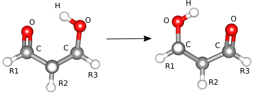
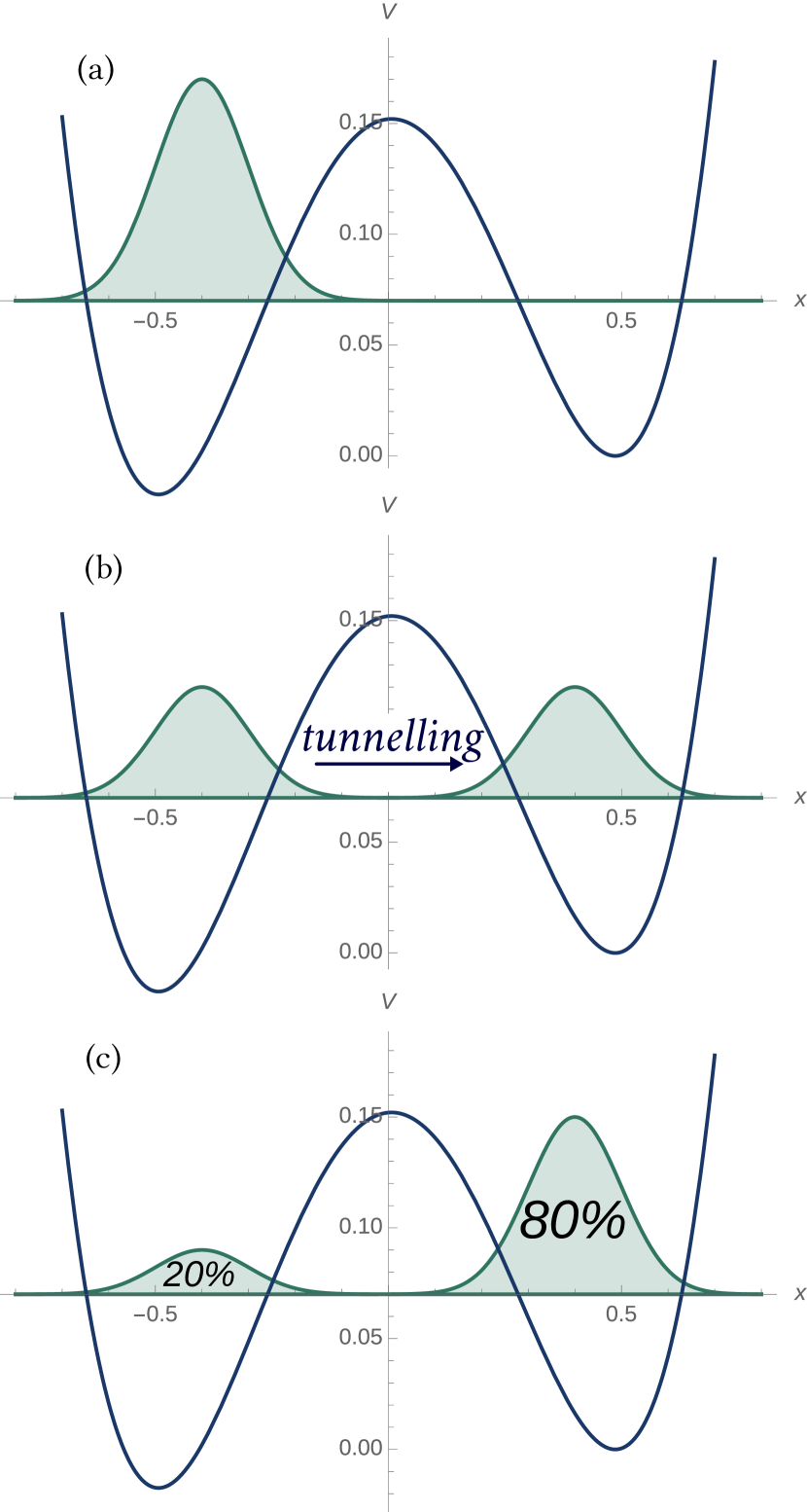
Scheme: There are different strategies that have been proposed in the literature to achieve laser-driven isomerization reaction. Here we have considered the method called "hydrogen-subway" proposed by N. Doslic et al. Doslic1998 where the wave packet representing the reactant state in the presence of applied laser field tunnels through the potential barrier and gives the product. The reaction process is shown in Fig. 1.
For the simulation of laser-driven isomerization reaction in one dimension, we consider the time-dependent Schrdinger’s equation
| (1) |
where the molecular Hamiltonian is given by
| (2) |
Here T is the kinetic energy operator and the asymmetric double-well quatric potential can be implemented by the potential energy operator as a function of position
| (3) |
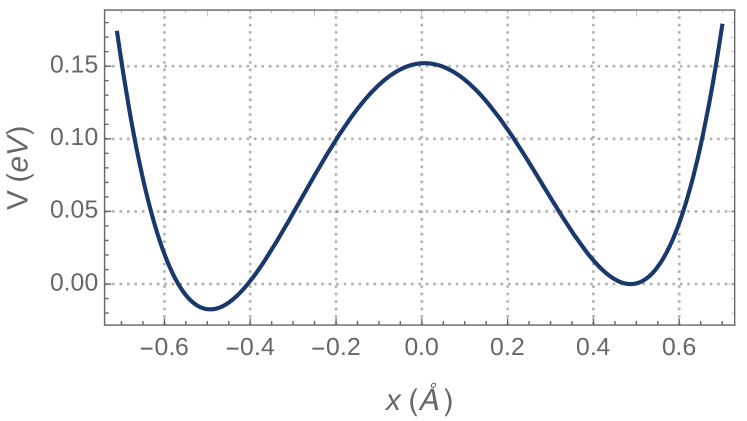
where gives the positions of the minima, represents the height of the barrier and the asymmetry of the wells can be changed by varying .
The laser-molecule interaction Hamiltonian is
| (4) |
where represents the dipole moment operator and is the driving electric field.
The time evolution of the system is given by
| (5) |
where the time evolution operator is given by the time-ordered integral
| (6) |
here is the time ordering operator. By using second order Trotter-Suzuki formula we can decompose the propagator as Wiebe2011 ; Poulin2015 ; qgs_sup_NielsenCUP2000 ; Daskin2011
| (7) |
Since the kinetic energy operator is diagonal in momentum basis, to make the simulation simpler, we perform quantum Fourier transform () . So the modified unitary evolution operator takes the following form
| (8) |
where the operators
In our experiments, we have considered a three qubit system to simulate the reaction dynamics. For that we discretize the space on lattice points with spacing , and we encode the wave function on quantum registers as
| (9) | ||||
Similarly, we divide the total time into 20 small time steps with interval . We show the reaction mechanism in three subsequent stages: (a) the initial time interval where the laser pulse is switched on, (b) the intermediate interval where the field is kept constant (c) the final stage where the field is turned off gradually. The behaviour of the electric field is given by Lu2011
For , the electric field at different time steps takes the values
Since we discretized the space using 8 grid points, the diagonal operators are given by
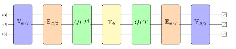
In Fig. 3, we have shown the circuit implementation for one time step evolution of the chemical reaction. We make use of Walsh-series approximation Welch2014 for implementing diagonal unitary operators without ancillas. The detailed method is explained in the supplemental material.
Initially we prepare our state in , which corresponds to the ground state of the reactant. During the time evolution we apply the electric field in such a way that the final state should approach the product state . After each time step we make the measurement to keep track of the reaction process.
Results: In Fig. 6 we have illustrated the reaction process in three different time intervals. Initially the reactant is localized in left potential well, by introducing the laser pulse the reactant starts converting into superposition of near-degenerate delocalized state. In the intermediate stage constant electric filed is applied, the wave packet representing the reactant starts to tunnels through the barrier. At the final stage we turn off the laser pulse, which results in the stabilization of wave function as product state in the right potential well.
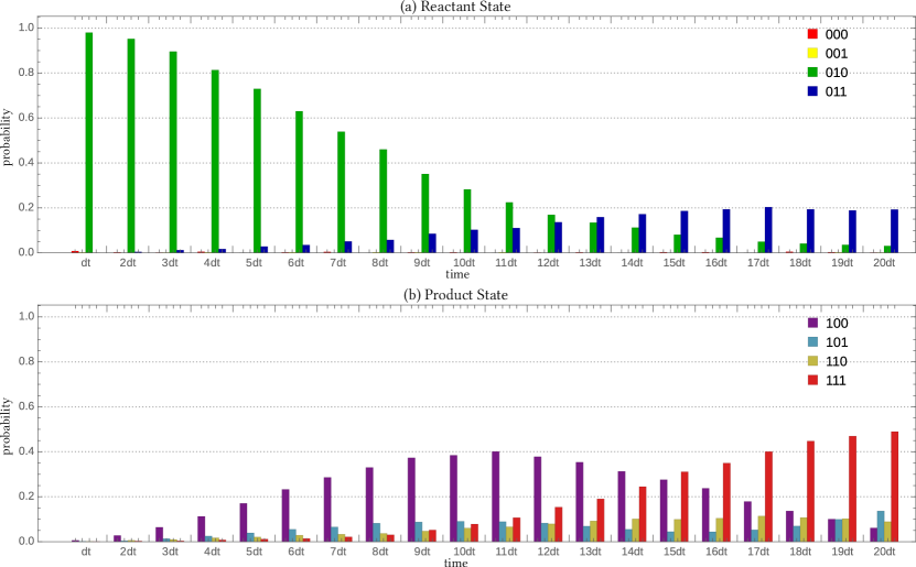
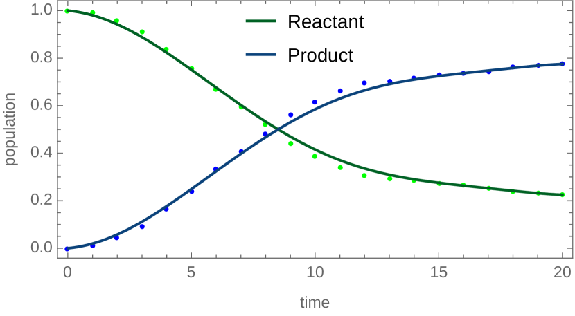
The probabilities of reactant and product state during twenty time step evolution is shown in Fig. 4. The continuous transformation of reactant to product state is clearly observed from the Fig. 5. At the end of the reaction the population of the product state reaches 78%.
The simulation has been performed in IBM’s ideal quantum simulator (ibmq_qasm_simulator) using 3 qubits. Since the number of gate operations are very large, using the quantum processor was impractical because of accumulation of gate errors.
Conclusion: To summarize, we have demonstrated quantum simulation of laser-driven chemical isomerization reaction in its entirety in 20 discrete time steps. In each time step we have discretized the wave function in position basis to keep track of the product yield and the progress of the reaction. The formation of product from reactant can be better understood as a tunneling phenomena through a potential barrier. The final state and the yield of product is in strong agreement with theoretical predictions.
Efficient simulation of polyatomic reactions is one of the biggest objective of quantum chemistry and quantum simulation. The method we have used to implement arbitrary diagonal operators in a quantum circuit do not require any ancillary qubits. Further, depending on the degree of discretization, the circuit can be easily scaled to any number of qubits.
Accurate simulation of reaction dynamics over a long stretch of time requires quantum processors that have high coherence time and low gate and readout error. All of the currently available open quantum computing platforms (IBM, Riggeti, etc.) have high gate errors that prohibit precise simulation of multi-molecular reactions for a long period of time. With proper error-correction, this simulation can be run on a quantum processor in future.
Author contributions: Theoretical analysis, design of quantum circuit and simulation were performed by N.N.H. and K.H. Collection and analysis of data was done by N.N.H. and K.H. The project was supervised by B.K.B. P.K.P. has thoroughly reviewed the manuscript. K.H., N.N.H. and B.K.B. have completed the project under the guidance of P.K.P.
Acknowledgements: We thank Indian Institute of Science Education and Research Kolkata for providing hospitality during which this work was completed. We acknowledge the support of IBM Quantum Experience for providing access to the quantum processors. The discussions and opinions developed in this paper are only those of the authors and do not reflect the opinions of IBM or any of it’s employees.
References
- (1) R. P. Feynman, Int. J. Theor. Phys. 21, 467 (1982).
- (2) I. Buluta and F. Nori, Science 326, 108 (2009).
- (3) S. Lloyd, Science 273, 1073 (1996).
- (4) A. Aspuru-Guzik, A. D. Dutoi, P. J. Love, and M. Head-Gordon, Science (80). 309, 1704 (2005).
- (5) R. Babbush, P. J. Love, and A. Aspuru-Guzik, Sci. Rep. 4, 6603 (2015).
- (6) B. P. Lanyon, J. D. Whitfield, G. G. Gillett, M. E. Goggin, M. P. Almeida, I. Kassal, J. D. Biamonte, M. Mohseni, B. J. Powell, M. Barbieri, A. Aspuru-Guzik, and A. G. White, Nat. Chem. 2, 106 (2010).
- (7) I. Kassal, S. P. Jordan, P. J. Love, M. Mohseni, and A. Aspuru-Guzik, Proc. Natl. Acad. Sci. 105, 18681 (2008).
- (8) I. Kassal, J. D. Whitfield, A. Perdomo-Ortiz, M.-H. Yung, and A. Aspuru-Guzik, Annu. Rev. Phys. Chem. 62, 185 (2011).
- (9) A. Kandala, A. Mezzacapo, K. Temme, M. Takita, M. Brink, J. M. Chow, and J. M. Gambetta, Nature 549, 242 (2017).
- (10) P. J. J. O’Malley, R. Babbush, I. D. Kivlichan, J. Romero, J. R. McClean, R. Barends, J. Kelly, P. Roushan, A. Tranter, N. Ding, B. Campbell, Y. Chen, Z. Chen, B. Chiaro, A. Dunsworth, A. G. Fowler, E. Jeffrey, E. Lucero, A. Megrant, J. Y. Mutus, M. Neeley, C. Neill, C. Quintana, D. Sank, A. Vainsencher, J. Wenner, T. C. White, P. V. Coveney, P. J. Love, H. Neven, A. Aspuru-Guzik, and J. M. Martinis, Phys. Rev. X 6, 031007 (2016).
- (11) I. D. Kivlichan, J. McClean, N. Wiebe, C. Gidney, A. Aspuru-Guzik, G. K.-L. Chan, and R. Babbush, Phys. Rev. Lett. 120, 110501 (2018)Phys. Rev. Lett. 120, 110501 (2018).
- (12) S. Sim, J. Romero, P. D. Johnson, and A. Aspuru-Guzik, Physics (College. Park. Md). 11, 14 (2018).
- (13) J. I. Colless, V. V. Ramasesh, D. Dahlen, M. S. Blok, M. E. Kimchi-Schwartz, J. R. McClean, J. Carter, W. A. de Jong, and I. Siddiqi, Phys. Rev. X 8, 011021 (2018).
- (14) A. T. Sornborger, P. Stancil, and M. R. Geller, Quantum Inf. Process. 17, 106 (2018).
- (15) A. Peruzzo, J. McClean, P. Shadbolt, M.-H. Yung, X.-Q. Zhou, P. J. Love, A. Aspuru-Guzik, and J. L. O’Brien, Nat. Commun. 5, 4213 (2014).
- (16) J. Du, N. Xu, X. Peng, P. Wang, S. Wu, and D. Lu, Phys. Rev. Lett. 104, 030502 (2010).
- (17) D. Lu, N. Xu, R. Xu, H. Chen, J. Gong, X. Peng, and J. Du, Phys. Rev. Lett. 107, 020501 (2011).
- (18) C. Hempel, C. Maier, J. Romero, J. McClean, T. Monz, H. Shen, P. Jurcevic, B. P. Lanyon, P. Love, R. Babbush, A. Aspuru-Guzik, R. Blatt, and C. F. Roos, Phys. Rev. X 8, 031022 (2018).
- (19) QiskitTM | Quantum Information Science Kit https://qiskit.org/.
- (20) N. N. Hegade, B. K. Behera, and P. K. Panigrahi, arXiv:1712.07326.
- (21) N. Doslic, O. Kuhn, J. Manz, and K. Sundermann, J. Phys. Chem. A 102, 9645 (1998).
- (22) N. Wiebe, D. W. Berry, P. Hoyer, and B. C. Sanders, J. Phys. A Math. Theor. 44, 445308 (2011).
- (23) D. Poulin, M. B. Hastings, D. Wecker, N. Wiebe, A. C. Doberty, and M. Troyer, Quantum Info. Comput. 15, 361-384 (2015).
- (24) M. A. Nielsen and I. L. Chuang, Quantum Computation and Quantum Information (Cambridge University Press, Cambridge, U.K., 2000)
- (25) A. Daskin and S. Kais, J. Chem. Phys. 134, 144112 (2011).
- (26) J. Welch, D. Greenbaum, S. Mostame, and A. Aspuru-Guzik, New J. Phys. 16, 033040 (2014).
- (27) Y. A. Geadah and M. J. G. Corinthios, IEEE Trans. Comput. C-26, 435 (1977).
- (28) I. M. Georgescu, S. Ashhab, and F. Nori, Rev. Mod. Phys. 86, 153 (2014).
- (29) Y. Mohanta, D. S. Abhishikth, K. Pruthvi, V. Kumar, B. K. Behera, and P. K. Panigrahi, arXiv:1807.00323.
- (30) Manabputra, B. K. Behera, and P. K. Panigrahi, arXiv:1806.10229.
SUPPLEMENTAL MATERIAL: Digital Quantum Simulation of Laser-Pulse Induced Tunneling Mechanism in Chemical Isomerisation Reaction
To implement an arbitrary diagonal unitary operator using quantum circuit we need to decompose it into a sequence of at most two-level unitary gates. This is an ardous task for most operators that we encounter in nature Daskin2011 . In this paper, we apply a method given by Welch et al. Welch2014 using Walsh function and Walsh operators without requiring any ancillary qubits. We demonstrate this method in qubits for one of the operators .
The discrete Walsh-Hadamard function (or Walsh function) is sampled by discretizing the interval into points, giving us where . Each element of the Walsh function can be obtained from
| (10) |
which for , gives us a matrix
| (11) |
For demonstration, we implement the operator as follows
| (12) |
The discretized eigenfunction for this operator is
| (13) |
The discrete Walsh-Fourier transform of is
| (14) |
The Walsh operator corresponding to it is found from the reversed binary string of . For instance, to find on qubits, we bit-reverse (which is ) and replace the zeros by identity and ones by Pauli Z gates. This gives us .
Using these pairs of Walsh-Fourier functions and Walsh operators, any n qubit diagonal operator can be expressed as a sequence of exponential unitary operators given by
| (15) |
Here the circuit for each operator is a rotation gate about axis given by where . To reduce number of redundant gates and gate error, we rearrange these operators in sequency order Geadah1997 . Using Eq. (14) we calculate the Walsh-Fourier coefficients and the corresponding rotations
| -19.041 | 38.083 | |||
| 0.377 | -0.754 | |||
| -18.127 | 36.254 | |||
| 0.363 | -0.727 | |||
| -18.796 | 37.593 | |||
| 0.349 | -0.698 | |||
| -18.362 | 36.725 | |||
| 0.357 | -0.713 | |||
Fig. 7 shows the optimal quantum circuit that uses Walsh operators to implement any diagonal unitary operator for three qubits.
