Eigenvalue Determination for Mixed Quantum States
using Overlap Statistics

Abstract

We consider the statistics of overlaps between a mixed state and its image under random unitary transformations. Choosing the transformations from the unitary group with its invariant (Haar) measure, the distribution of overlaps depends only on the eigenvalues of the mixed state. This allows one to estimate these eigenvalues from the overlap statistics. In the first part of this work, we present explicit results for qutrits, including a discussion of the expected uncertainties in the eigenvalue estimation. In the second part, we assume that the set of available unitary transformations is restricted to $SO(3)$, realized as Wigner $D$-matrices. In that case, the overlap statistics does not depend only on the eigenvalues, but also on the eigenstates of the mixed state under scrutiny. The overlap distribution then shows a complicated pattern, which may be considered as a fingerprint of the mixed state. When using random transformations from the unitary group, the eigenvalues can be determined quite simply from the lower and the upper limit of the overlap statistics. This may still be possible in the $SO(3)$ case, but only at the expense of a finite systematic uncertainty.

PhySH: quantum parameter estimation, quantum tomography, group theory, quantum measurements.

I Introduction

Quantum state tomography Paris and Rehacek (2004) deals with the complete characterization of an ensemble of identically and independently distributed quantum states. It involves the estimation of all elements of the density matrix describing that ensemble of states. As a consequence, experimental protocols become expensive and time consuming, even for medium sized quantum systems Häffner et al. (2005); Cramer et al. (2010). A natural reduction of the tomography problem consists of only estimating the eigenvalues of the density matrix. For such an approach, different experimental schemes have been proposed Keyl and Werner (2001); Ballester (2006); Tanaka et al. (2014); van Enk and Beenakker (2012).

The method to be discussed here is based on measuring the overlap between two mixed quantum states Walborn et al. (2006, 2007). This requires two copies of the quantum state, the possibility to apply unitary transformations to one of these copies, and finally a measurement of the overlap between the two states. Different schemes for overlap measurements are discussed for instance in Refs. Filip (2002); Bartkiewicz et al. (2013), while the experimental application of unitary transformations (together with complete tomography) has been shown, e.g., in “transmon” qutrits Bianchetti et al. (2010); a variant of the superconducting charge qubit. In Ref. Vitanov (2012), several scenarios have been proposed, which allow to realize general $SU(3)$ transformations in atomic three-level systems.

Our method is based on the fact that the distribution of overlaps $P_{\varrho}(q)$ between a given density matrix $\varrho$ and its image under random unitary transformations depends only on the eigenvalues of $\varrho$. These eigenvalues may then be estimated from the knowledge of $P_{\varrho}(q)$. For that, it is crucial to compute $P_{\varrho}(q)$ analytically, as this allows us to find convenient strategies to solve the inverse problem of estimating the eigenvalues. In order to compute $P_{\varrho}(q)$, we generalize previous results on the joint probability distribution of projection probabilities for random orthonormal quantum states Alonso and Gorin (2016). We then concentrate on the qutrit case, where we obtain $P_{\varrho}(q)$ in closed form.

There may be experimental situations, where the sampling over all unitary transformations is not possible, i.e., $SU(3)$ in the qutrit case. Therefore, we also consider the distribution of overlaps, when the transformations are restricted to rotations in real space. This amounts to consider a sub-group of $SU(3)$ that can be parametrized by the respective Wigner $D$-matrices Sakurai (1994). In this case, the overlap distribution actually contains more information about the original density matrix $\varrho$, not only the eigenvalues. However, in the absence of an analytical expression, the extraction of that information is much more difficult. Nevertheless, even in that case, our approach can provide important bounds for the eigenvalues of $\varrho$.

The paper is organized as follows: After this introduction, in Sec. II, we provide the mathematical and technical background for the overlap function. In Sec. III, we present the analytical calculation of the overlap distribution for the $SU(3)$ case. In Sec. IV, we compute the expected uncertainties of the eigenvalue estimation based on the upper and lower limit of the overlap distribution, themselves having been estimated with finite precision. In Sec. V, we discuss overlap distributions for transformations limited to $SO(3)$. Conclusions are provided in Sec.  VI.

II General definitions and notation

Let $\mathcal{H}$ be the Hilbert space of finite dimension $N={\rm dim}(\mathcal{H})$ corresponding to some quantum system. Let $\varrho$ be a mixed state with $N$ non-negative eigenvalues $\bm{\lambda}=(\lambda_{1},\lambda_{2},\ldots,\lambda_{N})$, normalized as $\sum_{j=1}^{N}\lambda_{j}=1$. We are then interested in the distribution of the values of the overlap function

$$Q(O,\varrho)={\rm tr}\big{(}\,O\,\varrho\,O^{\dagger}\,\varrho\,\big{)},$$ (1)

averaged over the whole unitary group with the respective Haar measure Haar (1933); Weyl (1939). In a different context, the same quantity has been considered as a measure for the distance between the reduced dynamics of two open quantum systems Znidaric and Prosen (2003); Gorin et al. (2006). Note that $Q(O,\varrho)$ does not depend on the value of the determinant of $O$, which means that the distribution over the unitary group or the corresponding special unitary group yields exactly the same result. Note also that for $O=\mathbb{1}$ the overlap function reduces to the purity, used in the area of quantum information Nielsen and Chuang (2000).

Our main interest is in the probability density

$$P_{\varrho}(q)=\langle\delta[q-Q(O,\varrho)]\rangle=\langle\delta[q-Q(O,\bm{\lambda})]\rangle\;,$$ (2)

where the angular brackets represent the average over the unitary group with respect to the normalized Haar measure. The second equality is valid due to the invariance of this measure. It means that $P_{\varrho}(q)$ depends only on the eigenvalues of $\varrho$  . In what follows, we will assume that the eigenvalues are arranged in ascending order: $\lambda_{\rm min}=\lambda_{1}\leq\lambda_{2}\leq\ldots\leq\lambda_{N}=\lambda_{\rm max}$. This can always be achieved, since permutations belong to the unitary group. Now, we may write,

$$Q(O,\bm{\lambda})=\sum_{j,k=1}^{N}\lambda_{j}\lambda_{k}|O_{jk}|^{2}=\sum_{k=1}^{N}t_{k}\lambda_{k}\;,$$

$$\text{where}\quad t_{k}=\sum_{j=1}^{N}\lambda_{j}|O_{jk}|^{2}\;.$$ (3)

The normalization of the column vectors of $O$ implies that $|O_{jN}|^{2}=1-\sum_{k=1}^{N-1}|O_{jk}|^{2}$. Using this, and the fact that density matrices have unit trace $\sum_{j=1}^{N}\lambda_{j}=1$, we may reduce the number of partial overlaps by one and write

$$Q(O,\bm{\lambda}) =\lambda_{N}+\sum_{k=1}^{N-1}t_{k}\,(\lambda_{k}-\lambda_{N})\;.$$ (4)

Therefore, we can calculate the overlap distribution $P_{\varrho}(q)$ from the joint probability distribution (JPD) as

$$\mathcal{P}_{\bm{\lambda}}(\bm{t}^{\prime})=\left\langle{\textstyle\prod_{k=1}^{N-1}\delta\left[t_{k}-\textstyle\sum_{j=1}^{N}\lambda_{j}|O_{jk}|^{2}\right]}\right\rangle,$$ (5)

for the partial overlaps $\bm{t}^{\prime}=(t_{1},t_{2},\ldots,t_{N-1})$, by the following $N-1$ dimensional integral:

$$P_{\varrho}(q)=\left\{\prod_{k=1}^{N-1}\int_{0}^{1}{\rm d}t_{k}\right\}\mathcal{P}_{\bm{\lambda}}(\bm{t}^{\prime})\;\delta\big{[}q-Q(O,\bm{\lambda})\,\big{]}.$$ (6)

The JPD $\mathcal{P}_{\bm{\lambda}}(\bm{t}^{\prime})$ can be calculated by generalizing an earlier work on the projection probabilities of random orthonormal states Alonso and Gorin (2016).

In the following Sec II.1, we discuss some special cases, where the calculation of the overlap distribution is particularly simple. This may help to prepare the ground for working out the general case, considered in Secs. III and IV.

II.1 Special cases for $N=2$ and $N=3$

In the qubit case, $N=2$, the overlap distribution can be obtained in general. In the qutrit case, $N=3$, we will consider special cases, where one or two eigenvalues of the density matrix are equal to zero.

In the qubit case, we find from Eqs. (3) and (4) that

$$Q(O, \varrho)=\lambda_{2}+(\lambda_{1}-\lambda_{2})\;t_{1}\;,$$ (7)

$$t_{1}=\lambda_{1}|O_{11}|^{2}+\lambda_{2}|O_{21}|^{2}=\lambda_{2}+(\lambda_{1}-\lambda_{2})\;|O_{11}|^{2}\;,$$

such that the overlap function is given by

$$Q(O,\varrho)=2\lambda_{1}\lambda_{2}+(\lambda_{1}-\lambda_{2})^{2}\;|O_{11}|^{2}\;.$$ (8)

The overlap depends linearly on the absolute value squared of the random unitary matrix $O\in U(2)$. In Ref. Alonso and Gorin (2016), the distribution of sums of $K$ such absolute values squared have been calculated as averages over $U(N)$, denoted by $\mathcal{P}_{NK}(t)$. For the present case, we may set $t=|O_{11}|^{2}$ and find $\mathcal{P}_{21}(t)=\Theta(t)\,\Theta(1-t)$, where $\Theta(t)$ is the unit step function.

With the maximum (minimum) value for $Q(O,\varrho)$ is given by

$$q_{\rm max}=\lambda_{1}^{2}+\lambda_{2}^{2}\quad\text{and}\quad q_{\rm min}=2\lambda_{1}\lambda_{2}\;,$$ (9)

respectively, we obtain

$$P_{\varrho}(q) =\langle\,\delta\left[q-Q(O,\varrho)\right]\,\rangle$$

$$=\int_{0}^{1}{\rm{d}}t\;\mathcal{P}_{21}(t)\;\delta\big{[}\,q-(2\lambda_{1}\lambda_{2}+(\lambda_{1}-\lambda_{2})^{2}\;t)\,\big{]}$$

$$=\frac{\Theta(q-q_{\rm min})\,\Theta(q_{\rm max}-q)}{(\lambda_{1}-\lambda_{2})^{2}}\;.$$ (10)

In Fig. 1 (a), we show the distribution $P_{\varrho}(q)$ for several values of $\lambda_{1}$ and $\lambda_{2}$. A delta distribution is reached when $\lambda_{1}=\lambda_{2}$. Due to the unit trace property, $\lambda_{1}+\lambda_{2}=1$, any single quantitative property of the overlap distribution is enough to estimate the eigenvalues of $\varrho$. This quantity might be its maximum value, $(\lambda_{1}-\lambda_{2})^{-2}$, $q_{\rm max}$ or $q_{\rm min}$. Experimentally, the easiest case would consist in measuring $q_{\rm max}$ which turns out to be the purity of our the mixed state, showing that a random sampling can be spared entirely in this case.

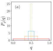
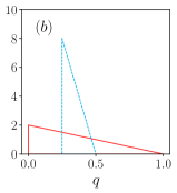
Figure 1: (Color online) Overlap probability density $P_{\varrho}(q)$ for $N=2\,(3)$ and different sets of eigenvalues. Panel (a) shows the qubit case: $\lambda_{1}\,(\lambda_{2})=0\,(1)$ (red solid line), $\lambda_{1}\,(\lambda_{2})=0.2\,(0.8)$ (orange dot dashed line), $\lambda_{1}\,(\lambda_{2})=0.3\,(0.7)$ (blue dashed line), and $\lambda_{1}\,(\lambda_{2})=0.4,(0.6)$ (green dotted line). Panel (b) shows the qutrit case: $\lambda_{1}=\lambda_{2}=0\,,\;\lambda_{3}=1$ (red solid line), and $\lambda_{1}=0\,,\;\lambda_{2}=\lambda_{3}=0.5$ (blue dashed line).

Even for the mixed state of a qutrit ($N=3$), it is possible to obtain simple expressions for the overlap distribution, in some special cases. The line of argument is analogous to the qubit case, and we delegate the corresponding discussion to App. A. In Fig. 1(b), we show two of these cases, $\lambda_{1}=0\,,\;\lambda_{2}=\lambda_{3}=1/2$, where

$$P_{\varrho}(q)=16\,(1-2q)\;\Theta(q-1/4)\;\Theta(1/2-q)\;,$$ (11)

and $\lambda_{1}=\lambda_{2}=0\,,\;\lambda_{3}=1$, where

$$P_{\varrho}(q)=2\,(1-q)\;\Theta(q)\;\Theta(1-q)\;.$$ (12)

In order to estimate the eigenvalues of an arbitrary mixed qutrit state, we would need two quantitative properties of the overlap distribution. In this work we will concentrate on the limits $q_{\rm max}$ and $q_{\rm min}$ of $P_{\varrho}(q)$.

III JPD for general case

In this section, we derive a general integral expression for the joint probability density defined in Eq. (5). We will closely follow the derivation for the unitary case in Ref. Alonso and Gorin (2016). According to this work, Eq. (5) can be written as

$$\mathcal{P}_{\bm{\lambda}}(\bm{t}^{\prime})\propto\left\{{\textstyle\prod_{k=1}^{N-1}}\int d\Omega_{2}(\bm{w}_{k})\;\right.$$

$$\times\left.\delta\Big{(}t_{k}-{\textstyle\sum_{j=1}^{N}}\lambda_{j}|w_{jk}|^{2}\Big{)}\right\}\;\prod_{\mu<\nu}^{N-1}\delta^{2}\big{(}\langle\bm{w}_{\mu}\,|\,\bm{w}_{\nu}\rangle\big{)}\;.$$ (13)

Here, $d\Omega_{2}(\bm{w}_{\xi})$ denotes the uniform measure on the hypersphere in $\mathbb{R}^{2N}$, which implements the normalization of the column vectors $\bm{w}_{\xi}$ of $O$. Correspondingly, the last product of delta functions implements the orthogonality conditions between these column vectors. In that case, the delta-function is two-dimensional because for $\langle\bm{w}_{\mu}|\bm{w}_{\nu}\rangle$ to be zero, the real and the imaginary part must be zero. The integral expression on the RHS is proportional to $\mathcal{P}_{\bm{\lambda}}(\bm{t}^{\prime})$ such that one has to compute the normalization constant for $\mathcal{P}_{\bm{\lambda}}(\bm{t}^{\prime})$, separately.

Following the steps described in Ref. Alonso and Gorin (2016), we arrive at the following result:

$$\mathcal{P}_{\bm{\lambda}}({\bf{t}}^{\prime}) =\frac{1}{Z(\bm{o})}\left\{\prod_{k=1}^{N-1}\int\frac{ds_{k}}{2\pi}\right\}Z(\bm{s})\;,$$ (14)

where $Z(\bm{s})$ and the matrix $\bm{C}$, it depends upon, are defined as

$$Z(\bm{s}) =\left\{\prod_{\mu<\nu}^{N-1}\int\frac{d^{2}\tau_{\mu\nu}}{4\pi^{2}}\right\}\frac{1}{\prod_{j=1}^{N}\det[\bm{C}(\lambda_{j})]}\;,$$ (15)

$$\bm{C}(\lambda) =\left(\begin{array}[]{ccc}c_{1}(\lambda)&\tau/2&\ldots\\ -\tau^{*}/2&c_{2}(\lambda)&\\ \vdots&&\ddots\end{array}\right)\;,$$ (19)

with $c_{j}(\lambda)=1-is_{j}(\lambda-t_{j})$. The matrix $\bm{C}$ is a $N-1$ dimensional square matrix which contains the $\mathbf{t^{\prime}}$ parameters. In the following Sec. III.1, we compute $\mathcal{P}_{\bm{\lambda}}({\bf{t}}^{\prime})$ for the qutrit case $N=3$.

III.1 JPD for $N=3$

Let us assume the ordering $\lambda_{1}<\lambda_{2}<\lambda_{3}$, and write the overlap function as

$$Q(O,\varrho) =\lambda_{3}-t_{1}\;(\lambda_{3}-\lambda_{1})-t_{2}\;(\lambda_{3}-\lambda_{2})\;.$$ (20)

Then, we need to calculate

$$\mathcal{P}_{\bm{\lambda}}(t_{1},t_{2}) =\frac{1}{Z(\bm{o})}\left\{{\prod_{k=1}^{2}}\int\frac{\text{d}s_{k}}{2\pi}\right\}\;Z(\bm{s})\;,$$ (21)

$$Z(\bm{s}) =\int\frac{\text{d}^{2}\tau}{4\pi^{2}}\frac{1}{\prod_{j=1}^{3}\det[\bm{C}(\lambda_{j})]}\;,$$ (22)

where the matrix $\bm{C}(\lambda)$ is defined as

$$\bm{C}(\lambda)=\left(\begin{array}[]{cc}c_{1}(\lambda)&\tau/2\\ -\tau^{*}/2&c_{2}(\lambda)\end{array}\right)\;,$$ (23)

with $c_{j}(\lambda)=1-is_{j}(\lambda-t_{j})$. As in Ref. Alonso and Gorin (2016), let us start with the integral

$$\int\frac{\text{d}s_{1}}{2\pi}\;\frac{1}{\prod_{j=1}^{3}\det[\bm{C}(\lambda_{j})]},$$ (24)

which can be calculated quite simply with the help of the residue theorem. To this end, we note that each determinant gives rise to one single pole at the position

$$\det\,\bm{C}(\lambda)=0\ \Leftrightarrow\ 1-is_{1}(\lambda-t_{1})=\frac{-|\tau|^{2}}{4\,c_{2}(\lambda)}$$

$$\Leftrightarrow\ s_{1}=\frac{i}{t_{1}-\lambda}\left[\,1+\frac{|\tau|^{2}}{4\,c_{2}(\lambda)}\,\right]\;.$$ (25)

Even though $c_{2}(\lambda)$ is complex, this does not affect the sign of the imaginary part of the pole. The pole lies on the upper (lower) half plane for $\lambda<t_{1}$ ($\lambda>t_{1}$). Since we may close the integration path either over the upper or the lower half plane, the integral is non-zero only if the two poles are lying on opposite sides of the real axis. This implies that there are only two cases of a non-zero result:

$$\text{a)}\quad 0<\lambda_{1}<t_{1}<\lambda_{2}<\lambda_{3}\;,$$

$$\text{b)}\quad 0<\lambda_{1}<\lambda_{2}<t_{1}<\lambda_{3}\;.$$

In both cases, the evaluation of all integrals is a rather tedious exercise, the description of which can be found in App. B.1 and App. B.2, with the respective results given in the Eqs. (77) and (86). These can be combined into one single expression:

$$\mathcal{P}_{\bm{\lambda}}(t_{1},t_{2}) =\frac{1}{h}\begin{cases}F(\lambda_{1},\lambda_{3},\lambda_{2})-F(\lambda_{1},\lambda_{2},\lambda_{3})&:\text{a)}\\ F(\lambda_{1},\lambda_{3},\lambda_{2})-F(\lambda_{3},\lambda_{2},\lambda_{1})&:\text{b)}\end{cases}\;,$$ (26)

where

$$F(a,b,c) =|t_{1}-a+t_{2}-b|+|t_{2}-c|\;,$$

$$\text{and}\quad h =(\lambda_{1}-\lambda_{2})(\lambda_{1}-\lambda_{3})(\lambda_{2}-\lambda_{3})\;.$$ (27)

Equation (26) provides the central result of this work. While it is probably difficult to determine this JPD directly, it allows to calculate the overlap distribution $P_{\varrho}(q)$ in closed form; see Sec. III.2, below.

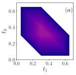
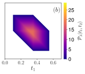
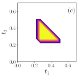
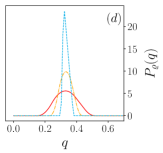
Figure 2: (Color online) Joint probability density $\mathcal{P}_{\bm{\lambda}}(t_{1},t_{2})$ for different sets of eigenvalues: (a) $\lambda_{1}=0.05,\;\lambda_{2}=0.3$, (b) $\lambda_{1}=0.1,\;\lambda_{2}=0.35$, and (c) $\lambda_{1}=0.22,\;\lambda_{2}=0.27$. Panel (d) shows the corresponding overlap distribution $P_{\varrho}(q)$. Red solid line (a), orange dot-dashed line (b), and blue dashed line (c).

In Fig. 2, panels (a), (b) and (c), we show $\mathcal{P}_{\bm{\lambda}}(t_{1},t_{2})$ for different sets of eigenvalues. The color coding is such that low (high) probability densities are represented by dark (bright) colors, while areas where the probability density is equal to zero are left white. This allows to identify that region in the $(t_{1},t_{2})$ plane, where the probability density, $\mathcal{P}_{\bm{\lambda}}(t_{1},t_{2})$, is larger than zero. The region of non-zero probability density may be characterized as the intersection of two simple geometric sets, the rectangular region $\lambda_{1}<t_{1},t_{2}<\lambda_{3}$ and the infinite stripe $\lambda_{1}+\lambda_{2}<t_{1}+t_{2}<\lambda_{2}+\lambda_{3}$. The surface defined by $\mathcal{P}_{\bm{\lambda}}(t_{1},t_{2})$ consists of seven planar triangles, stitched together to form a continuous polyhedron with an open hexagonal base and a horizontal top central triangle. When two eigenvalues become equal, but different from the third, the polyhedron reduces to a right triangular prism, and when all three eigenvalues become equal, the JPD becomes a two-dimensional delta distribution, centered at $t_{1}=t_{2}=1/3$. The overlap distribution $P_{\varrho}(q)$, shown in panel (d), will be discussed separately in Sec. III.2.

III.2 Overlap distribution function for a qutrit

The JPD for partial overlaps $t_{1}$ and $t_{2}$, discussed in the previous section is not directly measurable, but it allows to calculate the overlap probability density.

$$P_{\varrho}(q) =\langle\delta(q-Q(O,\varrho))\rangle$$

$$=\int_{0}^{1}{\rm{d}}t_{1}\int_{0}^{1}{\rm{d}}t_{2}\;\mathcal{P}_{\lambda}(t_{1},t_{2})\;\delta(q-Q(O,\varrho))\;.$$ (28)

The variable transformation,

$$t_{2}\to q^{\prime}=\lambda_{3}-(\lambda_{3}-\lambda_{1})\;t_{1}-(\lambda_{3}-\lambda_{2})\;t_{2}\;,$$

allows us to evaluate the $t_{2}$-integral eliminating the delta-function:

$$P_{\varrho}(q) =\frac{1}{\lambda_{3}-\lambda_{2}}\int_{0}^{1}{\rm{d}}t_{1}\int_{\lambda_{2}-(\lambda_{3}-\lambda_{1})t_{1}}^{\lambda_{3}-(\lambda_{3}-\lambda_{1})t_{1}}{\rm{d}}q^{\prime}$$

$$\times\mathcal{P}_{\bm{\lambda}}\left(t_{1},\frac{\lambda_{3}-q^{\prime}-(\lambda_{3}-\lambda_{1})t_{1}}{\lambda_{3}-\lambda_{2}}\right)\delta(q-q^{\prime})\;.$$ (29)

Since $q^{\prime}$ is limited to the interval

$$\big{(}\,\lambda_{2}-(\lambda_{3}-\lambda_{1})t_{1}\,,\,\lambda_{3}-(\lambda_{3}-\lambda_{1})t_{1}\,\big{)}\;,$$

the $q^{\prime}$ integral contributes to the overlap probability density, only if $q$ is lying in the same interval. That leads to the following additional restrictions for $t_{1}$:

$$t_{1}<\frac{\lambda_{3}-q}{\lambda_{3}-\lambda_{1}}\;,\quad\text{and}\quad t_{1}>\frac{\lambda_{2}-q}{\lambda_{3}-\lambda_{1}}\;.$$ (30)

Therefore, we obtain

$$P_{\varrho}(q)=\int_{t_{1}^{\min}}^{t_{1}^{\max}}{\rm d}t_{1}\;\mathcal{P}_{\bm{\lambda}}\left(t_{1},\frac{\lambda_{3}-q-(\lambda_{3}-\lambda_{1})t_{1}}{\lambda_{3}-\lambda_{2}}\right)\;,$$ (31)

where the new integration bounds are given by

$$t_{1}^{\min} =\max\left(0,\frac{\lambda_{2}-q}{\lambda_{3}-\lambda_{1}}\right)\;,\quad t_{1}^{\max}=\min\left(1,\frac{\lambda_{3}-q}{\lambda_{3}-\lambda_{1}}\right)\;.$$ (32)

Since $\mathcal{P}_{\bm{\lambda}}(t_{1},\alpha+\beta\,t_{1})$ is a piecewise linear function, the integration is straightforward for any particular case. As a result, $P_{\varrho}(q)$ becomes piecewise quadratic. In Fig. 2, panel (d), $P_{\varrho}(q)$ is plotted for the combination of eigenvalues considered in the first three panels of Fig. 2.

III.3 Range of the overlap distribution

The range of the overlap probability density, $P_{\varrho}(q)$ is limited to a finite interval: $q_{\rm min}<q<q_{\rm max}$, with limits depending on the eigenvalues of $\varrho$. Here, we will show that it is typically enough to know these limits, in order to estimate the eigenvalues of $\varrho$.

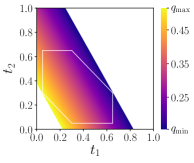
Figure 3: (Color online) The overlap $q(t_{1},t_{2})$ as a color coded density plot, as defined in Eq. (33), for $\lambda_{1}=0.05$ and $\lambda_{2}=0.3$. In this case, $q_{\rm min}=0.155$ and $q_{\rm max}=0.515$.

Based on Eq. (20), we may write the overlap $Q(O,\varrho)$ as a function of the partial overlaps, $t_{1},t_{2}$ defined in Eq. (3):

$$q(t_{1},t_{2})=\lambda_{3}-t_{1}\;(\lambda_{3}-\lambda_{1})-t_{2}\;(\lambda_{3}-\lambda_{2})\;.$$ (33)

In Fig. 3, we show a density plot of this function, where we chose for the eigenvalues the case (a) from Fig. 2. The white lines indicate the limits of the range of $\mathcal{P}_{\bm{\lambda}}(t_{1},t_{2})$. It can be seen that equipotential lines are straight lines, with the overlap value $q$ increasing towards the origin of the $(t_{1},t_{2})$-plane. On the basis of the discussion below Eq. (27), one readily verifies that the maximum value $q_{\rm max}$ is reached at the point $(t_{1},t_{2})=(\lambda_{1},\lambda_{2})$, whereas the minimum value is reached at $(t_{1},t_{2})=(\lambda_{3},\lambda_{2})$. Consequently, the maximum (minimum) value of $q$ is given by

$$q_{\rm max}=\lambda_{1}^{2}+\lambda_{2}^{2}+\lambda_{3}^{2}\quad\text{and}\quad q_{\rm min}=\lambda_{2}^{2}+2\lambda_{1}\lambda_{3}\;,$$ (34)

respectively. The upper limit $q_{\rm max}$ is of course just the purity of the mixed state $\varrho$, which can be obtained by choosing the identity for the unitary transformation in $Q(O,\varrho)$. To the best of our knowledge, the expression for the lower limit is a new result.

IV Stability of the eigenvalue estimation

Let us consider the task of estimating the eigenvalues of a mixed quantum state $\varrho$ from the statistics of overlaps. For that purpose, we assume that an experiment is realized, where overlaps are measured for a large but finite sample of random unitary transformations. The result of the experiment may be represented in the form of a histogram, which should approximate the true overlap distribution $P_{\varrho}(q)$. Since the sample is finite, the histogram will show deviations from the true distribution, and this will lead to uncertainties in the estimation of the eigenvalues.

A particularly simple procedure consists in using the experimental data to estimate $q_{\rm min}$ and $q_{\rm max}$, with uncertainties $\Delta q_{\rm min}$ and $\Delta q_{\rm max}$, respectively. In the case of qutrits, the knowledge of these two quantities is sufficient to determine the desired eigenvalues of the mixed quantum state under investigation. In what follows, we assume normally distributed errors, to compute the propagated uncertainties on these eigenvalues.

Resolving Eq. (34) for $\lambda_{1}$ and $\lambda_{2}$, taking into account that $\lambda_{1}+\lambda_{2}+\lambda_{3}=1$, we find

$$\lambda_{2} =\frac{1-\sqrt{3(q_{\rm max}+q_{\rm min})-2}}{3},$$ (35)

$$\lambda_{1} =\frac{1-\lambda_{2}-\sqrt{q_{\rm max}-q_{\rm min}}}{2}\;.$$ (36)

To work out the error propagation for $\lambda_{1}$ and $\lambda_{2}$, let us introduce the auxiliary parameters,

$$r=q_{\rm max}+q_{\rm min}\;,\qquad s=q_{\rm max}-q_{\rm min}\;,$$ (37)

which have both the same statistical error

$$\Delta^{2}=\Delta q_{\rm min}^{2}+\Delta q_{\rm max}^{2}\;.$$ (38)

Then, we obtain

$$(\Delta\lambda_{2})^{2}=\left(\frac{\partial\lambda_{2}}{\partial r}\right)^{2}\;\Delta^{2}=\frac{r^{2}}{4\,(3r-2)}\;\Delta^{2}\;.$$ (39)

Similarly,

$$(\Delta\lambda_{1})^{2} =\left(\frac{\partial\lambda_{1}}{\partial r}\right)^{2}\;\Delta^{2}+\left(\frac{\partial\lambda_{1}}{\partial s}\right)^{2}\;\Delta^{2}$$

$$=\left(\frac{r^{2}}{3r-2}+\frac{1}{s}\right)\frac{\Delta^{2}}{16}\;.$$ (40)

Finally,

$$\frac{(\Delta\lambda_{2})}{\Delta}=\frac{r}{2\,\sqrt{3r-2}}\;,\quad\frac{(\Delta\lambda_{1})}{\Delta}=\frac{1}{4}\,\sqrt{\frac{r^{2}}{3r-2}+\frac{1}{s}}\;.$$ (41)

These two expressions show that the uncertainty on the estimated eigenvalues can be kept small, as long as $r\neq 2/3$ and $s\neq 0$. According to Eq. (35), the first condition implies that $\lambda_{2}=1/3$, $\lambda_{1}+\lambda_{3}=2/3$; remember the ordering of the eigenvalues: $\lambda_{1}<\lambda_{2}<\lambda_{3}$. The second condition implies that $q_{\rm max}=q_{\rm min}$ which means that all eigenvalues must be equal. This situation is a limiting case of the first condition.

V Overlap function for Wigner $D$-matrices

In this section, we assume that the unitary transformations to be applied to the system are limited to $SO(3)$, the subgroup of rotations in $3D$ coordinate space. Examples of such systems are qutrits build from photon pairs Burlakov et al. (2003).

A natural parametrization for the subgroup $SO(3)$, is provided by the Wigner $D$-matrices for angular momentum quantum number $j=1$.

$$D=\left(\begin{array}[]{ccc}\frac{1+\cos\beta}{2}e^{-i(\alpha+\gamma)}&\frac{-e^{-i\alpha}}{\sqrt{2}}\sin\beta&\frac{1-\cos\beta}{2}e^{-i(\alpha-\gamma)}\\ \frac{e^{-i\gamma}}{\sqrt{2}}\sin\beta&\cos\beta&\frac{-e^{i\gamma}}{\sqrt{2}}\sin\beta\\ \frac{1-\cos\beta}{2}e^{i(\alpha-\gamma)}&\frac{e^{i\alpha}}{\sqrt{2}}\sin\beta&\frac{1+\cos\beta}{2}e^{i(\alpha+\gamma)}\end{array}\right).$$ (42)

Thus, we are interested in the distribution of

$$Q(D,\varrho)={\rm Tr}\big{[}\,D\,\varrho\,D^{\dagger}\;\varrho\,\big{]}\;.$$ (43)

Here, we can no longer assume that some transformation $D$ will diagonalize $\varrho$. As a consequence, the distribution of overlaps will depend not only on the eigenvalues of $\varrho$, but also on its eigenstates. To make this dependence clear, we assume that $\varrho$ is diagonalized by the unitary matrix $U$: $\varrho=U\,\underline{\lambda}\,U^{\dagger}$. Then, we may write

$$Q(D,\varrho) =Q(D,U,\underline{\lambda})=\text{Tr}\left[D\,U\,\underline{\lambda}\,U^{\dagger}\,D^{\dagger}\,U\underline{\lambda}\,U^{\dagger}\right]$$

$$=\text{Tr}\left[\tilde{D}\,\underline{\lambda}\,\tilde{D}^{\dagger}\,\underline{\lambda}\right],\quad\tilde{D}=U^{\dagger}\,D\,U\;.$$ (44)

Varying the angles $\alpha,\beta,\gamma$, moves $\tilde{D}$ along a three-dimensional orbit within the group $SU(3)$, where the orbit itself is determined by the eigenvector matrix $U$.

Our aim is the estimation of the eigenvalues of $\varrho$ from the overlap distribution $P_{\varrho}(q)$, under a random (or systematic) sampling over the Wigner $D$-matrices. This is now much more complicated, since $P_{\varrho}(q)$ now also depends on the eigenvectors of $\varrho$, collected as column vectors in $U$.

For instance, in the previous section we showed that it is sufficient to determine $q_{\rm min}$ and $q_{\rm max}$ in order to estimate the eigenvalues, since there we got two equations for two unknowns. However, here we have many additional unknowns for the eigenvectors. Therefore, on should expect that the determination of $q_{\rm min}$ and $q_{\rm max}$ will no longer be sufficient. In what follows, we use again the JPD of partial overlaps, $\mathcal{P}_{\varrho}(t_{1},t_{2})$ together with the full overlap distribution $P_{\varrho}(q)$, to analyze this problem.

V.1 Density matrices with randomly chosen eigenvectors

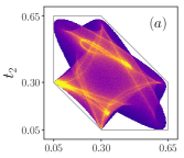
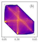
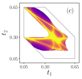
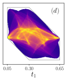
Figure 4: (Color online) Density of points $(t_{1},t_{2})$, Eq. (45), for different random unitary matrices; panels (a), (b), (c) and (d). The color coding reflects the density of points, such that regions with a higher (lower) density are plotted in yellow (purple). In the white regions no hits were found.

In this section, we consider density matrices with fixed eigenvalues $\lambda_{1}=0.05,\lambda_{2}=0.3$ (the same eigenvalues as in Figs. 2 and 3), but choose their eigenvector matrix $U$ at random from the full group $SU(3)$. We then compute a large sample (10 million elements) of pairs of partial overlaps, $(t_{1},t_{2})$ according to the expression

$$t_{k}=\lambda_{1}\;|\,\tilde{D}_{1k}\,|^{2}+\lambda_{2}\;|\,\tilde{D}_{2k}\,|^{2}+\lambda_{3}\;|\,\tilde{D}_{3k}\,|^{2}\;,$$ (45)

obtained from Eq. (44). Here, each pair $(t_{1},t_{2})$ is obtained from a Wigner $D$-matrix, with angles $\alpha,\beta,\gamma$ chosen from uniform distributions.

In Fig. 4 we plot an approximation to $\mathcal{P}_{\varrho}(t_{1},t_{2})$, in the form of a density plot for the sample of partial overlaps mentioned above. For each of the four panels, a different random matrix $U$ of eigenvectors has been chosen, and all of them for the same combination of eigenvalues $\lambda_{1}=0.05$ and $\lambda_{2}=0.3$. These plots are obtained by color coding the number of points $(t_{1},t_{2})$ hitting the area of each pixel on the graph (dark regions, mean a low density of points; bright regions a high density; regions without points were left white). The $SU(3)$ limits for the support of $\mathcal{P}_{\varrho}(t_{1},t_{2})$, obtained in Sec. III, are plotted by thin solid lines.

In all cases, it is possible to reach $q_{\rm max}$ at $(t_{1},t_{2})=(\lambda_{1},\lambda_{2})$. This is because the identity is an element of $SO(3)$ also. By contrast, it may not be possible to reach $q_{\rm min}$ at $(t_{1},t_{2})=(\lambda_{3},\lambda_{2})$. A very clear example for that is shown in panel (c). By contrast, panel (d) shows a case, where it seems that $q_{\rm min}$ is reached.

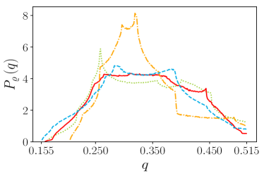
Figure 5: (Color online) Overlap distribution $P_{\varrho}(q)$ for the cases, corresponding to the four panels in Fig. 4. Green dotted line [panel (a)], red solid line [panel (b)], orange dot-dashed line [panel (c)], and blue dashed line [panel (d)].

Similarly, in Fig. 5, we plot an approximation to the total overlap distribution $P_{\varrho}(q)$, in the form of a histogram over the total overlaps $q$, computed according to Eq. (20). The histograms are calculated from the four data sets shown in Fig. 4. The different distributions posses a number of particularities, which may serve as a fingerprint for the density matrix under investigation. This means that using the overlap distribution, it is easy to distinguish different density matrices. However, so far we are not aware of any method to solve the inverse problem of determining eigenvalues and orientation of the eigenvectors, given the overlap distribution.

As mentioned before, in all cases, the overlap distribution reaches the maximal value $q_{\rm max}$, which is simply the purity of the density matrix in question. However, depending on the orientation of the eigenvectors, the minimum value $q_{\rm min}$ may or may not be reached; c.f. discussion of Fig. 4.

In Sec. III.3, we discussed the error propagation in the estimation of the eigenvalues of $\varrho$, based on measured values for $q_{\rm min}$ and $q_{\rm max}$. Based on this discussion, we find that it may be possible to obtain at least approximate estimates for the eigenvalues of $\varrho$, if the minimum value for $Q(D,\varrho)$ over the Wigner-$D$ matrices is sufficiently close to the absolute minimum, $q_{\rm min}$.

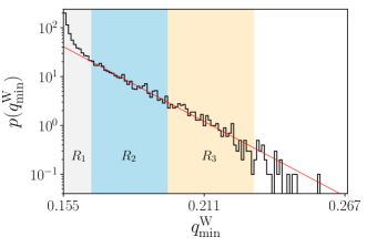
Figure 6: (Color online) Probability distribution for $q_{\rm min}$ over an ensemble of unitary matrices. The red line is fitted to the histogram’s tail, see main text for more details.

For that reason we study the distribution of minimum values,

$$q^{\rm W}_{\rm min}=\min_{D}Q(D,\varrho)\;,$$ (46)

in Fig. 6. For that purpose, we chose $10^{4}$ eigenvector matrices $U$ at random, searching for each one the minimum of $Q(D,\varrho)$ over $10^{5}$ randomly chosen Wigner matrices. Of course, this provides only a numerical approximation to the true distribution of minimum values $q^{\rm W}_{\rm min}$. The resulting distribution, again for $\lambda_{1}=0.05$ and $\lambda_{2}=0.3$, is shown in Fig. 6. We checked that a duplication of the sample of Wigner $D$-matrices would yield an indistinguishable result.

The minimum values $\min_{D}Q(D,\varrho)$ are restricted to the interval $[q_{\rm min},q_{\rm wc}]$, where the latter is calculated in the following Sec. V.2. Both quantities only depend on the eigenvalues of the mixed state $\varrho$ to be analyzed. The latter, $q_{\rm wc}$, is the largest possible minimum value $q^{\rm W}_{\rm min}$, which depends on the eigenvector matrix $U$. In Fig. 6, it can be seen that for the majority of eigenvector matrices, $q^{\rm W}_{\rm min}$ is rather close to $q_{\rm min}=0.155$ and rather far away from $q_{\rm wc}=0.267$, which means that with high probability, we may obtain useful estimates for the eigenvalues of $\varrho$, with reasonably small uncertainties. To illustrate this fact, we highlight the regions $R_{1}$, $R_{2}$ and $R_{3}$, with the following significance: In region $R_{1}$ we have $68.3\%$ of the counts, in $R_{1}+R_{2}$ it is $95.4\%$, and if we combine all the regions, $R_{1}+R_{2}+R_{3}$ the count is $99.7\%$. These percentage values are taken from the familiar $68$-$95$-$99.7$ rule of statistical significance tests.

V.2 Maximin overlap

In game theory, “maximin” is a term used to describe the strategy which maximizes one’s own minimum gain. Similarly, we consider here the maximum of the minimum overlap, where the minimum is taken over the Wigner $D$ matrices, and the maximum subsequently over all possible eigenvector matrices of $\varrho$. Thus

$$q_{\rm wc}=\max_{U\in SU(3)}\;\min_{D}\;Q(D,\varrho)=\max_{U\in SU(3)}\;q_{\rm min}^{\rm W}\;.$$ (47)

Depending on the eigenvectors of $\varrho$, $q_{\rm min}^{\rm W}$ may be considerably larger than the absolute minimum value $q_{\rm min}$, calculated in Sec. III.3, as has been shown in Fig. 6.

In the present section, we search for those eigenvector matrices $U$ that lead to the largest minimum value $q_{\rm wc}$. We conjecture that we may restrict our search to the set of permutation matrices:

$$U_{(1,3)} =\begin{pmatrix}0&0&1\\ 0&-1&0\\ 1&0&0\end{pmatrix}\;,\qquad U_{(1,2)}=\begin{pmatrix}0&1&0\\ 1&0&0\\ 0&0&-1\end{pmatrix}\;,$$

$$U_{(2,3)} =\begin{pmatrix}-1&0&0\\ 0&0&1\\ 0&1&0\end{pmatrix}\;,$$ (48)

all of which belong to $SU(3)$, due to the diagonal element, set to minus one. From these three permutation matrices, only the first one belongs to the class of Wigner-$D$ matrices. We thus expect, that for a density matrix with such eigenvectors, the value of $q_{\rm min}$ can be reached. For the other two cases, the minimum values $q_{\rm min}^{\rm W}$ are larger, and we conjecture that the largest of the two will be $q_{\rm wc}$.

V.2.1 Permutation $(1,3)$

We simply calculate the general expression for $\tilde{D}$, according to Eq. (44), and obtain $t_{1}$, $t_{2}$ according to Eq. (45):

$$t_{1} =\lambda_{2}\frac{\sin^{2}\beta}{2}+(\lambda_{1}+\lambda_{3})\frac{1+\cos^{2}\beta}{4}+(\lambda_{1}-\lambda_{3})\frac{\cos\beta}{2},$$ (49)

$$t_{2} =\lambda_{2}\cos^{2}\beta+(\lambda_{1}+\lambda_{3})\frac{\sin^{2}\beta}{2}.$$ (50)

This describes a single one-dimensional line in the space of partial overlaps, parametrized by $\beta$, one of the Wigner angles. This line connects the points, where the overlap becomes maximal ($q_{\rm max}$) and where it becomes minimal ($q_{\rm min}$), as shown in Fig. 7 (a) (solid line). Hence, in this case $q_{\rm min}^{\rm W}=q_{\rm min}$.

V.2.2 Permutation $(1,2)$

Again, we calculate the general expression for $\tilde{D}$ according to Eq. (44) and subsequently $t_{1},t_{2}$ according to Eq. (45)

$$t_{1} =-\,\frac{1-3\lambda_{1}}{2}\;\cos^{2}\beta+\frac{1-\lambda_{1}}{2}$$

$$t_{2} =\frac{1-3\lambda_{1}}{4}\;\cos^{2}\beta+\frac{1-\lambda_{1}-2\lambda_{3}}{2}\;\cos\beta+\frac{1+\lambda_{1}}{4}\;.$$ (51)

Again, we obtain a one-dimensional curve parametrized by the Wigner angle $\beta$; see Fig. 7, panel (a) (dashed line). According to Eq. (20), we find for the overlap,

$$q =\frac{(1-3\lambda_{1})^{2}}{4}\;\cos^{2}\beta+\frac{(1-\lambda_{1}-2\lambda_{3})^{2}}{2}\;\cos\beta$$

$$\qquad+\frac{(1-\lambda_{1})\,(1+3\lambda_{1})}{4}\;.$$ (52)

To find $q_{\rm min}^{\rm W}$ in this case, we have to find the minimum of $q$ as a function of $\beta$. Thus, we use the derivative to find the extremal values

$$\frac{-1}{\sin\beta}\,\frac{{\rm d}q}{{\rm d}\beta}=\frac{(1-3\lambda_{1})^{2}}{4}\;2\cos\beta\,-\frac{(1-\lambda_{1}-2\lambda_{3})^{2}}{2}=0$$

$$\Leftrightarrow\quad\cos\beta=-\,\frac{(1-\lambda_{1}-2\lambda_{3})^{2}}{(1-3\lambda_{1})^{2}}\;.$$ (53)

Of course $\beta=0$ and $\pi$ are also extremal points, but they correspond to $q$ reaching its maximal value. Inserting this result into the equation for $q$, we find

$$q^{(1,2)}_{\rm min} =-\,\frac{(1-\lambda_{1}-2\lambda_{3})^{4}}{4\,(1-3\lambda_{1})^{2}}+\frac{(1-\lambda_{1})(1+3\lambda_{1})}{4}\;.$$ (54)

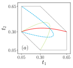
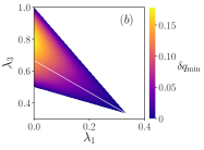
Figure 7: (Color online) (a) Set of points $(t_{1},{t_{2}})$ which can be reached by $SO(3)$ transformations on $\varrho$, for different eigenvector matrices $U$. Permutation $(1,3)$ (solid line), permutation $(1,2)$ (dashed line), and permutation $(2,3)$ (dotted line). (b) The largest difference $\delta q_{\rm min}=q_{\rm wc}-q_{\rm min}$, as a function of the eigenvalues of $\varrho$.

V.2.3 Permutation $(2,3)$

Following the same steps as before, we find expressions for $t_{1}$, $t_{2}$ and $q^{(2,3)}_{\rm min}$. Explicitly, we obtain

$$q^{(2,3)}_{\rm min} =-\,\frac{(1-\lambda_{3}-2\lambda_{1})^{4}}{4\,(1-3\lambda_{3})^{2}}+\frac{(1-\lambda_{3})(1+3\lambda_{3})}{4}\;,$$ (55)

and the resulting curve in $(t_{1},t_{2})$-space can be seen in Fig. 7 (a) as a dotted line.

As mentioned before, we conjecture that all other choices of eigenvector matrices $U$ lead to smaller values for the minimal overlaps over the Wigner $D$-matrices, i.e.,

$$Q(D,\varrho)\leq\max\left(\,q_{\rm min}^{(1,2)}\,,\,q_{\rm min}^{(2,3)}\right)\;,$$ (56)

which is supported by the numerical test given in Fig. 6. Therefore, provided the conjecture holds, we may write

$$q_{\rm wc}=\max\left(q^{(1,2)}_{\rm min}\,,\,q^{(2,3)}_{\rm min}\right)\;.$$ (57)

For $\lambda_{1}=0.05$ and $\lambda_{2}=0.3$, $q_{\rm w}=0.267$, which is taken as the upper tick-mark for the horizontal axis in Fig. 6.

In Fig. 7(b), we plot $\delta q_{\rm min}=q_{\rm wc}-q_{\rm min}$ as a function of the eigenvalues $\lambda_{1}$ and $\lambda_{3}$, where the value of $\delta q_{\rm min}$ is color coded as indicated in the legend of the figure. The white line from $(0,2/3)\quad\mbox{to}\quad(1/3,1/3)$ marks the border between the regiones where $q_{\rm wc}=q^{(1,2)}_{\rm min}$ (above) and $q_{\rm wc}=q^{(2,3)}_{\rm min}$ (below).

VI Conclusions

In this paper we considered the distribution of overlaps between a mixed state and its image under random unitary transformations. For general unitary transformations from $SU(N)$ we showed that the overlap distribution can be computed, in principle, following a method introduced in Ref. Alonso and Gorin (2016). The solution is based on the calculation of the joint probability distribution (JPD) of partial overlaps, for which we could obtain a surprisingly simple analytical expression in the qutrit, i.e., $SU(3)$, case. Based on this result, we obtained a closed expression for the distribution of overlaps, and we solved the inverse problem of estimating the eigenvalues from the overlap distribution and computed the corresponding error estimates.

In the second part of the paper, we assumed that the random transformations are restricted to the subgroup $SO(3)$, in the form of Wigner $D$-matrices. Then, the overlap distribution also depends on the eigenvectors. Choosing some random examples, we find JPD’s for the partial overlaps, with many particular features, which are reflected in the full overlap distribution, also. These may serve as fingerprints for particular mixed quantum states, allowing to verify their identity.

We then focused on the finite range of the overlap distribution, and showed that the $SO(3)$ limits often come quite close to the absolute $SU(3)$ limits, which means that while not exact, eigenvalue estimates based on transformations limited to $SO(3)$ may be useful, provided the error is sufficiently small. Finally, we conjecture that Eq. (57) gives the largest possible difference between the minimal overlap calculated from $SO(3)$ and that calculated from $SU(3)$.

Appendix A Limiting cases for a qutrit ($N=3$)

According to the general expression for the overlap function, Eq. (4), we obtain for the qutrit case

$$Q(O,\varrho) =\lambda_{3}-(\lambda_{3}-\lambda_{1})\;t_{1}-(\lambda_{3}-\lambda_{2})\;t_{2}\;,$$ (58)

where $t_{1}$ and $t_{2}$ are given by Eq. (3). Even without the general solution, we can still solve the following limiting cases. Eventually, we will need the distribution function $\mathcal{P}_{NK}(t)$ of the sum of absolute-value squares of $K$ elements of column vectors of $O$ in $N=3$ dimensions. These functions have been calculated in Ref. Alonso and Gorin (2016).

A.1 $\lambda_{1}=\lambda_{2}=\lambda_{3}=1/3$

For this case we simply have

$$Q(O,\varrho)=\frac{1}{3},\quad P_{\varrho}(q)=\langle\delta(q-1/3)\rangle\;.$$ (59)

A.2 $\lambda_{1}=0,\lambda_{2}=\lambda_{3}=1/2$

For this case we have,

$$Q(O,\varrho) =\frac{1}{2}(1-t_{1})\;,$$

$$\mbox{with}\quad t_{1} =\frac{|O_{21}|^{2}+|O_{31}|^{2}}{2}=\frac{1-|O_{11}|^{2}}{2}\;,$$ (60)

since the matrix $O$ is unitary. Therefore,

$$Q(O,\varrho) =\frac{1+|O_{11}|^{2}}{4}\;.$$ (61)

With this result, the probability density becomes

$$P_{\varrho}(q) =\langle\;\delta\left(q-Q(O,\varrho)\right)\;\rangle=\left\langle\delta\left(q-\frac{1+|O_{11}|^{2}}{4}\right)\;\right\rangle$$

$$=\int_{0}^{1}{\rm{d}}t\;\mathcal{P}_{31}(t)\;\delta\left(q-\frac{1+t}{4}\right)$$

$$=4\int_{1/4}^{1/2}{\rm{d}}q^{\prime}\;\mathcal{P}_{31}(4q^{\prime}-1)\;\delta\left(q-q^{\prime}\right)\;,$$ (62)

and finally

$$P_{\varrho}(q)=4\mathcal{P}_{31}(4q-1)\quad\text{for}\quad 1/4\leq q\leq 1/2$$ (63)

and zero otherwise.

A.3 $\lambda_{1}=\lambda_{2}=0,\lambda_{3}=1$

We have

$$Q(O,\varrho) =1-t_{1}-t_{2},$$

$$=1-\left(|O_{31}|^{2}+|O_{32}|^{2}\right)=|O_{33}|^{2},$$ (64)

with $t_{1}=|O_{31}|^{2}$, $t_{2}=|O_{32}|^{2}$, and $|O_{31}|^{2}+|O_{32}|^{2}+|O_{33}|^{2}=1$. Hence,

$$Q(O,\varrho)=|O_{33}|^{2},\quad P_{\varrho}(q)=\mathcal{P}_{31}(q)\;.$$ (65)

Appendix B Details of the JPD calculation for $N=3$

Here, we will provide some details on the evaluation of the integrals, which finally lead to Eq. (26) for the JPD of the partial overlaps in the qutrit case. The starting point is the following integral

$$\int\frac{\text{d}s_{1}}{2\pi}\;\frac{1}{\prod_{j=1}^{3}\det[\bm{C}(\lambda_{j})]}.$$ (66)

The general method is shown here for the two orderings that give non-trivial results using formulas in Appendix C when needed.

B.1 Case a) $\quad 0<\lambda_{1}<t_{1}<\lambda_{2}<\lambda_{3}$

Here the three poles are given by

$$z_{j}=\frac{i}{t_{1}-\lambda_{j}}\left[1+\frac{|\tau|^{2}}{4\,c_{2}(\lambda_{j})}\,\right],\quad j=1,2,3,$$ (67)

such that $z_{1}$ lies on the upper half plane, while $z_{2}$ and $z_{3}$ are lying on the lower one. Thus, we close the integration over the upper half plane, which results in a positively oriented closed curve around the pole at $z_{1}$.

Using the formula form Appendix C.1, the integral over $s_{1}$ can be written as

$$\int\frac{\text{d}s_{1}}{2\pi}\;\frac{1}{\prod_{j=1}^{3}\det[\bm{C}(\lambda_{j})]}=\frac{-(\lambda_{1}-t_{1})c_{2}(\lambda_{1})}{(a_{12}+b_{12}|\tau|^{2})(a_{13}+b_{13}|\tau|^{2})},$$ (68)

where we have defined

$$a_{jk} \equiv(\lambda_{j}-\lambda_{k})c_{2}(\lambda_{j})c_{2}(\lambda_{k}),$$ (69)

$$b_{jk} \equiv\frac{1}{4}[(\lambda_{j}-t_{1})c_{2}(\lambda_{j})-(\lambda_{k}-t_{1})c_{2}(\lambda_{k})].$$ (70)

Next, we perform the integral over $\tau$ on the result using the formula in Appendix C.2,

$$-(\lambda_{1}-t_{1}) c_{2}(\lambda_{1})\int\frac{\text{d}\tau^{2}}{4\pi^{2}}\frac{1}{(a_{12}+b_{12}|\tau|^{2})(a_{13}+b_{13}|\tau|^{2})}$$

$$=\frac{-(\lambda_{1}-t_{1})c_{2}(\lambda_{1})}{4\pi}\frac{\ln(a_{12}b_{13})-\ln(a_{13}b_{12})}{a_{12}b_{13}-a_{13}b_{12}}.$$ (71)

Now, we want to perform the final integral in $s_{2}$, the dependence on this variable is hidden in $a_{jk}$ and $b_{jk}$ through $c_{2}(\lambda_{k})$. Let us make this dependence explicit by the replacements

$$a_{12}b_{13}-a_{13}b_{12}= \frac{1}{4}(t_{1}-\lambda_{1})(\lambda_{1}-\lambda_{2})(\lambda_{1}-\lambda_{3})$$

$$\times(\lambda_{2}-\lambda_{3})s_{2}^{2}[1+is_{2}(t_{2}-\lambda_{1})],$$ (72)

where

$$\frac{a_{12}b_{13}}{a_{13}b_{12}}=\frac{1+is_{2}(t_{2}-\lambda_{2})}{1+is_{2}(t_{2}-\lambda_{3})}\cdot\frac{1+is_{2}(t_{1}-\lambda_{1}+t_{2}-\lambda_{3})}{1+is_{2}(t_{1}-\lambda_{1}+t_{2}-\lambda_{2})},$$ (73)

simplifying, we obtain

$$\int\frac{\text{d}s_{2}}{2\pi}\dots=\frac{1}{2\pi^{2}(\lambda_{1}-\lambda_{2})(\lambda_{1}-\lambda_{3})(\lambda_{2}-\lambda_{3})}$$

$$\times\int\frac{\text{d}s_{2}}{s_{2}^{2}}\ln\left[\frac{1+is_{2}(t_{2}-\lambda_{2})}{1+is_{2}(t_{2}-\lambda_{3})}\cdot\frac{1+is_{2}(t_{1}-\lambda_{1}+t_{2}-\lambda_{3})}{1+is_{2}(t_{1}-\lambda_{1}+t_{2}-\lambda_{2})}\right].$$ (74)

The integral is performed in Appendix C.3 and the result is

$$\int\frac{\text{d}s_{2}}{2\pi} \dots=\frac{|t_{2}-\lambda_{2}|-|t_{2}-\lambda_{3}|}{2\pi(\lambda_{1}-\lambda_{2})(\lambda_{1}-\lambda_{3})(\lambda_{2}-\lambda_{3})}$$

$$+\frac{|t_{1}+t_{2}-\lambda_{1}-\lambda_{3}|-|t_{1}+t_{2}-\lambda_{1}-\lambda_{2}|}{2\pi(\lambda_{1}-\lambda_{2})(\lambda_{1}-\lambda_{3})(\lambda_{2}-\lambda_{3})}.$$ (75)

Then, in order to obtain $\mathcal{P}_{\lambda}(t_{1},t_{2})$ we must calculate $Z(\bm{0})$, given by $Z(\bm{s})$ in Eq. (15) with $s_{j}=0$. It is then given by the following integral that can be solved straightforward

$$Z(\bm{0})=\int\frac{\text{d}\tau^{2}}{4\pi^{2}}\frac{1}{\left(1+\frac{|\tau|^{2}}{4}\right)^{3}}=\frac{1}{2\pi}.$$ (76)

Thus, finally for ordering (a)

$$\mathcal{P}_{\lambda}(t_{1},t_{2}) =\frac{|t_{1}+t_{2}-\lambda_{1}-\lambda_{3}|-|t_{1}+t_{2}-\lambda_{1}-\lambda_{2}|}{(\lambda_{1}-\lambda_{2})(\lambda_{1}-\lambda_{3})(\lambda_{2}-\lambda_{3})}$$

$$+\frac{|t_{2}-\lambda_{2}|-|t_{2}-\lambda_{3}|}{(\lambda_{1}-\lambda_{2})(\lambda_{1}-\lambda_{3})(\lambda_{2}-\lambda_{3})}.$$ (77)

B.2 Case b) $\quad 0<\lambda_{1}<\lambda_{2}<t_{1}<\lambda_{3}$

Here, there are two poles in the upper half plane given by $z_{1}$ and $z_{2}$. We can calculate the first integral on $s_{1}$ with the residue theorem again but now with two poles, i.e.,

$$\int\frac{\text{d}s_{1}}{2\pi}\;\frac{1}{\prod_{j=1}^{3}\det[\bm{C}(\lambda_{j})]}$$

$$=\left.\frac{i}{\det\bm{C}(\lambda_{2})\det\bm{C}(\lambda_{3})}\right|_{s_{1}=z_{1}}\;{\rm Res}\left(\frac{1}{\det[\bm{C}(\lambda_{1})]},z_{1}\right)$$

$$+\left.\frac{i}{\det\bm{C}(\lambda_{1})\det\bm{C}(\lambda_{3})}\right|_{s_{1}=z_{2}}\;{\rm Res}\left(\frac{1}{\det[\bm{C}(\lambda_{2})]},z_{2}\right).$$ (78)

The first integral is exactly the one we calculated in case (a). The second integral has a similar form and we can use the same integration method. The second residue is

$${\rm Res}\left(\frac{1}{\det[\bm{C}(\lambda_{2})]},z_{2}\right)=\frac{i}{(\lambda_{2}-t_{1})c_{2}(\lambda_{2})},$$ (79)

and using the formula from Appendix C.1, we can calculate $\left.\det\bm{C}(\lambda_{k})\right|_{s_{1}=z_{2}}$ for $k=1,3$. With these equations, we can obtain that the new part of the integral in $s_{1}$, given by the residue in $z_{2}$ is

$$\left.\frac{i}{\det\bm{C}(\lambda_{1})\det\bm{C}(\lambda_{3})}\right|_{s_{1}=z_{2}}{\rm Res}\left(\frac{1}{\det[\bm{C}(\lambda_{2})]},z_{2}\right)$$

$$\qquad\qquad=\frac{-(\lambda_{2}-t_{1})c_{2}(\lambda_{2})}{(a_{21}+b_{21}|\tau|^{2})(a_{23}+b_{23}|\tau|^{2})}.$$ (80)

The integral over $\tau$ is solved using the formula from Appendix C.2 as

$$-(\lambda_{2}-t_{1}) c_{2}(\lambda_{2})\int\frac{\text{d}\tau^{2}}{4\pi^{2}}\frac{1}{(a_{21}+b_{21}|\tau|^{2})(a_{23}+b_{23}|\tau|^{2})}$$

$$=\frac{-(\lambda_{2}-t_{1})c_{2}(\lambda_{2})}{4\pi}\frac{\ln(a_{21}b_{23})-\ln(a_{23}b_{21})}{a_{21}b_{23}-a_{23}b_{21}}.$$ (81)

Replacing the definitions of $a_{jk}$ and $b_{jk}$ for $c_{2}(\lambda_{j})$ and $c_{2}(\lambda_{k})$ and then to $s_{2}$, we obtain

$$a_{21}b_{23}-a_{23}b_{21}=\frac{1}{4}(t_{1}-\lambda_{2})(\lambda_{2}-\lambda_{1})(\lambda_{2}-\lambda_{1})(\lambda_{1}-\lambda_{3})$$

$$\hskip 76.82243pt\times s_{2}^{2}[1+is_{2}(t_{2}-\lambda_{2})],$$ (82)

$$\frac{a_{21}b_{23}}{a_{23}b_{21}}=\frac{1+is_{2}(t_{2}-\lambda_{1})}{1+is_{2}(t_{2}-\lambda_{3})}\cdot\frac{1+is_{2}(t_{1}-\lambda_{2}+t_{2}-\lambda_{3})}{1+is_{2}(t_{1}-\lambda_{2}+t_{2}-\lambda_{1})},$$ (83)

simplifying, we obtain

$$\int\frac{\text{d}s_{2}}{2\pi}\dots=\frac{1}{2\pi^{2}(\lambda_{2}-\lambda_{3})(\lambda_{2}-\lambda_{1})(\lambda_{1}-\lambda_{3})}$$

$$\times\int\frac{\text{d}s_{2}}{s_{2}^{2}}\ln\left[\frac{1+is_{2}(t_{2}-\lambda_{1})}{1+is_{2}(t_{2}-\lambda_{3})}\cdot\frac{1+is_{2}(t_{1}-\lambda_{2}+t_{2}-\lambda_{3})}{1+is_{2}(t_{1}-\lambda_{2}+t_{2}-\lambda_{1})}\right].$$ (84)

This integral in $s_{2}$ is given by the formula in Appendix C.3, therefore

$$\int \frac{\text{d}s_{2}}{2\pi}\dots=\frac{|t_{2}-\lambda_{1}|-|t_{2}-\lambda_{3}|}{2\pi(\lambda_{2}-\lambda_{3})(\lambda_{2}-\lambda_{1})(\lambda_{1}-\lambda_{3})}$$

$$+\frac{|t_{1}+t_{2}-\lambda_{2}-\lambda_{3}|-|t_{1}+t_{2}-\lambda_{1}-\lambda_{2}|}{2\pi(\lambda_{2}-\lambda_{3})(\lambda_{2}-\lambda_{1})(\lambda_{1}-\lambda_{3})}.$$ (85)

Using the calculated value of $Z(\bm{0})=(2\pi)^{-1}$ and the value of the integral of part (a), we obtain

$$\mathcal{P}_{\lambda}(t_{1},t_{2})= \frac{|t_{1}+t_{2}-\lambda_{1}-\lambda_{3}|-|t_{1}+t_{2}-\lambda_{2}-\lambda_{3}|}{(\lambda_{1}-\lambda_{2})(\lambda_{1}-\lambda_{3})(\lambda_{2}-\lambda_{3})}$$

$$+\frac{|t_{2}-\lambda_{2}|-|t_{2}-\lambda_{1}|}{(\lambda_{1}-\lambda_{2})(\lambda_{1}-\lambda_{3})(\lambda_{2}-\lambda_{3})}.$$ (86)

Appendix C Integration formulas

C.1 Integrals over $s_{1}$

The following integral

$$\int\frac{\text{d}s_{1}}{2\pi}\frac{1}{\prod_{j=1}^{3}\det[\bm{C}(\lambda_{j})]} =\left.\frac{i}{\det\bm{C}(\lambda_{2})\det\bm{C}(\lambda_{3})}\right|_{s_{1}=z_{1}}$$

$$\times{\rm Res}\left(\frac{1}{\det[\bm{C}(\lambda_{1})]},z_{1}\right),$$ (87)

where the residue is given by

$${\rm Res}\Big{(}\frac{1}{\det[\bm{C}(\lambda_{j})]},z_{j}\Big{)}=\frac{i}{(\lambda_{j}-t_{1})\,c_{2}(\lambda_{j})},$$ (88)

in this case with $j=1$. The evaluation of $\det\bm{C}(\lambda_{k})$ at $s_{1}=z_{j}$ is given by

$$\left.\det\bm{C}(\lambda_{j})\right|_{s_{1}=z_{j}}=a^{\prime}_{jk}+b^{\prime}_{jk}|\tau|^{2},$$ (89)

with

$$a^{\prime}_{jk} \equiv\frac{\lambda_{j}-\lambda_{k}}{\lambda_{j}-t_{1}}c_{2}(\lambda_{k}),$$ (90)

$$b^{\prime}_{jk} \equiv\frac{1}{4}\left(1-\frac{\lambda_{k}-t_{1}}{\lambda_{j}-t_{1}}\frac{c_{2}(\lambda_{k})}{c_{2}(\lambda_{j})}\right).$$ (91)

After simplifying, the integral over $s_{1}$ can be written as

$$\int\frac{\text{d}s_{1}}{2\pi}\;\frac{1}{\prod_{j=1}^{3}\det[\bm{C}(\lambda_{j})]}=\frac{-(\lambda_{1}-t_{1})c_{2}(\lambda_{1})}{(a_{12}+b_{12}|\tau|^{2})(a_{13}+b_{13}|\tau|^{2})},$$ (92)

where we have defined

$$a_{jk} \equiv(\lambda_{j}-\lambda_{k})c_{2}(\lambda_{j})c_{2}(\lambda_{k}),$$ (93)

$$b_{jk} \equiv\frac{1}{4}[(\lambda_{j}-t_{1})c_{2}(\lambda_{j})-(\lambda_{k}-t_{1})c_{2}(\lambda_{k})].$$ (94)

C.2 $\tau$-integral

This integral is

$$\int\frac{\text{d}\tau^{2}}{4\pi^{2}}\frac{1}{(a_{1}+b_{1}|\tau|^{2})(a_{2}+b_{2}|\tau|^{2})}$$ (95)

We write $\tau$ in polar coordinates as $\tau=r\text{e}^{i\theta}$ to integrate

$$\int_{0}^{2\pi} \frac{\text{d}\theta}{4\pi^{2}}\int_{0}^{\infty}\frac{r\text{d}r}{(a_{1}+b_{1}r^{2})(a_{2}+b_{2}r^{2})}$$

$$=\frac{1}{2\pi}\left.\frac{\ln(a_{1}+b_{1}r^{2})-\ln(a_{2}+b_{2}r^{2})}{2(a_{2}b_{1}-a_{1}b_{2})}\right|_{0}^{\infty}$$

$$=\frac{1}{4\pi}\frac{\ln(a_{1}b_{2})-\ln(a_{2}b_{1})}{a_{1}b_{2}-a_{2}b_{1}}.$$ (96)

C.3 Integrals over $s_{2}$

The $s_{2}$ integral is given by

$$\int_{-\infty}^{\infty}\frac{\text{d}x}{x^{2}} \ln\left[\frac{1+iq_{1}x}{1+iq_{2}x}\cdot\frac{1+iq_{3}x}{1+iq_{4}x}\right]$$

$$= \;\pi\left(|q_{1}|-|q_{2}|+|q_{3}|-|q_{4}|\right).$$ (97)

References

- Paris and Rehacek (2004) M. Paris and J. Rehacek, eds., Quantum state estimation (Springer, Lecture notes in physics, 2004).
- Häffner et al. (2005) H. Häffner, W. Hänsel, C. F. Roos, J. Benhelm, D. C. al kar, M. Chwalla, T. Körber, U. D. Rapol, M. Riebe, P. O. Schmidt, C. Becher, O. Gühne, W. Dür, and R. Blatt, Nature 438, 643 (2005).
- Cramer et al. (2010) M. Cramer, M. B. Plenio, S. T. Flammia, R. Somma, D. Gross, S. D. Bartlett, O. Landon-Cardinal, D. Poulin, and Y.-K. Liu, Nature Communications 1, 149 (2010).
- Keyl and Werner (2001) M. Keyl and R. F. Werner, Phys. Rev. A 64, 052311 (2001).
- Ballester (2006) M. A. Ballester, Journal of Physics A: Mathematical and General 39, 1645 (2006).
- Tanaka et al. (2014) T. Tanaka, Y. Ota, M. Kanazawa, G. Kimura, H. Nakazato, and F. Nori, Phys. Rev. A 89, 012117 (2014).
- van Enk and Beenakker (2012) S. J. van Enk and C. W. J. Beenakker, Phys. Rev. Lett. 108, 110503 (2012).
- Walborn et al. (2006) S. P. Walborn, P. H. Souto Ribeiro, L. Davidovich, F. Mintert, and A. Buchleitner, Nature 440, 1022 (2006).
- Walborn et al. (2007) S. P. Walborn, P. H. S. Ribeiro, L. Davidovich, F. Mintert, and A. Buchleitner, Phys. Rev. A 75, 032338 (2007).
- Filip (2002) R. Filip, Phys. Rev. A 65, 062320 (2002).
- Bartkiewicz et al. (2013) K. Bartkiewicz, K. Lemr, and A. Miranowicz, Phys. Rev. A 88, 052104 (2013).
- Bianchetti et al. (2010) R. Bianchetti, S. Filipp, M. Baur, J. M. Fink, C. Lang, L. Steffen, M. Boissonneault, A. Blais, and A. Wallraff, Phys. Rev. Lett. 105, 223601 (2010).
- Vitanov (2012) N. V. Vitanov, Phys. Rev. A 85, 032331 (2012).
- Alonso and Gorin (2016) L. Alonso and T. Gorin, Journal of Physics A: Mathematical and Theoretical 49, 145004 (2016).
- Sakurai (1994) J. J. Sakurai, Modern Quantum Mechanics, revised edition ed. (Addison Wesley, Reading, Massachusetts, 1994).
- Haar (1933) A. Haar, Ann. Math. 34, 147 (1933).
- Weyl (1939) H. Weyl, The classical groups (Princton University Press, Princton, 1939).
- Znidaric and Prosen (2003) M. Znidaric and T. Prosen, Journal of Physics A: Mathematical and General 36, 2463 (2003), marko Žnidarič and Tomaž Prosen.
- Gorin et al. (2006) T. Gorin, T. Prosen, T. H. Seligman, and M. Žnidarič, Phys. Rep. 435, 33 (2006).
- Nielsen and Chuang (2000) M. A. Nielsen and I. L. Chuang, quantum computation and quantum information (Cambridge University Press, Cambridge, 2000).
- Note (1) The shape of may be varying between vector and diagonal matrix form, depending on the context.
- Burlakov et al. (2003) A. V. Burlakov, L. A. Krivitskii, S. P. Kulik, G. A. Maslennikov, and M. V. Chekhova, Optics and Spectroscopy 94, 684 (2003).